DEPARTMENT OF ECONOMICSWORKING PAPERS

economics.ceu.hu

AS-AD in the Standard Dynamic NeoclassicalModel: Business Cycles and Growth Trends

by

Max Gillman1

2012/8

1 Department of Economics, Central European University, Cardiff Business School, Cardiff, UK, gillmanm@cf.ac.uk

Abstract

The paper shows how a dynamic neoclassical AS-AD can be derived and used to describe business cycles and

growth trends to undergraduates. Derived within the Ramsey-Cass-Koopmans (RCK) model, the AS-AD is the

stationary equilibrium of the deterministic dynamic general equilibrium framework. Allowing Solow exogenous

growth, the AS-AD is derived along the balanced growth path equilibrium. The derivation first builds

consumption demand, aggregate demand, and then aggregate supply through the equilibrium conditions and a

closed form solution for the capital stock. Through a comparative static change in goods sector productivity, the

paper shows the basic failing of the standard RBC model. Allowing a second comparative static change in the

consumer's time endowment, this captures a change in the "external margin" of labor supply. These comparative

statics enable explanation of the business cycle, and "Solow-plus" growth trends including education time and

working time. In extension of RCK, the paper shows beyond the undergraduate level, how to derive AS-AD when

including human capital and endogenous growth. This allows an endogenous change in the time endowment for

work and leisure through a change in human capital productivity, with a similar but more fundamental AS-AD

story of business cycles and growth trends.

Key words: Ramsey-Cass-Koopmans, supply, demand, state variables

JEL Numbers: A22, A23, E13

Acknowledgements

I thank Vito Polito for comments.

1 Introduction

Colander (1995) famously clari�es how the aggregate supply and aggregatedemand (AS�AD) analysis is derived in part from the Keynesian model andis "incorrectly speci�ed". It lacks internal consistency in that it combines aKeynesian demand which implicitly assumes an unknown supply condition,and then adds a classical supply curve, thereby mixing analyses. At the heartof the Keynesian demand is the Keynesian "cross" that goes back at leastto Samuelson�s (1951) seminal formulation. Samuelson starts with a "�tted"consumption expenditure schedule with a slope less than one graphed arounda 45 degree line (p. 266). This becomes the basis of the standard derivationof the Keynesian demand. In contrast, Friedman (1957) puts forth that theKeynesian assumption about the nature of the consumption function is notonly important but also wrong, a debate that ensues today. Friedman o¤ersthe alternative of instead deriving a "classical" consumption demand that isa fraction of permanent income, using Fisher�s intertemporal analysis.Colander (1995) suggests making the Keynesian AD consistent with a

Keynesian AS; perhaps through a focus on how the price level is determined.Originally, Fisher derived the price level as a function of the money supplyin his quantity theory. Keynes (1923) embraced this Fisher derivation in hisTract, but Keynes (1930) radically departs from its price level determinationin his Treastise. Instead Keynes follows his teach Marshall and writes theaggregate price as the aggregate average cost plus aggregate pro�t. HoweverKeynes (1930) assumes that pro�t equals investment minus savings, whichhe defends in footnotes to his 1936 GeneralTheory, but which has no basisin Marshallian theory.1

This paper could be said to formulate AS � AD by following in partboth Keynes�s (1930) fascinating Marshall-based attempt and Friedman�sFisher-based consumption theory. It derives consumption demand as in the

1Gillman (2002) argues that the Keynesian cross analysis is based on the incorrectassumption that pro�t equals investment (I) minus savings (S), as in Keynes�s (1930)Treatise on Money. The Treatise presents a "cross" and business cycle whereby I exceedingS causes pro�t that leads to expansion, while I<S leads to contraction, with a "stable"equilibrium at I=S where the cross intersection occurs. In modern micro-founded realbusiness cycle theory, the representative agent �nds I=S in equilibrium, pro�t is de�nedresidually as revenue minus cost, and such a dynamic basis for a business cycle through Iand S is not explicitly postulated.

2

permanent income hypothesis of consumption, but as an outcome of utilityoptimization rather that as any sort of assumption. Aggregate demand thenadds the consumption demand to investment, while aggregate supply is the�rm�s normalized upward sloping marginal cost curve. The elusive aggregateprice of the AS�AD analysis is simply a relative price as in all micro theory,in this case of goods to leisure (or labor if one prefers). Its "balanced growthpath" (BGP ) time-less solution bypasses the time dimension that Colandernotes exists in the context of classic AS supply curves that are describedas short, medium or long run. Instead the AS � AD presented here is the"stationary equilibrium" that we (in misnomer?) often call the long run. Aswas the aim of Keynes (1930), the (relative) price of output is not tied up inany way with monetary theory, the quantity theory of money in particular,or with any money stock at all. Rather the price is simply the inverse of thereal wage rate given that the goods price is normalized to one. In turn, in thelabor market the relative price is the real wage rate divided by one. Monetarytheory can be added within an AS � AD extension (Gillman, 2011), but isbeyond the scope of this initial presentation of the "neoclassical" AS �AD:The precise AS � AD presented is simply that of the Ramsey (1928)-

Cass (1965)-Koopmans (1965) [RCK] model. And while Colander (1995)rightly focuses on the intricacies of the dynamics involved in telling the AS�AD stories of Keynesian origin, also discussed in Gillman (2002), here themodel is fuly dynamic but only the BGP equilibrium is presented. Transitiondynamics are not investigated. Comparative statics show the new BGP

equilibrium when an exogenous parameter is changed. Only two comparativestatic changes are presented here. They provide analysis of the central focusof modern macroeconomics: the business cycle and growth theory. Andwhile rigorous, only partial derivatives and algebraically solving systems ofequations is required. The RCK derived AS � AD is an equilibrium of adynamic model and so naturally has complexity. But arguably it is withinreach of advanced undergraduates and, in my pure speculation, is the futurefor undergraduate teaching as mathematical description become increasinglyaccepted over time as in any science.Surprisingly it appears that never before has AS �AD been derived rig-

orously within our standard dynamic general equilibrium framework. Suchderivation is the paper�s main contribution. Making it accessible to under-

3

graduates is a second contribution. And its other contribution is to use onlytwo comparative static changes to explain qualitative business cycles andgrowth trends. It does this with no assumptions beyond standard parame-ter calibration for utility and production within the standard RCK modelof neoclassical exogenous growth. Allowing for positive Solow exogenoustechnological progress, AS � AD is shown to be equally well-derived withsustained growth. Extension to endogenous growth follows rather seamlesslyand improves key aspects of the "macroeconomic story we tell"; as this getsbeyond undergraduate reach, but helps motivate the comparative statics usedin the RCK model, this extension is brie�y sketched as well.Motivation for the paper is clear. It bridges a daunting a gap for students

of microeconomics embarking upon the study of macroeconomics. In modernmacroeconomic teaching, microeconomic derived supply and demand analysiswith comparative statics is left behind. In advanced macro research, it isreplaced by numerical simulation of the equilibrium with impulse responses toshocks. The advantage of graphical market analysis has been lost even thoughit lurks just below the surface of our foundation modern macro researchmodels. The paper�sAS�AD �lls the micro to macro void that has befuddledus since the dawn of modern macro general equilibrium theory.

2 Modeling Overview

Widespread adoption of the recursive methodology, stimulated for exampleby Stokey, Lucas and Prescott (1989), seemingly has pushed AS �AD evenfarther from the underlying markets based on supply and demand. Ironicallyit is the recursive methodology itself that holds a key to a "restart" of teachingmodern macro with the supply and demand of micro. This key is the so-called state variable. This is the stock variable of the system which hasits accumulation stated in discrete time as a �rst-order di¤erence equation.And for typical timing conventions, the current period stock is known inthe current time period while the choice of the stock for next period is thedecision variable. The RCK known state variable at time t is the capitalstock at time t; denoted here by kt. The �rst trick to forming AS � AD isto exploit exactly this fact that the equilibrium kt is known at time t:The second trick is to identify AS � AD as we would in micro: at the

4

"stationary" equilibrium. In the dynamic world of RCK with capital accu-mulation and Solow (1956) growth, this equilibrium is the BGP equilibriumwith either zero or some positive rate of exogenous growth. The formulationof AS � AD makes supply and demand a function of kt: This is similar tohow partial equilibrium demand typically is a function of exogenously givenincome, except that kt is an endogenously determined equilibrium value. Thecapital stock can solved as a closed-form solution of exogenous parameters byusing market clearing to set AS equal to AD at the equilibrium relative price(or the real wage); it then in addition requires using the exogenous growthaspect of RCK to solve uniquely for the real wage in terms of exogenousparameters. This leaves the goods market clearing condition as one equationin kt; with an explicit kt solution..Deriving AS�AD in the RCK model, as a function of kt; involves using

the RCK equilibrium conditions to solve the same two margins we alreadyteach and derive in textbook-style to varying degrees: the intratemporal mar-ginal rate of substitution between goods and leisure and the intertemporalmargin between consumption this period and next period. From these mar-gins, the permanent income hypothesis of consumption demand is formed.Construction of the AS � AD follows readily, along with the supply anddemand for labor, also contigent on kt:A change in any exogenous parameter implies a new kt in the BGP equi-

librium, and a new set of AS�AD curves. In addition to changing the capitalstock, an exogenous parameter change directly cause shifts in the supply anddemand functions. So parameter changes cause changes in the equilibriumkt, which shifts the AS � AD, and also the parameters directly enter theAS � AD functions and cause additional shifts.The main comparative static exercise of neoclassical growth and real busi-

ness cycles (RBC) is a change in the goods sector productivity parameter.Doing this within the AS �AD framework can illustrate the stark but well-known result that shows the central failure of the standard RBC model toexplain business cycles. Using the homothetic utility and production func-tions, employment does not change when goods sector productivity changes,in contrast to actual business cycle experience. This gives a deterministicrendering of RBC theory whereby the income and substitution e¤ects of thewage rate change o¤set each other and leave employment unchanged. Using

5

log-utility and Cobb-Douglas production throughout the paper, this compar-ative static also illustrates an equally well-known result in growth theory. Atrend up in productivity over time results in hours worked staying constantrather than trending downwards as in data. The downward trend has beenexplained in a variety of ways. Call this a "Solow-plus" trend that we wouldprefer to capture if we could while still explaining the other Solow growthfacts.2

Illustrating for the student central failings of the RCK model clears theway to embark upon a neat solution. To see a way to breathe new life into theRCK model, consider what a change in the goods sector productivity (TFP)actually does. Given the production technology, an increase in TFP raises theconsumer�s endowment of goods. Our neoclassical growth and business cycleanalysis rests on this one side of our endowed world. The other dimension ofthe consumer endowment, Beckerian (1965) time, is ignored.The solution is to allow not just the goods endowment to change, but

rather both goods and time endowments to change. Allowing both endow-ments exogenously to rise and fall in comparative static fashion shows abusiness cycle in the AS�AD of the goods market and in the labor market.Allowing for certain exogenous trends in both goods and time endowmentgives the standard Solow facts plus the trend down in hours worked per week.Fortunately, the additional change in the time endowment not only bal-

ances out our treatment of considering changes in total endowment, goodsand time, but is also consistent with how research has extended the stan-dard model to better explain both business cycles and growth. Exogenouslychanging the time endowment given for work and leisure within the RCKmodel is similar to changing the "external" labor margin, which is sometimesthought of as the "labor force participation rate". Adding an external la-bor margin has been found to be a key to explaining cycles with an RBCapproach.3 In extension to endogenous growth, the time left for work andleisure becomes endogenous when there is a second sector using time to pro-duce human capital investment. A change in the productivity of the human

2These four Solow facts are a constant real interest rate and output to capital ratio,and a rising real wage and output to labor ratio.

3See Hansen (1985) and Rogerson (1988), along with the closely related two sectorextensions of Benhabib et al (1991) and Greenwood and Hercowitz (1991).

6

capital sector, in general, causes a change in the time allocated for work andleisure.4

3 Analysis

Let the representative agent act as both �rm and consumer. The �rm rentscapital kt from the consumer at the real competitive rate rt and pays wagesfor labor time lt at the competitive rate wt: The �rm�s production technologyfor goods output yt is Cobb-Douglas with AG � 0 and 2 [0; 1] :

yt = AG (lt) (kt)

1� :

The �rm pro�t �t maximization yields that the wage rate and capital rentalrate equal their respective marginal products:

Maxlt;kt

�t = AG (lt) (kt)

1� � wtlt � rtkt;

wt = AG (lt) �1 (kt)

1� ;

rt = (1� )AG (lt) (kt)� :

The consumer�s period t utility is of log form in goods ct and in leisurext; such that with the leisure preference parameter � � 0;

u (ct; xt) = ln ct + � lnxt:

The consumer spends time working for the �rm, lt; and time in leisure, suchthat the total time endowment is equal to T :

T = lt + xt:

The consumer�s goods budget constraint sets expenditure on consumption ctequal to income from wages wtlt and capital rental rtkt minus investment incapital it: With �K 2 [0; 1] the depreciation rate on capital stock, it is givenby

it = kt+1 � kt (1� �K) :4This literature dates to Uzawa�s (1965) two sector model with human capital, which

was modernized by RCK-style utility maximization in Lucas (1988).

7

The goods constraint is then

ct = wtlt + rtkt � kt+1 + kt (1� �K) :

The consumer maximization problem is over the discounted in�nite horizon,with � 2 (0; 1) � 1

1+�being the discount factor, with �t the Lagrangian

multiplier on the goods constraint, with �t the Lagrangian multiplier on thetime constraint, and with the choice being with respect to consumption ofgoods ct; leisure xt; and next period�s capital stock kt+1 :

Maxct;xt;lt;kt+1

1Xt=0

�tfln ct + � lnxt

+�t [wtlt + rtkt � kt+1 + kt (1� �K)� ct]+�t [T � lt � xt]g:

Or eliminating the constraints, the problem is equally stated as

Maxlt;kt+1

1Xt=0

�tfln [wtlt + rtkt � kt+1 + kt (1� �K)] + � ln (T � lt)g:

When taking the �rst-order conditions, the problem requires writing out theconstrained utility in two adjacent time periods: t and t+ 1: This is becausenext period�s capital stock kt+1 appears in the goods resource constraint attime t and at time t + 1: The equilibrium conditions give the consumer�sintratemporal marginal rate of substitution between goods and leisure andthe intertemporal marginal rate of substitution between consumption at timet and at time t+ 1:The nature of the in�nite horizon problem that requires a focus on only

two periods, t and t + 1; immediately lends itself to the simpler recursiveframework that indeed uses only those two periods. In particular, throughin�nite substitution the present discounted value of the in�nitely discountedutility can be written simply over the two periods t and t + 1: Call themaximized Lagrangian V (kt) : Then the problem rewrites in recursive formas

V (kt) = Maxct;xt;lt;kt+1

fln ct + � lnxt + �V (kt+1)

+�t [wtlt + rtkt � kt+1 + kt (1� �K)� ct]+�t [T � lt � xt]g:

8

With constraints substituted in,

V (kt) =Maxlt;kt+1

ln [wtlt + rtkt � kt+1 + kt (1� �K)] +� ln (T � lt) + �V (kt+1) :

In addition to the two �rst-order conditions, equilibrium requires the envelopecondition of the derivative with respect to the state variable kt:

wtct� �

xt= 0;

�1ct+ �

@V (kt+1)

@kt+1= 0;

@V (kt)

@kt=

1 + rt � �kct

:

Eliminating @V (kst )

@kstand

@V (kst+1)@kst+1

and de�ning the rate of time preference � as11+�

� �; the equilibrium conditions reduce to the goods and time constraintsplus the intratemporal and intertemporal margins that are

�xt1ct

= wt;ct+1ct

=1 + rt � �k1 + �

:

3.1 Aggregate Demand: AD

Use the allocation of time constraint to solve for labor supply lst = T � xt:Substitute in for xt = �ct

wtfrom the intratemporal margin so that lst = T� �ct

wt:

Then substitute in for lst in the budget constraint: ct = wt�T � �ct

wt

��kt+1+

kt (1 + rt � �K) : Solving for consumption demand, ct = wtT�kt+1+kt(1+rt��K)1+�

:

Bringing together terms such that ct =wtT+kt

�� kt+1

kt+1+rt��k

�1+�

, the BGP so-lution sees all non-stationary variables growing at the same rate, say g: Thenconsumption demand is

ct =wtT + kt (rt � �k � g)

1 + �

The intertemporal margin along the BGP implies that 1+g = ct+1ct= 1+rt��k

1+�;

so that rt � �k � g = � (1 + g) ; and ct = wtT+kt�(1+g)1+�

:

In the baseline case, set the exogenous growth rate to zero, so that g = 0;r = �+ �k; and ct =

wtT+kt�1+�

: Consumption is a fraction of permanent incomeypt � wtT + �kt:

ct =1

1 + �(wT + �k) � ypt

1 + �:

9

Consumption is a fraction of the �ow of the full value of time plus the in-terest �ow of capital, with the fraction a function of how much leisure ispreferred. This is the permanent income hypothesis of consumption withinthe deterministic RCK model.Adding stationary investment demand means adding the maintenance of

capital or �kk to consumption demand. This give a BGP aggregate demandof

AD : yd =1

1 + �(wT + �k) + �kk:

The relative price of goods to leisure can be solved for so that a typicaldemand graph can ensue in price-quantity space:

1

w=

T

y (1 + �)� k [�+ (1 + �) �k]:

Given k and the parameter values, a downward sloping demand (hyperbola)results. The solution to k is found by setting AD equal to AS:

3.2 Aggregate Supply: AS

Aggregate supply of goods is derived from the �rm�s equilibrium conditions.From the marginal product of labor equilibrium condition to the goods pro-

ducer problem, labor demand is ldt =� AGwt

� 11� kt: Substituting this ldt into

the �rm�s production function yst = AG�ldt� (kt)

1� gives the aggregate sup-ply AS as a function of the relative price 1

wtand the capital stock kt:

AS : yst = A1

1� G

�

wt

� 1�

kt:

Solving for the relative price, and along the BGP with zero growth, so thattime subscripts can be dropped,

1

w=

1

A1

G

�ys

k

� 1�

:

Given k and the parameter values, the supply slopes upward with convexityif < 0:5; a linear function if = 0:5 and with concavity if > 0:5:

10

3.3 Marginal Cost of Output

Here the price of goods is indeed the marginal cost of output as in microeco-nomic theory. Let total cost be denoted by TCt; which in the model is equalto the �rm�s input costs, or

TCt = wtlt + rtkt:

Solve for labor from the production function of output, ldt =�ytAG

� 1 (kt)

�1 ,

and use the BGP facts that r = � + �k; and that k and w are knownequilibrium values. Then total cost can be written in terms of output y :

TC =w

(AG)1

(y)1 (k)

�1 + (�+ �k) k:

Taking the partial derivative with respect to y de�nes marginal cost (MC)in a typical way as

MC =@ (TC)

@y=

w

A1

G (k)1�

y1� :

Normalizing the goods price to unity, and making the price a relative one by

divinding by the real wage, then we again get the AS curve: 1wt= y

1�

A1 G (k)

1�

:

Varian (1978, p. 22) calls the same marginal cost function the short runmarginal cost for a �xed capital stock k: Here k is the stationary solution, or"long run" solution, not a �xed factor per se. In general equilibrium, a "shortrun" ad hoc can be derived if the �rm�s time t capital stock is held constantwhen taking the equilibrium conditions; but that would violate the envelopecondition and so is not an equilibrium in the RCK neoclassical model.

3.4 Solution for the Capital Stock

The AS � AD framework is convenient not only for its explanatory powerthrough graphs but also as a solution methodology. With market clearingin the goods market, let the total quantity of goods demanded equal thetotal quantity of goods supplied. Denoting excess demand by the functionY (wt; kt) ; this gives that

Y (wt; kt) � ydt � yst =wtT + kt [�+ (1 + �) �k]

1 + �� A

11� G

�

wt

� 1�

kt:

11

Since excess demand is zero in equilibrium, and dropping time subscriptsalong the zero growth BGP;

0 =wT + k [�+ (1 + �) �k]

1 + �� A

11� G

� w

� 1� k:

Eliminate the wage rate w and solve for k by using the consumer fact thatr = �+ �k and the �rm side fact that the marginal product of capital is r =

(1� )AG�ltkt

� : This gives the equilibrium input ratio lt

kt=h

�+�k(1� )AG

i 1 ;

which can be substituted back into the �rm�s marginal product of labor

w = AG

�l

k

� �1= AG

��+ �k

(1� )AG

� �1

:

Substituting in the above solution forw into Y (w; k) = 0 gives the explicitclosed form solution for the capital stock.

k =T A

1

G

h(1� )�+�k

i 1

+ �� ��k�(1� )�+�k

� :It is independent of time and the initial capital stock at time 0: From thissolution AS �AD can be graphed given any calibration for the parameters,and comparative statics can be conducted. With zero leisure preference,� = 0; consumption equals permanent income and the capital stock is simply

k = ThAG(1� )�+�k

i 1 = T

�w AG

� 11� :

3.5 Labor Market

The supply and demand for labor follows directly. With consumption de-mand given as ct = 1

1+�(wtT + �kt) ; and the intratemporal margin as xt =

�ctwt; then using the allocation of time constraint:

lst = T � xt = T ��cdtwt

= T � �

1 + �

�T +

��

wt

�kt

�:

To graph this in a price-quantity supply and demand space, solve for therelative price of labor (leisure) to goods, which is the real wage:

wt =��kt

T � (1 + �) lst:

12

It is clear that this will be an upward sloping supply of labor curve as lstenters the righthand-side positively.Labor demand is from the �rm�s marginal product of labor condition:

ldt =

� AGwt

� 11�

kt;

which inversely is

wt = AG

�ktldt

�1� :

This demand curve hyperbolically slopes downward as the quantity of labordemanded enters the righthand-side negatively.

4 Calibrated AS-AD with Business Cycle

With a baseline calibration the AS and AD can be graphed and compara-tive statics conducted. In particular, increasing the goods endowment for agiven production function involves simply increasing the goods productivityparameter AG; the key parameter change in the RBC revolution ushered inby Kydland and Prescott (1982). Here this causes output, the real wage,and the capital stock to rise but has no e¤ect on the employment of labor asthe income and substitution e¤ects exactly o¤set each other. An increase inthe time endowment T causes output, the capital stock and the employmentto all rise, while the real wage stays constant. Combining such an increasein both goods and time endowments causes a business cycle type increase inoutput, the capital stock, the real wage and employment; this captures basicelements by which we describe an expansion in the business cycle. Decreasingboth endowments mimics what we think of as a contraction, or downturn, inthe business cycle.

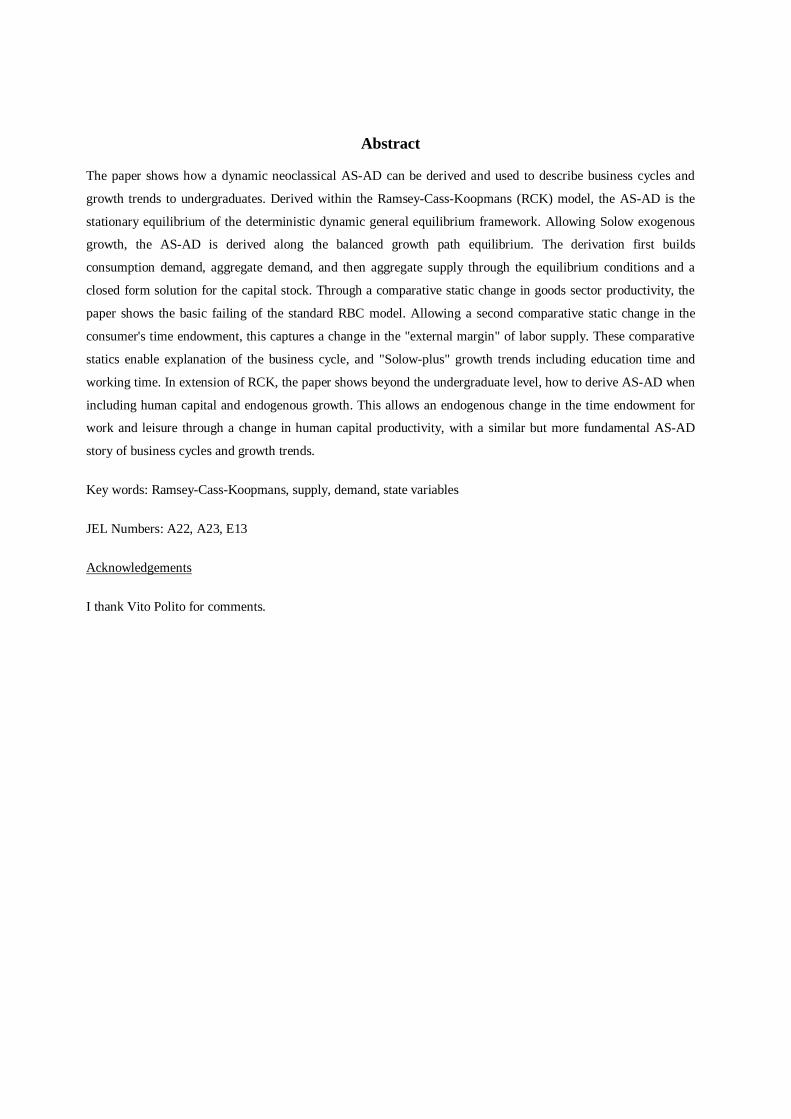
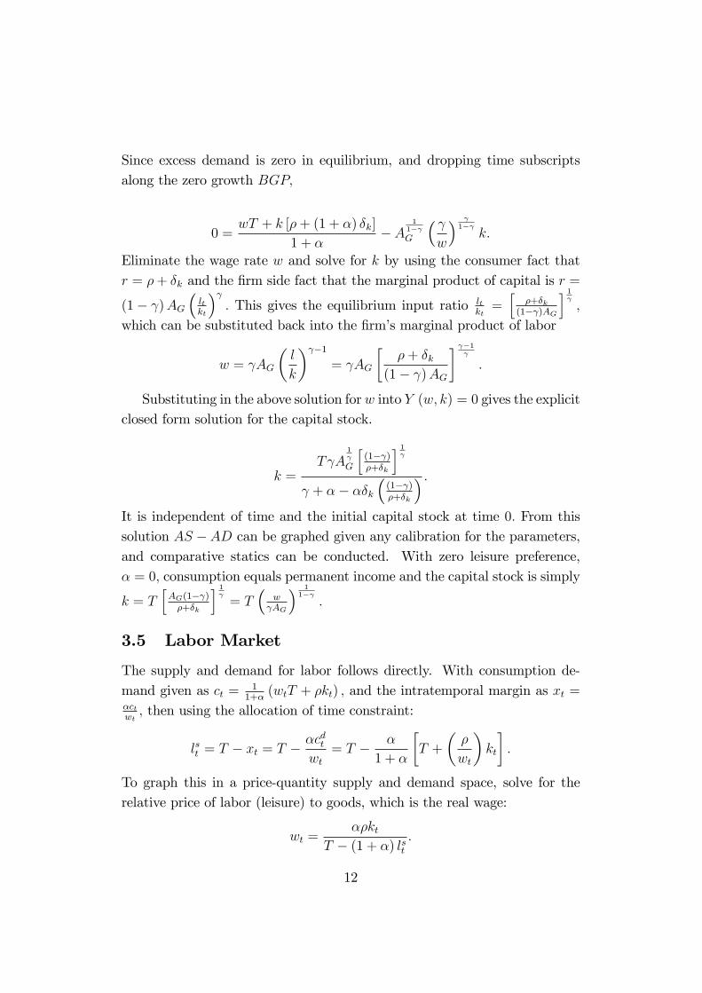
4.1 Example Calibration

Assume as in Gillman (2011) that = 13; � = 0:5; � = 0:03; T = 1; �k =

0:03 and AG = 0:15. Then the equilibrium capital stock will equal k =

13

0.0 0.1 0.2 0.3 0.40

5

10

15

Aggregate Output y

1/w

Figure 1: RCK AS � AD Equilibrium

(1)( 13)(0:15)3( 2

3(0:06))3

( 13+0:5)�0:5(0:03)(2

3(0:06))= 2:3148: The AD and AS are given respectively as

1

w=

1

yd (1 + 0:5)� 2:3148 [0:03 + (1:5) 0:03] ;

1

w=

(ys)2

13(0:15)3 (2:3148)2

:

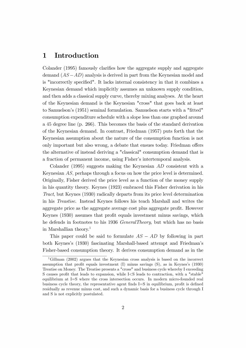
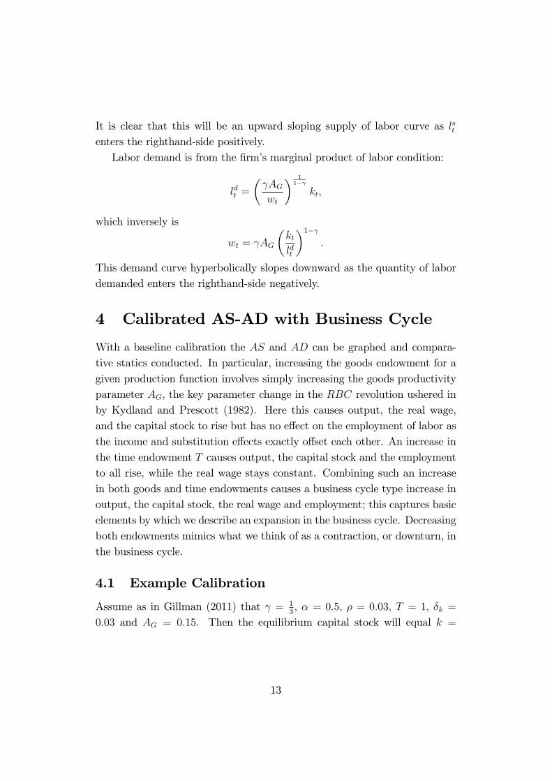
Figure 1 graphs these equations with the equilibrium wage of w = 0:138.Similarly the labor market equations are given by

w =0:5 (0:03) 2:3148

1� (1:5) ls ;

w =1

3(0:15)

�2:3148

ld

� 23

:

Figure 2 graphs these with an employment rate of 0:5:

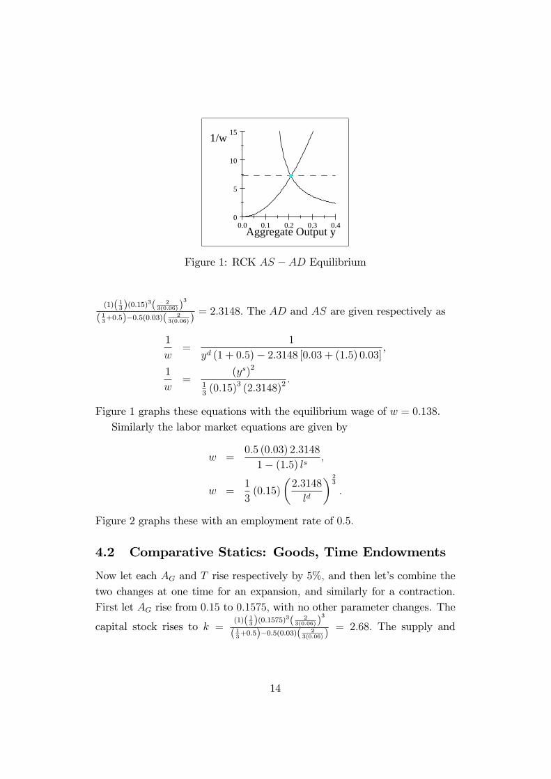
4.2 Comparative Statics: Goods, Time Endowments

Now let each AG and T rise respectively by 5%; and then let�s combine thetwo changes at one time for an expansion, and similarly for a contraction.First let AG rise from 0:15 to 0:1575; with no other parameter changes. The

capital stock rises to k =(1)( 13)(0:1575)

3( 23(0:06))

3

( 13+0:5)�0:5(0:03)(2

3(0:06))= 2:68: The supply and

14

0.0 0.2 0.4 0.6 0.8 1.00.0

0.1

0.2

0.3

Labor Supply and Demand

w

Figure 2: RCK Labor Market.

demand equations in the goods and labor markets become:

AD :1

w=

1

yd (1 + 0:5)� 2:68 [0:03 + (1:5) 0:03] ;

AS :1

w=

(ys)2

13(0:1575)3 (2:68)2

;

wt =(0:03) 2:68

1� (1:5) lst; wt =

1

3(0:1575)

�2:68

ld

� 23

:

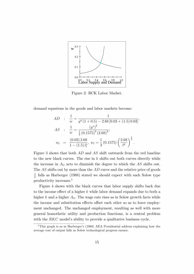
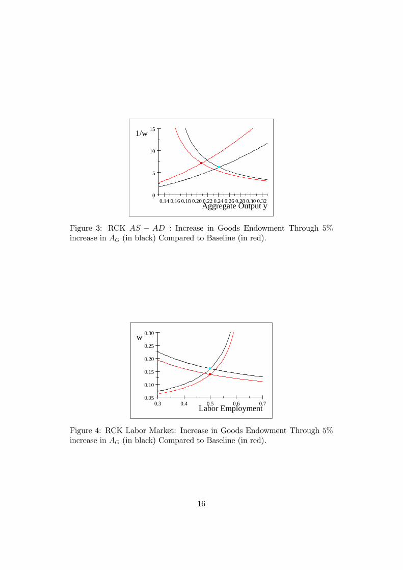
Figure 3 shows that both AD and AS shift outwards from the red baselineto the new black curves. The rise in k shifts out both curves directly whilethe increase in AG acts to diminish the degree to which the AS shifts out.The AS shifts out by more than the AD curve and the relative price of goods1wfalls as Harberger (1988) stated we should expect with such Solow type

productivity increases.5

Figure 4 shows with the black curves that labor supply shifts back dueto the income e¤ect of a higher k while labor demand expands due to both ahigher k and a higher AG: The wage rate rises as in Solow growth facts whilethe income and substitution e¤ects o¤set each other so as to leave employ-ment unchanged. The unchanged employment, resulting as well with moregeneral homothetic utility and production functions, is a central problemwith the RKC model�s ability to provide a qualitative business cycle.

5This graph is as in Harberger�s (1988) AEA Presidential address explaining how theaverage cost of output falls as Solow technological progress ensues.

15

0.14 0.16 0.18 0.20 0.22 0.24 0.26 0.28 0.30 0.320

5

10

15

Aggregate Output y

1/w

Figure 3: RCK AS � AD : Increase in Goods Endowment Through 5%increase in AG (in black) Compared to Baseline (in red).

0.3 0.4 0.5 0.6 0.70.05

0.10

0.15

0.20

0.25

0.30

Labor Employment

w

Figure 4: RCK Labor Market: Increase in Goods Endowment Through 5%increase in AG (in black) Compared to Baseline (in red).

16

0.18 0.20 0.22 0.245

6

7

8

9

10

Aggregate Output y

1/w

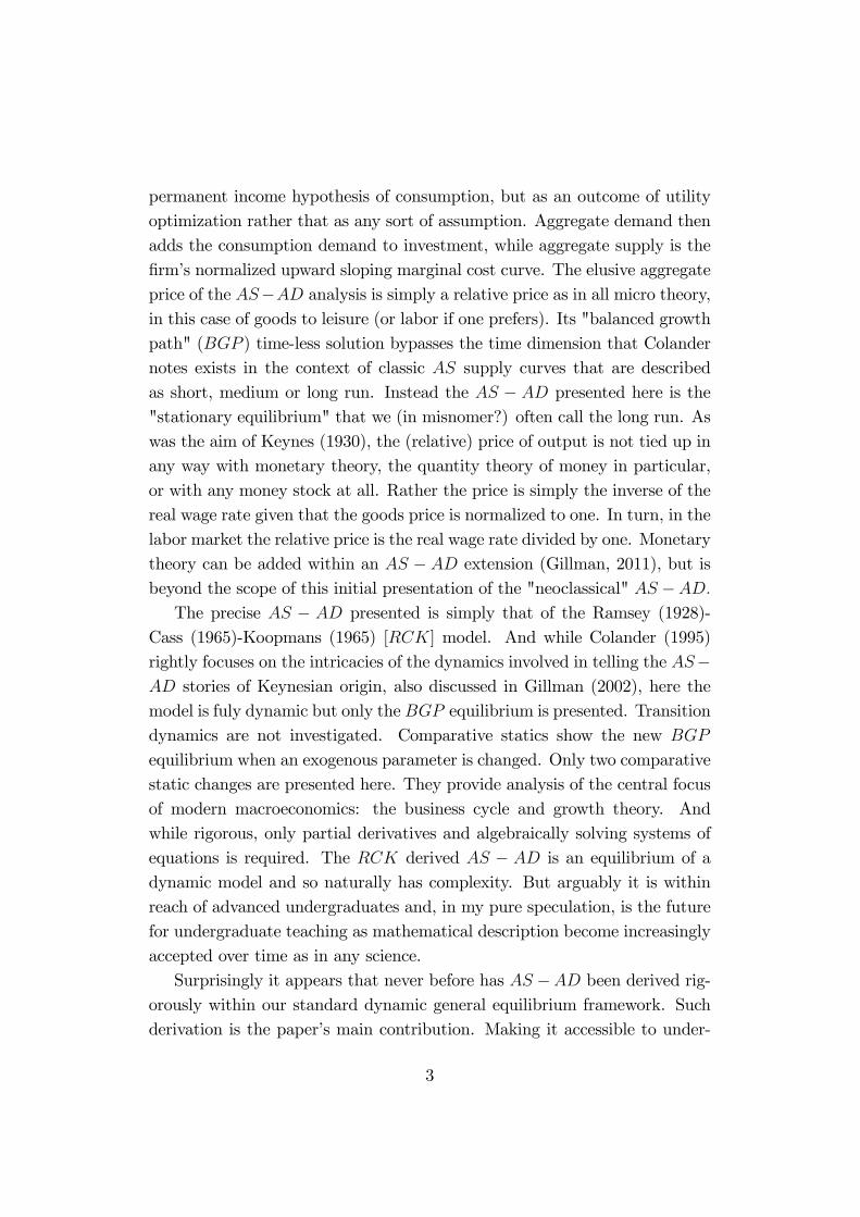
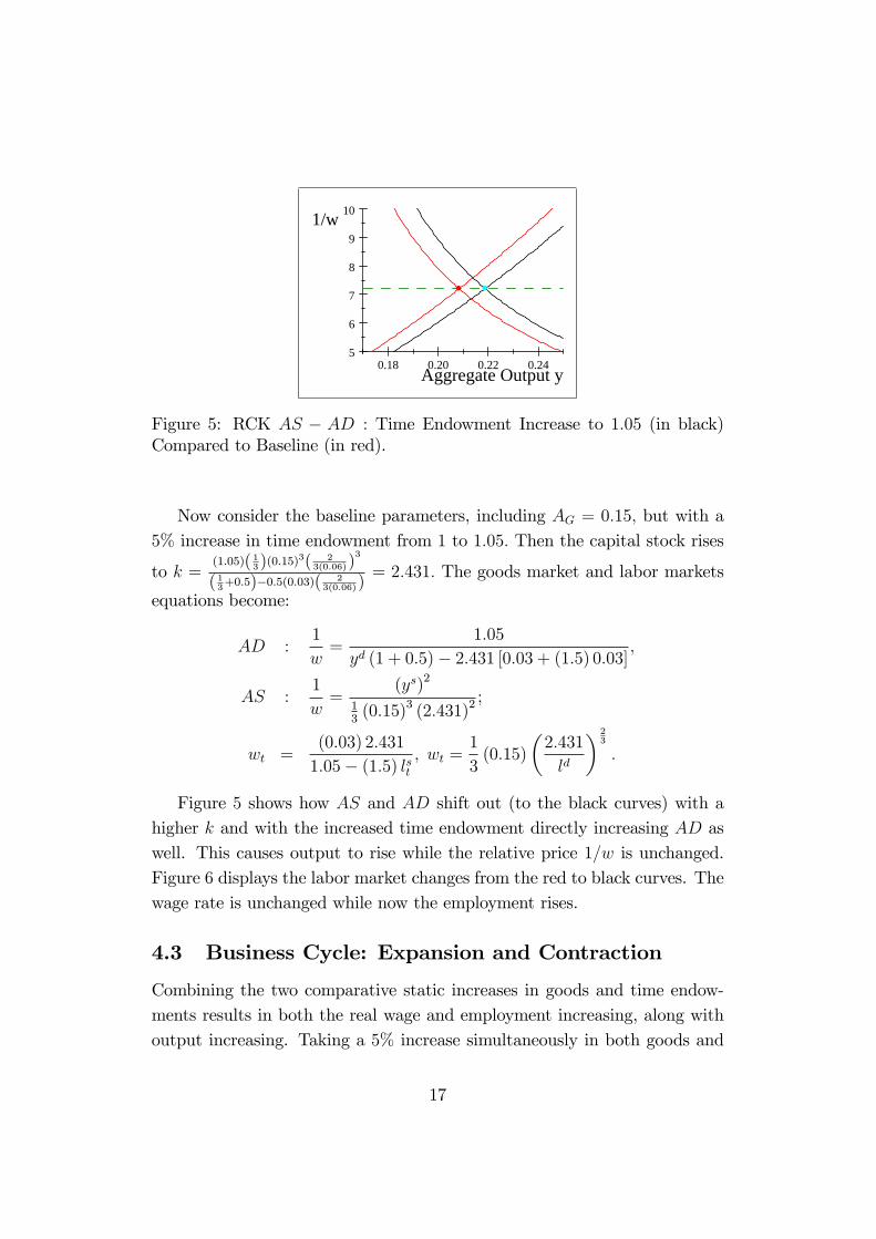
Figure 5: RCK AS � AD : Time Endowment Increase to 1:05 (in black)Compared to Baseline (in red).

Now consider the baseline parameters, including AG = 0:15; but with a5% increase in time endowment from 1 to 1:05: Then the capital stock rises

to k =(1:05)( 13)(0:15)

3( 23(0:06))

3

( 13+0:5)�0:5(0:03)(2

3(0:06))= 2:431: The goods market and labor markets

equations become:

AD :1

w=

1:05

yd (1 + 0:5)� 2:431 [0:03 + (1:5) 0:03] ;

AS :1

w=

(ys)2

13(0:15)3 (2:431)2

;

wt =(0:03) 2:431

1:05� (1:5) lst; wt =

1

3(0:15)

�2:431

ld

� 23

:

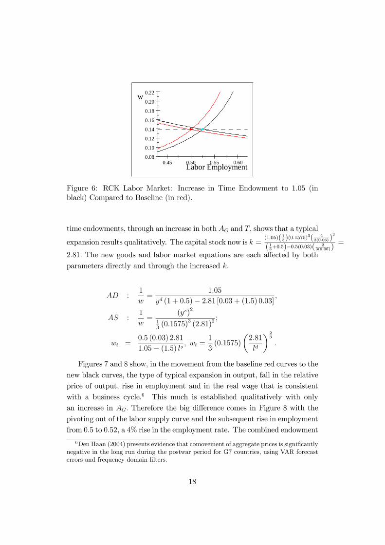
Figure 5 shows how AS and AD shift out (to the black curves) with ahigher k and with the increased time endowment directly increasing AD aswell. This causes output to rise while the relative price 1=w is unchanged.Figure 6 displays the labor market changes from the red to black curves. Thewage rate is unchanged while now the employment rises.

4.3 Business Cycle: Expansion and Contraction

Combining the two comparative static increases in goods and time endow-ments results in both the real wage and employment increasing, along withoutput increasing. Taking a 5% increase simultaneously in both goods and

17

0.45 0.50 0.55 0.600.08

0.10

0.12

0.14

0.16

0.18

0.20

0.22

Labor Employment

w

Figure 6: RCK Labor Market: Increase in Time Endowment to 1:05 (inblack) Compared to Baseline (in red).

time endowments, through an increase in both AG and T; shows that a typical

expansion results qualitatively. The capital stock now is k =(1:05)( 13)(0:1575)

3( 23(0:06))

3

( 13+0:5)�0:5(0:03)(2

3(0:06))=

2:81: The new goods and labor market equations are each a¤ected by bothparameters directly and through the increased k:

AD :1

w=

1:05

yd (1 + 0:5)� 2:81 [0:03 + (1:5) 0:03] ;

AS :1

w=

(ys)2

13(0:1575)3 (2:81)2

;

wt =0:5 (0:03) 2:81

1:05� (1:5) ls ; wt =1

3(0:1575)

�2:81

ld

� 23

:

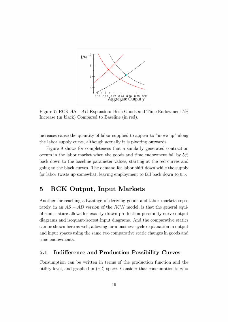
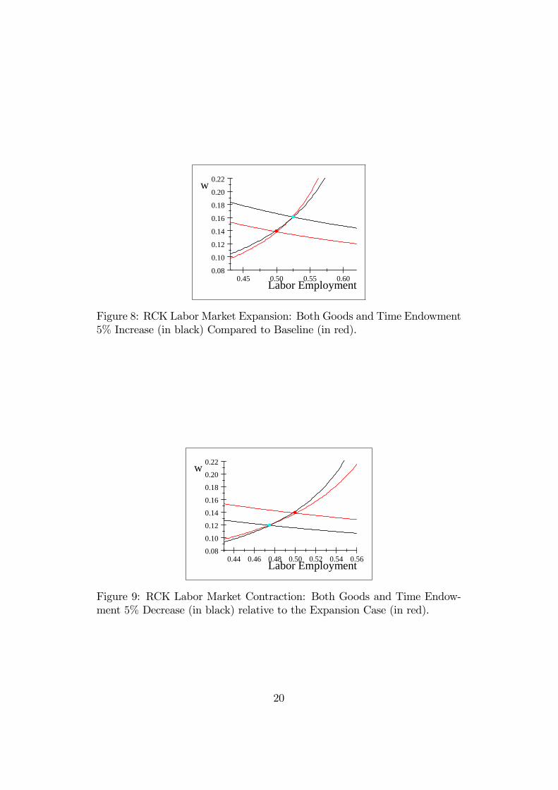
Figures 7 and 8 show, in the movement from the baseline red curves to thenew black curves, the type of typical expansion in output, fall in the relativeprice of output, rise in employment and in the real wage that is consistentwith a business cycle.6 This much is established qualitatively with onlyan increase in AG: Therefore the big di¤erence comes in Figure 8 with thepivoting out of the labor supply curve and the subsequent rise in employmentfrom 0:5 to 0:52, a 4% rise in the employment rate. The combined endowment

6Den Haan (2004) presents evidence that comovement of aggregate prices is signi�cantlynegative in the long run during the postwar period for G7 countries, using VAR forecasterrors and frequency domain �lters.

18

0.18 0.20 0.22 0.24 0.26 0.28 0.30

4

6

8

10

Aggregate Output y

1/w

Figure 7: RCK AS�AD Expansion: Both Goods and Time Endowment 5%Increase (in black) Compared to Baseline (in red).

increases cause the quantity of labor supplied to appear to "move up" alongthe labor supply curve, although actually it is pivoting outwards.Figure 9 shows for completeness that a similarly generated contraction

occurs in the labor market when the goods and time endowment fall by 5%back down to the baseline parameter values, starting at the red curves andgoing to the black curves. The demand for labor shift down while the supplyfor labor twists up somewhat, leaving employment to fall back down to 0:5:

5 RCK Output, Input Markets

Another far-reaching advantage of deriving goods and labor markets sepa-rately, in an AS � AD version of the RCK model, is that the general equi-librium nature allows for exactly drawn production possibility curve outputdiagrams and isoquant-isocost input diagrams. And the comparative staticscan be shown here as well, allowing for a business cycle explanation in outputand input spaces using the same two comparative static changes in goods andtime endowments.

5.1 Indi¤erence and Production Possibility Curves

Consumption can be written in terms of the production function and theutility level, and graphed in (c; l) space. Consider that consumption is cdt =

19

0.45 0.50 0.55 0.600.08

0.10

0.12

0.14

0.16

0.18

0.20

0.22

Labor Employment

w

Figure 8: RCK Labor Market Expansion: Both Goods and Time Endowment5% Increase (in black) Compared to Baseline (in red).

0.44 0.46 0.48 0.50 0.52 0.54 0.560.08

0.10

0.12

0.14

0.16

0.18

0.20

0.22

Labor Employment

w

Figure 9: RCK Labor Market Contraction: Both Goods and Time Endow-ment 5% Decrease (in black) relative to the Expansion Case (in red).

20

yst � it = AG�ldt� (kt)

1� � �kkt: Substituting in the baseline parameters,k = 2:315; and AG = 0:15; this gives a "production possibility curve" (PPC)of

cdt = 0:262�ldt� 13 � 0:069:

Similarly, the utility level can be found in the baseline as ln ct+� ln (1� lt) =ln 0:13889 + 0:5 ln 0:5 = �2:32: Solving for ct; the indi¤erence curve at thenew equilibrium after the AG increase is

ct =e�2:32

(1� lt)0:5:

The budget line in equilibrium is

cdt = wtlst + �kt = c

dt = (0:13889) l

st + (0:03) (2:3148) :

It is worth pointing out the symmetry of the budget line between bothconsumer and �rm. In fact, the consumer�s budget line here is the sameline as the �rm�s pro�t line in the BGP equilibrium. For the �rm yt =

wtlt + rtkt; and since rt = � + �k; then yt = wtlt + (�+ �k) kt: Given alsothat output equals consumption plus investment, yt = ct+ it; and that BGPinvestment equals the maintenance for capital depreciation, or it = �kkt; thenconsumption as solved for from the �rm�s pro�t de�nition is ct = yt � it =wtl

dt +(�+ �k) kt� �kkt; or ct = wtldt + �kt:With labor supply equal to labor

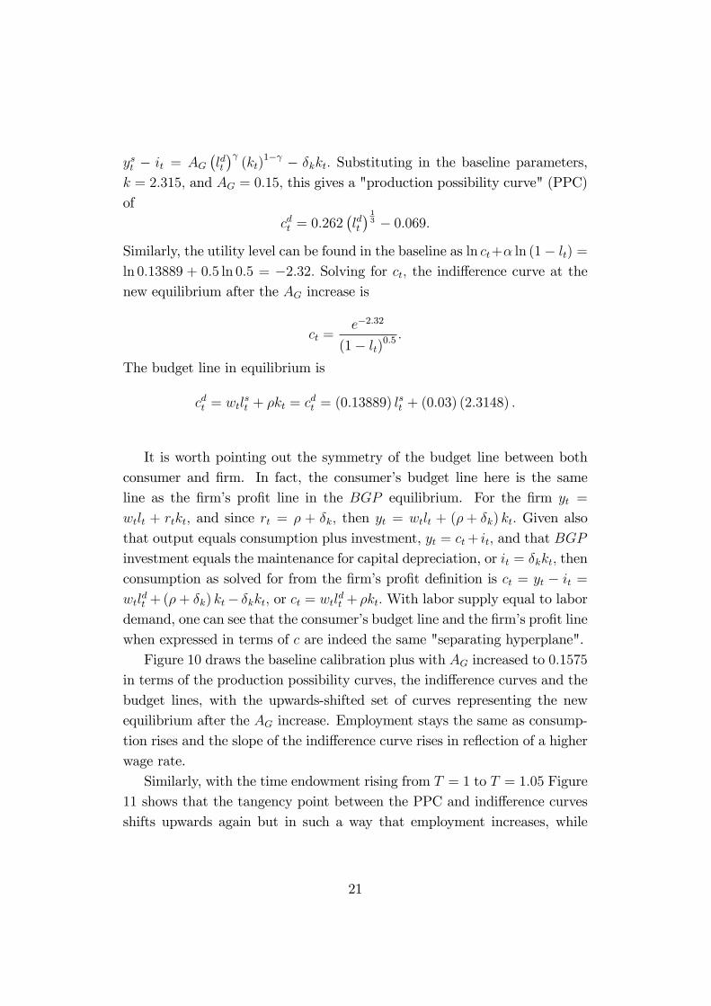
demand, one can see that the consumer�s budget line and the �rm�s pro�t linewhen expressed in terms of c are indeed the same "separating hyperplane".Figure 10 draws the baseline calibration plus with AG increased to 0:1575

in terms of the production possibility curves, the indi¤erence curves and thebudget lines, with the upwards-shifted set of curves representing the newequilibrium after the AG increase. Employment stays the same as consump-tion rises and the slope of the indi¤erence curve rises in re�ection of a higherwage rate.Similarly, with the time endowment rising from T = 1 to T = 1:05 Figure

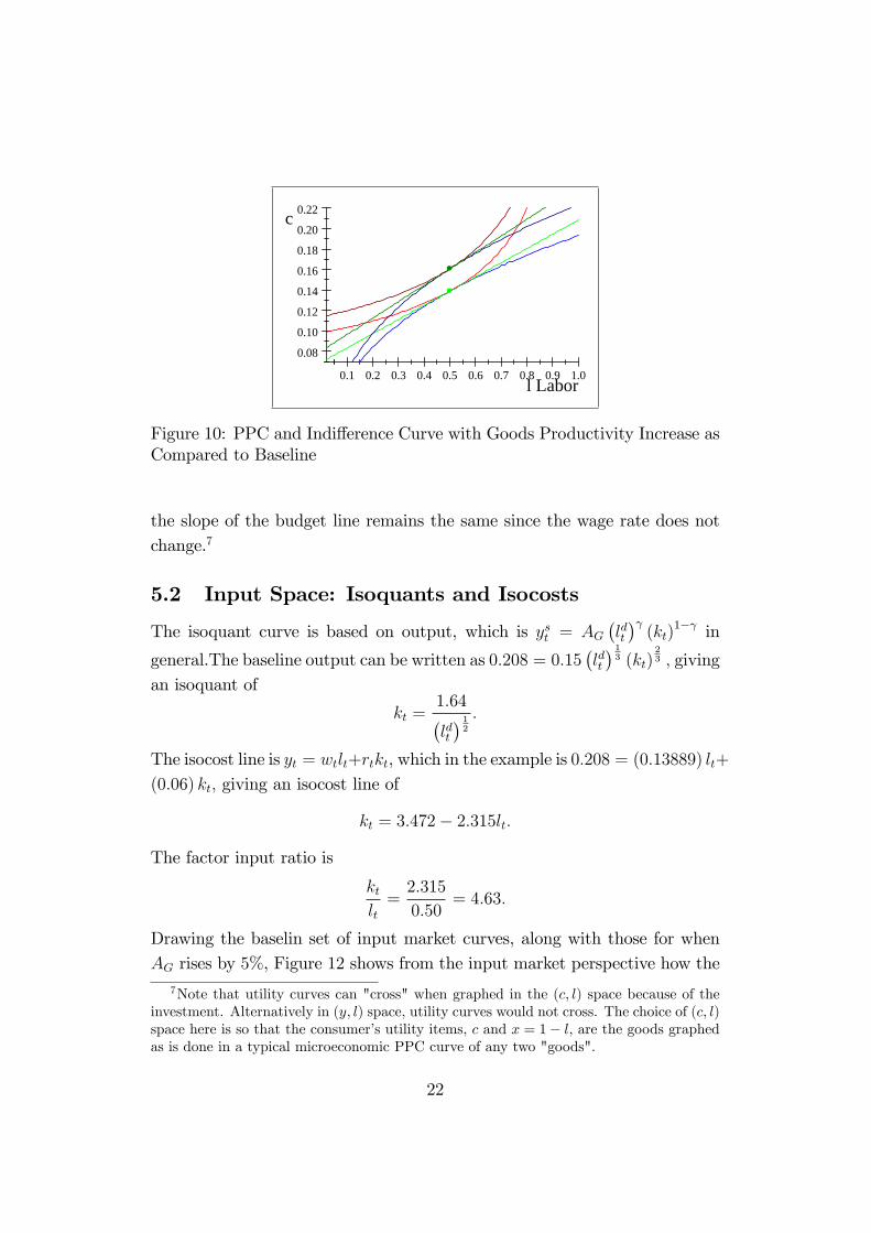
11 shows that the tangency point between the PPC and indi¤erence curvesshifts upwards again but in such a way that employment increases, while

21

0.1 0.2 0.3 0.4 0.5 0.6 0.7 0.8 0.9 1.0

0.08

0.10

0.12

0.14

0.16

0.18

0.20

0.22

l Labor

c

Figure 10: PPC and Indi¤erence Curve with Goods Productivity Increase asCompared to Baseline

the slope of the budget line remains the same since the wage rate does notchange.7

5.2 Input Space: Isoquants and Isocosts

The isoquant curve is based on output, which is yst = AG�ldt� (kt)

1� in

general.The baseline output can be written as 0:208 = 0:15�ldt� 13 (kt)

23 ; giving

an isoquant of

kt =1:64�ldt� 12

:

The isocost line is yt = wtlt+rtkt, which in the example is 0:208 = (0:13889) lt+(0:06) kt; giving an isocost line of

kt = 3:472� 2:315lt:

The factor input ratio is

ktlt=2:315

0:50= 4:63:

Drawing the baselin set of input market curves, along with those for whenAG rises by 5%, Figure 12 shows from the input market perspective how the

7Note that utility curves can "cross" when graphed in the (c; l) space because of theinvestment. Alternatively in (y; l) space, utility curves would not cross. The choice of (c; l)space here is so that the consumer�s utility items, c and x = 1� l; are the goods graphedas is done in a typical microeconomic PPC curve of any two "goods".

22

0.3 0.4 0.5 0.6 0.7

0.11

0.12

0.13

0.14

0.15

0.16

0.17

l Labor

c

Figure 11: PPC and Indi¤erence Curves with Time Endowment Increase asCompared to Baseline.

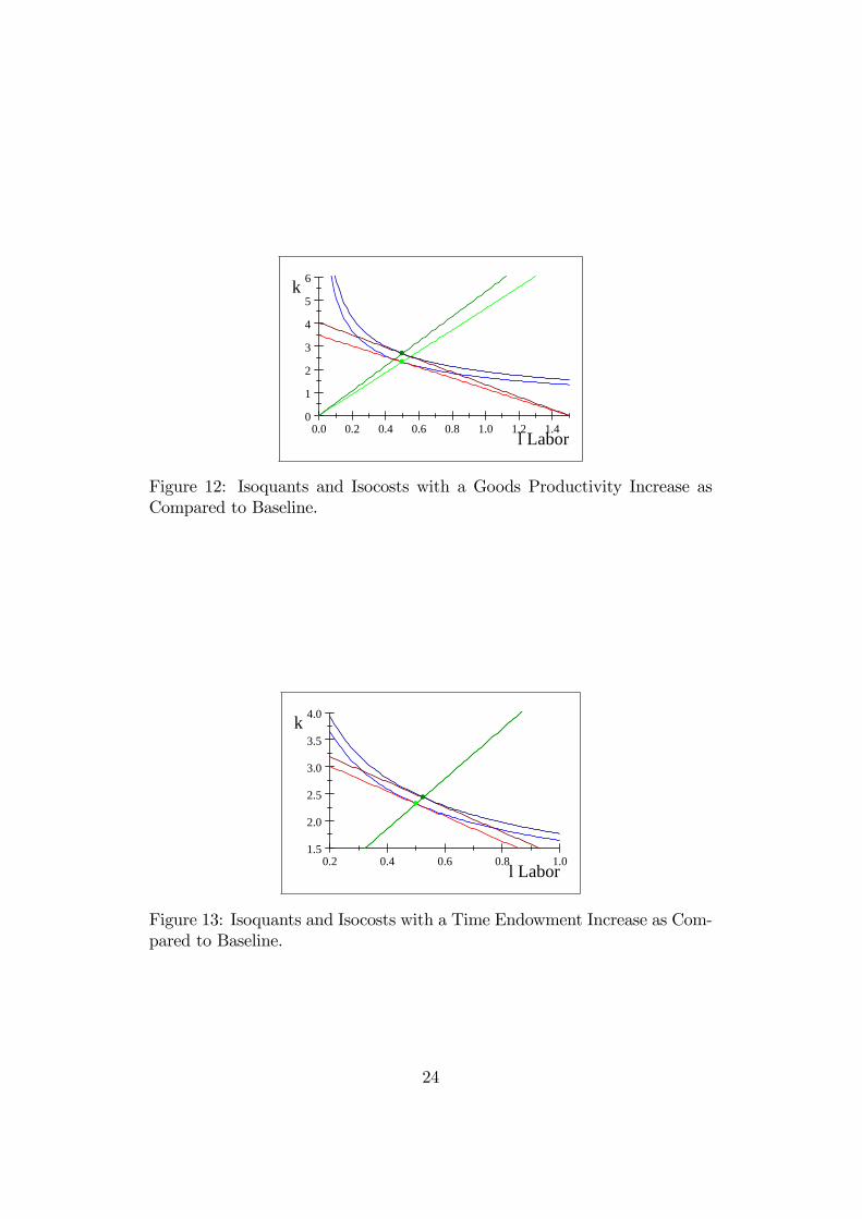
increase in AG causes the equilibrium isoquant to shift up, employment toremain the same and the input ratio k=l to pivot up; a steeper isocost showsthe higher real wage.For the increase in the time endowment to T = 1:05; Figure 13 re�ects

that the factor input ratio remains the same (an identical input ratio forany T ) as the equilibrium isoquant shifts up and employment rises, as com-pared to the baseline. The same sloped isocost re�ects that factor prices areunchanged.Simultaneously increasing the goods and time endowments as in a busi-

ness cycle expansion would result in similar output and input market graphs.The "production possibility curve" would pivot upwards with an increasedslope of the consumer-budget/�rm-pro�t line at the tangency with the newhigher indi¤erence curve, as the real wage, output and labor employment rise.And in the input market the isoquant would shift out and the isocost pivotupwards such that again a higher real wage, output level, and employmentwould be shown.

6 Exogenous Growth Theory

Allowing the goods sector productivity factor AG to rise at a constant rate ofgrowth gives all of Solow�s growth facts in the RCK model. And it is easilyillustrated in both the goods market, using AS � AD analysis, and in the

23

0.0 0.2 0.4 0.6 0.8 1.0 1.2 1.40

1

2

3

4

5

6

l Labor

k

Figure 12: Isoquants and Isocosts with a Goods Productivity Increase asCompared to Baseline.

0.2 0.4 0.6 0.8 1.01.5

2.0

2.5

3.0

3.5

4.0

l Labor

k

Figure 13: Isoquants and Isocosts with a Time Endowment Increase as Com-pared to Baseline.

24

labor market. Letting AG grow at a constant rate �;

AGt+1 = AGt (1 + �) :

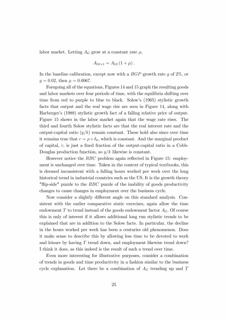
In the baseline calibration, except now with a BGP growth rate g of 2%; org = 0:02; then � = 0:0067:Foregoing all of the equations, Figures 14 and 15 graph the resulting goods

and labor markets over four periods of time; with the equilibria shifting overtime from red to purple to blue to black. Solow�s (1965) stylistic growthfacts that output and the real wage rise are seen in Figure 14, along withHarberger�s (1988) stylistic growth fact of a falling relative price of output.Figure 15 shows in the labor market again that the wage rate rises. Thethird and fourth Solow stylistic facts are that the real interest rate and theoutput-capital ratio (y=k) remain constant. These hold also since over timeit remains true that r = �+�k; which is constant. And the marginal productof capital, r; is just a �xed fraction of the output-capital ratio in a Cobb-Douglas production function, so y=k likewise is constant.However notice the RBC problem again re�ected in Figure 15: employ-

ment is unchanged over time. Taken in the context of typical textbooks, thisis deemed inconsistent with a falling hours worked per week over the longhistorical trend in industrial countries such as the US. It is the growth theory"�ip-side" puzzle to the RBC puzzle of the inability of goods productivitychanges to cause changes in employment over the business cycle.Now consider a slightly di¤erent angle on this standard analysis. Con-

sistent with the earlier comparative static exercises, again allow the timeendowment T to trend instead of the goods endowment factor AG: Of coursethis is only of interest if it allows additional long run stylistic trends to beexplained that are in addition to the Solow facts. In particular, the declinein the hours worked per week has been a centuries old phenomenon. Doesit make sense to describe this by allowing less time to be devoted to workand leisure by having T trend down, and employment likewise trend down?I think it does, as this indeed is the result of such a trend over time.Even more interesting for illustrative purposes, consider a combination

of trends in goods and time productivity in a fashion similar to the businesscycle explanation. Let there be a combination of AG trending up and T

25

0.23 0.24 0.25 0.26 0.27 0.285

6

7

8

9

10

Aggregate Output y

1/w

Figure 14: AS � AD Equilibria Over Four Periods with a BGP ExogenousGrowth Rate of g = 0:02.

0.590 0.595 0.600 0.605 0.610

0.135

0.140

0.145

0.150

0.155

0.160

Labor

w

Figure 15: Labor Market with 2% Exogenous Growth:

26

0.590 0.595 0.600 0.605 0.610

0.135

0.140

0.145

0.150

0.155

0.160

Labor

w

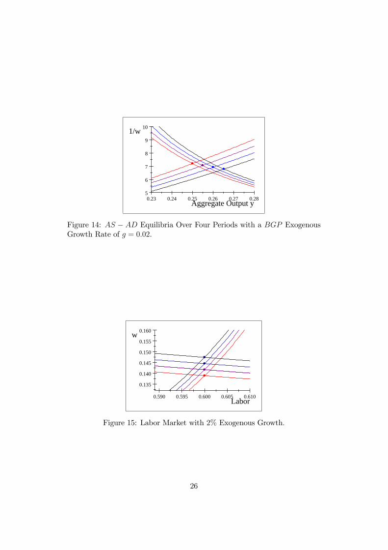
Figure 16: Labor Market with AG Trending Up and T Trending Down:

trending down slightly, as presented in both the goods and labor markets.8

The goods market qualitatively looks like Figure 14 and so will not be repro-duced; 1=w falls as output rises. However in Figure 16 the labor market isshown to reproduce a rising wage rate along with a very gradually decliningtrend in time spent working, as the equilibria over time again go from thered to purple to blue and to the black in the most recent time period. Allof these trending equilibria can also be shown in the PPC-indi¤erence curvespace and the factor input space, although those graphs are foregone here forsimplicity of presentation.The idea is to capture the trend downwards in the work week by account-

ing for the trend upwards in time spent in education, over the centuries. Inother words, it is plausible that our lifetime allocation of time for work andleisure has fallen over time as our education time has gradually trended up.For example, looking at the time since the industrial revolution began in the1700s, average education levels have gone from no primary school to someyears in primary, to some in high school, to a high school diploma average,to some university years, to a bachelors degree, etc.Capturing a fall in T is here a representation of how education time has

increased, although this is not explained explicitly within the RCK modelor one with Solow exogenous growth. However an increase in education timeand a consequent fall in T can be made endogenous by extending the Solow

8The trend down in T is 0:00182 per year, based on evidence reporting a 12% decreasein US labor time from 1965 to 2005, in Aguiar and Hurst (2009).

27

model as did Lucas (1988) through an additional sector for investment inhuman capital.

7 Endogenous Growth and Business Cycles

Thus far the modelling approach, themes of business cycles and growth, andmathematical sophistication is within reach of advanced undergraduates, orthose even at an intermediate level if they have a good grasp of partialderivatives, solving systems of equations, and economic intuition. All thesolutions have been closed-form analytic ones. Going one step further, toendogenize growth through human capital investment, can still be done usingAS � AD; only partial derivatives and solving systems of equations, andall within a closed form solution. However now the solution involves is aquadratic which has a closed form explicit solution, but obviously is morecomplex looking and may be accessible for only the most mathematicallyinclined undergraduates. At this point, the material arguably becomes moreof a masters level, or �rst PhD course level.Here I will present the extension brie�y, as it is relatively simple and it

provides the key to how T is changed endogenously, rather than exogenouslyin the work up until now. This is important because the only additional com-parative static beyond the typical goods productivity has been this change inT: In the RBC and Solow-growth fashion of changing productivity parame-ters, when the productivity parameter of the human capital sector is changed,the time that the representative agent devotes to education changes and thisin turn endogenously changes the time left-over for goods and leisure, or T:This provides understanding that the change in T in the RCK model is notan arbitrary arti�ce by which to describe cycles and growth. The change inT with endogenous growth results from a sectoral productivity change in theeducation sector. In di¤erent terms, this is like changing the productivityof the "non-market" sector in the two sector business cycle theory begun inparticular with Benhabib et al. (1991) and Greenwood and Hercowitz (1991),after evolving from Hansen (1985) and Rogerson (1988). But now the addi-tional non-market sector is the sector producing human capital investmentin a costly Lucas (1988) fashion.Besides consistency with adding greater labor volatility in the RBC lit-

28

erature by adding an external labor margin, the extension in turn explainsan important additional trend explicitly: the rise in lifetime education timethrough a trend up in human capital sectoral productivity. This also is arather simple way to explain how the BGP growth rate can rise over time,as has indeed been witnessed in the last 250 years at the same time as edu-cation time has trended upwards. Therefore these two additional trends ineducation and the growth rate are explained in a very simple fashion througha trend up in the productivity parameter in the Lucas (1988) human capitalinvestment sector.

7.1 The Human Capital Extension

With ht denoting human capital, the goods sector production function nowis

yst = AG�ldt ht

� (kt)

1� ;

so that the change relative to the RCK with Solow growth is to think ofAGt now being de�ned instead as an AGt � AG (ht) : Instead of exogenoustechnological change in AG; there is endogenous change in AGt as a result ofthe consumer�s choice of human capital.The new sector for producing human capital investment is given by

ht+1 = ht (1� �h) + iht;

where �h 2 [0; 1] is the depreciation rate of human capital and iht is a the sec-toral investment function given by a simple linear (Lucas, 1988) productionfunction:

iht = AH lHtht;

in which AH is the sectoral productivity parameter, and lHt the fraction oftime spent accumulating human capital. In short, ht+1 = ht (1 + AH lHt � �H).Time allocation now includes not just labor and leisure, which will still bedenoted in sum as T; but also the time lht devoted to "education":

1 = T + lht = lst + xt + lht:

The time T becomes endogenous as more or less time goes into producinghuman capital.

29

The consumer problem becomes

V (kt; ht) = Maxkt+1;ht_1;lst ;lHt;xt

: ln [wtlstht + rtkt � kt+1 + kt � �kkt] + � ln (xt)

+�V (kt+1; ht+1) ;

subject to ht+1 = ht (1� �h) + AH lhtht and 1 = lst + xt + lHt; where ct =wtl

stht+rtkt�kt+1+kt��kkt: Note that the only di¤erence in the goods budget

constraint is that wages are indexed by the human capital of the consumer,being equal to wtlstht instead of wtl

st : Substituting in the constraints, the

consumer problem is9

V (kt; ht) = Maxkt+1;lst ;lHt;

: ln [wtlstht + rtkt � kt+1 + kt � �kkt] + � ln (1� lHt � lst )

+�V [kt+1; ht (1� �h) + AH lHtht] :

Along the BGP the intratemporal goods-leisure margin (MRSc;x :�cdtxt=

wtht), and the physical capital intertemporal margin�1 + gt =

1+rt��k1+�

�are

joined by the human capital intertemporal margin: 1 + gt =1+AH(1�xt)��h

1+�:

The growth rate become endogenous by virtue of the consumer�s choice ofleisure xt: More leisure means a lower "human capital capacity utilizationrate" of 1 � xt, and a lower return on human capital. Since the BGP seesequivalence of capital returns, rt� �k = AH (1� xt)� �h: If leisure increasesand so the productively employed time (lst+lHt) decreases, then also it followsthat rt falls. This happens by increasing physical capital relative to human

9The equilibrium and envelope conditions are

kt+1 :1

cdt(�1) + � @V (kt+1; ht+1)

@kt+1= 0;

lst :1

cdt(wtht) +

�

xt(�1) = 0;

lHt :�

xt(�1) + � @V (kt+1; ht+1)

@ht+1(AHht) = 0;

kt :@V (kt; ht)

@kt=1

cdt(1 + rt � �k) ;

ht :@V (kt; ht)

@ht=1

cdt(wtlt) + �

@V (kt+1; ht+1)

@ht+1(1 +AH lHt � �H) :

ht :@V (kt; ht)

@ht=1

cdt(wtlt) + �

@V (kt+1; ht+1)

@ht+1(1 +AH lHt � �H) :

30

capital, since the return to human capital has fallen. In this environment, thenew "state" variable along the BGP is indeed the ratio k=h: A decrease inAH causes less lHt, more leisure, and a higher k=h as the consumer substitutesfrom human to physical capital.

7.2 Extended AS-AD

The consumer demand function can now be solved with the addition thattime in human capital accumulation enters it. Following similar steps to theabove derivation of consumer demand, now

cdt =1

1 + �[wtht (1� lHt) + kt (rt � �k � g)] :

Using the human capital investment and its BGP condition that 1 + g =ht+1ht

= 1 + AH lHt � �H ; we can write human capital time as lHt = g+�HAH

:

Stationary consumption is written as normalized by human capital ht; wherekthtis constant in the BGP equilibrium:

cdtht=

1

1 + �

�wt

�1� g + �H

AH

�+ktht� (1 + g)

�:

In terms of the permanent income hypothesis of consumption, now cdt =�1

1+�

�yPt where yPt can be written as yPt = wthtTt + kt� (1 + g) ; similar to

the RCK model with a positive g except for the indexing of wage income byht:

Investment with a positive growth rate g is (g + �k) kt: Adding this toconsumer demand and normalizing by ht gives aggregate demand.

AD :ydtht=

1

1 + �

�wt

�1� g + �H

AH

�+ktht[� (1 + g) + (g + �k) (1 + �)]

�;

1

wt=

1� g+�HAH

ydtht(1 + �)� kt

ht[� (1 + g) + (g + �k) (1 + �)]

:

Aggregate supply ends up completely unchanged as yst = AG

� AGwt

� 1� kt;

which can be made stationary through normalization by ht :

AS :ystht= AG

� AGwt

� 1� kt

ht;1

wt=

1

AG

�ystAGkt

� 1�

:

31

0.0 0.1 0.2 0.3 0.40

5

10

y/h Aggregate Output

1/w

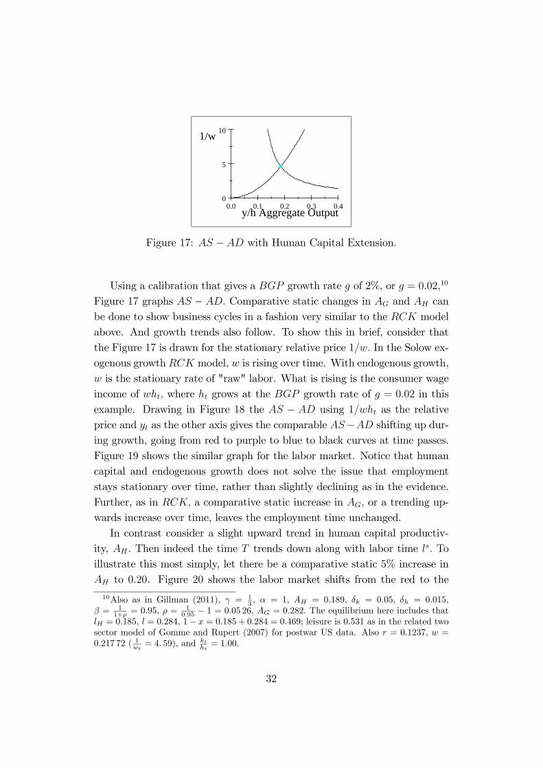
Figure 17: AS � AD with Human Capital Extension.

Using a calibration that gives a BGP growth rate g of 2%, or g = 0:02,10

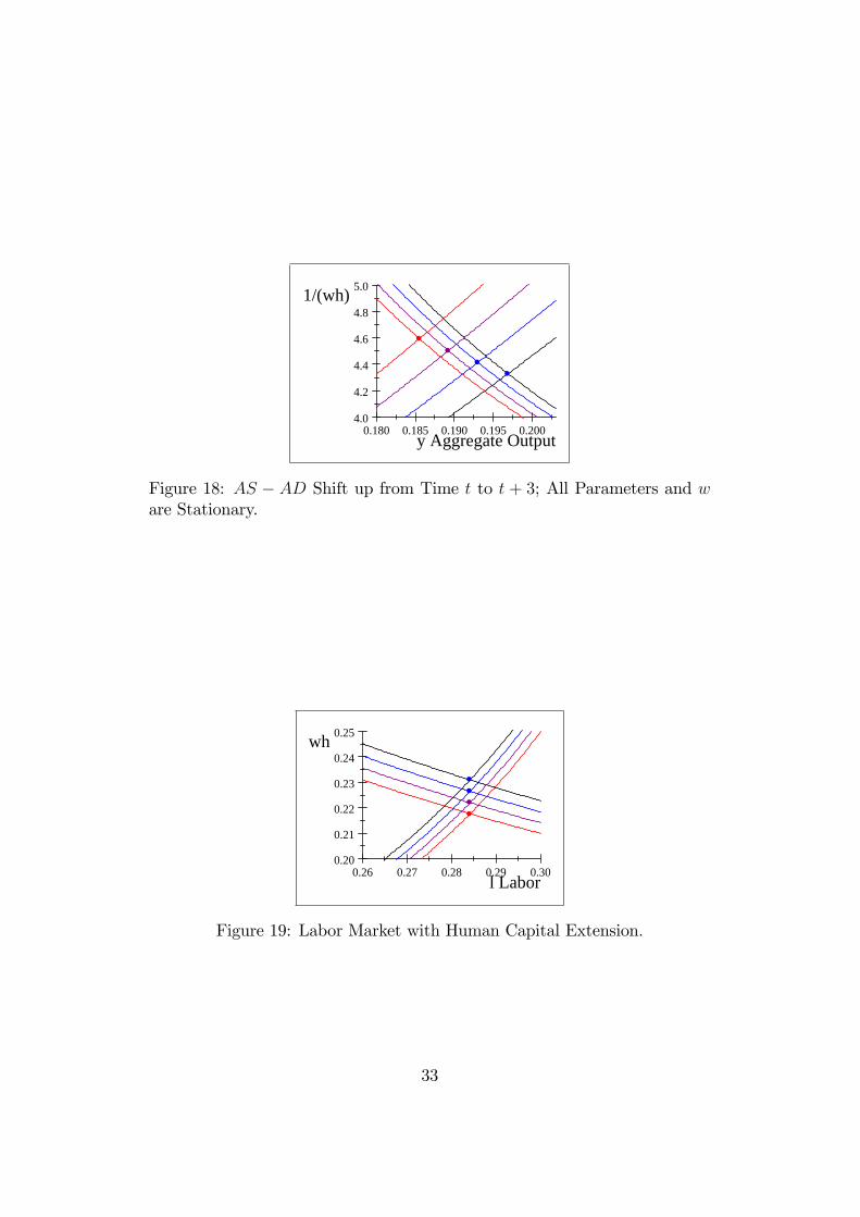
Figure 17 graphs AS � AD: Comparative static changes in AG and AH canbe done to show business cycles in a fashion very similar to the RCK modelabove. And growth trends also follow. To show this in brief, consider thatthe Figure 17 is drawn for the stationary relative price 1=w: In the Solow ex-ogenous growth RCK model, w is rising over time. With endogenous growth,w is the stationary rate of "raw" labor. What is rising is the consumer wageincome of wht; where ht grows at the BGP growth rate of g = 0:02 in thisexample. Drawing in Figure 18 the AS � AD using 1=wht as the relativeprice and yt as the other axis gives the comparable AS�AD shifting up dur-ing growth, going from red to purple to blue to black curves at time passes.Figure 19 shows the similar graph for the labor market. Notice that humancapital and endogenous growth does not solve the issue that employmentstays stationary over time, rather than slightly declining as in the evidence.Further, as in RCK; a comparative static increase in AG; or a trending up-wards increase over time, leaves the employment time unchanged.In contrast consider a slight upward trend in human capital productiv-

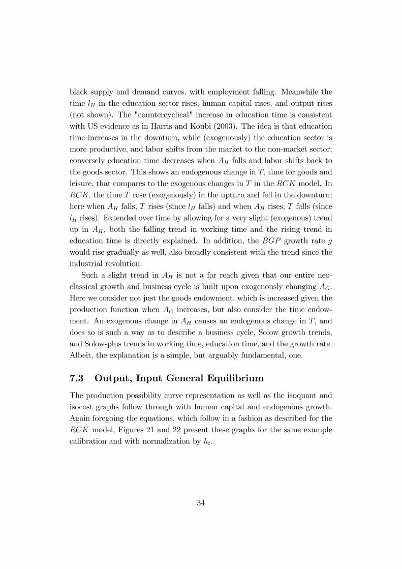
ity, AH : Then indeed the time T trends down along with labor time ls: Toillustrate this most simply, let there be a comparative static 5% increase inAH to 0:20. Figure 20 shows the labor market shifts from the red to the

10Also as in Gillman (2011), = 13 , � = 1; AH = 0:189; �k = 0:05; �h = 0:015;

� = 11+� = 0:95; � =

10:95 � 1 = 0:05 26; AG = 0:282: The equilibrium here includes that

lH = 0:185; l = 0:284; 1� x = 0:185 + 0:284 = 0:469; leisure is 0:531 as in the related twosector model of Gomme and Rupert (2007) for postwar US data. Also r = 0:1237; w =0:217 72 ( 1wt = 4: 59); and

ktht= 1:00:

32

0.180 0.185 0.190 0.195 0.2004.0

4.2

4.4

4.6

4.8

5.0

y Aggregate Output

1/(wh)

Figure 18: AS � AD Shift up from Time t to t + 3; All Parameters and ware Stationary.

0.26 0.27 0.28 0.29 0.300.20

0.21

0.22

0.23

0.24

0.25

l Labor

wh

Figure 19: Labor Market with Human Capital Extension:

33

black supply and demand curves, with employment falling. Meanwhile thetime lH in the education sector rises, human capital rises, and output rises(not shown). The "countercyclical" increase in education time is consistentwith US evidence as in Harris and Koubi (2003). The idea is that educationtime increases in the downturn, while (exogenously) the education sector ismore productive, and labor shifts from the market to the non-market sector;conversely education time decreases when AH falls and labor shifts back tothe goods sector. This shows an endogenous change in T; time for goods andleisure, that compares to the exogenous changes in T in the RCK model. InRCK; the time T rose (exogenously) in the upturn and fell in the downturn;here when AH falls, T rises (since lH falls) and when AH rises, T falls (sincelH rises). Extended over time by allowing for a very slight (exogenous) trendup in AH ; both the falling trend in working time and the rising trend ineducation time is directly explained. In addition, the BGP growth rate gwould rise gradually as well, also broadly consistent with the trend since theindustrial revolution.Such a slight trend in AH is not a far reach given that our entire neo-

classical growth and business cycle is built upon exogenously changing AG:Here we consider not just the goods endowment, which is increased given theproduction function when AG increases, but also consider the time endow-ment. An exogenous change in AH causes an endogenous change in T; anddoes so is such a way as to describe a business cycle, Solow growth trends,and Solow-plus trends in working time, education time, and the growth rate.Albeit, the explanation is a simple, but arguably fundamental, one.

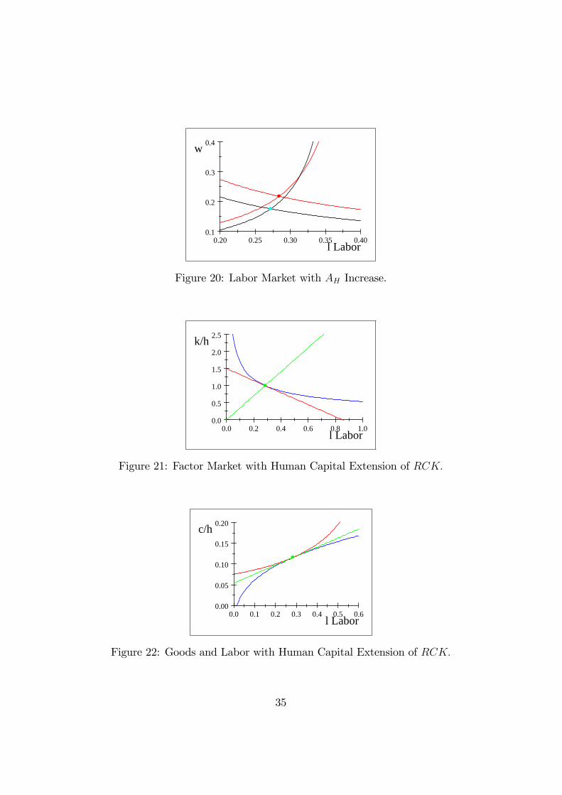
7.3 Output, Input General Equilibrium

The production possibility curve representation as well as the isoquant andisocost graphs follow through with human capital and endogenous growth.Again foregoing the equations, which follow in a fashion as described for theRCK model, Figures 21 and 22 present these graphs for the same examplecalibration and with normalization by ht:

34

0.20 0.25 0.30 0.35 0.400.1

0.2

0.3

0.4

l Labor

w

Figure 20: Labor Market with AH Increase.

0.0 0.2 0.4 0.6 0.8 1.00.0

0.5

1.0

1.5

2.0

2.5

l Labor

k/h

Figure 21: Factor Market with Human Capital Extension of RCK:

0.0 0.1 0.2 0.3 0.4 0.5 0.60.00

0.05

0.10

0.15

0.20

l Labor

c/h

Figure 22: Goods and Labor with Human Capital Extension of RCK:

35

8 Quali�cation and Conclusion

The most easy criticism of the approach here is that BGP equilibrium doesnot occur over the course of a business cycle and so cannot be used to ex-plain business cycles. Is this a fair criticism that can be used to argue thatAS � AD cannot be done in the dynamic recursive RCK model? I do notthink so. Economies are constantly being shocked and tending back towardstheir new equilibrium. Transition dynamics can be the most important storyin some cases. But over the business cycle can we really say that the econ-omy over some 4 or more years in an upturn, and sometimes as long in adownturn (although usually shorter) really have nothing to do with the equi-librium as in the stationary state? Consider that the shock processes in theRBC model is always with a persistence parameter near 0:95 whereas 1:0 isthe persistence parameter for a comparative static change as in the determin-istic analysis here. It is not so di¤erent, and "medium term" business cycleanalysis as in Comin and Gertler (2006) uses band-pass �lters that includethe low frequency. Given the ability to teach textbook style business cycleand growth with key RBC comparative statics changes using AS � AD, aspresented in this paper, it would seem to over-ride heuristic arguments thatwe cannot describe macroeconomic phenomena without transition dynamics.The paper shows that the AS �AD can be solved in the RCK dynamic

model by deriving the intratemporal and intertemporal equilibrium margins,�nding the closed-form solution for the capital stock, and graphing the supplyand demand in terms of the relative price of goods to leisure 1=w and outputy: The supply and demand are functions of the "state" variable, the capitalstock k; which is given (or shall we say "known") in equilibrium as of anygiven time t: Changes in goods and time endowments through changes ingoods productivity AG and time for work and leisure T can be used to showa business cycle, along with "Solow-plus" growth-trend stylistic facts. Goingbeyond undergraduates, human capital can be introduced with the result thatthe growth rate is endogenous. Changing human capital sectoral productivityAH causes an endogenous change in time for work and leisure T; such thata similar but perhaps more fundamental explanation of business cycle andSolow-plus growth facts result.The aim is to reinvigorate macroeconomics teaching so that the vast

36

chasm between graduate and undergraduate study is seamlessly bridged.Neoclassical AS � AD is a way to do this. Certainly it can be extended tohave any degree of price rigidity, monopoly power, or other Neo-Keynesianelements that one thinks should be there, with examples of �xed prices givenin Gillman (2011).The gradual evolution of macroeconomic thought has brought us from

the conceptions of aggregate demand in Keynes and in Samuelson�s (1951)Keynesian cross to where we have found ourselves today, rooted in an eclecticAS�AD static theory. Colander (1995) rightly points out the mix does notadd up to internal consistency. Rather than righting the analysis throughthe Keynesian side as he suggested might be done, here I have righted theanalysis through the Marshallian classical theory, something Keynes (1930)himself also explicitly set out to accomplish. But instead of de�ning pro�t asinvestment minus savings as did Keynes, I have followed Keynes�s brilliantstudent Ramsey (1928). Using a case of his exact model, AS �AD analysisfrom a Marshallian foundation is presented with zero BGP growth. Exten-sion to exogenous growth follows directly. Comparative statics describing abusiness cycle then become possible using Beckerian (1965) insights on timeendowment. Adding one more sector, human capital, and the Uzawa (1965)-Lucas (1988) extension of RCK also emerges in AS�AD terms. The storyof cycles and growth trends becomes enhanced by using changes only in thetwo sectoral productivitiesIt may appear surprising that this RCK analysis with AS � AD seems

not to have been presented before. For example Obstfeld and Rogo¤�s (1996)beautiful methodologically consistent development of macroeconomics couldhave had it embedded. Perhaps the early and ongoing controversy on con-sumption demand theory in terms of Friedman�s (1957) permanent incomehypothesis versus the consumption function in Samuelson (1951) has kept theconsumption demand within RCK under wraps and unexploited for derivingAD in the classical dynamic model. Such speculation on economic historygoes beyond the scope of this paper.Similarly the question of why endogenous growth of Uzawa-Lucas has

not become more mainstream remains a puzzle. The roots of disregardingit certainly start as far back as Cass (1965), who in a footnote commentsdirectly about Uzawa�s approach that he does not incorporate production of

37

investment in a separate sector since "no further insight is gained" (footnote2, p. 233). Certainly the success of Solow�s (1956) growth facts and Kydlandand Prescott�s (1982) RBC facts may indicate that further delving is un-necessary. However the bene�ts of human capital investment, the resultingnature of endogenous growth, and its potential enhancement of the RCKAS�AD analysis have been suggested in this paper as being of fundamentalinterest for students of macroeconomics.11

ReferencesAguiar, Mark and Hurst, Erik, 2009, "A Summary of Trends in American Time Allo-

cation: 1965�2005", Social Indicators Research, 93: 57�64.

Becker, Gary S., 1965, "A Theory of the Allocation of Time," The Economic Journal,

75(299): 493-517, September.

Benhabib, Jess and Rogerson, Richard and Wright, Randall, 1991. "Homework in

Macroeconomics: Household Production and Aggregate Fluctuations," Journal of Political

Economy, vol. 99(6), pages 1166-87, December.

Cass, David, 1965, "Optimum Growth in an Aggregative Model of Capital Accumu-

lation", Review of Economic Studies, 37 (3): 233�240, July.

Colander, David, 1995. "The Stories We Tell: A Reconsideration of AS/AD Analysis,"

Journal of Economic Perspectives, vol. 9(3), pages 169-88, Summer.

Comin, D and M. Gertler (2006), "Medium-term Business Cycles, American Economic

Review, 96, 3, 523-551.

Dang, Jing and Gillman, Max and Kejak, Michal, 2011. "Real Business Cycles with

a Human Capital Investment Sector and Endogenous Growth: Persistence, Volatility and

Labor Puzzles," Cardi¤ Economics Working Papers E2011/8.

Dellas, Harris and Koubi, Vally, 2003. "Business cycles and schooling," European

Journal of Political Economy, vol. 19(4), pages 843-859, November.

den Haan, Wouter J. & Sumner, Steven W., 2004. "The comovement between real

activity and prices in the G7," European Economic Review, 48(6, December): 1333-1347,

December.

Milton Friedman, 1957. "A Theory of the Consumption Function," NBER Books,

National Bureau of Economic Research, Inc.

11In a stochastic setting, Dang et al. (2011) suggest a solution to the fundamentalRBC consumption-output, growth persistence, and labor puzzles through a two-sectorendogenous growth model with an economy-wide shock to the productivity of both goodsand human capital sectors.

38

Gillman, Max, 2002. "Keynes�s Treatise : aggregate price theory for modern analy-

sis?," European Journal of the History of Economic Thought, vol. 9(3), pages 430-451.

Gillman, Max, 2011, Advanced Modern Macroeconomics, Pearson Financial-Times.

Gomme, Paul and Rupert, Peter, 2007. "Theory, measurement and calibration of

macroeconomic models," Journal of Monetary Economics, 54(2), pp. 460-497, March.

Greenwood, Jeremy and Hercowitz, Zvi, 1991. "The Allocation of Capital and Time

over the Business Cycle," Journal of Political Economy, 99(6), pp. 1188-1214, December.

Hansen, Gary D., 1985. "Indivisible labor and the business cycle," Journal of Mone-

tary Economics, vol. 16(3), pages 309-327, November.

Harberger, Arnold C. "A Vision of the Growth Process." American Economic Review,

1998, 88(1), pp. 1-32.

Keynes, John Maynard, 1923, A Tract on Monetary Reform, Macmillan and Co.,

Limited, London.

Keynes, John Maynard, 1930, A Treatise on Money, Macmillan and Co., Limited,

London.

Keynes, John Maynard, 1936, The General Theory of Employment, Interest and

Money, Macmillan and Cambridge University Press.

Koopmans, T. C., 1965, "On the Concept of Optimal Economic Growth", in The

Econometric Approach to Development Planning, Pontif. Acad. Sc. Scripta Varia 28, pp.

225-300.

Kydland, Finn E and Prescott, Edward C, 1982. "Time to Build and Aggregate

Fluctuations," Econometrica, vol. 50(6), pages 1345-70, November.

Lucas, Robert Jr., 1988. "On the mechanics of economic development," Journal of

Monetary Economics, vol. 22(1), pages 3-42, July

Obstfeld, Maurice and Kenneth Rogo¤, 1996, Foundations of International Macroeco-

nomics, The MIT Press, Cambridge, Massachusetts.

Ramsey F.P., 1928, "A Mathematical Theory of Saving," Economic Journal, Vol. 38,

No 152, pp. 543-559.

Rogerson, Richard, 1988. "Indivisible labor, lotteries and equilibrium," Journal of

Monetary Economics, vol. 21(1), pages 3-16, January.

Samuelson, Paul A., 1951, Economics: An Introductory Analysis, Second Edition,

McGraw-Hill Publishing Company Ltd, London.

Solow, Robert, 1956, "A Contribution to the Theory of Economic Growth," The Quar-

terly Journal of Economics, Vol. 70, No. 1, pp. 65-94, February.

39

Stokey, Nancy, Robert Lucas and Edward Prescott, 1989, Recursive Methods in Eco-

nomic Dynamics, Harvard University Press.

Uzawa,.Hirofumi, 1965, "Optimal Technical Change in An Aggregative Model of

Economic Growth", International Economic Review, Vol. 6, No. 1., pp. 18-31, January.

Varian, Hal R., 1978, Microeconomic Analysis, W. W. Norton & Company Inc., New

York.

40