As part of the Utility Rate Design Initiative, the ...

As part of the Utility Rate Design Initiative, the Alliance to Save Energy executed two technical

analyses and a review of literature. The first analysis investigated OpenEI’s U.S. Utility Rate

Database, an open-source utility tariff database, while the second analyzed the Energy Information

Administration’s Form 861 data. Additionally, the Alliance reviewed approximately 35 whitepapers

and technical documents that helped inform and shape its position on rate design.

This narrative accompanies and enhances the presentation materials from the May 12, 2016 kickoff

meeting. Both technical analyses are presented with additional background on process and results,

and a summary of selected whitepapers expands on the presentation's high level overview. Two

appendices are included, the first containing the ACEEE Scorecard-based state rankings that were

used in the two analyses, and the second containing a list of sources that were reviewed as part of

this phase of the initiative.

~ 2 ~

Acronyms ...................................................................................................................................................... 3

OpenEI U.S. Utility Rate Database Analysis ................................................................................................ 4

Fixed Charges ........................................................................................................................................... 6

Seasonal/Monthly Demand Charges ................................................................................................... 14

Time of Use Demand Charges .............................................................................................................. 20

Seasonal/Monthly Energy Charge ....................................................................................................... 22

Time of Use Energy Charge .................................................................................................................. 26

Concluding Thoughts ............................................................................................................................ 29

EIA Form 861 Analysis .............................................................................................................................. 30

Macro Trends in the Electric Industry .................................................................................................. 31

Advanced Metering Infrastructure Deployment .................................................................................. 35

Utility Performance by ACEEE Scorecard Quintile Ranking ................................................................ 39

Policy Impacts on Energy Efficiency Savings ....................................................................................... 43

Residential EE Savings Cross-Analysis with OpenEI Database .......................................................... 45

Concluding Thoughts ............................................................................................................................ 46

Review of Literature .................................................................................................................................. 47

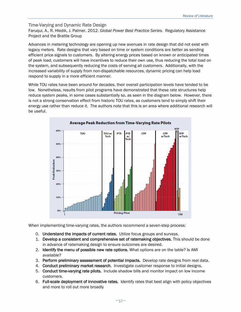
Smart Rate Design for a Smart Future ................................................................................................ 48

Designing a New Utility Business Model? Better Understand the Traditional One First .................. 49

Moving Toward Value in Utility Compensation. Part One – Revenue and Profit. .............................. 49

Electric Industry Structure and Regulatory Responses in a High Distributed Energy Resources

Future .................................................................................................................................................... 51

Distribution Systems in a High Distributed Energy Resources Future: Planning, Market Design,

Operation and Oversight ....................................................................................................................... 52

Performance-Based Regulation in a High Distributed Energy Resources Future ............................. 53

Pathway to a 21st Century Electric Utility ............................................................................................. 54

Rate Design for the Distribution Edge: Electricity Pricing for a Distributed Resource Future .......... 55

Electric Utility Residential Customer Charges and Minimum Bills: Alternative Approaches for

Recovering Basic Distribution Costs .................................................................................................... 56

Time-Varying and Dynamic Rate Design .............................................................................................. 57

Appendix A – ACEEE Ranking and Quintile .............................................................................................. 58

Appendix B – List of Sources.................................................................................................................... 59

~ 3 ~

AMI: Advanced Metering Infrastructure

DER: Distributed Energy Resources

DG: Distributed Generation

CPP: Critical Peak Pricing

DP: Dynamic Pricing

DR: Demand Response

DSM: Demand Side Management

EE: Energy Efficiency

EERS: Energy Efficiency Resource Standard

EM&V: Evaluation, Measurement, and Verification

LRAM: Lost Revenue Adjustment Mechanism

PIM: Performance Incentive Mechanism

RDI: Rate Design Initiative

RPS: Renewable Portfolio Standard

TOU: Time of Use

TVR: Time-Varying Rates (includes TOU and DPP)

VI: Vertically Integrated

~ 4 ~

The first Utility Rate Design Initiative (RDI) technical analysis investigated the OpenEI U.S. Utility Rate

Database. This database, hosted by non-profit Open Energy Information, contains detailed

information about utility rate tariffs. Users can search by zip code, utility name, sector (e.g.

residential, commercial, industrial, and lighting) and effective date. The database contains almost

40,000 tariffs as of May 2016 (including 30,500 active tariffs from over 2,800 utilities), and

additional tariffs are added or updated frequently.

For its analysis, the Alliance made two decisions to limit the scope of the dataset. First, it excluded

lighting tariffs from detailed analysis. While lighting tariffs are an interesting aspect to rate design,

they are sufficiently distinct in their characteristics from traditional residential, commercial, and

industrial tariffs to merit their exclusion as part of this effort. Second, it focused primarily on

Municipal, Cooperative, and IOU tariffs. This excluded tariffs from political subdivisions (i.e. irrigation

districts), state, and federal tariffs. After applying these two filters, nearly 75% or 23,000 tariffs

remained of the original dataset, shown in green below.

Municipal Cooperative IOU Political

Subdivision

State Federal Retail Power

Marketer

Grand

Total

Count of Utilities 1,786 757 169 95 7 4 2 2,820

Tariffs by Sector

Commercial 6,246 3,931 2,002 739 83 77 13,078

Industrial 2,447 1,442 788 267 17 10 4,971

Residential 3,254 1,836 881 224 25 2 3 6,225

Lighting 3,101 2,434 310 405 14 5 6,269

Grand Total 15,048 9,643 3,981 1,635 139 94 3 30,543

One of the limitations of the tariff database is that it does not include the level of participation of a

particular tariff. While this precludes the ability to produce weighted averages of certain rate

characteristics, the database is still amenable to the analysis of prevalence of a given characteristic.

Five major tariff charges were analyzed. These include:

Fixed (i.e. customer) charges Charges that appear on every bill every billing cycle, regardless of energy use or demand levels.

Seasonal/monthly demand charges Charges that are based on the highest demand of a customer over a billing period, typically

measured in $/kW (but sometimes in $/kVA or $/HP). Seasonal demand charges may include a

different demand rate for summer and winter months, while monthly tariffs might vary by month.

Additionally, demand tariffs may have different tiers (i.e. one up to 100 kW and another for over 100

kW) with correspondingly different rate levels.

Time of use demand charges Charges that are based on the highest demand of a customer over a shorter time frame, analogous

to the more common time of use energy rates. In these rates, customers might face one rate during

weekday peak hours and another during weekend or off-peak hours. There may also be a seasonal

component to the rate levels.

Seasonal/monthly energy charges Charges that are based on a $/kWh rate. As with seasonal or monthly demand charges, these rates

may vary season-to-season or month-to-month, and may have different tiers with different prices.

http://en.openei.org/apps/USURDB/

http://en.openei.org/wiki/Main_Page

OpenEI U.S. Utility Rate Database Analysis

~ 5 ~

Time of use (TOU) energy charges Charges that are based on a $/kWh rate that vary based on what time of day or week the energy is

consumed. A typical rate structure might include on-peak, intermediate, and off-peak period rates.

TOU tariffs can also include a seasonal aspect or a tiered structure.

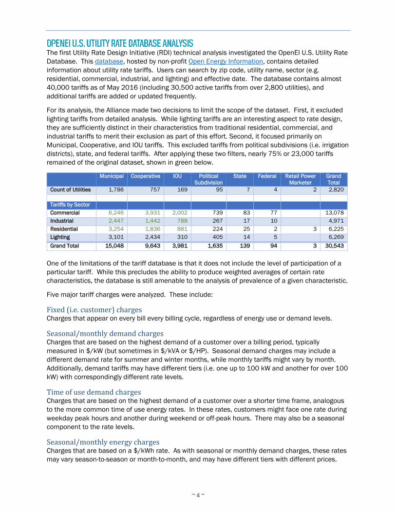
Tariffs were analyzed through three main groupings.

Grouping Details

Utility type Tariffs grouped by municipal, cooperative, and IOU utilities. Other

ownership types (political subdivision, federal, state, and retail power

marker) were not analyzed in detail.

Sector Tariffs grouped by Commercial, Industrial, and Residential. Lighting tariffs

were not analyzed in detail.

ACEEE Quintile ranking ACEEE Quintile rankings were calculated from the cardinal rank of the

average rank of each state’s 2011-2015 scorecard. Rankings are

included in Appendix A.

By analyzing trends across sectors and across utility types, and comparing rate characteristics to

ACEEE rankings, the Alliance was able to glean some insights from the dataset that might help

inform RDI ratemaking principles. Each characteristic was analyzed to determine how often it was

found in the tariffs of each utility type and sector. In the charts that follow, the darker shading

indicates the percentage of the tariffs with that characteristic. For fixed charges and demand

charges, histograms showing the relative scale of the charges were calculated for each

combination.1 Additional analyses on inclining and declining block structures and on TOU rates are

found in their respective sections.

1 Histograms for energy charges were not calculated as they tend to be driven more by an individual utility’s

fuel costs (for vertically integrated utilities) and/or the residual revenue requirement after fixed and demand

charges are taken into account.


~ 6 ~

Fixed Charges

Fixed charges are a staple of tariffs found in the OpenEI database. For each sector/utility ownership

combination, almost 85% of tariffs included some sort of fixed charge.2 For IOUs, the figure exceeds

90% across all sectors.

For IOU residential tariffs, 32 states had a fixed charge in 100% of their database tariffs. For the

other 18 states, most had fewer than 10% of tariffs without a fixed charge. Notable exceptions

include California, where 27% of residential tariffs lacked a fixed charge, and Alaska, where nearly

60% did not have a fixed charge.

When one looks at the distribution of fixed charges, some observations can be made based on the

sector and ownership structure of the utility.

2 In each of the stacked vertical bar charts, the percentage of tariffs with the characteristics is shaded darker,

while the balance without the characteristic is shaded lighter.

0%

10%

20%

30%

40%

50%

60%

70%

80%

90%

100%

Com Ind Res Com Ind Res Com Ind Res

Tariffs with Fixed Charges

Municipal Cooperative IOU

0%

10%

20%

30%

40%

50%

60%

70%

NY IA MN MO NC OR OH MI NV LA ME AZ CA VT ID AK

% o

f Ta

riff

s w

ith

ou

t a

Fixe

d c

har

ge

Residential IOU Tariffs without a Fixed Charge


~ 7 ~

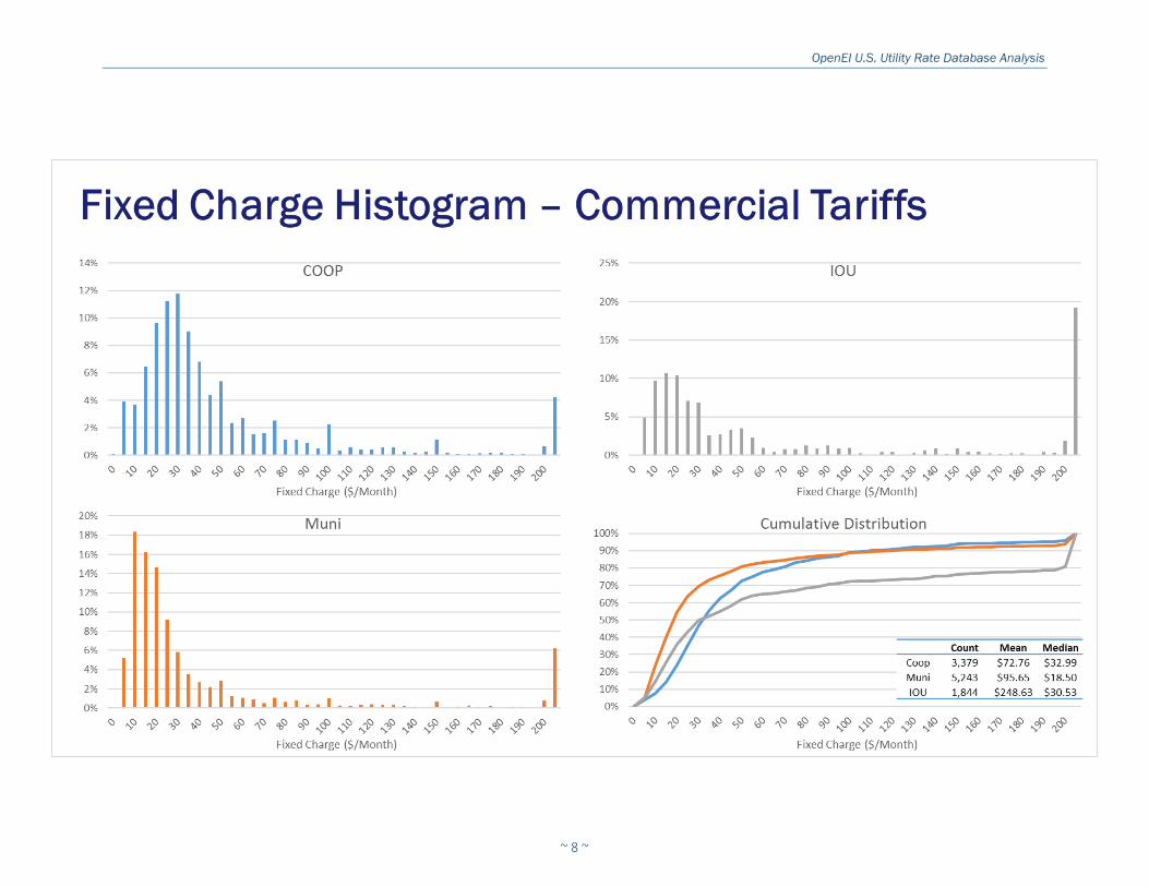
Within the commercial sector, there was a reasonable amount of variation in the fixed charge

distribution. Generally, municipal utilities had the lowest fixed charges, with peaks occurring at

$10/month and 70% having a charge of $30/month or less. On the other hand, the most common

fixed charge for IOUs (nearly 20% of tariffs) exceeded $200/month. Cooperatives were somewhat in

the middle of the two distributions, with more tariffs clustered around $30/month, but with a

reasonable proportion over $200/month. These differences also emerge when looking at the mean

and median fixed charge. IOUs have by far the highest average, driven by the large quantity of tariffs

with high fixed charges. But the median commercial tariff for IOUs is actually slightly lower than the

median commercial tariff for coops.

Industrial tariffs tell a different story. Here, the distribution of the coop and municipal utilities is

nearly identical, but the IOU is starkly different. As with the commercial sector, IOU fixed charges in

the industrial sector are skewed toward the high end of the spectrum. In this distribution, roughly a

third of all tariffs exceeded $800/month, while only 12% of coop and muni industrial tariffs were

above this level. Again, the mean and median reflect this story with the average industrial IOU tariff

fixed charge set 7 and 9 times higher than the muni and coop, respectively.

Curiously, the residential tariffs tell a similar story to the industrial but with a change in the actors. In

this sector, the muni and IOU customers are virtually indistinguishable, with the coops acting as the

outlier. Coop fixed charges are higher and their distribution is broader, with a larger proportion of

high outlier fixed charges. One possible reason for this is that many rural coops classify agricultural

customers under their residential tariff, skewing their dataset with “commercial-like” tariffs.

Nonetheless, the median cooperative residential customer (who is insulated from the upward skew

of the mean customer) pays $21.50/month in fixed charges, as compared to $9.00 and $9.57 per

month for muni and IOU residential customers, respectively. By the time the IOU distribution hits

$21.50 per month, 93% of ratepayers will have lower fixed charges.


~ 8 ~


~ 9 ~


~ 10 ~


~ 11 ~

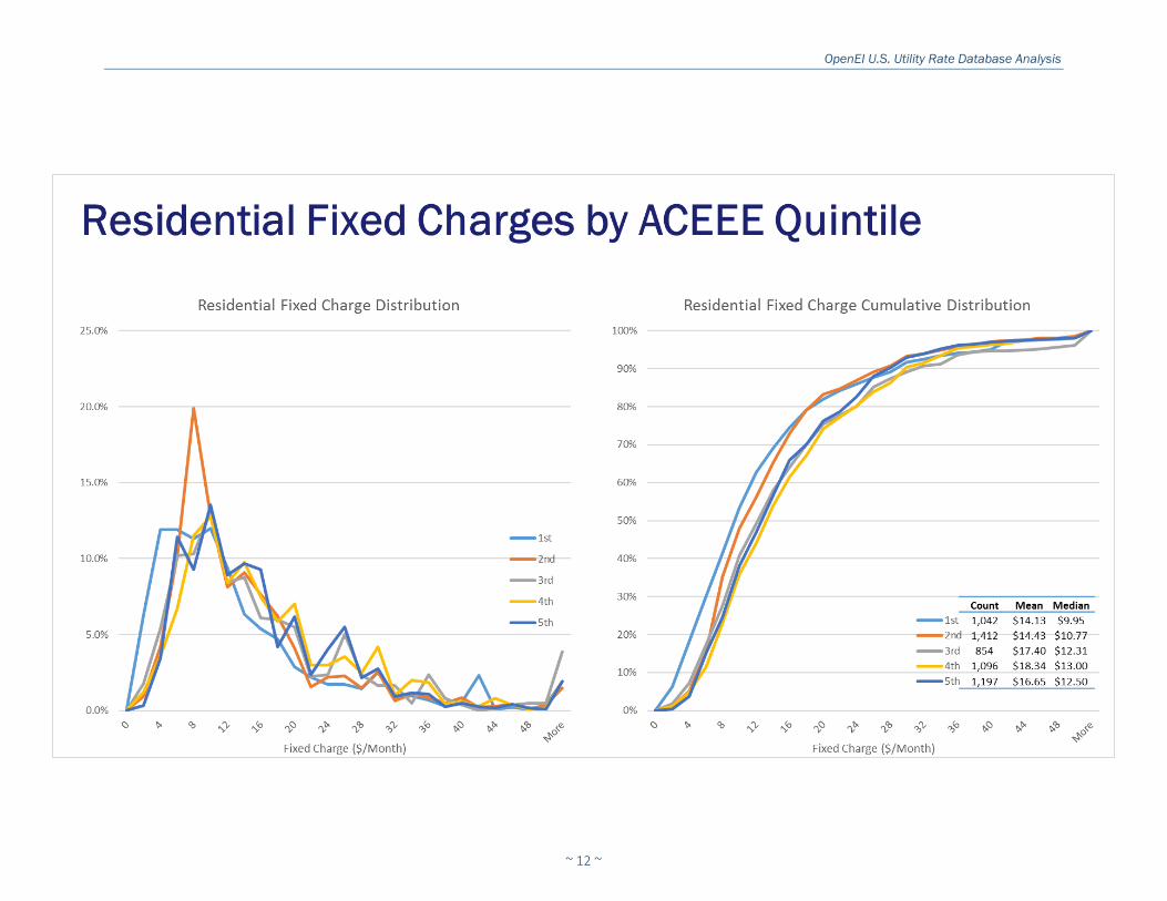
The last set of fixed charge analysis compares the prevalence of fixed charge levels to ACEEE

Quintile performance. In these charts, each sector was analyzed by state across utility ownership

structures, and a common distribution based on ACEEE Quintile was developed. While this

methodology does combine several factors that might influence utility energy efficiency performance,

some patterns do emerge from the data.

For residential customers, energy efficiency performance (as measured by the proxy of ACEEE

Quintile ranking) is correlated with lower fixed charges. The mean fixed charge for the top two

quintiles was $3.20 lower than the bottom three quintiles, a reduction of almost 20%. The lower

fixed charges are maintained throughout the cumulative distribution until the tariffs begin to

converge around the 90th percentile.

For commercial customers, the relationship is not as strong across the spectrum. In fact, the

cumulative distribution for the 2nd and 5th quintiles have the lowest fixed charges, with the 1st, 3rd,

and 4th more closely distributed on the high end of the fixed charge spectrum. That said, the data for

the lower half of the distribution (i.e. customers with lower than median fixed charges) show 1st and

2nd quintile states with lower fixed charges than the other three quintile states.


~ 12 ~


~ 13 ~


~ 14 ~

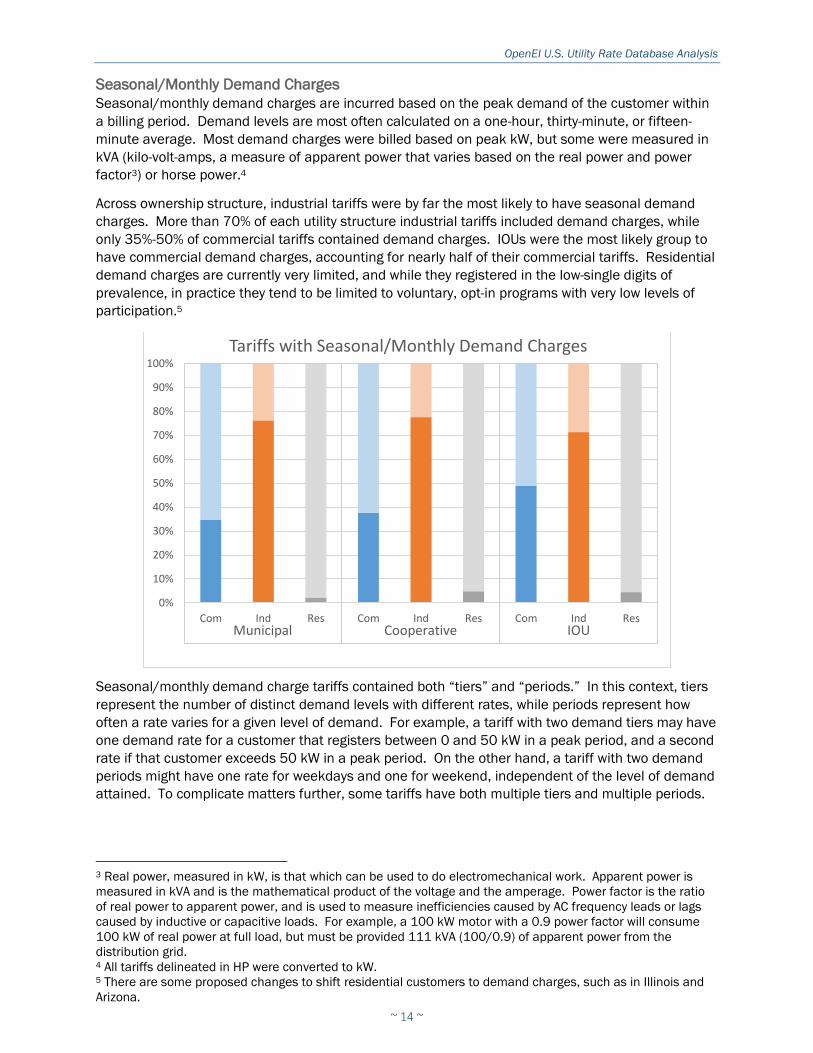
Seasonal/Monthly Demand Charges

Seasonal/monthly demand charges are incurred based on the peak demand of the customer within

a billing period. Demand levels are most often calculated on a one-hour, thirty-minute, or fifteen-

minute average. Most demand charges were billed based on peak kW, but some were measured in

kVA (kilo-volt-amps, a measure of apparent power that varies based on the real power and power

factor3) or horse power.4

Across ownership structure, industrial tariffs were by far the most likely to have seasonal demand

charges. More than 70% of each utility structure industrial tariffs included demand charges, while

only 35%-50% of commercial tariffs contained demand charges. IOUs were the most likely group to

have commercial demand charges, accounting for nearly half of their commercial tariffs. Residential

demand charges are currently very limited, and while they registered in the low-single digits of

prevalence, in practice they tend to be limited to voluntary, opt-in programs with very low levels of

participation.5

Seasonal/monthly demand charge tariffs contained both “tiers” and “periods.” In this context, tiers

represent the number of distinct demand levels with different rates, while periods represent how

often a rate varies for a given level of demand. For example, a tariff with two demand tiers may have

one demand rate for a customer that registers between 0 and 50 kW in a peak period, and a second

rate if that customer exceeds 50 kW in a peak period. On the other hand, a tariff with two demand

periods might have one rate for weekdays and one for weekend, independent of the level of demand

attained. To complicate matters further, some tariffs have both multiple tiers and multiple periods.

3 Real power, measured in kW, is that which can be used to do electromechanical work. Apparent power is

measured in kVA and is the mathematical product of the voltage and the amperage. Power factor is the ratio

of real power to apparent power, and is used to measure inefficiencies caused by AC frequency leads or lags

caused by inductive or capacitive loads. For example, a 100 kW motor with a 0.9 power factor will consume

100 kW of real power at full load, but must be provided 111 kVA (100/0.9) of apparent power from the

distribution grid. 4 All tariffs delineated in HP were converted to kW. 5 There are some proposed changes to shift residential customers to demand charges, such as in Illinois and

Arizona.

0%

10%

20%

30%

40%

50%

60%

70%

80%

90%

100%


Tariffs with Seasonal/Monthly Demand Charges



~ 15 ~


~ 16 ~

Tariffs with a single annual demand charge were analyzed in more detail. As seen above, a large

percentage of tariffs with demand charges billed a constant price per kW throughout the year

(indicated by the “1” entry under each utility type in the right chart above.) Unlike the fixed charge

histograms, there was not a substantial variation between the utility types in a given sector.

In the commercial sector, the distribution of demand levels was fairly similar. Median rates were

slightly lower for coops ($6.86/kW) than for munis ($7.68/kW) and IOUs ($7.23/kW), but the

cumulative distribution was not driven by an unusually high level of outliers.

Industrial tariffs had a bit more variation, with IOUs generally skewing towards the low end of the

price distribution. Municipal utilities had a large peak in the $2/kW range (with nearly 20% of

industrial tariffs in that bucket), but were otherwise fairly evenly distributed. Coops peaked around

$7/kW.

Interestingly, the median and mean demand charges were about 25% and 22% higher, respectively,

for IOU commercial customers than for IOU industrial customers.

Residential annual demand charges are not very common, with only 128 in the active tariff dataset.

But for the small sample, the levels and distribution were relatively consistent across the utility

types. Average residential demand rates were in between commercial and industrial levels.


~ 17 ~


~ 18 ~


~ 19 ~


~ 20 ~

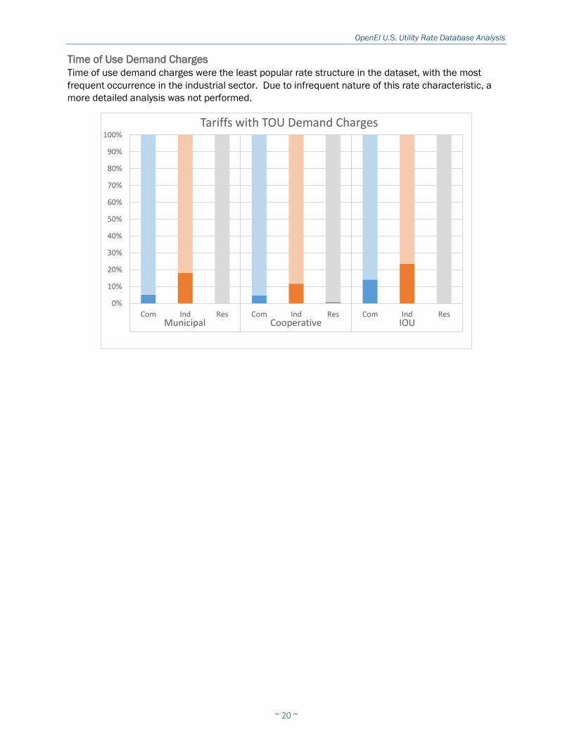
Time of Use Demand Charges

Time of use demand charges were the least popular rate structure in the dataset, with the most

frequent occurrence in the industrial sector. Due to infrequent nature of this rate characteristic, a

more detailed analysis was not performed.

0%

10%

20%

30%

40%

50%

60%

70%

80%

90%

100%


Tariffs with TOU Demand Charges



~ 21 ~


~ 22 ~

Seasonal/Monthly Energy Charge

While TOU demand charges are the least common, tariffs with seasonal/monthly energy charges are

by far the most common. More than 95% of all sector/ownership combos (with the exception of

Industrial/IOU) contained these rates. This is to be expected, as a kWh-based energy charge is the

core volumetric rate that most mass market consumers associate with their electricity bill.

Of the few tariffs that did not include an energy charge, most were for specialty situations such as

back-up power or unmetered rates. And while the lighting sector was not a focus of this analysis,

roughly 85-95% of lighting tariffs did not have an energy charge.

There are more instances of multi-tier and multi-period energy charges than demand charges,

although solid majorities of tariffs still consist of one year-round tier. The most obvious exception is

in IOUs, where more than 50% of tariffs across sectors have at least 2 periods (with the most

common in the form of a summer/winter rate structure).

A large minority of energy tariffs have a block structure. That is, energy prices for the first block of

kWh consumed vary from prices for the second (or third or fourth) block consumed. These blocks

vary by their width (i.e. how many kWh are in a block) and relative size (how much the price changes

between blocks). A number of tariffs have a “free first” structure, where the first block of kWh are

free (or presumably included in a fixed charge), and customers are only charged after consuming a

certain quantity of electricity.

Of tariffs with a block structure, 83% were declining or “free first” declining, and only 14.5% were

inclining or “free first” inclining (the balance had “free first” then flat structures). In the commercial

and industrial sectors, declining block structurers were even more common, comprising roughly 95%

of tariffs with a block structure. Residential tariffs had a less unbalanced split between declining

and inclining block structures, but two-thirds of residential block tariffs were declining. Additionally,

IOUs were more likely to have an inclining block structure than either cooperatives or municipal

utilities.

For those tariffs with increases or decreases in the second block pricing, the change in pricing varied

considerably. While some tariffs had relatively small (10%-20%) changes between tiers, others

changed much more dramatically. Of the residential tariffs with inclining block structures, nearly

0%

10%

20%

30%

40%

50%

60%

70%

80%

90%

100%


Tariffs with Seasonal/Monthly Energy Charges



~ 23 ~

40% had at least a 25% increase in price between tiers, and nearly 25% had price increases in

excess of 50%, and about 10% saw prices more than double, with increases over 100%.

From an energy efficiency perspective, the prevalence of declining block structures is not ideal. By

pricing the marginal kWh lower than the initial kWh, customers have less incentive to reduce their

energy use. One potential explanation is that fixed customer charges might be higher in tariffs with

declining block structures, but the data did not bear that out. While residential IOU tariffs with

declining block structures did have a slightly higher median fixed charge, it was not substantially

different than those with including block structures. An in contrast to this theory, both the median

municipal and cooperative residential fixed charge were actually higher in the inclining block

structures than in the declining block structures.


~ 24 ~


~ 25 ~


~ 26 ~

Time of Use Energy Charge

Time of use (TOU) energy charges are relatively common in the tariff dataset. They occur most often

in the residential sector across utility types, and among IOU tariffs across sectors. Anecdotally, the

majority of TOU rates remain voluntary with an opt-in, and participation rates are not as high as the

existence of the tariffs might indicate. That is, even though 60% of IOUs offer a residential TOU tariff,

a substantially smaller percentage of customers are actually on those tariffs.6

TOU energy rates can also contain tiers and periods, leading to very complex rates.7 While most TOU

rates only have two periods (i.e. on-peak and off-peak), nearly 40% of IOU TOU tariffs have three or

more periods. A peak/intermediate/off-peak rate structure is rather common.

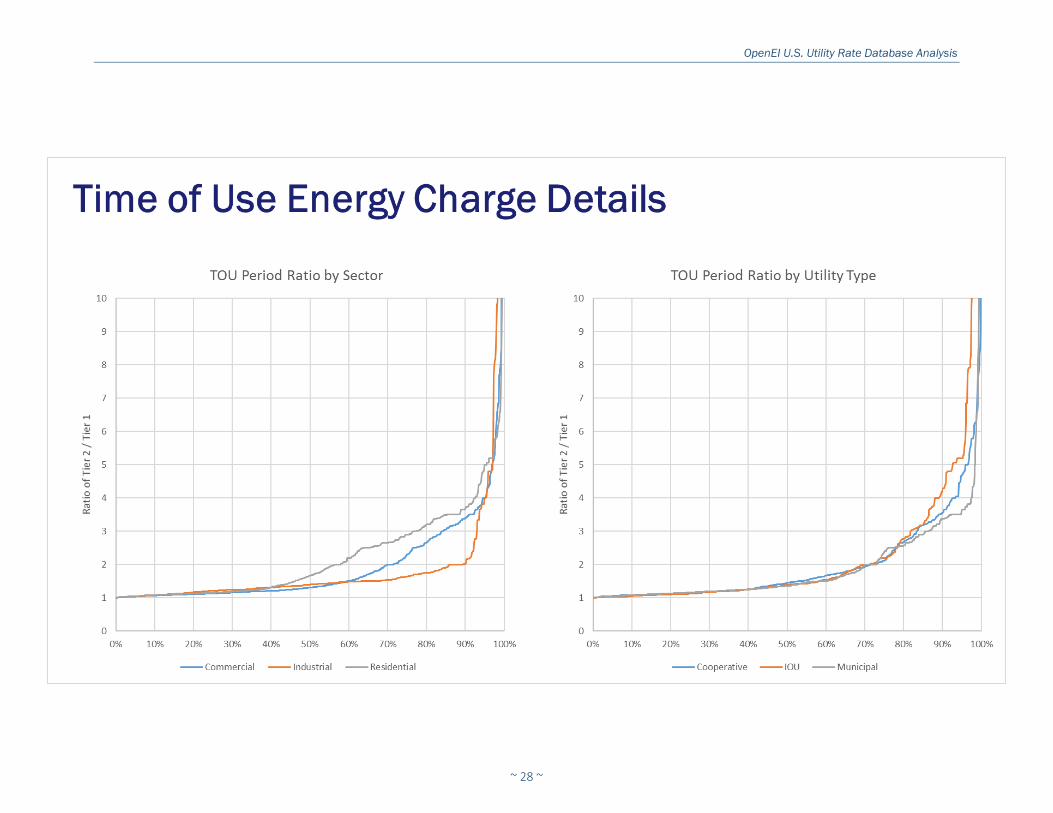
The relative cost of each period varies more between classes than it does between utility types. For

TOU tariffs with two periods and one tier, the ratio between residential peak and off-peak rates

began to separate from the commercial and industrial classes after the 40 percentile of the tariff’s

cumulative distribution, and stayed above of the other two sectors through the 95 percentile of the

distribution. About 40% of residential tariffs had a peak/off-peak ratio of 2 or more (i.e. peak energy

costing at least twice as much as off-peak energy), with about a quarter set at 3 or more.

Commercial tariffs also separated from industrial tariffs at about the 60 percentile mark, but

rejoined around the 95 percentile. Industrial customers maintained a very low ratio for the vast

majority of their distribution, only to increase sharply for the last 10% of tariffs.

6 As with demand charges, there is some movement in this area. Recent California rate settlements will move

residential customers to a mandatory TOU rate in 2019. 7 Some California rates included 4 tiers and 4 periods, with costs for energy use changing seasonally, weekly,

and hourly based on daily usage.

0%

10%

20%

30%

40%

50%

60%

70%

80%

90%

100%


Tariffs with TOU Energy Charges



~ 27 ~


~ 28 ~

~ 29 ~

Concluding Thoughts

Rate design must balance a number of considerations, and be wary of both intended and

unintended consequences. Good rate design allows a utility to recover its justified costs while

enabling policy makers to incent behavior that benefits utility customers and society writ large. Bad

rate design, on the other hand, may be punitive to a particular customer class or promote behavior

that does not advance either the utility’s bottom line or the value delivered to the customer.

In the OpenEI database, we see a huge variety of rate designs that have been implemented to

balance and address these issues. Our analysis was not intended to claim which utilities are doing

rate design correctly and which are not, but rather to see what, if any, trends emerge when analyzing

a broad cross-section of different rate-making approaches. We are able to draw a few conclusions

from this effort.

Broadly speaking and excluding outliers, IOUs are more likely than cooperative and municipal utilities

to have rate structures that recover more costs from mass-market consumers (i.e. residential and

commercial) through variable rates rather than through higher fixed charges. They are the most

likely to utilize seasonal and TOU energy rates as well. For their industrial customers, IOUs tend to

have higher fixed charges and lower demand rates than coops and munis. Finally, IOUs are the most

likely to utilize an inclining block structure and to have more complex TOU rates.

Cooperatives have the highest distribution of residential fixed charges of the three utility types, and

also the most likely to have the simplest one-tier, one-period energy rate structure. In other ways,

they appeared very similar to municipal utilities (implementation of seasonal demand charges, low

prevalence of TOU rates).

Rate design is as much a product of the regulatory environment as it is of the utility ownership

model. While a broad-based analysis of tariffs in the OpenEI database is instructive to see some of

these trends, state variations in policy tend to have an outsized impact on energy efficiency

performance. The second analytical effort in the RDI sought to further explore this issue.

~ 30 ~

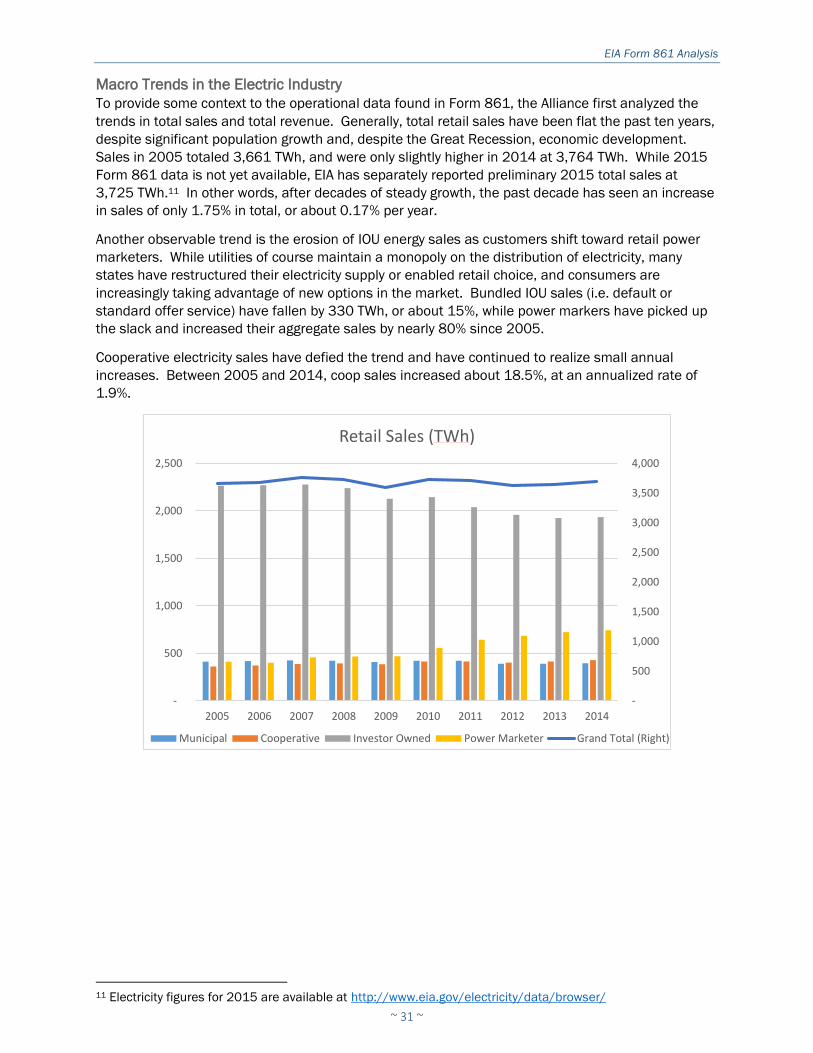
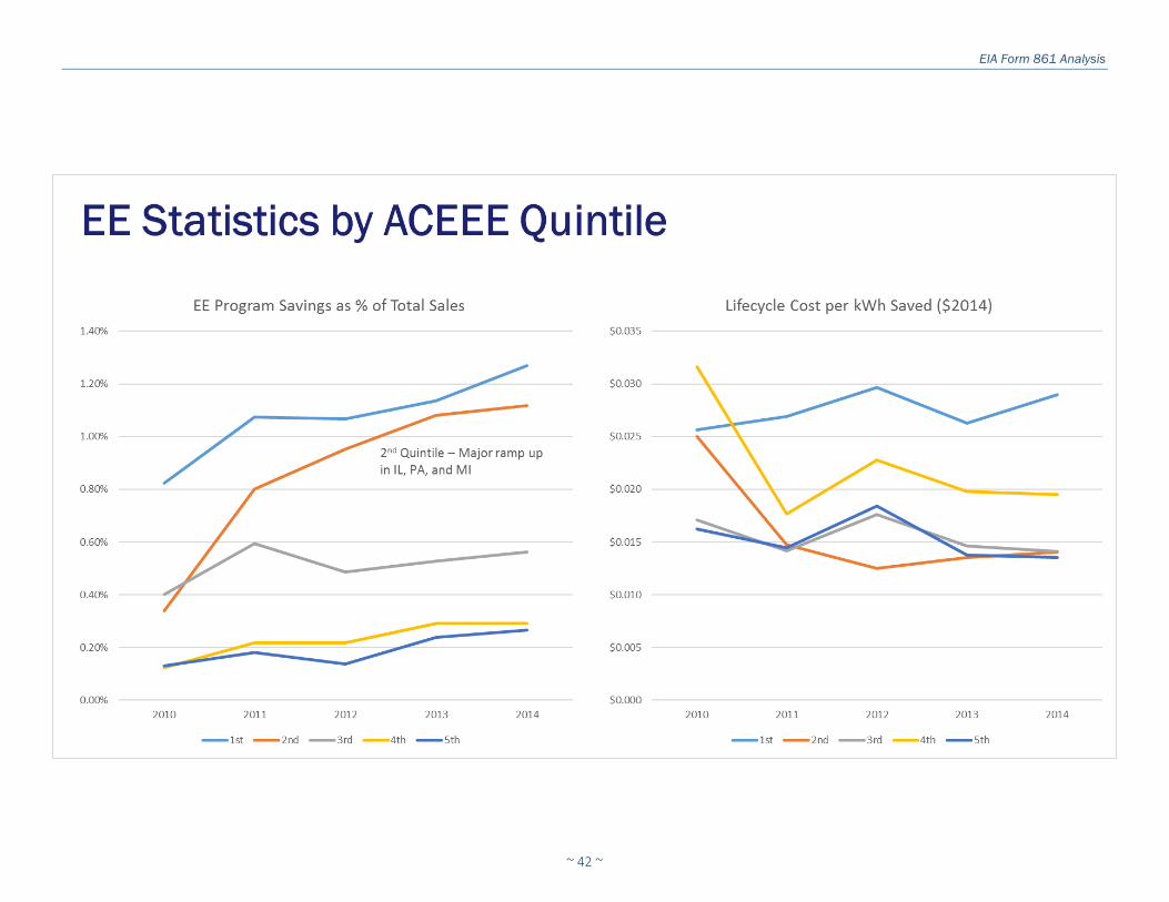
The second major analysis performed by the Alliance for the RDI analyzed the Energy Information

Administration’s (EIA) Form 861. Form 861, the Annual Electric Power Industry Report, contains

myriad details about the operational characteristics of electric utilities.8 While the file format and

data collected has evolved over the years, the data was substantially consistent enough to allow the

Alliance to combine ten years of data (2005-2014) into one dataset for analysis.9

Form 861 contains operational data on sales, revenues, and customer counts, broken down by

residential, commercial, industrial, and transportation sectors. The data also includes energy and

demand savings and spending on utility energy efficiency (EE) and demand response (DR) programs,

although some of the data collected in these areas changed through the years.10 Finally, other

information such as the existence of dynamic pricing and automated metering infrastructure is

included to varying degrees through the years.

While many utilities include EE program data directly, several states have third-party implementers

(such as NYSERDA and VEIC in New York and Vermont, respectively) that manage EE programs on

behalf of the state’s utilities. Fortunately, this data is also included in the forms, although it requires

that data on EE spending and savings in states with third-party implementers are analyzed at the

state level rather than the utility level.

In addition to the data found in EIA’s forms, the Alliance analyzed information from the Edison

Electric Institute (EEI), an electric IOU trade association, to gain some perspective on the macro

trends facing the electric industry. These two datasets were not merged, but insights into industry

capital investment helps inform the observations regarding utility revenues from electricity sales.

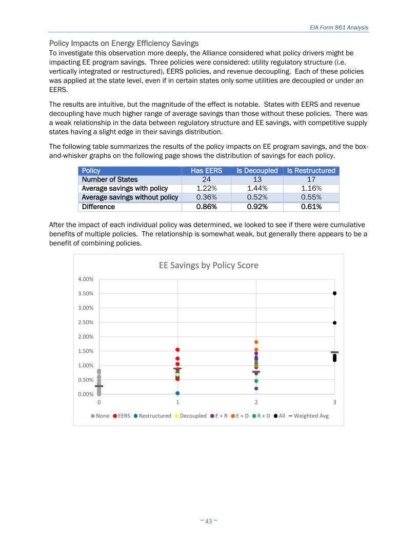
The Alliance incorporated additional policy considerations at the state level, including whether a

state was restructured or partially-restructured, whether the state had an energy efficiency resource

standard (EERS), whether revenue decoupling had been instituted, and what the state’s average

ACEEE Scorecard ranking was over the past five years.

As with the OpenEI analysis, the Alliance focused the Form 861 analysis on IOU, municipal, and

cooperative utilities, while adding additional analysis on retail and wholesale power marketers as

appropriate.

8 Form 861 data is available at https://www.eia.gov/electricity/data/eia861/ 9 EIA created a Short Form in 2012 that smaller utilities could fill out in lieu of the full Form 861. This data was

merged back into the main dataset on an element-by-element basis as appropriate. 10 The data is limited to utility-based programs and does not capture savings from ESCOs or other third-party

business-to-business programs.

https://www.eia.gov/electricity/data/eia861/

EIA Form 861 Analysis

~ 31 ~

Macro Trends in the Electric Industry

To provide some context to the operational data found in Form 861, the Alliance first analyzed the

trends in total sales and total revenue. Generally, total retail sales have been flat the past ten years,

despite significant population growth and, despite the Great Recession, economic development.

Sales in 2005 totaled 3,661 TWh, and were only slightly higher in 2014 at 3,764 TWh. While 2015

Form 861 data is not yet available, EIA has separately reported preliminary 2015 total sales at

3,725 TWh.11 In other words, after decades of steady growth, the past decade has seen an increase

in sales of only 1.75% in total, or about 0.17% per year.

Another observable trend is the erosion of IOU energy sales as customers shift toward retail power

marketers. While utilities of course maintain a monopoly on the distribution of electricity, many

states have restructured their electricity supply or enabled retail choice, and consumers are

increasingly taking advantage of new options in the market. Bundled IOU sales (i.e. default or

standard offer service) have fallen by 330 TWh, or about 15%, while power markers have picked up

the slack and increased their aggregate sales by nearly 80% since 2005.

Cooperative electricity sales have defied the trend and have continued to realize small annual

increases. Between 2005 and 2014, coop sales increased about 18.5%, at an annualized rate of

1.9%.

11 Electricity figures for 2015 are available at http://www.eia.gov/electricity/data/browser/

-

500

1,000

1,500

2,000

2,500

3,000

3,500

4,000

-

500

1,000

1,500

2,000

2,500

2005 2006 2007 2008 2009 2010 2011 2012 2013 2014

Retail Sales (TWh)

Municipal Cooperative Investor Owned Power Marketer Grand Total (Right)

http://www.eia.gov/electricity/data/browser/


~ 32 ~

Turning to total revenue,12 we see a somewhat different story for IOUs and power marketers.

Because IOUs continue to receive revenue for delivering competitive supply, they are somewhat

insulated from the reduction in their sales volumes shown earlier. This chart shows an incomplete

picture of their regulated profits, as certain categories such as fuel costs are passed through as

operational expenses on which utilities do not earn a return. Nonetheless, their total revenue in real

terms has fallen from a peak of $294b in 2008 to $260b in 2012, before rebounding slightly to

$272b in 2014. Total revenues for the entire electricity sector are down about 3% in real terms in

2015,13 so it would be expected for IOUs to see some drop in their 2015 revenue as well.

Power marketers, on the other hand, have seen substantial volatility in their revenues over the past

decade. Revenue peaked in 2008, with spikes in natural gas prices driving up the cost of electricity.

But even as power marketer sales grew over the subsequent years, electricity prices continued to

fall. Real revenue is down nearly 35% from $249b in 2008 to $165b in 2014, despite an increase

in sales volume of 60% over the same time period. The steep and continued fall of natural gas

prices have kept wholesale rates low, and the corresponding revenue figures reflect this.

As mentioned above, profits for vertically integrated and restructured IOUs come from different

sources. While both earn money on assets used to deliver power, restructured IOUs do not

(generally) earn a return on power plant assets. Data in Form 861 is collected for bundled revenue

(i.e. delivery plus energy for default or standard offer service) and for delivery-only revenue (revenue

from customers in restructured states who use competitive suppliers). Through some manipulation

of the data, we were able to extract the approximate revenues for both supply and distribution for

distribution-only IOUs operating in restructured markets.14

As seen below, revenue from vertically integrated utilities (blue columns) has grown in real terms

over the past decade, although most of that growth took place between 2005 and 2010, with

revenues flat between 2010 and 2014. On the other hand, total revenues from IOUs operating in

12 All revenue figures were converted to $2014 using the GDP deflator unless otherwise noted. 13 Supra note 11 14 Generally, a distribution and SOS rate (including distribution) were calculated for each utility/class

combination. The distribution rate was subtracted from the SOS rate to obtain a supply-only rate for the

bundled product. Finally, the rates were converted back into revenue by multiplying by sales volumes, and

distribution revenues were summed across distribution-only and bundled energy products.

$0

$50

$100

$150

$200

$250

$300

$350

2005 2006 2007 2008 2009 2010 2011 2012 2013 2014

Revenue from Sales ($2014b)

Investor Owned Power Marketer


~ 33 ~

restructured states (orange and grey columns) show that total revenues have fallen steeply since

2009, corresponding to the drop in electricity supply prices. But even this is not the whole story.

Because restructured utilities earn a return on their distribution assets, and bundled energy is

typically treated as an operational expense pass-through, the revenue associated with the underlying

distribution service is a more important financial metric. We see below that distribution revenue has

grown slightly in real terms in 8 of the past 10 years, resulting in a 10-year real CAGR of 1.02%.

$0

$20

$40

$60

$80

$100

$120

$140

2005 2006 2007 2008 2009 2010 2011 2012 2013 2014

IOU Total Revenue by Regulation ($2014b)

Vertically Integrated Distribution Energy (SOS)

$0

$10

$20

$30

$40

$50

$60

$70

$80

$90

$100

2005 2006 2007 2008 2009 2010 2011 2012 2013 2014

Restructured Utility Revenue ($2014b)

Distribution Energy (SOS)


~ 34 ~

Of course, these figures are aggregated across the entire utility industry, and individual utilities might

have seen higher or lower growth in their revenues. Nonetheless, from this data, it appears that the

entity whose revenues are most affected by the precipitous drop in natural gas prices and wholesale

electricity prices has been the competitive power marketer, not the regulated utility. It is little

wonder that pure-play IPPs are struggling, while utility holding companies have sought out additional

regulated revenues from distribution utilities to shore up their financial positions as their generating

assets have been exposed to difficult market conditions.

While Form 861 only contains data on revenues, other sources of information are available that

aggregate utility infrastructure investments and industry cash flows. EEI consolidates financial

statements across utilities and issues periodic reports on the financial health of the industry. The

Alliance pulled EEI data on investment and cash flows to see how cash from operations (which is

different than revenue as reported in Form 861) compared against investments.15

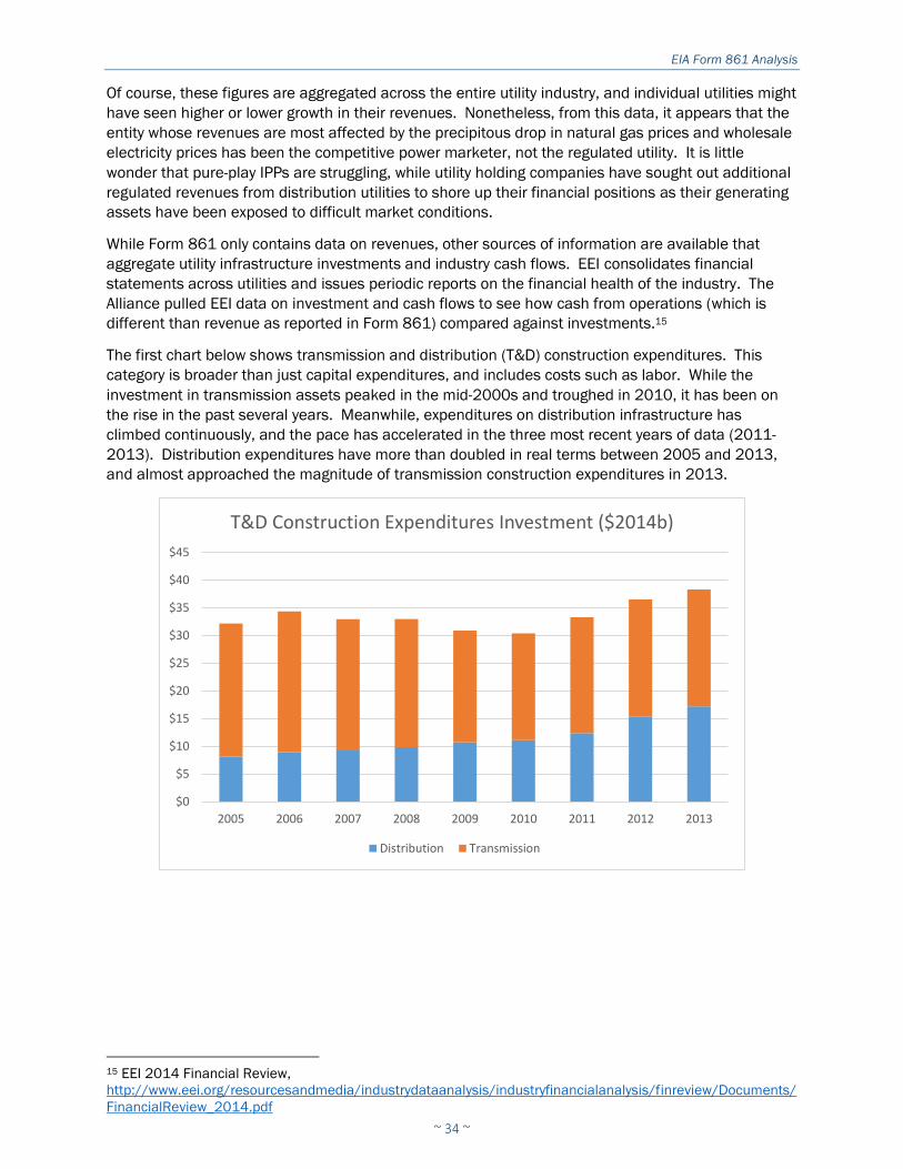
The first chart below shows transmission and distribution (T&D) construction expenditures. This

category is broader than just capital expenditures, and includes costs such as labor. While the

investment in transmission assets peaked in the mid-2000s and troughed in 2010, it has been on

the rise in the past several years. Meanwhile, expenditures on distribution infrastructure has

climbed continuously, and the pace has accelerated in the three most recent years of data (2011-

2013). Distribution expenditures have more than doubled in real terms between 2005 and 2013,

and almost approached the magnitude of transmission construction expenditures in 2013.

15 EEI 2014 Financial Review,

http://www.eei.org/resourcesandmedia/industrydataanalysis/industryfinancialanalysis/finreview/Documents/

FinancialReview_2014.pdf

$0

$5

$10

$15

$20

$25

$30

$35

$40

$45

2005 2006 2007 2008 2009 2010 2011 2012 2013

T&D Construction Expenditures Investment ($2014b)

Distribution Transmission

http://www.eei.org/resourcesandmedia/industrydataanalysis/industryfinancialanalysis/finreview/Documents/FinancialReview_2014.pdf

http://www.eei.org/resourcesandmedia/industrydataanalysis/industryfinancialanalysis/finreview/Documents/FinancialReview_2014.pdf


~ 35 ~

Given rising expenditures and flat revenues, one can anticipate the following chart showing net cash

from operations and free cash flow (FCF).16 While FCF from operations before dividends (the typical

manner in which FCF is reported by companies17) was positive until recently, FCF net of dividends

has been consistently negative over the past decade. This deficit requires that utilities raise

additional money from the debt and equity markets to continue to fund their operations.

Fortunately, the cost of debt has been at historic lows in recent years, and utility credit scores have

remained solid the past several years, enabling access to financial markets at reasonable costs.18

After a steep drop in market capitalization in 2008 (along with much of the rest of the economy), the

EEI Market Capitalization Index has increased from just over $350b to about $630b in 2014.19

Advanced Metering Infrastructure Deployment

One of the major categories of distribution investment in the past several years has been advanced

metering infrastructure (AMI). Form 861 contains information regarding AMI deployment on a utility-

by-utility basis for more than 1,600 utilities. From this information, progress on AMI deployment can

be tracked for a given utility over time, or the current state of AMI deployment can be summarized by

state.

The Alliance took a snapshot of the deployment data, measured as AMI meters as a fraction of total

meters, in 2014. Deployment data was summarized both by the count of utilities in a state, as well

as by the total number of meters in a state. As we can see in the following charts, the apparent

progress of AMI varies considerably depending if one is looking at total utilities or total meters.

When analyzing the data by total utilities, we see that in 30 states, more than half of utilities have

implemented zero AMI meters. In fact, nearly 54% of all utilities who provided data for this section

had installed no AMI meters, while 33% of utilities had installed at least 80% AMI meters. This is a

very different picture when analyzing the data by the counts of meters. In this view, utilities who

installed no AMI only controlled 27% of total meters, while utilities who installed at least 80% AMI

16 Id p 18 17 EEI recognizes this distinction, but reports FCF net of dividends citing the “utility industry’s strong tradition of

dividend payments.” Id p 22. 18 Id p 12 & 71 19 Id p 69

-$100

-$80

-$60

-$40

-$20

$0

$20

$40

$60

$80

$100

2005 2006 2007 2008 2009 2010 2011 2012 2013 2014

Cash Flow Statement Summary ($2014b)

Net Cash from Ops CapEx Dividends FCF FCF net Dividends


~ 36 ~

controlled 38% of all meters. In other words, many small utilities are not installing AMI at all, and

those who are installing AMI tend to serve larger customer populations.

When isolating just IOU utilities, about half report zero AMI metering installations against 22% who

have installed more than 80% AMI meters. Total meter installs are similar to the overall utility

population, with IOUs that installed at least 80% AMI controlling 39% of all meters.

This has an interesting impact on rate design. Since rate design is more a function of a particular

utility, rather than how many customers a utility has, the distribution of utility AMI penetration might

be more relevant than the distribution of utility meter AMI penetration.


~ 37 ~


~ 38 ~


~ 39 ~

Utility Performance by ACEEE Scorecard Quintile Ranking

While operational data was readily comparable back to 2005, collected EE data varied over the

years. In this analysis, the Alliance collated utility EE data back to 2010. While lifecycle savings data

is available in more recent Form 861s, data from 2010-2012 did not include this information. As a

result, the Alliance analyzed annual levels of EE savings and compared them across utilities for the

years 2010-2014. As discussed in the earlier OpenEI narrative, an ACEEE Scorecard rank and

quintile were calculated for each state and applied to this analysis.

The next page shows the absolute and relative levels of EE savings by quintile. Unsurprising, those

utilities in the top quintile states spend more on EE programs than those in the bottom quintiles,

both on an absolute level and a relative level. Notably, the 2nd quintile states have increased their

spending in the past five years, but continued to be dwarfed in spend by the top states. Note that

the right chart normalizes EE spending against total retail sales. This is not the same as the cost of

energy saved, but more closely corresponds to what a customer might be charged per 1,000 kWh

(roughly equal to the average monthly use of a residential customer) for their utility’s EE programs.


~ 40 ~


~ 41 ~

The follow two charts show the incremental savings that are attained, along with an approximation of

the lifecycle cost per kWh saved.20 Again, the trend in total savings is predictable: those states with

higher spending on EE programs save more energy, and in turn tend to get a higher ranking in the

ACEEE Scorecard. However, the magnitude of the difference between the quintiles is striking. The

states in the top quintile saved an average of 5.6x more energy than the states in the bottom

quintile. It is also notable that the 2nd quintile has dramatically increased its savings of late, with

increases in three large states – IL, PA, and MI – driving this quintile’s performance. It is a

testament that when policies align, EE programs – and savings – can be ramped up quickly.

The lifecycle cost data on the right chart is also instructive. While it is true that the cost per lifecycle

kWh saved in the top quintile is higher than the others, it is also true that the states in the top

quintile have been running EE programs for longer and some of the initial inexpensive “low handing

fruit” such as lighting retrofits has already been captured. Further, even in the most expensive

states, the cost per avoided kWh in this data is less than 3 ₵ /kWh. Given that electricity rates are

well in excess of this – even for low-cost states – efficiency clearly costs less than the alternative of

purchasing more supply and building more infrastructure to deliver that supply.

Another observation can be made that shows the impact of policy. The cost per lifecycle kWh saved

in the lowest quintile is roughly the same as that in the 2nd quintile at 1.5 ₵ /kWh, but the 2nd

quintile outperformed the bottom quintile by 320% in 2014 savings. Clearly, the cost of running EE

programs is not a fundamental limiting factor, so something else must be driving the differences.

20 An assumption was made that the average useful life of a utility’s 2013-2014 program’s measures (which

were included in the data from those years) could be applied to its 2010-2012 program measures.


~ 42 ~


~ 43 ~

Policy Impacts on Energy Efficiency Savings

To investigate this observation more deeply, the Alliance considered what policy drivers might be

impacting EE program savings. Three policies were considered: utility regulatory structure (i.e.

vertically integrated or restructured), EERS policies, and revenue decoupling. Each of these policies

was applied at the state level, even if in certain states only some utilities are decoupled or under an

EERS.

The results are intuitive, but the magnitude of the effect is notable. States with EERS and revenue

decoupling have much higher range of average savings than those without these policies. There was

a weak relationship in the data between regulatory structure and EE savings, with competitive supply

states having a slight edge in their savings distribution.

The following table summarizes the results of the policy impacts on EE program savings, and the box-

and-whisker graphs on the following page shows the distribution of savings for each policy.

Policy Has EERS Is Decoupled Is Restructured

Number of States 24 13 17

Average savings with policy 1.22% 1.44% 1.16%

Average savings without policy 0.36% 0.52% 0.55%

Difference 0.86% 0.92% 0.61%

After the impact of each individual policy was determined, we looked to see if there were cumulative

benefits of multiple policies. The relationship is somewhat weak, but generally there appears to be a

benefit of combining policies.

0.00%

0.50%

1.00%

1.50%

2.00%

2.50%

3.00%

3.50%

4.00%

0 1 2 3

EE Savings by Policy Score

None EERS Restructured Decoupled E + R E + D R + D All Weighted Avg


~ 44 ~

Outlier:

RI

3.5%

Outlier:

RI

3.5%

Outlier:

RI

3.5%


~ 45 ~

While the results of the individual policies and even simple combinations of policies are interesting, a

more robust analysis can be performed through a regression analysis. Savings from 2013 and 2014

were regressed on binary variables representing each policy, with the results indicating the strength

and importance of each policy’s contribution to total savings. As foreshadowed from the individual

policy charts, the results show that states with an EERS and decoupling are statistically more likely to

have higher savings than those without, while restructuring was not statistically significant.

Regression

Results

Coefficients Standard Error t Stat P-value

Intercept 0.264% 0.055% 4.757 0.000

EERS 0.627% 0.085% 7.416 0.000

Restructured 0.094% 0.090% 1.045 0.298

Decouple 0.505% 0.097% 5.178 0.000

The regression had an R2 value of 0.59, indicating that roughly 60% of the variation between the

states’ EE savings could be attributed to the variables in the regression. The results show that all

else equal, the presence of an EERS policy will add 0.63% annual savings to a state, while revenue

decoupling will add 0.51% annual savings.

Residential EE Savings Cross-Analysis with OpenEI Database

While the information contained in Form 861 and the OpenEI tariff database are very different, both

databases use the same identifier for a given utility. As mentioned earlier, the tariff database does

not contain participation levels, so it is difficult to draw too many conclusions about the general

existence of tariffs and the savings from those utilities. However, a narrower analysis of residential

fixed charges and residential EE savings was conduction to determine if any relationship existed.

To perform this analysis, the average residential fixed charge for the 409 utilities that reported

residential energy savings was appended to the Form 861 data set, and a scatter plot of 2014

residential EE program savings and average fixed charge was generated. The data show that

occurrences of higher savings are skewed toward utilities with lower fixed charges. Of 205 utilities

with residential EE savings above the median value, 57% had fixed charges below the median value.

And of the 97 utilities with greater than 1% annual residential savings, 65% had fixed charges below

the median value.


~ 46 ~

Concluding Thoughts

The utility industry is moving into unprecedented territory. Sales growth has slowed from historic

norms, and in some states is negative. Infrastructure investments on the distribution side are

increasing. And while revenues from regulated activities have grown, they have grown slowly and

have not kept pace with cash outlays. It is against this backdrop that utilities, customers, and

commissioners must plot a path forward.

EIA Form 861 reveals a number of expected, and perhaps unexpected, results regarding utility EE

programs. Utilities in states with a high ACEEE Scorecard ranking tend to spend more money on EE

programs and realize correspondingly higher savings from those programs. Top tier states save

more than 5 times as much energy as a percentage of sales than bottom tier states, while program

spending remains substantially lower than the alternative cost of supply.

Policies matter in terms of EE performance. Using a regression analysis, the data in Form 861

demonstrates that EERS and rate decoupling policies are statistically significant drivers of energy

savings, and that restructuring, while proving a small benefit for energy savings, it not statistically

significant. Together, these policies contribute about 60% of the expected variation between states.

Rate design is also important, although the direct linkage is harder to analyze with this dataset. To

gain additional insight to a subset of this broader question, the average fixed charge for a residential

customer from the OpenEI database was merged with the Form 861 performance data. There exists

a correlation between lower fixed charges and higher residential energy efficiency performance,

although without detailed participation figures it is difficult to establish a level of causation directly

from this data. That said, there is substantial academic literature that shows that all else equal,

higher fixed charges tend to reduce motivations for consumers to save energy. This leads us into the

third part of our background research.

~ 47 ~

In addition to performing the technical analyses that were described above, the Alliance reviewed

roughly three dozen academic research papers, regulatory orders, and policy whitepapers from a

variety of nationally recognized experts in rate design and energy efficiency policy. We further

reviewed numerous articles from popular industry websites such as E&ENews, Greentech Media,

Utility Dive and regional newspapers following local stories. This section provides a short overview of

several papers that the Alliance found particularly illuminating on the topic at hand. Appendix B

includes a list of sources for all the research papers that were reviewed as part of this effort.

Review of Literature

~ 48 ~

Smart Rate Design for a Smart Future

Lazar, J., and W. Gonzalez. 2015. Regulatory Assistance Project.

Jim Lazar and Wilson Gonzalez wrote Smart Rate Design for a Smart Future to update the basic

principles of rate design that were developed nearly fifty years ago to be more compatible with the

current structure of and challenges facing the modern electricity industry. Lazar and Gonzalez

recognize that rate design is critically important in motivating customer and utility decisions, and that

economically efficient prices underpin good rate design. They note that one estimate ascribes a 15%

difference in energy usage between a progressive and regressive rate design.

Lazar and Gonzalez develop three principles for modern rate design that refresh the classic

Bonbright21 principles in a world with high and increasing DER penetration and customer-sited

backup supply.

Principle 1: A customer should be able to connect to the grid for no more than the cost of

connecting to the grid.

Principle 2: Customers should pay for grid services and power supply in proportion to how

much they use these services and how much power they consume.

Principle 3: Customers who supply power to the grid should be fairly compensated for the full

value of the power they supply.

Applying these principles leads the authors towards time-varying rates and away from high fixed

charge structures. Time differentiated pricing helps more equitably recover costs and send efficient

price signals to consumers to help minimize overall system costs. Further, the authors suggest that

while demand charges based on non-coincident peaks were necessary due to technical limitations

before AMI was deployed, they fail to properly allocate costs based on system use. The general

conclusion of the paper is that time-varying costs are the best way to recover costs and to meet

policy objectives such as energy efficiency.

Lazar and Gonzalez offer a sample rate structure for residential customers that reflect their

principles. Note the small customer charge that only recovers basic customer-related charges and

not any system charges. A small demand charge based on the final line transformer is included, but

the bulk of the revenue is collected through time-varying energy rates along with a critical peak

pricing component.

Rate Element Based On the Cost Of Illustrative Rate

Customer Charge Service Drop, Billing, and Collection Only $4.00/month

Transformer Charge Final Line Transformer $1/kVA/month

Off-Peak Energy Baseload Resources + Transmission and

Distribution $.07/kWh

Mid-Peak Energy Baseload + Intermediate Resources + T&D $.09/kWh

On-Peak Energy Baseload, Intermediate, and Peaking Resources +

T&D $.14/kWh

Critical Peak Energy (or

PTR) Demand Response Resources $.74/kWh

21 Bonbright, J.C. 1961. “Principles of Public Utility Rates.”


~ 49 ~

Designing a New Utility Business Model? Better Understand the Traditional One First

Kihm, S., J. Barrett, and C.J. Bell. 2016. American Council for an Energy-Efficient Economy.

Moving Toward Value in Utility Compensation. Part One – Revenue and Profit.

Kihm, S., R. Lehr, S. Aggarwal, and E. Burgess. 2015. Seventhwave, Western Grid Group, America’s

Power Plan, Utility of the Future Center.

This pair of reports, co-authored by Steve Kihm, discusses the financial drivers that underpin utility

management decisions, and concludes that shareholder value should be the ultimate arbiter of the

financial success of a utility company. The first report (ACEEE) focuses on a commonly

misunderstood motivator of utility investments. The second paper (Seventhwave) asks how

regulators should use this motivating factor to achieve policy goals.

In the ACEEE report, the authors use data from financial markets to corroborate the findings that

when utilities’ returns on equity exceed their cost of equity, they can create shareholder value

through investments. This is not a problem per se, but it does create an incentive for utilities to

invest, as each dollar invested will increase shareholder value. The question for policy makers is

how to best create incentive structures that align the utility’s desire to invest with consumers’ and

society’s desire for positive outcomes.

In the Seventhwave report, Kihm et al. use the basic tenets of corporate finance to demonstrate that

a utility has an incentive to invest when their expected return on equity exceeds their cost of equity.

Using recent rate cases, the authors determine that a typical return on equity is around 10%. Using

book-to-value ratios, they further determine that a typical utility cost of equity is about 7.5%. While

the spread between these two values is currently positive, this was not always the case. During a

period from the mid-1960s through 1980, the return on equity was less than the cost of equity, and

by investing in infrastructure during this time, utility stocks lost billions of dollars’ worth of

shareholder value.

However, in the current regulatory and financing regime, the positive spread between the return on

and cost of equity results in a scenario where utilities create shareholder value every time they

deploy capital. Further, they typically earn the same return regardless of the investment’s value to

customers or to society. Finally, rate cases tend to focus on recovering costs that are historic in

nature, rather than looking at what future value will be delivered through new investments.

Given this, the authors discuss what utility commissioners should do. They do not suggest eroding

the return on equity to the point where utilities have no incentive to invest, but rather to structure

their earning power in a way that aligns with other policy interests that the utility customers may

have. The authors ask two key questions:

What values and services do we want our electric system to provide?

How can we improve the incentives currently provided by regulation to get more of what we

want from electric utilities?

Kihm et al. suggest that regulators have direct control over the return on equity that they allow

utilities to earn (through rate cases), but are only able to influence the cost of that equity (set by the

financial markets). In setting the return on equity, the authors caution commissioners to pay

attention to the magnitude of shareholder value created in dollars, rather than to the return on

equity in percentages.22 They further suggest that performance-based incentives are a good way to

22 This is an important distinction, because the value created from a large return on a small investment (e.g. a

10% return on a $100,000 investment) may be smaller than the value created from a small return on a large

investment (e.g. a 2% return on a $1,000,000).


~ 50 ~

align the incentive for utilities to invest in ways that provide benefits to consumers and society in

additional to bringing value to shareholders.

They also suggest that while commissioners cannot set the cost of equity that the financial market

requires for investment, they can influence the cost by either increasing or decreasing the perceived

riskiness of the utility’s investments. In one example of a utility choosing to invest between a coal

plant, a gas plant, and a wind farm, the authors suggest that a commission could pre-approve

recovery of the costs associated with the wind farm within a certain deviation from the budgeted

costs, while holding the costs associated with the coal plant to a full prudency review. In this

instance, the investment in the wind farm is de-risked relative to the investment in the coal plant.

The concluding thought on this pair of papers is best expressed through one of their quotes:

For investors, it’s all about value, not profit. If utilities can create shareholder value by

investing in certain assets, but can only tread water in a financial sense if they invest in

others, utilities will seek out the value-creating resources. This takes us back to Kahn. It is

not appropriate that all utilities earn returns in excess of the cost of equity on all

investments. Our goal should be to allow such returns only on investments that help to

deliver value to customers and achieve public policy objectives. (Seventhwave, p 17,

emphasis in original)


~ 51 ~

Electric Industry Structure and Regulatory Responses in a High Distributed Energy

Resources Future

Corneli, S., and S. Kihm. 2015. Future Electric Utility Series. Lawrence Berkeley National Laboratory.

Rep. no. 1

The first in the six-part Lawrence Berkeley National Lab “Future Electric Utility Series”, this report

from Steve Corneli and Steve Kihm discusses the pressures of technological innovation and

deployment of distributed energy resources (DER) on the traditional monopoly structure of utility

companies. The authors examine why the traditional model might be breaking down, and whether or

not a regulated monopoly continues to be the socially optimal manner in which to deliver certain

electricity services.

Corneli and Kihm discuss the economic theory behind natural monopoly regulation of utility

companies. In the historic construct, granting utilities service territory monopolies produced a

societally optimal outcome as the economies of scope enabled a single entity to serve the entire

customer base at a lower cost than multiple firms serving the market. But as the cost of DERs has

fallen, it begs a question whether this continues to be the case for all products (e.g. energy, capacity,

integration services) that a distribution utility currently provides its customers. If the answer is yes,

then society is best served by continuing the monopoly supply of these services. However, if the

answer is no, then enabling competition for some of the products may produce better outcomes.

The authors discuss two hypothetical worlds in 2030 in which the challenges of increasing DER

penetration must be addressed by regulators, with each author proposing an alternative solution.

Kihm argues that distribution utilities will continue to play an important role in DER markets,

including the ownership and management of DER assets, but acknowledges that regulators might

have pause about allowing them to compete with third-parties in competitive DER markets. He lays

out a future where DER markets did not “blossom fully of their own accord,” and where some utilities

had an opportunity to pursue cost-effective DERs on their own, while others sought partnerships to

provide integration services to third-party DER providers.

Corneli hypothesizes a future that is defined by competition for DER products and services, primarily

among third-parties, and where the utility role is primarily one of coordination. The primary services

that the distribution utility (as distinct from the bulk power grid) provides in 2030 is “connected

capacity” and “delivered energy.” Connected capacity can be thought as the maximum amount of

power that a user can draw from the distribution grid, while the energy is the volumetric kWh that

can be used by the customer, up to the connected capacity limit. Despite the prevalence and low

cost of DERs, it might still be economical for a customer to maintain some degree of connected

capacity and occasionally purchase energy through the distribution grid. But, in this hypothetical

future, the continue revenue erosion from DERs forced utilities to maintain profitability by focusing

their investments in areas that provided value to customers. Coupled with the development of

simple markets to allow customers to transact for DER services, utilities play a coordinating role in

managing their grid.

Both authors agree that high penetrations of DERs will create changes in today’s utility business

model and will force regulators to define what areas they want to enable utilities to participate. This

debate is currently playing out in the NY REV proceeding, where a focus on competitive markets has

led NYPUC to preclude utilities from owning DERs in most circumstances and to act as the

coordinator.


~ 52 ~

Distribution Systems in a High Distributed Energy Resources Future: Planning, Market

Design, Operation and Oversight

De Martini, P., and L. Kristov. 2015. Future Electric Utility Series. Lawrence Berkeley National Lab.

Rep. no. 2

The second in the six-part Lawrence Berkeley National Lab “Future Electric Utility Series”, this report

from Paul De Martini and Lorenzo Kristov continues the discussion of the impact of DERs on the

traditional monopoly structure of utility companies. Taking a continued deployment of DER as a

given, the authors discuss how utilities and regulators can work to transition from the current

paradigm to a sustainable utility business model in the future.

De Martini and Kristov define the transmission / distribution (T-D) interface as the logical junction to

analyze the operational functions of the power grid of the future. They focus on the distribution grid

operations, and leave aside retail supply functions. In this manner, they define three stages of

distribution system evolution:

1. Grid Modernization – low levels of DER adoption that can be adapted to by existing

system and planning procedures with minimum operational or procedural changes.

2. DER Integration – multi-way power flows begin to require new operational capabilities

and increases the variability of the distribution grid. At the same time, DER penetration

has reached a level where they can begin to provide real-time system benefits.

3. Distributed Markets – the arrival of “peer-to-peer” transactions between DERs and

customers. This stage will require new regulatory frameworks and new market

structures.

The authors detail the potential challenges and benefits that DERs can provide at each stage of the

distribution grid evolution, and continue to discuss how regulators should consider structuring the

utility to manage their integration. They arrive at three potential distribution system operator (DSO)

models, each of which are discussed in turn.

The “Total ISO” model. Here, the transmission-level ISO has full visibility into the distribution

system and manages and optimizes the whole system. The authors find it intellectually

interesting, but impractical to implement.

The “Minimal DSO” model. The transmission-level ISO continues to optimize the whole

system, but only models DERs at the T-D interface level. The DSO plays a significant

coordinating role in managing and dispatching DERs on the distribution system.

The “Market DSO” model. The most active role for the DSO where it either coordinates DER

aggregators or acts as the DER aggregator to present the ISO one virtual DER resource at

each T-D interface. DSOs are responsible for managing load and DER variability within each

local network and coordinate dispatching at the T-D interface

While the second two examples are both seen as potential models for future distribution utilities, the

authors discuss the various tradeoffs between the two models. Physical constraints must always be

followed, and operational reliability may be increased by overbuilding DERs, but at added cost. They

conclude their paper by walking through a process for stakeholders to analyze and define their policy

aims, design the tools needed to account for and monetize DER value, and set up the organizational

structures that are required to attain their policy objectives.


~ 53 ~

Performance-Based Regulation in a High Distributed Energy Resources Future

Lowry, M.N., and T. Woolf. 2016. Future Electric Utility Series. Lawrence Berkeley National Lab. Rep.

no. 3.

Mark Lowry and Tim Woolf penned the third part of the six-part Lawrence Berkeley National Lab

“Future Electric Utility Series.” Building on the previous two reports in the series that laid the

groundwork on the evolving challenges that utilities face in a high DER world, the authors explored

performance-based regulation (PBR) and how it might be suited to meet these challenges.

Lowry and Woolf begin by discussing the incentive problems that exist in traditional cost of service

regulation. These include incentives that vary based on when and how often rate cases are filed,

incentives to increase a utility’s rate base and energy sales, and a disincentive to accommodate

DERs. Additionally, as DER penetrations increase, the risk of revenue erosion can hurt utility

finances at the exact time when a robust grid is needed to integrate additional DERs.

PBR can help solve some of these misaligned incentives. Two common structures are discussed:

multi-year rate plans (MRPs) and performance incentive mechanisms (PIMs). By granting a long-

term rate case (and precluding utilities from coming in for adjustments during the duration of the

MRP) that is tied to specific metrics and often accompanies by an automatic cost inflation

adjustment mechanism, MRPs aim to provide an incentive for a utility to reduce its costs and

increase its efficiency. Common components of MRP include revenue decoupling, shared savings

structures, and cost trackers for capital investments.

PIMs help provide guidance to utilities by setting out specific performance goals and financial

incentives to meet the targeted performance. To implement PIMs, regulators must be clear and

specific in the types and structure of the goals they wish utilities to pursue. These metrics can be

implemented in stages, starting with “scorecard” measurements before graduating to monetized

performance, or beginning with incentives before moving to bi-directional incentives and penalties.

PIMs are often used in conjunction with MRPs to ensure that the utility does not try to cut costs to

the point that degrades service quality.

Britain’s RIIO (Revenues = Incentives + Innovation + Outcomes) is one of the highest profile MRPs

currently in place. In this process, electric and gas utilities operate under an eight-year plan with

revenue decoupling, an inflation-adjustment mechanism, and incentives tied to customer service

and reliability that directly impact utility earnings. RIIO also enables utilities to earn returns on total

expenditures – as opposed to the more traditional return on capital expenditures – to remove

incentives to only invest in projects that increase the rate base.

MRPs and PIMs have advantages and disadvantages from both the customer and utility perspective.

For example, while MRP provide an incentive for utilities to reduce costs and share savings with

customers, they also tend to lead to automatic rate increases. PIMs can help direct investment to

areas where policymakers want focus, but they may entail high administrative costs and be subject

to gaming and manipulation. Regardless of these challenges, PBR in a high DER world can be a

useful tool in the regulator's toolbox.


~ 54 ~

Pathway to a 21st Century Electric Utility

Kind, P.H. 2015. Ceres.

Peter Kind was the author of EEI’s 2013 report Disruptive Challenges that kicked off much of the

current activity around the concept fixed cost recovery. While the intervening years saw considerable

action – both by utilities and by DER advocates – related to increasing fixed charges, Kind released

his late-2015 follow up report against a very different backdrop. Kind acknowledges that the push

towards higher fixed costs over the past several years damaged the relationship between utilities

and their customers, and in this report advocates a return to a more customer-value focus in utility

ratemaking and operations.

Kind sees the distribution utility as the central integrator of resources and stakeholder collaboration

to attain policy goals as expressed by consumers and policy makers. These policy goals include

enhancing reliability and resiliency while maintaining affordability; recognizing the increasing

importance of creating cleaner energy supply; optimizing system energy loads and load factors to

reduce total cost to serve; and focusing on customer value, including the offering of service choice

and easing adoption of DERs.

To attain these goals, Kind lays out four required foundational principles:

The financial viability of utilities must be secured to enable them to fund and support

enhanced capabilities on the grid

Policymakers must define and promote clear policy goals in a comprehensive, integrated

manner

A commitment to engaging and empowering customers is necessary, including access to

third party providers and necessary data

Equitable tariff structures that promote fairness and policy goals must be implemented

Financial viability will be particularly crucial, as estimates suggest that electric utilities will need to

spend between $75 and $100 billion annually to maintain current reliability levels. This is

substantially higher than the $30 billion it generates in operating income, making continued reliance

on market debt a must. Kind also argues that policy makers must clearly define the rules of the

road, so that utilities can react to and plan towards them. These policy objectives should be

constructed in a comprehensive manner and be consistent with jurisdictional divisions that exist.

Customers are increasingly desiring choice in their energy supply, whether from clean generation or

DERs. Kind suggests the current utility investment bias towards capital infrastructure needs to be

shifted to focus on customer value. Finally, he argues that all of this requires that equitable tariff

structures be in place to fairly record costs from those who use the distribution grid.

These principles are satisfied through actions that policy makers implement. Legislation such as

EERS and RPS can send a clear signal as to what is important to states. Regulatory reform, including

multi-year integrated planning at the transmission and distribution level, can anticipate and direct

DERs to their optimal size and location. Tariff structures based on inclining block rates and

bidirectional metering of DER customers help allocate costs, and active DR and TOU rates create

incentives to manage the overall size of the grid.

All of these actions can be managed by developing an accountability and incentive framework that

rewards utilities for creating customer value in addition to shareholder value. Performance-based

ratemaking can include metrics on reliability, customer service, efficiency, and carbon intensity,

while multi-year, forward looking rate cases provide utilities and their investors confidence to deploy

capital.


~ 55 ~

Rate Design for the Distribution Edge: Electricity Pricing for a Distributed Resource Future

Electricity Innovation Lab. 2014. Rocky Mountain Institute

RMI’s report Rate Design for the Distribution Edge focuses on pricing characteristics that will

become increasingly important in a high DER penetration world. While traditional rate structures

that recovered costs through flat variable rates might have worked well in a past with high load

growth and no customer-sited alternatives, they are unlikely to lead to optimal outcomes in a future

where DERs increase in prevalence.

RMI calls for rates to become more sophisticated in response to the current challenges. Specifically,

they suggest three areas in which rates can become more response: attribute unbundling (energy,

capacity, ancillary services), temporal granularity (from flat/block to TOU/dynamic pricing), and

locational granularity (treating all DER the same vs geotargeted pricing).

These three attributes are discussed in both near-term and longer-term scenarios:

Rate Characteristic Near-Term Default or Opt-In Possibilities

Longer-Term, More Sophisticated Possibilities

Attribute Unbundling Demand charges Attribute-based pricing

Temporal Granularity TOU w CPP Pricing Real Time Pricing

Locational Granularity Distribution “Hot Spot” Credits Distribution Locational Marginal Price

Some of the longer-term possibilities require additional metering and systems capability, but as AMI

deployments continue, these rate structures are poised to leverage that investment into delivering

customer value.

RMI caution regulators to closely manage the complexity of the offerings to mass-market (i.e.

residential and small commercial) customers, as rates must offer price signals that are not only

economically efficient, but to which customers are able to understand and reasonably respond.

Regulators must identify the timeline for a transition, and determine how to manage “opt-in” vs. “opt-

out” considerations. They must also work to improve the overall rate design process, increasing

transparency and accessibility to more stakeholders. Importantly, as DER penetration increases,

rate design must anticipate changes to the net load profiles of the system to ensure that peak

periods respond to the shifting loads and generation profiles of customers. Locking in a rate

structure based on today’s peaks may not be useful if the peak shifts after a significant deployment

of DER.


~ 56 ~

Electric Utility Residential Customer Charges and Minimum Bills: Alternative Approaches for

Recovering Basic Distribution Costs

Lazar, J. 2014. The Regulatory Assistance Project.

In this report, Jim Lazar focuses on the distinction between customer-specific charges and system

charges. He suggests that true customer-specific marginal costs, such as billing and collection, are

appropriately recovered through a fixed system charge that is independent of a customer’s usage.

But Lazar notes that utilities have been proposing fixed charges that include other systems

elements, such as poles, transformers, and wires. In his view, collecting these system charges

through a fixed customer charge is not consistent with economic principles, as rates should reflect

the long-run marginal cost of a system, and all distribution plant is marginal in the long run.

A shift to higher fixed charges would have negative effects on low-use customers such as renters,

low income households, and urban residents who rely on gas heating. Lazar also points out that

higher fixed charges will result in lower variable costs, which in turn reduce the incentive for

customers to conserve energy.

One potential alternative to raising fixed charges is to adopt a minimum bill. In this structure, a small

customer charge will still be collected, but the majority of a customer’s costs will remain in an

economically efficient variable rate. For very low-use customers or customers with DG offsetting

most or all of their load, a minimum bill will ensure that they contribute some degree to the recovery

of system costs. Lazar calculates that the difference between a $20 minimum bill and a $20 fixed

charge would result in about 15 times as much additional usage in the fixed charge option.

Lazar also notes that high fixed charges are often discussed in the context of distributed PV

customers. For a customer that offsets most of all of their load through net metering, it is currently

possible that they do not contribute any funds towards the recovery of system costs. A minimum bill

would ensure that they contribute towards these costs, but would not distort rate signals for all

customers in the process as a high fixed charge would.


~ 57 ~

Time-Varying and Dynamic Rate Design

Faruqui, A., R. Hledik, J. Palmer. 2012. Global Power Best Practice Series. Regulatory Assistance

Project and the Brattle Group

Advances in metering technology are opening up new avenues in rate design that did not exist with

legacy meters. Rate designs that vary based on time or system conditions are better as sending

efficient price signals to customers. By altering energy prices based on known or anticipated times

of peak load, customers will have incentives to reduce their own use, thus reducing the total load on

the system, and subsequently reducing the costs of serving all customers. Additionally, with the

increased variability of supply from non-dispatchable resources, dynamic pricing can help load

respond to supply in a more efficient manner.

While TOU rates have been around for decades, their overall participation levels have tended to be

low. Nonetheless, results from pilot programs have demonstrated that these rate structures help

reduce system peaks, in some cases substantially so, as seen in the diagram below. However, there

is not a strong conservation effect from historic TOU rates, as customers tend to simply shift their

energy use rather than reduce it. The authors note that this is an area where additional research will

be useful.

When implementing time-varying rates, the authors recommend a seven-step process:

0. Understand the impacts of current rates. Utilize focus groups and surveys.

1. Develop a consistent and comprehensive set of ratemaking objectives. This should be done

in advance of ratemaking design to ensure outcomes are desired.

2. Identify the menu of possible new rate options. What options are on the table? Is AMI

available?

3. Perform preliminary assessment of potential impacts. Develop rate designs from real data.

4. Conduct preliminary market research. Investigate customer response to initial designs.

5. Conduct time-varying rate pilots. Include shadow bills and monitor impact on low income

customers.

6. Full-scale deployment of innovative rates. Identify rates that best align with policy objectives

and more to roll out more broadly

~ 58 ~

ACEEE Scorecard Ranking

State 2011 2012 2013 2014 2015 Average Rank ACEEE Quintile

Massachusetts 1 1 1 1 1 1 1 1st

California 2 2 2 2 2 2 2 1st

Oregon 4 4 4 3 4 3.8 3 1st

Vermont 5 5 7 3 3 4.6 4 1st

Rhode Island 5 7 6 3 4 5 5 1st

New York 3 3 3 7 9 5 6 1st

Connecticut 8 6 5 6 6 6.2 7 1st

Washington 5 8 8 8 8 7.4 8 1st

Maryland 10 9 9 9 7 8.8 9 1st

Minnesota 8 9 11 10 10 9.6 10 1st

Iowa 11 11 12 14 12 12 11 2nd

Illinois 17 14 10 11 10 12.4 12 2nd

Colorado 12 14 16 13 12 13.4 13 2nd

Michigan 17 12 12 12 14 13.4 14 2nd

Arizona 17 12 12 15 17 14.6 15 2nd

Maine 12 25 16 16 14 16.6 16 2nd

New Jersey 15 16 12 19 21 16.6 17 2nd

Hawaii 12 18 20 17 19 17.2 18 2nd

Wisconsin 16 17 23 17 22 19 19 2nd

Pennsylvania 25 20 19 20 17 20.2 20 2nd

New Hampshire 21 18 21 22 20 20.4 21 3rd

Utah 17 21 24 23 23 21.6 22 3rd

District of Columbia 22 29 30 21 14 23.2 23 3rd

Ohio 24 22 18 25 27 23.2 24 3rd

North Carolina 27 22 24 24 24 24.2 25 3rd

Delaware 31 27 22 25 24 25.8 26 3rd

New Mexico 27 27 24 25 31 26.8 27 3rd

Florida 27 29 27 28 27 27.6 28 3rd

Idaho 26 22 31 30 29 27.6 29 3rd

Nevada 22 31 33 29 31 29.2 30 3rd

Montana 35 25 29 31 31 30.2 31 4th

Texas 33 33 33 34 26 31.8 32 4th

Tennessee 30 32 31 38 31 32.4 33 4th

Indiana 32 33 27 40 38 34 34 4th

Virginia 34 37 36 35 31 34.6 35 4th

Kentucky 37 36 39 33 29 34.8 36 4th

Arkansas 38 37 37 31 31 34.8 37 4th

Georgia 36 33 33 35 37 34.8 38 4th

Oklahoma 47 39 37 35 38 39.2 39 4th

Alabama 43 40 39 39 41 40.4 40 4th

South Carolina 46 40 39 42 40 41.4 41 5th

Nebraska 40 42 44 42 42 42 42 5th

Kansas 48 45 39 40 45 43.4 43 5th

Missouri 44 43 43 44 44 43.6 44 5th

Louisiana 40 43 44 44 48 43.8 45 5th

Alaska 38 46 47 47 42 44 46 5th

West Virginia 44 49 46 46 45 46 47 5th

South Dakota 42 46 47 49 48 46.4 48 5th

Mississippi 49 51 47 47 47 48.2 49 5th

Wyoming 50 48 50 50 50 49.6 50 5th

North Dakota 51 50 51 51 51 50.8 51 5th

Appendix B

~ 59 ~

Benjamin, R., M. Kito, R. Mutialu, G. Petlin, P. Phillips, and J. Rahman. 2014. “Energy Division Staff

Proposal on Residential Rate Reform,” Staff Proposal for Residential Rate Reform in Compliance

with R.12-06-013 and Assembly Bill 327. California Public Utilities Commission.

http://www.cpuc.ca.gov/uploadedFiles/CPUC_Website/Content/Utilities_and_Industries/Energy

/Reports_and_White_Papers/FINAL_ED_Staff_Proposal_RateReformforWeb5_9_2014.pdf

Bird, L., C. Davidson, J. McLaren, and J. Miller. 2015. “Impact of Rate Design Alternatives on

Residential Solar Customer Bills: Increased Fixed Charges, Minimum Bills and Demand-Based

Rates.” National Renewable Energy Laboratory. Rep. no. NREL/TP-6A20-64850.

http://www.nrel.gov/docs/fy15osti/64850.pdf

Bonbright, J.C. 1961. “Principles of Public Utility Rates.” Powell Goldstein LLP.

http://media.terry.uga.edu/documents/exec_ed/bonbright/principles_of_public_utility_rates.pdf

Borenstein, S. 2012. Effective and Equitable Adoption of Opt-In Residential Dynamic Electricity

Pricing. Energy Institute at Haas. https://ei.haas.berkeley.edu/research/papers/WP229.pdf

Cappers, P., J. MacDonald, J. Page, J. Potter, E. Stewart. 2016. “Future Opportunities and Challenges

with Using Demand Response as a Resource in Distribution System Operation and Planning

Activities.” Lawrence Berkeley National Laboratory. Rep. no. LBNL-1003951.

https://emp.lbl.gov/publications/future-opportunities-and-challenges

Corneli, S., and S. Kihm. 2015. “Electric Industry Structure and Regulatory Responses in a High

Distributed Energy Resources Future.” Future Electric Utility Series. Lawrence Berkeley National

Laboratory. Rep. no. 1. https://emp.lbl.gov/future-electric-utility-regulation-series

Corneli, S. and S. Kihm. N.d. “Distributed Energy Resources: Industry Structure, Institutions, and

Regulatory Responses.” Future Electric Utility Series. Lawrence Berkeley National Laboratory.

PowerPoint. https://emp.lbl.gov/future-electric-utility-regulation-series

De Martini, P., and L. Kristov. 2015. “Distribution Systems in a High Distributed Energy Resources

Future: Planning, Market Design, Operation and Oversight.” Future Electric Utility Series.

Lawrence Berkeley National Lab. Rep. no. 2. https://emp.lbl.gov/future-electric-utility-regulation-

series

De Martini, P., and L. Kristov. 2015. “Distribution Systems in a High Distributed Energy Resources

Future: Planning, Market Design, Operation and Oversight.” Future Electric Utility Series.

Lawrence Berkeley National Lab. Webinar presentation, 13 November 2015.

https://emp.lbl.gov/future-electric-utility-regulation-series

Electricity Innovation Lab. 2013. “New Business Models for the Distribution Edge: The Transition

from Value Chain to Value Constellation.” Rocky Mountain Institute.

http://www.rmi.org/New_Business_Models

Electricity Innovation Lab. 2014. “Rate Design for the Distribution Edge: Electricity Pricing for a

Distributed Resource Future.” Rocky Mountain Institute. http://www.rmi.org/elab_rate_design

Faruqui, A., R. Hledik, J. Palmer. 2012. “Time-Varying and Dynamic Rate Design.” Global Power Best

Practice Series. Regulatory Assistance Project and the Brattle Group.

www.raponline.org/document/download/id/5131

http://www.cpuc.ca.gov/uploadedFiles/CPUC_Website/Content/Utilities_and_Industries/Energy/Reports_and_White_Papers/FINAL_ED_Staff_Proposal_RateReformforWeb5_9_2014.pdf

http://www.cpuc.ca.gov/uploadedFiles/CPUC_Website/Content/Utilities_and_Industries/Energy/Reports_and_White_Papers/FINAL_ED_Staff_Proposal_RateReformforWeb5_9_2014.pdf

http://www.nrel.gov/docs/fy15osti/64850.pdf

http://media.terry.uga.edu/documents/exec_ed/bonbright/principles_of_public_utility_rates.pdf

https://ei.haas.berkeley.edu/research/papers/WP229.pdf

https://emp.lbl.gov/publications/future-opportunities-and-challenges






http://www.rmi.org/New_Business_Models

http://www.rmi.org/elab_rate_design

http://www.raponline.org/document/download/id/5131

Appendix B

~ 60 ~

Florio, M.P. 2016. Assigned Commissioner’s Ruling Introducing a Draft Regulatory Incentives

Proposal for Discussion and Comment. Public Utilities Commission of the State of California.

http://www.cpuc.ca.gov/WorkArea/DownloadAsset.aspx?id=7799

Hledik, R. 2015. “Rolling Out Residential Demand Charges.” The Brattle Group. EUCI Residential

Demand Charges Summit.

http://www.brattle.com/system/publications/pdfs/000/005/170/original/Rolling_Out_Residen

tial_Demand_Charges_Hledik_EUCI.pdf?1431628444

Institute for Electric Innovation. 2014. State Electric Efficiency Regulatory Frameworks. IEI Report.

The Edison Foundation.

http://www.edisonfoundation.net/iei/Documents/IEI_stateEEpolicyupdate_1214.pdf

Ito, K. 2014. “Do Consumers Respond to Marginal or Average Price? Evidence from Nonlinear

Electricity Pricing.” The American Economic Review. Vol. 104, No. 2. Pp. 537-63.

http://home.uchicago.edu/ito/Ito_Marginal_Average_AER.pdf

Hledik, R. “Rediscovering Residential Demand Charges.” The Electricity Journal. Aug./Sept. 27.7,

2014.

Kihm, S., J. Barrett, and C.J. Bell. 2016. “Designing a New Utility Business Model? Better Understand

the Traditional One First.” American Council for an Energy-Efficient Economy. Washington, D.C.

https://www.seventhwave.org/sites/default/files/2014-aceee-ss-kihm.pdf

Kihm, S., R. Lehr, S. Aggarwal, and E. Burgess. 2015. Moving Toward Value in Utility Compensation.

Part One – Revenue and Profit. Seventhwave, Western Grid Group, America’s Power Plan, Utility

of the Future Center. https://www.seventhwave.org/sites/default/files/you-get-what-you-pay-for-

part-one-2015.pdf

Kind, P.H. 2015. “Pathway to a 21st Century Electric Utility.” Ceres.

http://www.ceres.org/resources/reports/pathway-to-a-21st-century-electric-utility

Kind, P. 2013. Disruptive Challenges: Financial Implications and Strategic Responses to a Changing

Retail Electric Business. Edison Electric Institute. Washington, D.C.

http://www.eei.org/ourissues/finance/documents/disruptivechallenges.pdf

Lazar, J. 2013. “Rate Design Where Advanced Metering Infrastructure Has Not Been Fully Deployed.”

Global Power Best Practice Series. Regulatory Assistance Project.

www.raponline.org/document/download/id/6516

Lazar, J. 2014. “Electric Utility Residential Customer Charges and Minimum Bills: Alternative

Approaches for Recovering Basic Distribution Costs.” The Regulatory Assistance Project.

Available at: https://www.raponline.org/document/download/id/7361

Lazar, J., and W. Gonzalez. 2015. “Smart Rate Design for a Smart Future.” Regulatory Assistance

Project. Available at: http://www.raponline.org/document/download/id/7680

Lowry, M.N., and T. Woolf. 2016. “Performance-Based Regulation in a High Distributed Energy

Resources Future.” Future Electric Utility Series. Lawrence Berkeley National Lab. Rep. no. 3.

https://emp.lbl.gov/publications/performance-based-regulation-in-a-hig

Lowry, M.N., and T. Woolf. 2016. “Performance-Based Regulation in a High Distributed Energy

Resources Future.” Future Electric Utility Series. Lawrence Berkeley National Lab. Webinar

presentation, 27 January 2016. https://emp.lbl.gov/publications/performance-based-regulation-

in-a-hig

http://www.cpuc.ca.gov/WorkArea/DownloadAsset.aspx?id=7799

http://www.brattle.com/system/publications/pdfs/000/005/170/original/Rolling_Out_Residential_Demand_Charges_Hledik_EUCI.pdf?1431628444

http://www.brattle.com/system/publications/pdfs/000/005/170/original/Rolling_Out_Residential_Demand_Charges_Hledik_EUCI.pdf?1431628444

http://www.edisonfoundation.net/iei/Documents/IEI_stateEEpolicyupdate_1214.pdf

http://home.uchicago.edu/ito/Ito_Marginal_Average_AER.pdf

https://www.seventhwave.org/sites/default/files/2014-aceee-ss-kihm.pdf

https://www.seventhwave.org/sites/default/files/you-get-what-you-pay-for-part-one-2015.pdf

https://www.seventhwave.org/sites/default/files/you-get-what-you-pay-for-part-one-2015.pdf

http://www.ceres.org/resources/reports/pathway-to-a-21st-century-electric-utility

http://www.eei.org/ourissues/finance/documents/disruptivechallenges.pdf


https://www.raponline.org/document/download/id/7361





Appendix B

~ 61 ~

National Action Plan for Energy Efficiency. 2007. Aligning Utility Incentives with Investment in Energy

Efficiency. Prepared by Val R. Jensen, ICF International. www.epa.gov/eeactionplan

Neme, C., and J. Grevatt. 2016. “The Next Quantum Leap in Efficiency: 30 Percent Electric Savings in

Ten Years.” The Regulatory Assistance Project. Available at:

http://www.raponline.org/document/download/id/7944.

Nowak, S., B. Baatz, A. Gillro, M. Kushler, M. Molina, and D. York. 2015. “Beyond Carrots for Utilities:

A National Review of Performance Incentives for Energy Efficiency.” American Council for an

Energy-Efficient Economy. Washington, D.C. Rep. no. U1504. http://aceee.org/beyond-carrots-

utilities-national-review

Russell, C., B. Baatz, R. Cluett, and J. Amann. 2015. “Recognizing the Value of Energy Efficiency’s

Multiple Benefits.” American Council for Energy Efficiency. Washington, D.C. Rep. no. IE1502.

http://aceee.org/research-report/ie1502

Stanton, T. 2015. “Distributed Energy Resources: Status Report on Evaluating Proposals and

Practices for Electric Utility Rate Design.” National Regulatory Research Institute. Rep. no. 15-08.

http://nrri.org/download/nrri-15-08-rate-design-for-der/

Tierney, S.F. 2016. “The Value of “DER” to “D”: The Role of Distributed Energy Resources in

Supporting Local Electric Distribution System Reliability.” Analysis Group, Inc. Available at:

http://www.cpuc.ca.gov/uploadedFiles/CPUC_Public_Website/Content/About_Us/Organization/

Divisions/Policy_and_Planning/Thought_Leaders_Events/Tierney%20White%20Paper%20-

%20Value%20of%20DER%20to%20D%20-%203-30-2016%20FINAL.pdf

Whited, M., T. Wolf, and A. Napoleon. 2015. “Utility Performance Incentive Mechanisms: A Handbook

for Regulators.” Synapse Energy Economics, Inc. http://www.synapse-

energy.com/sites/default/files/Utility%20Performance%20Incentive%20Mechanisms%2014-

098_0.pdf

http://www.epa.gov/eeactionplan


http://aceee.org/beyond-carrots-utilities-national-review

http://aceee.org/beyond-carrots-utilities-national-review

http://aceee.org/research-report/ie1502

http://nrri.org/download/nrri-15-08-rate-design-for-der/

http://www.cpuc.ca.gov/uploadedFiles/CPUC_Public_Website/Content/About_Us/Organization/Divisions/Policy_and_Planning/Thought_Leaders_Events/Tierney%20White%20Paper%20-%20Value%20of%20DER%20to%20D%20-%203-30-2016%20FINAL.pdf



http://www.synapse-energy.com/sites/default/files/Utility%20Performance%20Incentive%20Mechanisms%2014-098_0.pdf



Date post:	03-Jan-2022
Category:	Documents
Upload:	others
View:	1 times
Download:	0 times