31
AS.110.109: Calculus II (Eng) Review session Midterm 1 Yi Wang, Johns Hopkins University Fall 2017

AS.110.109: Calculus II (Eng)
Review session Midterm 1
Yi Wang, Johns Hopkins University
Fall 2017
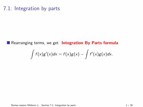
7.1: Integration by parts
� Rearranging terms, we get Integration By Parts formula∫f (x)g ′(x)dx = f (x)g(x)−
∫f ′(x)g(x)dx .
Review session Midterm 1, Section 7.1: Integration by parts 1 / 30
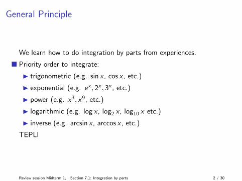
General Principle
We learn how to do integration by parts from experiences.
� Priority order to integrate:
I trigonometric (e.g. sin x , cos x , etc.)
I exponential (e.g. ex , 2x , 3x , etc.)
I power (e.g. x3, x9, etc.)
I logarithmic (e.g. log x , log2 x , log10 x etc.)
I inverse (e.g. arcsin x , arccos x , etc.)
TEPLI
Review session Midterm 1, Section 7.1: Integration by parts 2 / 30
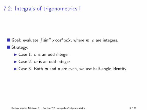
7.2: Integrals of trigonometrics I
� Goal: evaluate∫
sinm x cosn xdx , where m, n are integers.
� Strategy:
I Case 1. n is an odd integer
I Case 2. m is an odd integer
I Case 3. Both m and n are even, we use half-angle identity.
Review session Midterm 1, Section 7.2: Integrals of trigonometrics I 3 / 30
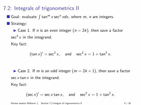
7.2: Integrals of trigonometrics II
� Goal: evaluate∫
tanm x secn xdx , where m, n are integers.
� Strategy:
I Case 1. If n is an even integer (n = 2k), then save a factor
sec2 x in the integrand.
Key fact:
(tan x)′ = sec2 x , and sec2 x = 1 + tan2 x .
I Case 2. If m is an odd integer (m = 2k + 1), then save a factor
sec x tan x in the integrand.
Key fact:
(sec x)′ = sec x tan x , and sec2 x = 1 + tan2 x .
Review session Midterm 1, Section 7.2 Integral of trigonometrics II 4 / 30

7.3: Trigonometric substitution
3 different substitutions we usually use:
I√a2 − x2 = a sin t by substituting x = a cos t
and using identity 1− cos2 t = sin2 t.
I√a2 + x2 = a sec t by substituting x = a tan t
and using identity 1 + tan2 t = sec2 t.
I√x2 − a2 = a tan t by substituting x = a sec t
and using identity sec2 t − 1 = tan2 t.
Review session Midterm 1, Section 7.2 Integral of trigonometrics II 5 / 30

7.4: Integration of rational functions
A rational function is a function of the form:
f (x) =P(x)
Q(x),
where P(x) and Q(x) are polynomials in x .
P(x) = anxn + an−1x
n−1 + · · ·+ a0.
Q(x) = bmxm + bm−1x
m−1 + · · ·+ b0.
How to express a rational function as a linear combination of
partial fractions?
Review session Midterm 1, Section 7.2 Integral of trigonometrics II 6 / 30

7.4: Integration of rational functions
Definition
f (x) = P(x)Q(x) is called proper if deg(P(x)) < deg(Q(x)).
Otherwise, it is called improper.
A rational function can always be written as:
f (x) = a polynomial function + a proper rational function.
Review session Midterm 1, Section 7.2 Integral of trigonometrics II 7 / 30

7.4: Integration of rational functions
Why?
If f (x) is improper, then we use Q(x) to divide P(x) getting
P(x) = S(x)Q(x) + R(x)
where S(x) and R(x) are polynomials, such that
deg(R(x)) < deg(Q(x)). Then
f (x) =P(x)
Q(x)= S(x) +
R(x)
Q(x).
with R(x)Q(x) being proper.
It is similar to the division of integers!!
Review session Midterm 1, Section 7.2 Integral of trigonometrics II 8 / 30
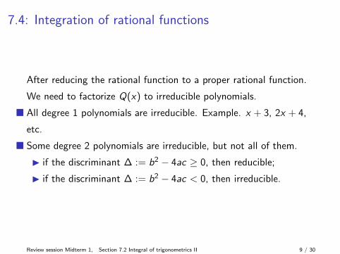
7.4: Integration of rational functions
After reducing the rational function to a proper rational function.
We need to factorize Q(x) to irreducible polynomials.
� All degree 1 polynomials are irreducible. Example. x + 3, 2x + 4,
etc.
� Some degree 2 polynomials are irreducible, but not all of them.
I if the discriminant ∆ := b2 − 4ac ≥ 0, then reducible;
I if the discriminant ∆ := b2 − 4ac < 0, then irreducible.
Review session Midterm 1, Section 7.2 Integral of trigonometrics II 9 / 30

7.4: Integration of rational functions
If P(x) has degree≥ 3, it can always be factored into a product:
P(x) = P1(x) · · ·Pk(x),
where each Pi (x) is a irreducible polynomial with degree ≤ 2.
Pi is either of degree 1, or of degree 2 and ∆ < 0.
Review session Midterm 1, Section 7.2 Integral of trigonometrics II 10 / 30

7.4: Integration of rational functions
To integrate a rational function, we factorize the denominator
Q(x):
Q(x) = Q1(x) · · ·Qk(x).
Case 1. Q(x) is a product of distinct linear factors.R(x)Q(x) takes the form
A1
a1x + b1+ · · ·+ Ak
akx + bk
.
� Example 7.∫
x(x+1)(x+2)dx
x
(x + 1)(x + 2)=
A1
x + 1+
A2
x + 2.
Review session Midterm 1, Section 7.2 Integral of trigonometrics II 11 / 30

7.4: Integration of rational functions
Case 2. Q(x) is a product of linear factors, some of which are
repeated.
Suppose Q(x) contains a term (a1x + b1)r1 . Instead of A1a1x+b1
, we
would haveA1
a1x + b1+ · · ·+ Ar1
(a1x + b1)r1.
For another repeated factor, say (a2x + b2)r2 , we have
B1
a2x + b2+ · · ·+ Br2
(a2x + b2)r2.
Review session Midterm 1, Section 7.2 Integral of trigonometrics II 12 / 30
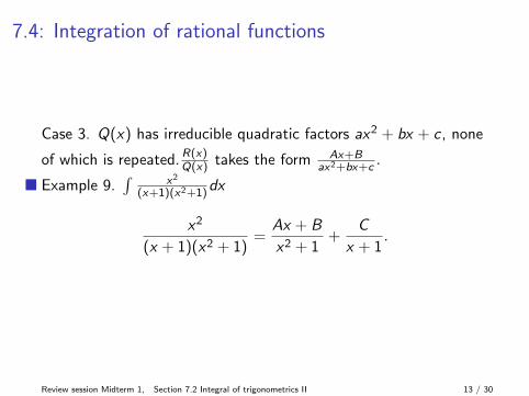
7.4: Integration of rational functions
Case 3. Q(x) has irreducible quadratic factors ax2 + bx + c , none
of which is repeated.R(x)Q(x) takes the form Ax+B
ax2+bx+c.
� Example 9.∫
x2
(x+1)(x2+1)dx
x2
(x + 1)(x2 + 1)=
Ax + B
x2 + 1+
C
x + 1.
Review session Midterm 1, Section 7.2 Integral of trigonometrics II 13 / 30

7.4: Integration of rational functions
Case 4. Q(x) has irreducible quadratic factors ax2 + bx + c , some
of which is repeated. For example. if there is a factor∫
1(x2+a2)r
dx
in Q(x). Then in the decomposition, there are following terms inR(x)Q(x) : (of course, there are other terms corresponding to other
factors of Q.)∫A1x + B1
(x2 + a2)1dx + · · ·+ Arx + Br
(x2 + a2)rdx . (1)
Integration of∫
Ar(x2+a2)r
dx is easy, but that of∫
Br(x2+a2)r
dx might
be complicated.
Review session Midterm 1, Section 7.2 Integral of trigonometrics II 14 / 30
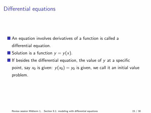
Differential equations
� An equation involves derivatives of a function is called a
differential equation.
� Solution is a function y = y(x).
� If besides the differential equation, the value of y at a specific
point, say x0 is given: y(x0) = y0 is given, we call it an initial value
problem.
Review session Midterm 1, Section 9.1: modeling with differential equations 15 / 30

Geometric meaning of general solution
Each solution is a curve on the xy -plane.
The set of general solution is a family of (infinitely many) curves
on the xy -plane.
Geometrically, the initial condition has the effect of isolating the
integral curve that passes through the point (x0, y0).
Review session Midterm 1, Section 9.1: modeling with differential equations 16 / 30

Population of an animal
Assumption: The population grows at a rate proportional to the
size of the population.
The population model is given by
dP
dt= kP.
Review session Midterm 1, Section 9.1: modeling with differential equations 17 / 30

Population of an animal
In nature, making assumptions that are the most suitable for the
reality is the key to understand the problem.
If P is small, dPdt = kP.
If P > M, dPdt < 0.
A simple modification would be
dP
dt= kP(t)(1− P(t)
M).
Review session Midterm 1, Section 9.1: modeling with differential equations 18 / 30
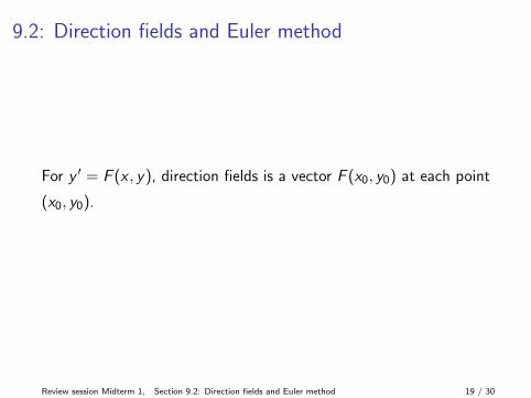
9.2: Direction fields and Euler method
For y ′ = F (x , y), direction fields is a vector F (x0, y0) at each point
(x0, y0).
Review session Midterm 1, Section 9.2: Direction fields and Euler method 19 / 30
9.3: Separable Equations
An equation is separable if one can use algebra to separate the two
variables, so that each side of the equation only contains 1 variable.
Review session Midterm 1, Section 9.3: Separable Equations 20 / 30

Example
Example. Find all the solutions to
y ′ = 2x(1− y)2.
Solution: First note that there is a constant solution y ≡ 1.
Next we use separation method as above
⇒ dy
(1− y)2= 2xdx .
Then integrate both sides,
⇒ 1
1− y= x2 + C .
⇒ y = 1− 1
x2 + C.
This together with y ≡ 1 are the general solutions.Review session Midterm 1, Section 9.3: Separable Equations 21 / 30

Example 6 Orthogonal trajectories.
Take a family of curves x = ky2, where k is any constant. Find
another family of curves such that any member of this family
intersects any given one at a right angle.
x = ky2
⇒ dy
dx=
1
2ky=
y
2x.
The orthogonal trajectories satisfy the differential equation:
dy
dx= −2x
y.
⇒∫
ydy = −∫
2xdx .
⇒ x2 +y2
2= C , C > 0.
Review session Midterm 1, Section 9.3: Separable Equations 22 / 30

Linear equations
A first order linear differential equation is
dy
dx+ P(x)y = Q(x).
Review session Midterm 1, Section 9.5: Linear equations 23 / 30
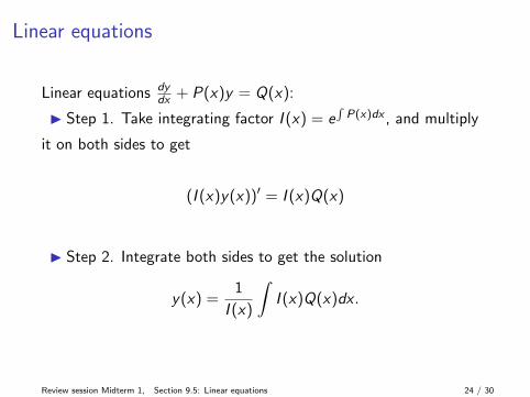
Linear equations
Linear equations dydx + P(x)y = Q(x):
I Step 1. Take integrating factor I (x) = e∫P(x)dx , and multiply
it on both sides to get
(I (x)y(x))′ = I (x)Q(x)
I Step 2. Integrate both sides to get the solution
y(x) =1
I (x)
∫I (x)Q(x)dx .
Review session Midterm 1, Section 9.5: Linear equations 24 / 30
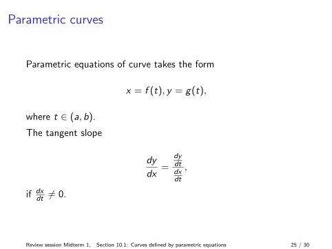
Parametric curves
Parametric equations of curve takes the form
x = f (t), y = g(t),
where t ∈ (a, b).
The tangent slope
dy
dx=
dydtdxdt
,
if dxdt 6= 0.
Review session Midterm 1, Section 10.1: Curves defined by parametric equations 25 / 30

Calculus with parametric curves
Tangent line equation at t = t0 is given by
y(x) = slope · (x − x(t0)) + y(t0).
I At points where dydx = 0, the tangent line is horizontal.
I At points where dydx = ±∞, the tangent line is vertical.
Review session Midterm 1, Section 10.2: Calculus with parametric curves 26 / 30

Calculus with parametric curves
� Second order derivative is
d2y
dx2=
d
dx(dy
dx) =
ddt (dydx )
dxdt
.
Review session Midterm 1, Section 10.2: Calculus with parametric curves 27 / 30
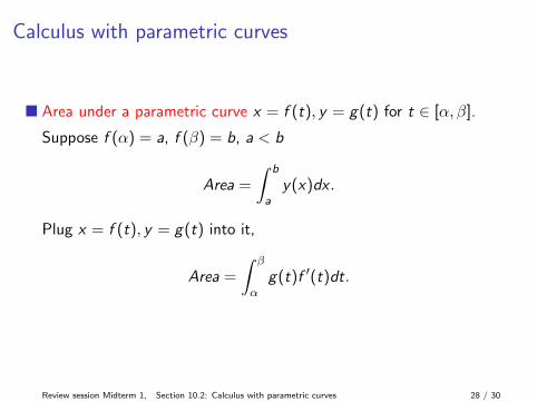
Calculus with parametric curves
� Area under a parametric curve x = f (t), y = g(t) for t ∈ [α, β].
Suppose f (α) = a, f (β) = b, a < b
Area =
∫ b
ay(x)dx .
Plug x = f (t), y = g(t) into it,
Area =
∫ β
αg(t)f ′(t)dt.
Review session Midterm 1, Section 10.2: Calculus with parametric curves 28 / 30

Calculus with parametric curves
� Arc length
Using x = f (t), y = g(t) for t ∈ [α, β],
L =
∫ β
α
√(f ′(t))2 + (g ′(t))2dt. (2)
Review session Midterm 1, Section 10.2: Calculus with parametric curves 29 / 30
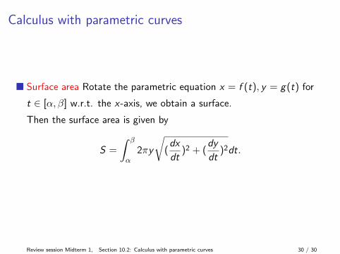
Calculus with parametric curves
� Surface area Rotate the parametric equation x = f (t), y = g(t) for
t ∈ [α, β] w.r.t. the x-axis, we obtain a surface.
Then the surface area is given by
S =
∫ β
α2πy
√(dx
dt)2 + (
dy
dt)2dt.
Review session Midterm 1, Section 10.2: Calculus with parametric curves 30 / 30


