Asian Development Bank Institute · adbi working paper series . urbanization, energy consumption,...

ADBI Working Paper Series

URBANIZATION, ENERGY CONSUMPTION, AND POLLUTANT EMISSION IN ASIAN DEVELOPING ECONOMIES: AN EMPIRICAL ANALYSIS

Ruhul Salim, Shuddhasattwa Rafiq, and Sahar Shafiei

No. 718 April 2017

Asian Development Bank Institute

The Working Paper series is a continuation of the formerly named Discussion Paper series; the numbering of the papers continued without interruption or change. ADBI’s working papers reflect initial ideas on a topic and are posted online for discussion. ADBI encourages readers to post their comments on the main page for each working paper (given in the citation below). Some working papers may develop into other forms of publication.

Unless otherwise stated, boxes, figures and tables without explicit sources were prepared by the authors.

Suggested citation:

Salim, R., S. Rafiq, and S. Shafiei. 2017. Urbanization, Energy Consumption, and Pollutant Emission in Asian Developing Economies: An Empirical Analysis. ADBI Working Paper 718. Tokyo: Asian Development Bank Institute. Available: https://www.adb.org/publications/urbanization-energy-consumption-pollutant-asian-developing-economies Please contact the authors for information about this paper.

Email: [email protected]

Ruhul Salim is associate professor of economics, Curtin Business School, Curtin University. Shuddhasattwa Rafiq is lecturer, School of Accounting, Finance, and Economics, Deakin University. Sahar Shafiei is research assistant, School of Economics & Finance, Curtin University. The views expressed in this paper are the views of the author and do not necessarily reflect the views or policies of ADBI, ADB, its Board of Directors, or the governments they represent. ADBI does not guarantee the accuracy of the data included in this paper and accepts no responsibility for any consequences of their use. Terminology used may not necessarily be consistent with ADB official terms. Working papers are subject to formal revision and correction before they are finalized and considered published.

Asian Development Bank Institute Kasumigaseki Building, 8th Floor 3-2-5 Kasumigaseki, Chiyoda-ku Tokyo 100-6008, Japan Tel: +81-3-3593-5500 Fax: +81-3-3593-5571 URL: www.adbi.org E-mail: [email protected] © 2017 Asian Development Bank Institute

ADBI Working Paper 718 Salim, Rafiq, and Shafiei

Abstract This paper aims to investigate the effects of urbanization, renewable and non-renewable energy consumption, trade liberalization, and economic growth on pollutant emissions and energy intensity in selected Asian developing countries from 1980 to 2010. We use both linear and nonlinear panel data econometric techniques and employ the recently introduced mean group estimation methods, allowing for heterogeneity and cross-sectional dependence. However, to check robustness of our panel results, we also apply the autoregressive distributed lag bound testing approach to country-level data. In addition, the relationship between affluence and CO2 emissions is examined in the context of the Environmental Kuznets Curve (EKC) hypothesis. The estimation results identify population, affluence, and non-renewable energy consumption as the main factors in pollutant emissions in Asian countries. However, the results of the EKC hypothesis show that when countries achieve a certain level of economic growth, their emissions tend to decline. Whereas nonlinear results show that renewable energy, urbanization, and trade liberalization reduce emissions, linear estimations do not confirm such outcomes. Thus, substitution of non-renewable for renewable energy consumption, as well as cautious and planned urbanization programs, and more liberal trading regimes may be viable options for the sustainable growth of these emerging Asian economies. Keywords: renewable energy consumption, urbanization, pollutant emissions, openness, EKC hypothesis, panel data JEL Classification: Q2, E4, C33


Contents 1. INTRODUCTION ....................................................................................................... 1

2. URBANIZATION, EMISSION AND ENERGY INTENSITY: A CRITICAL REVIEW OF THE LITERATURE ........................................................... 2

3. ANALYTICAL FRAMEWORK .................................................................................... 4

4. DATA SOURCES AND DIAGNOSTIC TESTS ........................................................... 5

5. ANALYSIS OF EMPIRICAL RESULTS ...................................................................... 9

5.1 Analysis of the Impact on Pollutant Emissions ............................................... 9 5.2 Analysis of Impact on Energy Intensity ......................................................... 12 5.3 Analysis of Cross-regime Estimations .......................................................... 15 5.4 A Further Investigation ................................................................................. 16

6. CONCLUSION AND POLICY IMPLICATIONS ........................................................ 20

REFERENCES ................................................................................................................... 21


1. INTRODUCTION Urbanization is taking place in an unprecedented speed and scale in developing countries. It took approximately 150 years for Europe’s urbanization rate to increase from 10% to 50%; in most Asian developing countries, that same shift is currently occurring in a time span that is one-third as long. A United Nations report reveals that approximately 54% of the world’s population lives in urban areas, a rate that is projected to increase to 66% by 2050. The growth of urbanization in Africa and Asia is much faster than in other regions of the world, and these two continents are projected to be 56% and 64% urban by the middle of this century. The largest rural population declines are expected in the People’s Republic of China (PRC), followed by Bangladesh, India, Indonesia, Thailand, and Viet Nam (United Nations Population Division 2014). Therefore, these countries are predicted to experience more rapid urbanization than other countries in the coming decades. Unfortunately, urban growth is commonly characterized by unplanned expansion, sprawl, and increasing dependence on transportation. Although Asia’s rapid urbanization has led to economic development and public safety, increased energy use (and the intensity of that use) has adversely affected air quality and climatic conditions. Growing urbanization leads to more consumption of energy through shifting production from less to more energy-intensive sources. Moreover, urbanization requires more energy because of the increasing amount of mobility and transport (Parikh and Shukla 1995; Jones 2004; Madlener and Sunak 2011; Sadorsky 2013). Thus, it can be argued that the aggregate effects of growing urbanization and the resulting energy consumption lead to environmental degradation. This paper’s aim is to investigate the effects of urbanization on pollutant emissions and energy intensity controlling for disaggregated energy consumption, trade liberalization, and economic growth in selected Asian developing countries from 1980 to 2010. Urbanization has both negative and positive environmental effects by facilitating the release and absorption of carbon in the atmosphere (Chester et al. 2014; Hutyra et al. 2014). For instance, urbanization induces higher energy use and fossil fuel burning through rapid industrialization, the mechanization of agricultural processes, and transportation of foods and supplies to and from cities (Jones 1991). Ehrlich and Holdren (1971) argued that the magnitude of this positive linkage between urbanization and emissions can vary because of diminishing returns, negative synergisms, threshold effects, and the disproportionate escalation of cost to ensure environmental quality in the presence of growing populations. Alternatively, urban vegetation can absorb carbon and building materials, and other urban infrastructure can temporarily store some of these emissions (Pataki et al. 2011). Subsequently, the impact of urbanization on energy demand and pollutant emissions is dependent on the associated population density. As documented in the literature, dense settlements undertake alternative methods of energy savings such as encouraging multi-dwelling living, increasing use of public transport, cycling and walking, and reducing winter energy demand in buildings because of urban heat island effects (Boyko and Cooper 2011; Oleson et al. 2008). Thus, a negative linkage between population density and fuel consumption in transportation is also a possibility (Newman and Kenworthy 1989, 1999). These alternative findings are consistent with recent studies on transportation and energy consumption (Liddle 2014), buildings’ electricity use (Lariviere and Lafrance 1999), and overall urban greenhouse gas emissions (Marcotullio et al. 2013).

1


The relationship between economic growth, energy consumption, and CO2 emissions has been extensively investigated for different countries using various econometric methods (Soytas et al. 2007; Lean and Smyth 2010; Apergis et al. 2010; Salim and Rafiq 2012; Hamit-Haggar 2012). A limited number of studies have included the variable of urbanization as a determinant of pollutant emission (Sadorsky 2009; Menyah and Wolde-Rufael 2010; Hossain 2011; Shafiei and Salim 2014; Kasman and Duman 2015; Rafiq et al. 2016). Some of these studies have focused on developed countries; others have focused on emerging economies. However, no studies have specifically examined the Asian developing countries, which are experiencing rapid increases in both urbanization and CO2 emissions. Furthermore, only a few studies have included both urbanization and trade openness in their investigation (Hossain, 2011, Kasman and Duman, 2015, and Rafiq et al. 2016). Most of the previous studies have assumed that the relationship among these variables is linear, with the only exception being Rafiq et al. (2016). Following Rafiq et al. (2016), we intend to contribute to the literature by examining the linear and non-linear effects of urbanization, disaggregated energy consumption (renewable and non-renewable), trade liberalization, and economic growth on emissions and energy intensity in Asian developing countries. This study also employs recently introduced mean group estimation methods that allow for heterogeneity and cross-sectional dependence. However, our study differs from Rafiq et al. (2016) as we apply the autoregressive distributed lag (ARDL) bound testing approach to get country-specific estimates to corroborate our panel results. Furthermore, we perform all relevant diagnostic and specification tests, which have been seldom considered in previous studies. The remainder of the paper is structured as follows: Section 2 reviews the existing literature, followed by research methods and model specifications in Section 3. Section 4 discusses data sources and diagnostic tests. The empirical results are reported in Section 5. Finally, conclusion and policy implications are presented in Section 6.

2. URBANIZATION, EMISSION AND ENERGY INTENSITY: A CRITICAL REVIEW OF THE LITERATURE

This section briefly reviews the studies focusing on the relationship between urbanization and emissions. For this purpose, some studies have used the Stochastic Impacts by Regression on Population, Affluence, and Technology (STIRPAT), a statistical model. For instance, York et al. (2003) studied a non-linear relationship between emissions and factors such as population, urbanization, and economic growth for 142 nations, finding a positive relationship between emissions and the independent variables. Considering 86 countries from 1971 to 1998, Cole and Neumayer (2004) studied the effects of population size and certain other demographic factors, including age composition, the urbanization rate, and the average household size on CO2 and sulfur dioxide (SO2) emissions. The results indicate a U-shaped linkage between population size and SO2 and a positive linkage between the urbanization rate and CO2 emissions. In contrast, a negative relation between urbanization and CO2 emissions is found by Fan et al. (2006) for developed countries from 1975 to 2000. The same result is obtained by Martínez-Zarzoso (2008), who analyzed the determinants of CO2 emissions from 1975 to 2003, demonstrating that whereas the elasticity of emission-urbanization is positive in low-income countries, it is negative in upper-income and highly developed countries. Similar to the study of Fan et al. (2006), Poumanyvong and

2


Kaneko (2010) considered different development stages and provided evidence of positive effects of population, affluence, and urbanization on CO2 emissions for all three of the low-, middle- and high-income groups. Studying a large panel of 69 countries, Sharma (2011) finds a negative and significant relationship between urbanization and CO2 emissions for the global panel and a negative, but insignificant relationship in the low-, middle- and high-income panels. Most of the earlier studies suffer from their failure to consider diagnostic and specification tests that are essential to achieving unbiased and consistent empirical estimates. Empirical studies related to the link between environmental degradation and economic activities usually refer to the environmental Kuznets curve (EKC) hypothesis, which suggests an inverted U-shaped relationship between pollutant emissions and income per capita. A large number of studies have tested the nexus between economic growth and environmental pollution (Selden and Song 1994; Grossman and Krueger 1995; Galeotti and Lanza 1999; Halicioglu 2009; Kearsley and Riddel 2010). A few studies have examined the EKC hypothesis in terms of the relationship between pollutant emissions and urbanization. For instance, Martínez-Zarzoso and Maruotti (2011) analyzed the EKC hypothesis based on the STIRPAT method for developing countries from 1975 to 2003. Their results support the existence of an inverted U-shaped relationship between urbanization and CO2 emissions, indicating that urbanization at higher levels contributes to environmental damage reduction. However, the main criticism of this study is its assumption of homogenous relationships among the relevant variables over the cross-sections. In a recent study, Sadorsky (2014) used a panel regression technique that allows for heterogeneous slope coefficients and cross-section dependence to investigate the impact of urbanization on CO2 emissions in 16 emerging countries. However, the results obtained are inconclusive because the contemporaneous coefficients for the urbanization variable were found to have positive signs for most of the specifications. Considering energy intensity instead of emissions, Sadorsky (2013) demonstrated that whereas income decreases energy intensity, industrialization increases energy intensity. The impact of urbanization on energy intensity is mixed, indicating that the estimated coefficient for the urbanization variable is sensitive to the estimation technique. In addition to urbanization, Shafiei and Salim (2014) included disaggregated energy consumption in terms of renewable and non-renewable energy by employing an extended framework of two STIRPAT models and one EKC model for the period from 1980 to 2011 in Organisation for Economic Co-operation and Development (OECD) countries. These authors found that renewable energy consumption reduces CO2 emissions, whereas non-renewable energy consumption increases CO2 emissions. They also demonstrated the existence of an EKC between urbanization and CO2 emissions, suggesting that emissions decline at higher levels of urbanization. Recent studies that have included trade openness include Hossain (2011) and Kasman and Duman (2015). Considering nine newly industrialized countries (Brazil, the PRC, India, Malaysia, Mexico, the Philippines, South Africa, Thailand, and Turkey) from 1971 to 2007, Hossain (2011) found the existence of a long-running relationship between CO2 emissions, output, energy consumption, trade openness, and urbanization. In a recent study of a panel of 16 EU candidate countries from 1992 to 2010, Kasman and Duman (2015) showed that both urbanization and trade liberalization enhance CO2 emissions in both the long run and the short run. Although these earlier studies made an enormous contribution to the literature, their main weakness is that they overlook the possibility of non-linear relationships among the relevant variables. However, there is one exception. The most recent study conducted by Rafiq et al. (2016) analyzed the impact of trade openness, urbanization, and disaggregated energy consumption on CO2 emissions and energy intensity in 22 emerging economies by incorporating the

3


recently developed nonlinear panel estimation techniques. These authors show that although non-renewable energy consumption increases both CO2 emissions and energy intensity, renewable energy consumption has no statistically significant impact on either emissions or intensity at conventional levels. In addition, although trade liberalization reduces both CO2 emissions and energy intensity, urbanization significantly enhances energy intensity, but has no significant effect on emissions. As can be observed above, there is substantial literature on the relationship among economic growth, urbanization, energy consumption, and emissions. Nevertheless, its results remain inconclusive. Thus, this study attempts to provide a comprehensive analysis of how urbanization, energy consumption, trade openness, and affluence impact emissions and energy intensity in selected developing countries in Asia. This study considers the diagnostic statistics and specification tests that are necessary for obtaining non-biased and consistent regression results. It also uses recent panel data techniques that allow for both heterogeneous unobserved parameters and cross-sectional dependence. In addition, it employs a non-linear panel estimation technique to control the robustness of its findings. Finally, this paper also estimates country-specific effects of urbanization on pollutant emission and energy intensity by using the ARDL bound testing approach to corroborate our panel results.

3. ANALYTICAL FRAMEWORK This study employs the famous STIRPAT and EKC models to analyze the impact of demographic and economic factors on carbon emissions and energy intensity. Four models are considered to estimate the effects of different variables (based on the objectives of this study) on CO2 emissions and energy intensity. In the first model (Model I), the relationship among CO2 emissions, urbanization, and renewable and non-renewable energy consumption is investigated to clarify the impact of both disaggregated energy and urbanization in Asian countries’ economic activities. The model is presented as follows:

2 0 1 2 3 4

5 1

ln ln ln ln ln ln ln ln

it it it it it

it ilt

CO POP AFL REN NRNURB

δ δ δ δ δδ ε

= + + + ++ +

(1)

where CO2 = pollutant emissions, POP = population density, AFL = affluence, REN = renewable energy, NRN= non-renewable energy consumption, and URB = urbanization. Here, e is the idiosyncratic error term. The subscript i refers to countries and t is time. In the EKC model (Model II), the variable trade liberalization (OPN) is included within the emissions-urbanization framework as follows:

22 0 1 2 3

4 5 2

ln ln ln ln ln ln ln

it it it it

it it ilt

CO POP AFL AFLURB OPN

λ λ λ λλ λ ε

= + + ++ + +

(2)

Next, the purpose is to examine the impact of all relevant independent variables on energy intensity instead of CO2 emissions. Therefore, we specify Models III and IV, with energy intensity (ENI) as the dependent variable in a framework similar to those of Models I and II, respectively. Thus, Models III and IV are set up as follows:

4


0 1 2 3 4

5 3

ln ln ln ln ln ln ln ln

it it it it it

it ilt

ENI POP AFL REN NRNURB

ϕ ϕ ϕ ϕ ϕϕ ε

= + + + ++ +

(3)

20 1 2 3 4

5 4

ln ln ln ln ln ln ln

it it it it it

it ilt

ENI POP AFL AFL URBOPN

γ γ γ γ γγ ε

= + + + ++ +

(4)

Motivated by previous studies such as York et al. (2003), Cole and Neumayer (2004), Martínez-Zarzoso (2008), Fan et al. (2006), Poumanyvong and Kaneko (2010), and Sharma (2011), we developed Equation (1) above. Equation (2) has been undertaken following Martínez-Zarzoso and Maruotti (2011) and Sadorsky (2014). Equation (1) implements a STIRPAT-type model, whereas Equation (2) implements an EKC-type model to test whether urbanization generates pollutant emissions in major Asian emerging economies. As mentioned above, Shafiei and Salim (2014) have implemented both of these models, finding evidence of the existence of an EKC between urbanization and CO2 emissions, indicating that emissions declined at higher levels of urbanization in OECD countries. Likewise, Equations (3) and (4) are designed to test whether urbanization has a statistically significant positive link with energy intensity. Earlier studies such as Sadorsky (2013, 2014) found mixed results with respect to the link between urbanization and energy intensity. It is noteworthy that our model settings primarily follow the very recent study of Rafiq et al. (2016).

4. DATA SOURCES AND DIAGNOSTIC TESTS Based on availability, data for population figures, gross domestic product (GDP), non-renewable energy consumption, renewable energy consumption, urbanization, carbon dioxide emission, energy intensity, and trade were collected for a set of 13 Asian countries. The list of countries included Bangladesh, Cambodia, the PRC, India, Indonesia, Malaysia, Mongolia, the Philippines, the Republic of Korea, Singapore, Sri Lanka, Thailand, and Viet Nam. The data period is from 1980 to 2010. Non-renewable and renewable energy consumption data were obtained from the Energy Information Administration (EIA) and data on all other variables were taken from the World Development Indicators (WDI). To start with our empirical estimation, we applied a number of unit root tests, including Maddala and Wu’s 1999 version of the Dickey-Fuller and Philips-Perron tests (Dickey and Fuller 1979; Philips and Perron 1988), along with the Breitung (2000), Levin et al. (2002) and Im et al. (2003) tests to investigate the time series properties. These tests have been conducted with a constant and a linear trend term. All of the tests’ lag lengths are automatically chosen using the Schwarz information criterion (SIC). The test results indicate that all series (CO2, ENI, AFL, AFL2, REN, NRN, URB, and OPN), except population, contain unit roots at their levels, implying that these series are non-stationary at their levels.1 Because of geographical proximities and socioeconomic similarities among the studied countries, it is not surprising that they could have cross-sectional dependence among themselves. Thus, three tests—including Friedman (1937), Frees (1995), and Pesaran (2004)—are applied to check for cross-sectional dependence. The results are presented in Table 1. The results of the three cross-section dependence tests under both random and fixed effect estimations show that the null hypothesis of no cross-sectional dependence is rejected in all models.

1 To conserve space, we did not report these tests’ results; however, the results are available upon request.

5


Therefore, this study applies the cross-sectional augmented panel unit root (CIPS) test by Pesaran (2007) and cross-sectionally augmented Sargan-Bhargava statistics (CSB), introduced by Pesaran et al. (2013), that assume cross-sectional dependence. According to Pesaran et al. (2013), the proposed CIPS and CSB tests have the correct size for all combinations of the cross section (N) and time series (T) dimensions considered, although the CSB test performs better than the CIPS test for smaller sample sizes. As is apparent from Table 2, the results of the CIPS and CSB tests suggest that all of the variables except for the population variable contain unit roots indicating non-stationarity at their levels, but become stationary at their first differences.

Table 1: Cross-sectional Dependence Tests

Tests Pesaran Frees Friedman

CD test p-value CD(Q) test p-value CD test p-value Model I FE Estimation –1.317* 0.0511 3.595*** 0.0000 32.444*** 0.0012 RE Estimation –1.202** 0.0397 3.650*** 0.0000 28.096*** 0.0054 Model II FE Estimation –1.384* 0.0701 2.825*** 0.0000 38.555*** 0.0001 RE Estimation –2.738 0.0000 2.727*** 0.0000 34.528*** 0.0006 Model III FE Estimation –1.748** 0.0477 4.232 0.0000 18.387 0.1044 RE Estimation –1.754* 0.0795 4.546*** 0.0000 15.039 0.2393 Model IV FE Estimation –1.378* 0.0523 3.910*** 0.0000 27.365*** 0.0068 RE Estimation –2.145*** 0.0000 3.757*** 0.0000 27.756*** 0.0060

Note: FE and RE denote fixed and random effect estimations. (***) indicates that the test statistics are significant at the 1% level, with (**) indicating 5%, and (*) indicating 10%.

Table 2: Panel Unit Root Test with Cross-section Dependence by Pesaran (2007) and Pesaran (2013)

Pesaran (2007)

Pesaran (2013)

Pesaran (2007)

Pesaran (2013)

Level Variable CIPS z(t-bar) CSB( p̂ ) Diff. Var. CIPS z(t-bar) CSB( p̂ ) CO2 –1.467 –1.467 ΔEMI –4.704*** 0.296** ENI –1.649 –1.649 ΔENI –4.617*** 0.772*** POP –2.134** –2.134** ΔPOP –2.447*** 2.494*** AFL –1.409 0.120 ΔAFL –2.799*** 0.876*** AFL2 –1.409 –1.409 Δ AFL2 –2.799*** 1.341*** REN –1.409 0.037 Δ REN –5.337*** 0.280** NRN –1.565 0.050 Δ NRN –4.516*** 0.279** URB –1.772 –1.772 Δ URB –3.054*** 0.357*** OPN –2.045 0.028 Δ OPN –5.315*** 0.847***

Note: The Schwarz Information Criterion (SIC) has been used to determine the optimum lag length. (***) indicates that the test statistics are significant at the 1% level, with (**) indicating 5%, and (*) indicating 10%. For CSB tests, critical values are obtained from Tables B.3 and B.4 of Pesaran (2013). Assuming m0=1, the critical values for CSB ( p̂ ) are 0.279 and 0.322.

6


The failure to consider the possibility of structural breaks in data series may lead to dubious and unreliable results. Thus, we applied a panel stationarity test by following Carrion-i-Silvestre et al. (2005), allowing for multiple structural breaks in our data series. Table 3 reports these results. These results show that the null hypothesis of stationarity is rejected both at the homogeneous and the heterogeneous long-run variance for all of the variables at the conventional level of significance (5%). Thus, it can be concluded that the variables contain unit roots even after allowing structural breaks in the series. We also applied Monte Carlo simulations based on 20,000 iterations to identify multiple structural breaks (maximum five breaks) in our series. These simulations identified breaks around two periods, for example, in 1990 and 2010. These breaks coincided with several abnormal global events, including the global recession, the Persian Gulf War, the oil price hike in the 1990s and the most recent global financial crisis, the credit crunch, and the economic restructuring efforts by the US and the major European economies from 2009 to 2010.

Table 3: Panel Unit Root Test with Structural Breaks

Variables Carrion-i-Silvestre et al. (LM(λ))

Break Location (Tb) Test Bootstrap Critical Value (5%) CO2

Ψ𝑡̅ 321.24** 8.2315 1991, 2000, 2009 Ψ𝐿𝑀�� 300.08** 8.2315

ENI Ψ𝑡̅ 12.912** 8.323 2001, 1995, 1998 Ψ𝐿𝑀�� 12.102** 8.323

POP Ψ𝑡̅ 9.286** 7.467 1984, 1990, 2000 Ψ𝐿𝑀�� 8.897** 7.467

AFL Ψ𝑡̅ 16.968** 8.545 1991, 2000, 2003 Ψ𝐿𝑀�� 14.911** 8.545

AFL2 Ψ𝑡̅ 9.969** 7.907 1991, 2000, 2003 Ψ𝐿𝑀�� 9.157** 7.907

REN Ψ𝑡̅ 9.305** 8.053 1993, 2000, 2003 Ψ𝐿𝑀�� 9.175** 8.053

NRN Ψ𝑡̅ 18.191** 8.202 1987, 1999, 2004 Ψ𝐿𝑀�� 17.282** 8.202

URB Ψ𝑡̅ 15.785** 8.568 1984, 1995, 2000 Ψ𝐿𝑀�� 15.213** 8.568

OPN Ψ𝑡̅ 12.480** 8.236 1990, 2000, 2007 Ψ𝐿𝑀�� 11.942** 8.237

Note: The number of unknown structural breaks is set to be 5. The null of the LM (λ) test implies stationarity. The Gauss procedure is undertaken based on the code provided by Ng and Perron (2001). The tests are computed using the Bartlett kernel, and all of the bandwidth and lag lengths are chosen according to 4(T/100)2/9. The bootstrap critical value allows for cross-section dependence. Individual country break dates are also computed and can be furnished upon request. (***) indicates that the test statistics are significant at the 1% level, with (**) indicating 5%, and (*) indicating 10%.

7


Next, the nonlinear unit root test proposed by Emirmahmutoglu and Omay (2014) was conducted. This test is suitable for investigating unit roots in nonlinear asymmetric heterogeneous panel data. This test was run in 5,000 iterations to obtain p-values, and the results reported in Table 4. The test results suggest that all variables/series follow non-stationary processes under exponential smooth transition autoregressive (ESTAR) nonlinearity.

Table 4: Nonlinear Unit Root Test of Emirmahmutoglu and Omay (2014)

Level Variable 𝑭�𝑨𝑬 �̅�𝑼𝑶 �̅�𝑰𝑷𝑺𝑩𝑪

EMI 6.527*** (0.003) –8.427** (0.027) –4.362** (0.015) ENI 9.043*** (0.000) –5.828*** (0.005) –11.551*** (0.000) POP 10.358*** (0.000) –4.813** (0.024) –7.196*** (0.000) AFL 11.704* (0.003) –6.191*** (0.000) –13.006*** (0.000) AFL2 8.157** (0.018) –9.942*** (0.000) –10.024*** (0.000) REN 5.864** (0.021) –4.328*** (0.038) –8.117*** (0.000) NRN 12.053*** (0.000) –8.387*** (0.000) –11.532*** (0.000) URB 3.619** (0.029) –4.438** (0.033) –5.947*** (0.000) OPN 15.783*** (0.000) –8.958*** (0.000) –10.810*** (0.000)

Note: (***) indicates that the test statistics are significant at the 1% level, with (**) indicating 5%, and (*) indicating 10%. The numbers in the parentheses indicate the bootstrap p-values. The UO and IPS tests performed here are second-generation tests. B in the IPS test statistics denotes the sieve bootstrap approach.

Overall, the results of the panel stationarity and unit root tests for all series confirm that variables contain unit roots in their levels and, therefore, are non-stationary at level values. However, all of the variables turn out to be stationary at their first differences, i.e., all of the variables are integrated in the order of one. Consequently, panel cointegration tests can be conducted to explore the long-run dynamic equilibrium process. For this purpose, the cointegration test introduced by Banerjee and Carrion-i-Silvestre (2013) is applied. This test is preferred to other panel cointegration tests because the test procedures allow for both structural breaks and cross-section dependence. The cointegration test results are provided in Table 5. The results show that the null hypothesis of spurious regression is rejected at a level above 50%, ranging from 61.49% to 67.53% for all models. Therefore, it can be concluded that variables have long-run cointegrating relationships in all four model specifications. It is noteworthy that the three standard cointegration tests—i.e., the Westerlund (2007), Bai Perron (2003), and Johansen Fisher tests proposed by Maddala and Wu (1999)2—have also been conducted to check the robustness of our earlier test results. All of these tests are also indicative of the existence of cross-sectional dependence among the variables. Because we attained not only non-stationarity, but also the same integration of order one in all of the variables of interest, the next step is to estimate the long-run elasticities of variables in each model. For this purpose, this study applies Pesaran and Smith’s 1995 Mean Group (MG) estimator, Pesaran’s 2006 Common Correlated Effects Mean Group (CCEMG) estimator, and the Augmented Mean Group (AMG) of Eberhardt and Teal (2010) and Bond and Eberhardt (2009), which are designed for “moderate-T, moderate-N” macro panels, where moderate means from approximately

2 We did not provide these cointegration test results considering the space limitation; however, the results are available upon request.

8


15 time-series/cross-section observations (Eberhardt and Teal, 2010). These estimators consider both heterogeneous slope coefficients across group members and cross-sectional dependence.

Table 5: Panel Cointegration Test with Structural Breaks and Cross-section Dependence

Model I Model II Model III Model IV % Individual rejections at the 5% level of sig. 61.49% 67.53% 60.75% 63.83% Panel data test statistic [ * ( )iei

tτ λ

] –7.08 –12.51 –9.61 –7.79

r̂ 12 10 10 11

ˆPr 2 1 3 4

1̂NPr 3 3 3 3

Note: The maximum number of factors allowed is max 12.r = BIC in Bai and Ng (2004) is employed to estimate the optimum number of common factors ( r̂ ). We have chosen Model 5 of Banerjee and Carrion-i-Silvestre’s (2013) test, i.e., a stable trend with the presence of multiple structural breaks that affect both the level and the cointegrating vector of the model. Thus, this test has further reported two break dates for each individual that are not presented here; they could be furnished upon request.

5. ANALYSIS OF EMPIRICAL RESULTS The results from the linear and nonlinear long-run estimations and the causality test for CO2 emissions with other independent variables are discussed in the following subsection. Next, the results for energy intensity are discussed in subsection 5.2. Finally, we check the robustness of our results by estimating across regimes, and the discussions are presented in subsection 5.3.

5.1 Analysis of the Impact on Pollutant Emissions

The results of the estimation of the independent variables on CO2 emission (Models I and II), using the MG, CCEMG, and AMG estimators are presented in Table 6. First, we start with the variables common to both models: population, affluence, and urbanization. Whereas population shows a positive and significant effect only under the MG method in Model I, affluence has a strong positive and significant effect on CO2 emissions under all estimators and in both models. This finding is consistent with those of Rafiq et al. (2016), Shafiei and Salim (2014), and Sadorsky (2014). The positive relationship between population and CO2 emissions can be explained through the link between population growth and energy use. Population growth expands energy demand in sectors such as housing, commercial floor space, transportation, and goods and services, which in turn leads to an increased energy consumption. Considering the coefficients of urbanization in both models and three specifications, the results indicate that there is no significant relationship between urbanization and CO2 emissions in Asian countries. The same result for urbanization is found by Rafiq et al. (2016) for developing countries. However, we obtain negative signs of urbanization in two specifications and positive signs in the other specifications in Model I (Table 6). These mixed results indicate that cointegrating relationships between these two variables may not hold for each individual country. The existing literature shows mixed empirical findings as well for the relationship between urbanization and pollutant emissions. In Model II, we obtain positive signs of urbanization in all three specifications, however none of these is statistically significant. It is expected that urbanization through

9


accelerating energy consumption also accelerates pollutant emissions, particularly in developing countries that are not yet in the same position as developed economies to achieve low carbon intensity by adopting new energy technologies.

Table 6: Linear Emissions Elasticities

Elasticities Model I Model II

MG CCEMG AMG MG CCEMG AMG POP 1.137***

(2.74) 3.227 (1.59)

0.758 (1.35)

0.048 (0.06)

2.213 (1.16)

0.003 (0.01)

AFL 0.366*** (3.08)

0.598*** (3.23)

0.375** (2.58)

0.456*** (5.15)

0.987*** (3.52)

0.353*** (3.60)

AFL2 –0.421** (–2.14)

–0.889** (2.08)

0.413 (0.63)

REN –0.071 (–1.23)

–.075** (–2.17)

–0.053 (–1.11)

NRN 0.260** (2.01)

0.456*** (4.81)

0.504*** (3.39)

URB –0.073 (–0.07)

1.322 (1.22)

–0.046 (–0.09)

0.092 (0.13)

1.571 (1.20)

0.563 (0.63)

OPN –0.108 (–0.58)

–0.065 (–1.27)

–0.200 (–1.23)

Inflection Point (exp(–β2/(2β3))

1.242 1.742 1.533

Turning Value 9765.035 10648.053 14728.559 Wald χ2 118.92

(0.00) 465.2 (0.00)

184.13 (0.00)

94.73 (0.00)

88.67 (0.00)

60.60 (0.00)

No. of Obs. 403 403 403 403 403 403

Note: (***) indicates that the test statistics are significant at the 1% level, with (**) indicating 5%, and (*) indicating 10%. Elasticities are based on Pesaran and Smith’s 1995 Mean Group estimator (MG), Pesaran’s 2006 Common Correlated Effects Mean Group estimator (CCEMG) and the Augmented Mean Group estimator (AMG) developed in Eberhardt and Teal (2010). z-values are provided in the parenthesis. For Wald χ2 tests, p-values are provided in parentheses. The coefficients of linear and quadratic terms for affluence are not elasticities. For the affluence variable, inflection points and their corresponding turning points are provided. The turning affluence value is in million $ GDP (constant 2005 US$).

With respect to renewable energy consumption in Model I, it is observed that this variable has a negative and significant impact on CO2 emissions under the CCEMG estimator. This indicates that a 1% increase in renewable energy consumption decreases CO2 emissions by 0.075%. The effect of non-renewable energy consumption on CO2 emissions is positive and statistically significant, suggesting that a 1% increase in this factor leads to an increase in CO2 emissions by 0.260% to 0.504%. Similar results are found by Rafiq et al. (2016) and Shafiei and Salim (2014). Although there is a need for more time and investment to switch to renewable energy sources in developing countries, the results obtained in this study indicate that the use of even a small amount of renewable sources would lead to a decrease in CO2 emissions. In Model II, the results show that the relation of trade openness to CO2 emissions is negative, but statistically insignificant. The results also provide evidence supporting the EKC hypothesis for the association between affluence and pollutant emissions. This finding is as expected and supported by earlier studies. It shows that in Asian countries, CO2 emissions initially intensify as affluence increases and subside after a certain level of economic growth has been achieved.

10


The assumption of linear relationships among variables may not always be valid. Therefore, this study also employs a recently developed nonlinear panel data estimation technique by Kapetanios et al. (2014) [KMS (2014), hereafter]. The advantage of this model is that it can endogenously generate both “weak” and “strong” cross-section dependence, allowing for considerable flexibility. The results of the nonlinear panel estimation are presented in Table 7. The spatial parameters (ρ, r) are significant for both models. The results show that all of the coefficients of the independent variables are statistically significant. For Model I, CO2 emissions are positively influenced by population, affluence, and non-renewable energy consumption, whereas renewable energy and urbanization are negatively correlated with carbon emissions. Similar results are found for population, affluence, and urbanization in Model II. The effect of trade openness on emissions is seen to be both negative and significant in Model II. It is apparent from Model I that the long-run elasticities of pollutant emissions with respect to population density and affluence are 0.422 and 0.107 while elasticities with respect to renewable energy, non-renewable energy and urbanization are –0.490, 0.420, and –0.763, respectively. These coefficients are all statistically significant at conventional level of 5% or lower, and the signs are consistent with expectations. More specifically, urbanization reduces pollutant emissions in these Asian countries. Our results are consistent with those of Rafiq et al. (2016); however, the magnitudes of coefficients in our case are larger. This might be attributable to our panel including only those emerging Asian economies that have been experiencing greater economic growth and urbanization compared to some of the non-Asian countries that have been included in Rafiq et al.’s 2016 panel setting.

Table 7: KMS (2014) Threshold Nonlinear Model of Cross-sectional Dependence for Emissions

Elasticities Model 1 Model II βPOP 0.422**

(2.617) 0.358** (0.032)

βAFL 0.107*** (8.622)

0.067*** (7.518)

βAFL2 –0.271***

(–5.049) βREN –0.490***

(–17.112)

ΒNRN 0.420** (23.178)

βURB –0.763*** (–10.070)

–0.559*** (–5.682)

βOPN –0.227*** (–14.909)

Inflection Point (exp(–β2/(2β3)) 1.132 Turning Value 9,563.284 R 0.027 0.185 Ρ –0.748***

(–6.311) –0.753*** (–6.596)

Note: These are the PCCE-KMS estimators proposed by Pesaran (2006), where ft = {ӯt, t}. r and ρ are the threshold and the spatial autoregressive parameters. (***) indicates that the test statistics are significant at the 1% level, with (**) indicating 5%, and (*) indicating 10%. t-values are provided in parentheses. The coefficients of linear and quadratic terms for affluence are not elasticities. For the affluence variable, inflection points and their corresponding turning points are provided. Turning affluence value is in million $ GDP (constant 2005 US$).

11


Table 7 shows that the elasticities of pollutant emissions from the non-linear model (Model II) are 0.358 for population density, 0.067 for affluence, –0.271 for affluence squared, –0.559 for urbanization, and –0.227 for openness. Our results confirm the existence of the EKC hypothesis. The empirical findings show that, in the long run, urbanization reduce CO2 emissions by approximately 0.559% and openness 0.227%, respectively. The findings of negative coefficients for urbanization and trade openness are consistent with the results reported in Rafiq et al. (2016) and Hossain (2011). The findings also confirm the existence of the EKC hypothesis. Whereas the results for trade openness are not surprising, the results for urbanization are interesting. It seems that urbanization has brought higher productivity in Asian emerging countries, which means that the same output can be produced using fewer resources with urban density. This study also employs Pesaran et al.’s 1999 pooled mean group (PMG) estimator to examine short-run dynamics such as the Granger causality. Table 8 shows the empirical results. The error correction terms are negative and statistically significant, implying that there are long-run relationships between independent variables, emissions, and energy intensity in both models. The results indicate that population, affluence, and renewable and non-renewable energy consumption have a positive and significant effect on CO2 emissions, implying that these four factors do Granger-cause CO2 emissions in the short run.

Table 8: Panel Causality Test based on Pooled Mean Group Analyses for Emissions

Depnt. Variable

Sources of Causation Long Run Short Run (χ2)

Δ POP Δ AFL Δ AFL2 Δ REN Δ NRN Δ URB Δ OPN ECT CO2 Model I 2.45

(0.12) 5.72** (0.02)

6.93*** (0.00)

22.20*** (0.00)

0.12 (0.73)

–2.673*** (0.00)

Model II 5.07** (0.02)

6.10** (0.01)

1.59 (0.21)

0.27 (0.61)

1.40 (0.24)

–2.589*** (0.00)

Notes: χ2 tests have been undertaken for short-run analyses. p-values are provided in parentheses. ETC indicates estimated error correction terms. The Schwarz Information Criterion (SIC) has been used to determine the optimum lag length. (***) indicates that the test statistics are significant at the 1% level, with (**) indicating 5%, and (*) indicating 10%.

The results from both linear and nonlinear estimations indicate that the main determinants of CO2 emissions in Asian countries are population, affluence, and non-renewable energy consumption. Empirical findings confirm the existence of the EKC hypothesis, implying that when a certain level of economic growth has been achieved, emissions tend to decline in these countries. By contrast, nonlinear results show that renewable energy, urbanization, and trade openness reduce emissions, and linear estimations do not confirm such outcomes.

5.2 Analysis of Impact on Energy Intensity

In this subsection, we analyze the impacts of population density, affluence, disaggregated energy consumption, trade liberalization, and urbanization on energy intensity under Models III and IV. The results of long-run elasticities with respect to the independent variables obtained from Models III and IV are presented in Table 9. The findings indicate that under both models, population and urbanization significantly increase energy intensity. Thus, these results do not conform to the compact city

12


hypothesis. However, affluence reduces energy intensity between 0.114 and 0.789 under both models. In general, energy intensity decreases when total consumer energy grows slower than real GDP. In other words, energy efficiency improves as income increases. Therefore, as economies develop, energy consumption becomes more efficient and thus energy intensity falls. In this case, it can be concluded that the selected Asian emerging countries might have reached the level of development at which energy intensity has started to decrease. The elasticities of energy intensity with respect to urbanization in both models are in line with Sadorsky (2013); for affluence, although the signs are consistent with Sadorsky, the magnitudes of these elasticities are larger. The elasticities range between –0.53 to –0.57 in Sadorsky. The findings also reveal that non-renewable energy consumption has positive and significant signs, indicating that whereas non-renewable energy consumption significantly increases energy intensity, trade liberalization (openness) significantly reduces energy intensity in the long run.

Table 9: Linear Energy Intensity Elasticities

Elasticities Model III Model IV

MG CCEMG AMG MG CCEMG AMG POP 1.067***

(3.31) 0.633 (0.66)

1.055*** (5.34)

1.230*** (2.18)

–0.768 (0.86)

1.293** (–2.28)

AFL –0.789*** (–8.84)

–0.614*** (–4.08)

–0.756*** (–9.38)

–0.114*** (–4.85)

–0.505*** (–4.14)

–0.681*** (–5.45)

AFL2 0.281*** (3.48)

0.851** (2.21)

1.342* (1.74)

REN 0.021 (0.59)

–0.022 (–1.01)

–0.014 (0.71)

NRN 0.358*** (4.15)

0.248*** (5.00)

0.334*** (2.87)

URB 0.765* (1.89)

0.336 (0.64)

0.903*** (4.38)

1.123* (1.76)

0.583 (0.68)

1.185* (1.19)

OPN –0.045*** (–0.53)

–0.053 (–0.82)

0.003 (0.05)

Inflection point (exp(–δ2/(2δ3))

1.225 1.345 1.289

Turning Value 7,346.371 10,572.649 16,385.027 Wald χ2 192.26

(0.00) 47.20 (0.00)

206.37 (0.00)

73.92 (0.00)

40.24 (0.00)

44.13 (0.00)

Obs. 403 403 403 403 403 403

Note: (***) indicates that the test statistics are significant at the 1% level, with (**) indicating 5%, and (*) indicating 10%. Elasticities are based on Pesaran and Smith’s 1995 Mean Group estimator (MG), Pesaran’s 2006 Common Correlated Effects Mean Group estimator (CCEMG) and the Augmented Mean Group estimator (AMG) developed in Eberhardt and Teal (2010). z-values are provided in parentheses. For Wald χ2 tests, p-values are provided in the parenthesis. The coefficients of linear and quadratic terms for affluence are not elasticities. For the affluence variable, the inflection points and their corresponding turning points are provided. Turning affluence value is in millions $ GDP (constant 2005 US$).

Results from the nonlinear model are reported in Table 10. In Models III and IV, all of the variables have correct signs and are statistically significant, implying the greater power of the nonlinear tests. The sign of the coefficient for each of the independent variables such as population, affluence, non-renewable energy, urbanization, and trade liberalization are consistent with those of the linear estimation results. However, the signs of energy intensity elasticities with regard to renewable energy consumption are negative and significant, implying that renewable energy consumption reduces energy intensity. Table 11 presents the results of the Granger causality tests. In both models,

13


the error correction terms are significant and negative. The findings demonstrate that population, affluence, and non-renewable energy consumption have a positive and significant effect on energy intensity, indicating these three variables do Granger-cause energy intensity in the short run.

Table 10: KMS (2014) Threshold Nonlinear Model of Cross-sectional Dependence for Energy Intensity

Elasticities Model III Model IV βPOP 0.336***

(4.128) 0.627*** (4.295)

βAFL –0.295*** (–17.521)

–0.391*** (–7.031)

βAFL2 0.581*** (6.394)

βREN –0.035*** (–6.617)

ΒNRN 0.083*** (9.032)

βURB 0.939*** (14.203)

0.012** (2.258)

βOPN –0.051* (–12.610)

Inflection point (exp(–δ2/(2δ3)) 1.400 Turning Value 9527.153 R 0.185 0.177 Ρ –0.696***

(–5.502) –0.541*** (–4.000)

Note: These are the PCCE-KMS estimators proposed by Pesaran (2006), where ft = {ӯt, t}. r and ρ are the threshold and the spatial autoregressive parameters. (***) indicates that the test statistics are significant at the 1% level, with (**) indicating 5%, and (*) indicating 10%. The coefficients of linear and quadratic terms for affluence are not elasticities. For the affluence variable, inflection points and their corresponding turning points are provided. Turning affluence value is in millions $ GDP (constant 2005 US$).

Table 11: Panel Causality Test based on Pooled Mean Group Analyses (PMG) for Energy Intensity

Depnt. Variable

Sources of Causation Long Run Short Run (χ2)

Δ POP Δ AFL Δ AFL2 Δ REN Δ NRN Δ URB Δ OPN ECT ENI Model III 9.95***

(0.00) 61.15*** (0.000)

0.45 (0.50)

17.37*** (0.00)

0.04 (0.84)

–0.176** (0.02)

Model IV 6.03** (0.01)

25.54*** (0.00)

2.65** (0.07)

0.24 (0.62)

0.24 (0.62)

–0.165*** (0.00)

Notes: χ2 tests have been undertaken for short-run analyses. p-values are provided in parentheses. ECT indicates estimated error correction terms. The Schwarz Information Criterion (SIC) has been used to determine the optimum lag length. (***) indicates that the test statistics are significant at the 1% level, with (**) indicating 5%, and (*) indicating 10%.

14


The main findings from both the linear and the nonlinear models show that population, non-renewable energy consumption, and urbanization increase energy intensity, whereas affluence and trade openness reduce it in Asian countries. The results from the nonlinear model also show that renewable energy consumption decreases energy intensity in the long run.

5.3 Analysis of Cross-regime Estimations

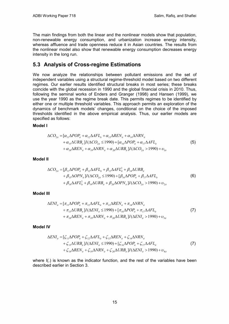
We now analyze the relationships between pollutant emissions and the set of independent variables using a structural regime-threshold model based on two different regimes. Our earlier results identified structural breaks in most series; these breaks coincide with the global recession in 1990 and the global financial crisis in 2010. Thus, following the seminal works of Enders and Granger (1998) and Hansen (1999), we use the year 1990 as the regime break date. This permits regimes to be identified by either one or multiple threshold variables. This approach permits an exploration of the dynamics of benchmark models’ changes, conditional on the choice of the imposed thresholds identified in the above empirical analysis. Thus, our earlier models are specified as follows: Model I

2 11 12 13 14

15 2 16 17

18 19 20 2 1

[ ] ( 1990) [ ] ( 1990)

it it it it it

it it it it

it it it it it

CO POP AFL REN NRNURB I CO POP AFLREN NRN URB I CO

α α α αα α αα α α υ

∆ = ∆ + ∆ + ∆ + ∆+ ∆ ∆ ≤ + ∆ + ∆+ ∆ + ∆ + ∆ ∆ > +

(5)

Model II

22 11 12 13 14

15 2 16 172

18 19 20 2 2

[ ] ( 1990) [

] ( 1990)

it it it it it

it it it it

it it it it it

CO POP AFL AFL URBOPN I CO POP AFL

AFL URB OPN I CO

β β β ββ β β

β β β υ

∆ = ∆ + ∆ + ∆ + ∆+ ∆ ∆ ≤ + ∆ + ∆

+ ∆ + ∆ + ∆ ∆ > +

(6)

Model III

11 12 13 14

15 16 17

18 19 20 3

[ ] ( 1990) [ ] ( 1990)

it it it it it

it it it it

it it it it it

ENI POP AFL REN NRNURB I ENI POP AFLREN NRN URB I ENI

π π π ππ π ππ π π υ

∆ = ∆ + ∆ + ∆ + ∆+ ∆ ∆ ≤ + ∆ + ∆+ ∆ + ∆ + ∆ ∆ > +

(7)

Model IV

11 12 13 14

15 16 17

18 19 20 4

[ ] ( 1990) [ ] ( 1990)

it it it it it

it it it it

it it it it it

ENI POP AFL REN NRNURB I ENI POP AFLREN NRN URB I ENI

ζ ζ ζ ζζ ζ ζζ ζ ζ υ

∆ = ∆ + ∆ + ∆ + ∆+ ∆ ∆ ≤ + ∆ + ∆+ ∆ + ∆ + ∆ ∆ > +

(7)

where I(.) is known as the indicator function, and the rest of the variables have been described earlier in Section 3.

15


The estimated parameters of all the models under both regimes are presented in Table 12. Interestingly, the signs of all the coefficients and their statistical significance remain largely the same under both regimes (before and after 1990) for all variables in both linear and non-linear models. The results indicate that whereas urbanization plays a significant and positive role in increasing emissions in the second regime (Equation 5), openness reduces pollution (Equation 6) in the first regime. With respect to findings related to energy intensity, openness significantly reduces energy intensity in the first regime in Equation (8).

Table 12: Estimates of the Multiple-regime Models 1st Regime 2nd Regime Coefficient t-statistics Coefficient t-statistics

Dependent Variable: Emission Model I a11 0.747 1.13 a16 0.460 0.50 a12 0.501*** 3.52 a17 –0.593** –2.26 a13 –0.103*** –3.51 a18 –0.025 –0.45 a14 0.421*** 8.25 a19 0.126 1.01 a15 –0.124 –0.39 a20 4.461*** 4.82 Model II b11 1.876*** 2.88 b16 1.429 1.20 b12 –15.522** –2.40 b17 –8.124 –0.19 b13 8.129** 2.40 b18 9.204 0.19 b14 0.110 0.36 b19 2.137** 2.34 b15 –0.123*** –3.17 b20 0.011 0.13 Dependent Variable: Energy Intensity Model III c11 –0.299 –0.76 c16 –0.987* –1.82 c12 –0.476*** –5.63 c17 –0.652*** –4.19 c13 –0.026 –1.53 c18 0.050 1.53 c14 0.099*** 3.25 c19 0.081 1.09 c15 –0.146 –0.78 c20 0.863 1.57 Model IV d11 0.032 0.09 d16 –0.897 –1.36 d12 –7.228 –0.48 d17 4.147 0.29 d13 8.405 0.48 d18 –2.387 –0.29 d14 –0.078 –0.47 d19 1.273** 2.51 d15 –0.063*** –2.93 d20 0.081 1.60

Note: (***) indicates that the test statistics are significant at the 1% level, with (**) indicating 5%, and (*) indicating 10%.

5.4 A Further Investigation

In the above, we use panel estimators, like MG, CCEMG, and AMG, considering that the panel is cointegrated as a whole. Although urbanization-pollutant emissions and urbanization-energy intensity are shown to be cointegrated, this is not equivalent to cointegrating relationships existing for each country of the panel. Rejection of null hypothesis of no cointegration in a panel setting could either indicate a cointegrating

16


relationship holds for all cross-sectional units, or that a cointegrating relationship holds for only a small fraction of cross-sectional units (Westerlund et al. 2015). However, it is valid to proceed with panel estimations and inferences in cases of full panel cointegration. Hence, checking the cointegrating property of each country seems essential. If the URB is shown to be cointegrated with pollutant emissions or energy intensity for each country, the results from panel estimation are further credited. Therefore, we resort to applying the autoregressive distributed lag (ARDL)3 bounds testing approach. Tables 13A and 13B present the bounds testing results and the estimated coefficients on URB for all 13 emerging Asian economies. It appears that the cointegrating relationship exists for each economy. It validates the earlier result that the panel is cointegrated as a whole rather than fractional cointegration due to heterogeneity in each economy. These tables also reveal that the estimated error correction term for each economy is negative and statistically significant for both pollutant emissions and energy intensity. However, the speed of adjustment varies considerably, ranging from 1% in India to nearly 96% in Mongolia in the urbanization-pollutant emissions model, as well as from 3% in the PRC to nearly 58% in the Republic of Korea in the urbanization-energy intensity model.4 The columns URB and ∆URB report the estimated long-run and short-run impacts of urbanization on emissions and energy intensity, respectively. The long run results reveal that urbanization significantly increases long-run pollutant emissions in Bangladesh, India, Indonesia, the Republic of Korea, Malaysia, Pakistan, the Philippines, Thailand, and Viet Nam. By contrast, in the long run, urbanization seems to be a vital factor for energy intensity in Bangladesh; the PRC; Hong Kong, China; India; Indonesia; the Republic of Korea; Malaysia; Mongolia; and Pakistan. Interestingly enough, the direction of these long-run impacts in energy intensity are mixed for different countries. This could be influenced by the varying technologies adopted in different countries to cope with increasing energy consumption due to rapid urbanization. As far as short-run causality is concerned, urbanization causes pollution in Hong Kong, China; India; Indonesia; the Republic of Korea; Malaysia; Mongolia; the Philippines, Sri Lanka, Thailand and Viet Nam. Short-run causality from urbanization to energy intensity only runs in Bangladesh; Hong Kong, China; India; Malaysia; Mongolia; Pakistan; the Philippines; and Sri Lanka. These results are consistent with our previous results. Another interesting finding from our time series analyses regarding two Asian giants is that urbanization plays a very active role in increasing pollutant emission and reducing energy intensity in India in both the long and short run, while the impact of urbanization is not so significant in the PRC. The answer may lie in vigorous adoption of cleaner technologies in the PRC, like the recent investment in clean coal and renewables.

3 We do not specify here the unrestricted error correction version for each model and the detail of the ARDL approach to save space. We also presented our key variable, urbanization, in Tables 13A and 13B for the same reason.

4 Three estimated coefficients of ECMt-1 from Pakistan, the Philippines, and Sri Lanka in the urbanization-pollutant emissions model and two from Bangladesh and Pakistan in the urbanization-energy intensity model are larger than one in magnitude, meaning that the economic system is not stable. We suspect this may be due to limited observations.

17


Table 13A: Autoregressive Distributed Lag Bounds Testing to Individual Countries for Pollutant Emissions

Economies Model I

Bounds Testing ECMt-1 URB ∆URB Bangladesh 4.283** –0.520** 1.221** 3.289* The PRC 4.555** –0.310** 0.192 1.735 Hong Kong, China 4.263** –0.471*** 3.051* 2.037 India 4.247** –0.010** 4.049*** 9.428*** Indonesia 4.166** –0.506*** 4.168*** 14.787*** Republic of Korea 2.813** –0.870*** 4.168*** 4.890** Malaysia 5.695** –0.536*** 9.459** 2.901* Mongolia 7.062** –0.956*** 2.185* 5.235** Pakistan 12.103** –1.216*** 3.056*** 1.443 Philippines 10.971** –1.940*** 0.227* 19.574*** Sri Lanka 4.906** –1.311*** 1.577 10.235*** Thailand 6.024** –0.718*** 0.561*** 9.160*** Viet Nam 4.525** –0.814*** 2.100** 8.836***

Economies Model II

Bounds Testing ECMt-1 URB ∆URB Bangladesh 8.424** –0.037** –2.276 0.216 The PRC 4.356** –0.122*** 6.271 0.276 Hong Kong, China 9.676** –0.881*** 2.053 3.836*** India 8.583** –0.384*** 3.522*** 10.912*** Indonesia 10.354** –0.145*** –0.189*** 4.948** Republic of Korea 6.744** –0. 735*** 1.235*** 6.729*** Malaysia 4.513** –0.897*** 7.742*** 5.808** Mongolia 4.071** –0.432*** –4.127 3.642* Pakistan 4.499** –0.089*** 5.207 1.502 Philippines 8.333** –0.387*** 1.457** 10.297*** Sri Lanka 8.174** –0.696*** –0.865 0.191 Thailand 8.767** –0.696*** 1.047*** 13.314*** Viet Nam 4.990** –0.115** –3.202 0.216

Note: PRC = People’s Republic of China. (***) indicates that the test statistics are significant at the 1% level, with (**) indicating 5%, and (*) indicating 10%. Elasticities are given in the long-run analysis while for short-run χ2 values are reported. AIC criterion was adopted for selecting the optimum lag length. t-statistics are in the parentheses for long-run coefficients.

18


Table 13B: Autoregressive Distributed Lag Bounds Testing to Individual Countries for Energy Intensity

Economies Model III

Bounds Testing ECMt-1 URB ∆URB Bangladesh 6.455** –1.257*** 0.015** 2.452 The PRC 4.475*** –0.030*** –0.471 1.571 Hong Kong, China 4.410*** –0.161** –0.288** 4.629** India 10.983*** –0.019** –10.900** 6.993*** Indonesia 5.159*** –0.012** –4.826*** 0.416 Republic of Korea 7.480*** –0.579** 0.240*** 5.043 Malaysia 6.638*** –0.003** –5.719*** 21.043*** Mongolia 7.640** –0.580** 1.748 0.205 Pakistan 10.155** –1.906*** 0.175*** 11.748*** Philippines 5.376** –0.457*** –0.300 0.047 Sri Lanka 7.522** –0.095*** –31.598 12.345*** Thailand 12.678** –0.186*** –1.265 1.344 Viet Nam 4.259** –0.398*** 0.221 0.591

Economies Model IV

Bounds Testing ECMt-1 URB ∆URB Bangladesh 4.200** –0.153*** 1.019** 4.526** The PRC 5.380** –0.459** –4.972** 1.593 Hong Kong, China 4.214** –0.094** –6.766 1.401 India 4.951** –0.319*** –7.464*** 18.796*** Indonesia 4.365** –0.038** 3.270 0.800 Republic of Korea 5.136** –0.167** 0.521 0.718 Malaysia 9.349** –0.881*** 4.971*** 4.948** Mongolia 6.020** –0.881*** 4.436** 4.180** Pakistan 5.241** –0.136*** –4.124 0.688 Philippines 6.504** –0.021** 30.284 5.674** Sri Lanka 7.483** –0.341** –1.648 4.596** Thailand 16.540** –0.228*** –0.043 0.012 Viet Nam 6.725** –0.217*** –4.154 0.925

Note: PRC = People’s Republic of China. (***) indicates that the test statistics are significant at the 1% level, with (**) indicating 5%, and (*) indicating 10%. Elasticities are given in the long–run analysis while for short-run χ2 values are reported. AIC criterion was adopted for selecting the optimum lag length. t-statistics are in the parentheses for long-run coefficients.

19


6. CONCLUSION AND POLICY IMPLICATIONS The objective of this paper is to examine the impact of urbanization on pollutant emissions and energy intensity after controlling for disaggregated energy consumption, trade liberalization, and economic growth in selected emerging Asian economies. We use both linear and nonlinear panel data modeling techniques and employ the recently introduced mean group estimation methods that allow for heterogeneity and cross-sectional dependence. In addition, the relationship between affluence and CO2 emissions is examined in the context of the EKC hypothesis. Moreover, we perform all relevant diagnostic and specification tests that are necessary for obtaining unbiased and consistent regression results. Finally, we use the ARDL model to get country-specific estimates to validate our results from panel estimators. The empirical results reveal that the key determinants of CO2 emissions in Asian countries are population, affluence, and non-renewable energy consumption. Our main variable, that is, urbanization, tends to increase emission; however, the result is not statistically significant. This study also finds evidence of the existence of the EKC hypothesis, implying that when a certain level of economic growth has been achieved, emissions tend to decline. Results from nonlinear estimation show that renewable energy consumption, urbanization, and trade openness reduce emissions. The short-term findings indicate that population, affluence, and both renewable and non-renewable energy consumption have a positive and significant effect on CO2 emissions, implying that these four factors do Granger-cause CO2 emissions. The results from both the linear and the nonlinear models reveal that population and non-renewable energy consumption increase energy intensity while economic growth and trade openness tend to decrease energy intensity. The results also demonstrate that population, affluence, and non-renewable energy consumption have a positive and significant effect on energy intensity, indicating that, in the short run, these three variables Granger-cause energy intensity. However, results from linear and nonlinear estimation show that our key variable, urbanization tends to increase energy intensity in these selected Asian developing countries. This result is contrary to the compact city hypothesis in that energy efficiency improves with urbanization. The above results are also corroborated by country-specific results from the ARDL bound testing approach. The above results have some important policy implications. Reduction of energy usage and pollutant emissions will be possible along with urbanization if governments of these countries do the following: (i) support renewable energy development and encourage construction of renewable energy producing and supplying infrastructure; (ii) develop a highly energy-efficient and emissions-reducing industry base; (iii) encourage a liberal trade regime for clean technology transfer from developed countries; and (iv) promote urbanization with low-carbon urban infrastructure and transportation systems to achieve sustainable growth in these emerging Asian economies.

20


REFERENCES Apergis, N., J. E. Payne, K. Menyah, and Y. Wolde-Rufael. 2010. On the causal

dynamics between emissions, nuclear energy, renewable energy, and economic growth. Ecological Economics 69 (11): 2255–2260.

Banerjee, A. and J. L. Carrion-i-Silvestre. 2013. Cointegration in panel data with structural breaks and cross-section dependence. Journal of Applied Econometrics, DOI: 10.1002/jae.2348.

Bond, S. and M. Eberhardt, 2009. Cross-section dependence in nonstationary panel models: A novel estimator. Paper presented in the Nordic Econometrics Conference in Lund, Sweden.

Boyko, C. T., and R. Cooper 2011. Clarifying and re-conceputalizing density, Prog. Plann, 76, 1–61.

Breitung, J., 2000. The local power of some unit root tests for panel data. Adv. Econometrics 15, 161–178.

Carrión-i-Silvestre, J. L., T. Del Barrio., E. López-Bazo. 2005. Breaking the panels. An application to the GDP per capita. Econometrics J. 8: 159–175.

Chester, M. V. et al. 2014. Positioning infrastructure and technologies for low-carbon urbanization. Earth’s Future.

Cole, M. A., and E. Neumayer. 2004. Examining the Impact of Demographic Factors on Air Pollution. Population & Environment 26(1): 5–21.

Dalton, M., B. O’Neill, A. Prskawetz, L. Jiang, and J. Pitkin. 2008. Population aging and future carbon emissions in the United States, Energy Econ. 30, 642–675.

Dickey, D. A. and W. A. Fuller. 1979. Distribution of estimators for time series regressors with a unit root. Journal of the American Statistical Association 74; 427–431.

Eberhardt, M., and F. Teal. 2010. Productivity analysis in global manufacturing production, Economics Series Working Papers. University of Oxford.

Ehrlich, P. R., and J. P. Holdren 1971. Impact of population growth, Science 171(3977): 1212–1217.

Emirmahmutoglu, F. and T. Omay. 2014. Reexamining the PPP hypothesis: A nonlinear asymmetric heterigeneoud panel unit root test. Economic Modelling 40: 184–190.

Fan, Y., L.-C. Liu, G. Wu, and Y.-M. Wei. 2006. Analyzing impact factors of CO2 emissions using the STIRPAT model. Environmental Impact Assessment Review 26 (4): 377–395.

Frees, E. W. 1995. Assessing cross-sectional correlation in panel data. Journal of Econometrics 69(2): 393–414.

Friedman, M. 1937. The use of ranks to avoid the assumption of normality implicit in the analysis of variance. J. Am. Stat. Assoc. 32: 675–701.

Galeotti, M. and A. Lanza. 1999. Richer and cleaner? A study on carbon dioxide emissions by developing countries. Energy Policy 27: 565–573.

21


Grossman, G. M. and A. B. Krueger. 1993. Environmental impacts of a North American free trade agreement, in Garber, P., ed., The U.S.–Mexico Free Trade Agreement, Cambridge, MA: MIT Press.

Grossman, G. and A. Krueger. 1995. Economic growth and the environment. Halicioglu, F. 2009. An econometric study of CO2 emissions, energy consumption,

income and foreign trade in Turkey. Energy Policy 37(3): 1156–1164. Hamit-Haggar, M. 2012. Greenhouse gas emissions, energy consumption and

economic growth: A panel cointegration analysis from Canadian industrial sector perspective. Energy Economics 34(1): 358–364.

Hossain, M. S. 2011. Panel estimation for CO2 emissions, energy consumption, economic growth, trade openness and urbanization of newly industrialized countries. Energy Policy 39: 6,991–6,999.

Hutyra, L. R. et al. 2014. Urbanization and the carbon cycle: Current capabilities and research outlook from the natural science perspective. Earth’s Future 2(10):473–495.

Im, K., M. H. Pesaran, and Y. Shin. 2003. Testing for unit root in heterogeneous panels. Journal of Econometrics 115: 53–74.

Jones, D. W. 1991. How urbanization affects energy use in developing countries, Energy Policy 19(7): 621–630.

Jones, D. W. 2004. Urbanization and energy. Encyclopedia of Energy 6: 329–335. Kapetanios, G., J. Mitchell, and Y. Shin. 2014. A non-linear panel data model of cross-

section dependence. Journal of Econometrics 179: 134–157. Kasman, A. and Y. S. Duman. 2015. CO2 emissions, economic growth, energy

consumption, trade and urbanization in new EU member and candidate countries: A panel data analysis. Economic Modelling 44: 97–103.

Kearsley, A. and M. Riddel. 2010. A further inquiry into the Pollution Haven Hypothesis and the Environmental Kuznets Curve. Ecological Economics 69: 905–919.

Lariviere, I., and G. Lafrance. 1999. Modelling the electricity consumption of cities: Effect of urban density. Energy Econ. 21(1): 53–66.

Lean, H., and R. Smyth. 2010. CO2 emissions, electricity consumption and output in ASEAN. Applied Energy 87(6):1858–1864.

Levin, A., C.-F. Lin, and C. S. J. Chu. 2002. Unit root tests in panel data: Asymptotic and finite sample properties. Journal of Econometrics 108: 1–24.

Liddle, B. 2014. Impact of population, age structure and urbanization on carbon emissions/energy consumption: Evidence from macro-level, cross-country analyses, Popul. Environ. 35(3): 286–304.

Liddle, B., and S. Lung. 2010. Age-structure, urbanization and climate change in developed countries: Revisiting STIRPAT for disaggregated population and consumption-related environmental impacts, Popul. Environ. 31: 317–343.

Maddala, G. S. and S. Wu. 1999. A Comparative Study of Unit Root Tests with Panel Data and a New Simple Test. Oxford Bulletin of Economics and Statistics 61: 631–52.

22


Madlener, R., and Y. Sunak. 2011. Impacts of urbanization on urban structures and energy demand: What can we learn for urban energy planning and urbanization management? Sustainable Cities and Society 1: 45–53.

Marcotullio, P. J., et al. 2013. The geography of global urban greenhouse gas emissions: An exploratory analysis, Clim. Change 121(4): 621–634.

Martínez-Zarzoso, I., and A. Maruotti. 2011. The impact of urbanization on CO2 emissions: Evidence from developing countries. Ecological Economics 70(7): 1344–1353.

Menyah, K., and Y. Wolde-Rufael. 2010. CO2 emissions, nuclear energy, renewable energy and economic growth in the US. Energy Policy 38(6): 2911–2915.

Menz, T., and H. Welsch. 2012. Population aging and carbon emissions in OECD countries: Accounting for life-cycle and cohorts effects, Energy Econ. 34(3): 842–849.

Midden, C. J. H., F. G. Kaiser, and L. T. McCalley. 2007. Technology’s four roles in understanding individuals’ conservation of natural resources, J. Soc. Issues: 63(1): 155–174.

Newman, P., and J. Kenworthy. 1989. Gasoline consumption and cities: A comparison of U.S. cities with a global survey, J. Am. Plann. Assoc. 55(1): 24–37.

———. 1999. Sustainability and Cities. Washington, DC: Island Press. Oleson, K. W., G. B. Bonan, J. Feddema, and M. Vertenstein. 2008. An urban

parameterization for a global climate model. Part II: Sensitivity to input parameters and the simulated urban heat island in offline simulations, J. Appl. Meteorol. Climatol. 47: 1061–1076.

O’Neill, B. C. 2010. Global demographic trends and future carbon emissions, Proc. Natl. Acad. Sci. U. S. A. 107(41): 17,521–17,526.

Parikh, J., and V. Shukla. 1995. Urbanization, energy use and greenhouse effects in economic development: Results from a cross-national study of developing countries. Global Environmental Change 5(2): 87–103.

Pataki, D. E. et al. 2011. Coupling biogeochemical cycles in urban environments: Ecosystem services, green solutions, and misconceptions, Front. Ecol. 9(11): 27–36.

Pesaran, M. H. 1997. The role of economic theory in modelling the long run. Economic Journal 107: 178–191.

———. 2004. General diagnostic tests for cross section dependence in panels. ———. 2006. Estimation and inference in large heterogeneous panels with a

multifactor error structure. Econometrica 74: 967–1012. Pesaran, M. H., and R. P. Smith. 1995. Estimating long-run relationships from dynamic

heterogeneous panels. Journal of Econometrics 68, 79–113. Philips, P. C. B., and P. Perron. 1988. Testing for a unit root in time series regression.

Biometrika 75: 12. Rafiq, S., R. Salim, and I. Nielsen. 2016. Urbanization, openness, emissions and

energy intensity: A study of increasingly urbanized emerging economies, Energy Economics 56: 20–28.

23


Sadorsky, P. 2009. Renewable energy consumption and income in emerging economies. Energy Policy 37(10): 4021–4028.

———. 2013. Do urbanization and industrialization affect energy intensity in developing countries? Energy Economics 37: 52–59.

———. 2014. The effect of urbanization on CO2 emissions in emerging economies. Energy Economics 41: 147–153.

Salim, R. A., and S. Rafiq. 2012. Why do some emerging economies proactively accelerate the adoption of renewable energy? Energy Economics 34(4): 1051–1057.

Selden, T. M., and D. Song. 1994. Environmental quality and development: Is there a Kuznets curve for air pollution? Environmental Economics and Management 27: 147–162.

Shafiei, S. and Salim, R. A. 2014. Non-renewable and renewable energy consumption and CO2 emissions in OECD countries: A comparative analysis. Energy Policy 66: 547–556.

Sharma, S. S. 2010. Determinants of carbon dioxide emissions: empirical evidence from 69 countries. Applied Energy 88: 376–382.

Soytas, U., R. Sari, and B. T. Ewing. 2007. Energy consumption, income, and carbon emissions in the United States. Ecological Economics 62(3–4):482–489.

United Nations, Population Division, 2015. Department of Economic and Social Affairs. World Urbanization Prospects: The 2014 Revision (ST/ESA/SER.A/366).

Westerlund, J. 2007. Testing for error correction in panel data. Oxford Bulletin of Economics and Statistics 69: 709–748.

Word Bank. 1992. World Development Report: Development and the Environment. York, R., E. A. Rosa, and T. Dietz. 2003. Footprints on the earth: The environmental

consequences of modernity. American Sociological Review 68(2): 279–300.

24

Date post:	04-May-2018
Category:	Documents
Upload:	trantram
View:	221 times
Download:	1 times

Asian Development Bank Institute · adbi working paper series . urbanization, energy consumption,...

Documents