IEEE TRANSACTIONS ON ELECTROMAGNETIC COMPATIBILITY, VOL. EMC-22. NO. 1, FEBRUARY 1980
Aspects of Parallel-Polarized and Cross-Polarized RadarReturns from a Rough Sea Surface
HAROLD R. RAEMER, SENIOR MEMBER, IEEE, AND DOUGLAS D. PREIS, MEMBER, IEEE
Abstract-This paper contains an introductory summary andsimplification of a comprehensive theoretical analysis of radar scatteringfrom a rough sea surface. It includes computed curves which displayreceived signal power integrated over the antenna beam and range gate as afunction of radar geometry. An important feature of the work is thatpolarization is defined with respect to the antenna aperture rather than thesea surface. Because of the finite antenna beamwidth, there is somecross polarization in the radar return which is predictable from first-orderperturbation theory.Key Words-Radar returns, parallel polarized. cross polarized, relative
to aperture plane, rough sea surface.
INTRODUCTIONC ROSS POLARIZATION in a radar return results in a
Corruption of the desired signal. It is an undesired effectlimiting, for a given transmitter, the useful radar coveragedistance, just as receiver noise and interference from mul-tipath propagation or undesired signals limit usable dist-ances of communications systems. It is for this reason thatcross-polarized radar returns are of interest to some EMCengineers.
Cross polarization in a radar return from a rough seasurface [1]-[7] has been observed experimentally. First-order perturbation theory [8] does not predict this pheno-menon. In order to account for observed cross polarizationby perturbation techniques, the usual procedure involvescalculating higher order returns.1 This report is based upon acomprehensive analysis of radar return from a rough seasurface [9]. It contains an introductory summary, a generaltheoretical development, and a useful first-order simplifi-cation of the theory which predicts cross polarization.Various computed curves displaying received signal poweras a function of radar geometry are included. The originalinvestigation was undertaken in an attempt to explain certainexperimental observations on radar returns from targetswhen these returns were corrupted by sea-surface scatter.The present analysis is based upon the perturbation
procedure originally used by Rice [8]; however, this work
Manuscript received August 16, 1979; revised September 17, 1979.H. R. Raemer is with the Department of Electrical Engineering,
Northeastern University, Boston, MA 02115, and the Naval ResearchLaboratory, Washington, DC 20375. (617) 4-37-3035.
D. D. Preis is with the Department of Electrical Engineering, TuftsUniversity, Medford, MA 02115.
1 There are some exceptions to this statement. For example, crosspolarization due to tilt of the reflecting plane was considered by Wright[2] using only first-order theory. However, this arises from a differentmechanism than the "quasi-cross polarization" discussed in the presentpaper.
differs from most previous works [1]-[8] and [10]-[19] intwo respects. First, polarization is defined relative to theradar-antenna aperture plane rather than the sea surface.Secondly, the antenna beamwidth is finite, so that the totalreceived power consists of a superposition (i.e., integrationover the antenna pattern) of fields returned from thoseportions of the sea surface illuminated within the timeinterval of the radar pulse. Thus with polarization definedrelative to the aperture plane of a finite-beamwidth antenna,horizontally polarized and vertically polarized receivedsignals each consist of a combination of componentshorizontally and vertically polarized relative to the seasurface. This cross polarization in the received signal ispredictable from first-order theory and occurs because of theassumed finite antenna beamwidth. It becomes more pro-nounced for greater beamwidths and greater large-scalefluctuations of the sea surface.
DISCUSSION OF ANALYSIS
The present work is limited to first-order-order resultsfrom the general analysis.2 Details of the analysis arepresented in Appendexes I and II. Numerical results arecomputed for the special case of a perfectly horizontal meansurface. The polarization matrix of the received electric-fieldcomponents is
S SVV SVH 1
LSHV SHH -
whose complex elements are
SVV=So{ -A-BBTVH}
SVH= -SoBTvv
SHV=-SOBTHH
SHH = SO{A - BTHV}
(la)
(lb)
2 Second- and higher order results may be important, particularly inthe study of cross-polarization effects. Second-order results have beenconsidered in previouswork [1J, [4J, [6J-[8J . Third- and some fourth-order results have also been obtained by one of the authors [9J, but nonumerical computation on these results has yet been carried out. Thehigher order results are not actually reported in [91, but will be pre-sented in a later NRL report.
IEEE TRANSACTIONS ON ELECTROMAGNETIC COMPATIBILITY, VOL. EMC-22, NO. 1, FEBRUARY 1980
y
-HaaRadar
Beam Center - Surface of Sea
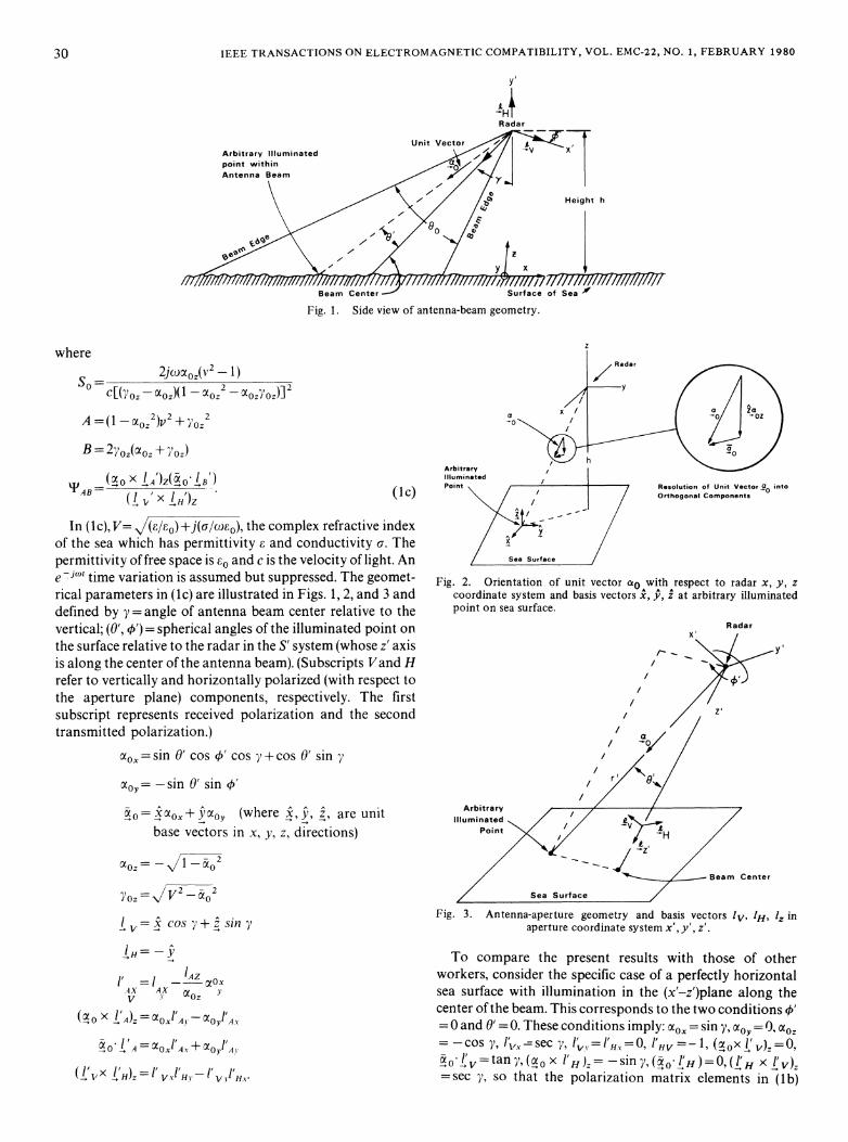
Fig. 1. Side view of antenna-beam geometry.
where
S - 2jcoao.(v2 1)so -CUT(O-aoz)(l- ao.2_X0Z ,0Z)]2
A =(1 - oz )v2 ±yo)
B = 2y0jlo, + ^/Oz)
( X HA)Z(IB)(lv'x(lH'X )z (Ic)
In (Ic),V= (£/co)+j(a/wo), the complex refractive indexof the sea which has permittivity E and conductivity a. Thepermittivity of free space is Eo and c is the velocity of light. Ane Ijw' time variation is assumed but suppressed. The geomet-rical parameters in (1c) are illustrated in Figs. 1, 2, and 3 anddefined by y = angle of antenna beam center relative to thevertical; (O', 4') = spherical angles of the illuminated point onthe surface relative to the radar in the S' system (whose z' axisis along the center of the antenna beam). (Subscripts Vand Hrefer to vertically and horizontally polarized (with respect tothe aperture plane) components, respectively. The firstsubscript represents received polarization and the secondtransmitted polarization.)
aO-=sin 0' cos 4' cos ^y+cos 0' sin y
Xoy=-sin 0' sin O'
+o ox+Y%y (where x, y, z, are unitbase vectors in x, y, z, directions)
YOz- V2 ~2Toz=- l
l =x cos y+L siny
H
I'=I_IAZ loxX AX yOz
(a x )Z=OXAA! Oy'AX
aO IA==oXlAx + OYl A,
(l| x l H)z = l' VxJH -I VvHY
ArbitraryIlluminatedPoint \
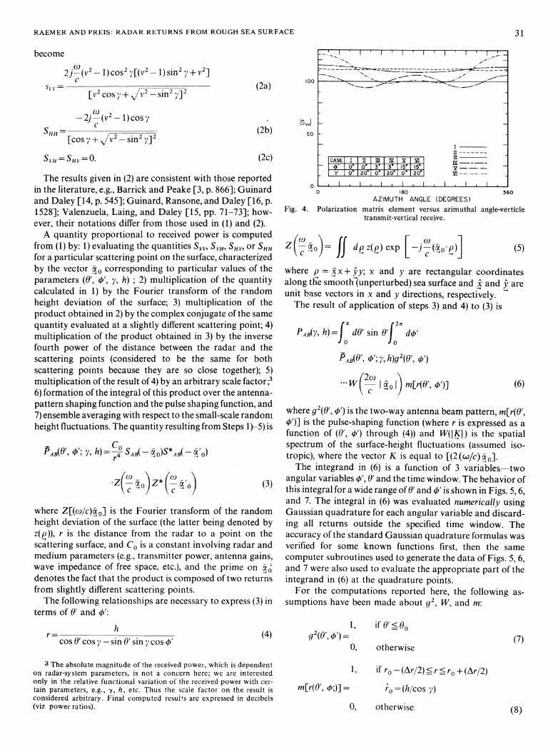
Fig. 2. Orientation of unit vector xo with respect to radar x, y, zcoordinate system and basis vectors x, DP, Z at arbitrary illuminatedpoint on sea surface.
Radar
I--- ~~~~~y
r _ _ y
/ +/ /
// /s
ArbitraryIlluminated
Point
Beam Center
Sea Surface
Fig. 3. Antenna-aperture geometry and basis vectors lv, 1H, lZ inaperture coordinate system x', y', z'.
To compare the present results with those of otherworkers, consider the specific case of a perfectly horizontalsea surface with illumination in the (x'-z')plane along thecenter of the beam. This corresponds to the two conditions 4'=0 and 0' =0. These conditions imply: cxOx = sin ',ao, = 0, xoz= -cos , 11,-sec T', I' ='Hx=0, I'HV = , (a0X I') = ,Ol'v=tan ,(ao X 'H)z -sin 'X0-I'H)O,(I'HX 1V)z
=sec y, so that the polarization matrix elements in (lb)
30
RAEMER AND PREIS: RADAR RETURNS FROM ROUGH SEA SURFACE
become
2j C (V2_1) COS2 [(V2 _ 1) sin2 y + V2]~~~~II=~~~~~~~~~~c t. .--VOS~,++/V2 *-sin2 j2
2~~~~~~~~~
-2j (v -1)cosySHH= 2
= [COS 0t+_.22 _ sin2 j2
S VH =' SHV-= °-
00 180 360
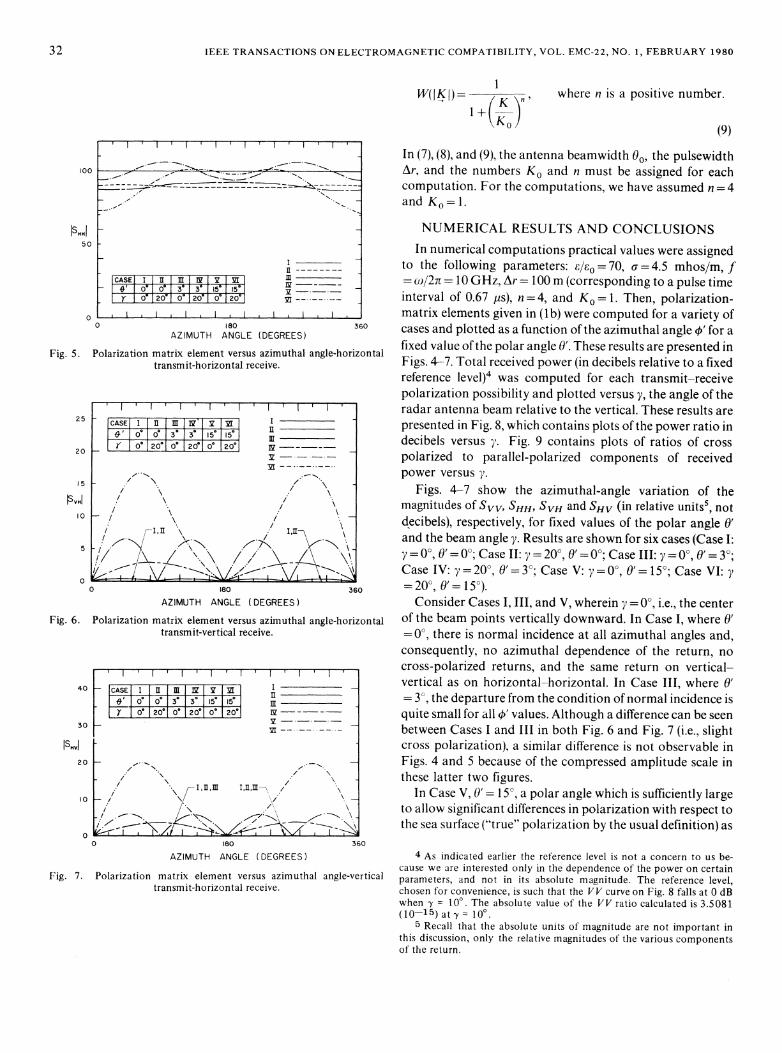
AZIMUTH ANGLE (DEGREES)Fig. 4. Polarization matrix element versus azimuthal angle-verticle
transmit-vertical receive.
Z(w0)=ifoc dp z(e) exp (5)
where p = xx + yy; x and y are rectangular coordinatesalong tfie smooth(unperturbed) sea surface and x and y areunit base vectors in x and y directions, respectively.The result of application of steps 3) and 4) to (3) is
PAB(Y, h) dO' sin O'f d+'
PAB(O, O); 7, h)g , )
(6)
where g2(O', 4') is the two-way antenna beam pattern, m[r(O',4')] is the pulse-shaping function (where r is expressed as afunction of (0', 4') through (4)) and W(IKI) is the spatialspectrum of the surface-height fluctuations (assumed iso-tropic), where the vector K is equal to [(2 (o/c)o 0].The integrand in (6) is a function of 3 variables two
angular variables 4', 0' and the time window. The behavior ofthis integral for a wide range of 0' and 4/ is shown in Figs. 5,6,and 7. The integral in (6) was evaluated numerically usingGaussian quadrature for each angular variable and discard-ing all returns outside the specified time window. Theaccuracy of the standard Gaussian quadrature formulas wasverified for some known functions first, then the samecomputer subroutines used to generate the data of Figs. 5, 6,and 7 were also used to evaluate the appropriate part of theintegrand in (6) at the quadrature points.For the computations reported here, the following as-
sumptions have been made about g2, W, and m:
100(2a)
(2b)JSvvl
50
(2c)
The results given in (2) are consistent with those reportedin the literature, e.g., Barrick and Peake [3, p. 866]; Guinardand Daley [14, p. 545]; Guinard, Ransone, and Daley [16, p.1528]; Valenzuela, Laing, and Daley [15, pp. 71-73]; how-ever, their notations differ from those used in (1) and (2).A quantity proportional to received power is computed
from (1) by: 1) evaluating the quantities Sn,, SVH, SHV, or SHHfor a particular scattering point on the surface, characterizedby the vector -a corresponding to particular values of theparameters (0', 4', y, h) ; 2) multiplication of the quantitycalculated in 1) by the Fourier transform of the randomheight deviation of the surface, 3) multiplication of theproduct obtained in 2) by the complex conjugate of the samequantity evaluated at a slightly different scattering point; 4)multiplication of the product obtained in 3) by the inversefourth power of the distance between the radar and thescattering points (considered to be the same for bothscattering points because they are so close together); 5)multiplication of the result of 4) by an arbitrary scale factor ;36) formation of the integral of this product over the antenna-pattern shaping function and the pulse shaping function, and7) ensemble averaging with respect to the small-scale randonmheight fluctuations. The quantity resulting from Steps 1)-5) is
PAB(O, 4/; r,h= C4 SAB( -O)S AB( --O)
(c -° (c ocO(3
where Z[(w_o/c)aO] is the Fourier transform of the randomheight deviation of the surface (the latter being denoted byz(p)), r is the distance from the radar to a point on thescattering surface, and CO is a constant involving radar andmedium parameters (e.g., transmitter power, antenna gains,wave impedance of free space, etc.), and the prime on osdenotes the fact that the product is composed of two returnsfrom slightly different scattering points.The following relationships are necessary to express (3) in
terms of 0' and 4':
hcos 0' cos y- sin 0' sin , cos 4'
3 The absolute magnitude of the received power, which is dependenton radar-system parameters, is -not a concern here; we are interestedonly in the relative functional variation of the received power with cer-tain parameters, e.g., y, h, etc. Thus the scale factor on the result isconsidered arbitrary. Final computed results are expressed in decibels-(viz power ratios).
1, if 0' <00(4) g2(0',4/,) =
0, otherwise
CASE I |m IM IZ-' o
3 3- 515' 5'0020o1o020e0 20 M
, .
(7)
1, if ro-(Ar/2) _ r _ ro + (Ar/2)
m[r(0', 40;)] =
0, otherwise (8)
31
...w m[r(O', o')].o
f
ro = (h/cos /)
IEEE TRANSACTIONS ON ELECTROMAGNETIC COMPATIBILITY, VOL. EMC-22, NO. 1, FEBRUARY 1980
1
1W±(K )fl=where n is a positive number.
-- -------
II
mv ..
CASE |I II M 7m la lOf 0.3M3vl1nU5' 15°'
o |- 20 |l I 2oe eio°2I I .1 I1 1-
0 180 360AZIMUTH ANGLE (DEGREES)
Fig. 5. Polarization matrix element versus azimuthal angle-horizontaltransmit-horizontal receive.
lI25 CASE I II Mm m I_
O'e°0 3° 3° 15' 15 m
DI
20 _ 0° 20° °20°j0° l m- - -
00 180 360
AZIMUTH ANGLE (DEGREES)
Fig. 6. Polarization matrix element versus azimuthal angle-horizontaltransmit-vertical receive.
I -l I I I I
CASE I II I|' e j0° 3° 3°15010er eo 20° o° 20° o°* 20°
T I
II
Il
m30 M-
/'.
N
I/0
,.1
I/'1,11,11 i,n1,m111 \
180
\
(9)
In (7), (8), and (9), the antenna beamwidth 00, the pulsewidthAr, and the numbers Ko and n must be assigned for eachcomputation. For the computations, we have assumed n = 4and Ko = 1.
NUMERICAL RESULTS AND CONCLUSIONSIn numerical computations practical values were assigned
to the following parameters: E/&0= 70, a = 4.5 mhos/m, f=O/2r=210 GHz, Ar = 100 m (corresponding to a pulse timeinterval of 0.67 [us), n= 4, and Ko= 1. Then, polarization-matrix elements given in (lb) were computed for a variety ofcases and plotted as a function of the azimuthal angle p' for afixed value of the polar angle 0'. These results are presented inFigs. 4-7. Total received power (in decibels relative to a fixedreference level)4 was computed for each transmit-receivepolarization possibility and plotted versus y, the angle of theradar antenna beam relative to the vertical. These results arepresented in Fig. 8, which contains plots of the power ratio indecibels versus y. Fig. 9 contains plots of ratios of crosspolarized to parallel-polarized components of receivedpower versus y.
Figs. 4-7 show the azimuthal-angle variation of themagnitudes of Svv, SHII, SVH and SHV (in relative units5, notdecibels), respectively, for fixed values of the polar angle 0'and the beam angle y. Results are shown for six cases (Case I:y0 ,0'= 0°; Case II: y=20°, 0'= 0°; Case III: y =0°, 0'=3;Case IV: y=20, 0'=3; Case V: y =O°, 0'= 15°; Case VI: y=20°, 0'=15).Consider Cases I, III, and V, wherein y = 0°, i.e., the center
of the beam points vertically downward. In Case I, where 0'=0°, there is normal incidence at all azimuthal angles and,consequently, no azimuthal dependence of the return, nocross-polarized returns, and the same return on vertical-vertical as on horizontal-horizontal. In Case III, where 0'= 3, the departure from the condition of normal incidence isquite small for all ' values. Although a difference can be seenbetween Cases I and III in both Fig. 6 and Fig. 7 (i.e., slightcross polarization), a similar difference is not observable inFigs. 4 and 5 because of the compressed amplitude scale inthese latter two figures.
In Case V, 0'= 15°, a polar angle which is sufficiently largeto allow significant differences in polarization with respect tothe sea surface ("true" polarization by the usual definition) as
360
AZIMUTH ANGLE (DEGREES)
Fig. 7. Polarization matrix element versus azimuthal angle-verticaltransmit-horizontal receive.
4 As indicated earlier the reference level is not a concern to us be-cause we are interested only in the dependence of the power on certainparameters, and not in its absolute magnitude. The reference level,chosen for convenience, is such that the VV curve on Fig. 8 falls at 0 dBwhen -Y = 100. The absolute value of the VV ratio calculated is 3.5081(10 -15) at y = 100.
5 Recall that the absolute units of magnitude are not important inthis discussion, only the relative magnitudes of the various componentsof the return.
32
,00
ISNHH50
0
40
ISHVI20
10
0
RAEMER AND PREIS: RADAR RETURNS FROM ROUGH SEA SURFACE
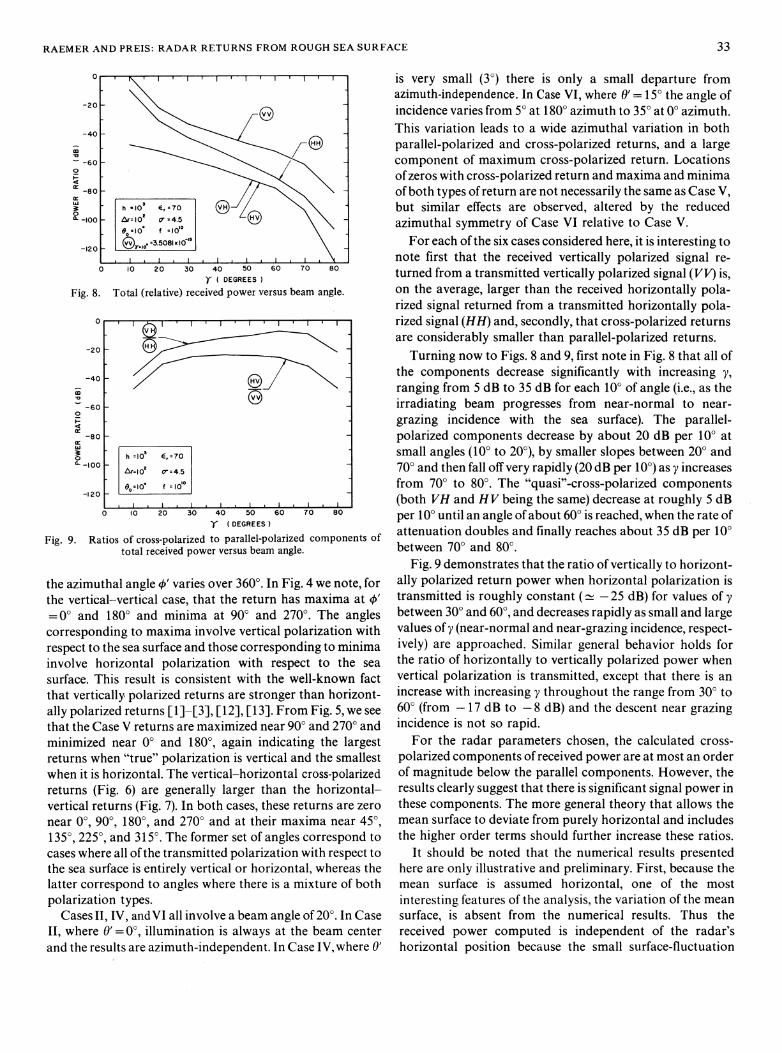
r ( DEGREES,Fig. 8. Total (relative) received power versus beam angle.
r (DEGREES)
Fig. 9. Ratios of cross-polarized to parallel-polarized components oftotal received power versus beam angle.
the azimuthal angle P' varies over 3600. In Fig. 4 we note, forthe vertical-vertical case, that the return has maxima at 4'= 00 and 1800 and minima at 900 and 270°. The anglescorresponding to maxima involve vertical polarization withrespect to the sea surface and those corresponding to minimainvolve horizontal polarization with respect to the sea
surface. This result is consistent with the well-known factthat vertically polarized returns are stronger than horizont-ally polarized returns [1]-[3], [12], [13]. From Fig. 5, we see
that the Case V returns are maximized near 900 and 2700 andminimized near 00 and 1800, again indicating the largestreturns when "true" polarization is vertical and the smallestwhen it is horizontal. The vertical-horizontal cross-polarizedreturns (Fig. 6) are generally larger than the horizontal-vertical returns (Fig. 7). In both cases, these returns are zero
near 0°, 900, 1800, and 2700 and at their maxima near 45°,1350, 225°, and 3150. The former set of angles correspond tocases where all of the transmitted polarization with respect tothe sea surface is entirely vertical or horizontal, whereas thelatter correspond to angles where there is a mixture of bothpolarization types.
Cases II, IV, andVI all involve a beam angle of 200. In CaseII, where 0'= 00, illumination is always at the beam centerand the results are azimuth-independent. In Case IV, where 0'
is very small (30) there is only a small departure fromazimuth-independence. In Case VI, where 0'= 15' the angle ofincidence varies from 50 at 1800 azimuth to 350 at 00 azimuth.This variation leads to a wide azimuthal variation in bothparallel-polarized and cross-polarized returns, and a largecomponent of maximum cross-polarized return. Locationsofzeros with cross-polarized return and maxima and minimaofboth types of return are not necessarily the same as Case V,but similar effects are observed, altered by the reducedazimuthal symmetry of Case VI relative to Case V.
For each of the six cases considered here, it is interesting tonote first that the received vertically polarized signal re-turned from a transmitted vertically polarized signal (VV) is,on the average, larger than the received horizontally pola-rized signal returned from a transmitted horizontally pola-rized signal (HH) and, secondly, that cross-polarized returnsare considerably smaller than parallel-polarized returns.
Turning now to Figs. 8 and 9, first note in Fig. 8 that all ofthe components decrease significantly with increasing y,ranging from 5 dB to 35 dB for each 100 of angle (i.e., as theirradiating beam progresses from near-normal to near-grazing incidence with the sea surface). The parallel-polarized components decrease by about 20 dB per 100 atsmall angles (10° to 200), by smaller slopes between 20° and70° and then fall off very rapidly (20 dB per 100) as y increasesfrom 700 to 800. The "quasi"-cross-polarized components(both VH and HV being the same) decrease at roughly 5 dBper 100 until an angle of about 600 is reached, when the rate ofattenuation doubles and finally reaches about 35 dB per 100between 70° and 800.
Fig. 9 demonstrates that the ratio of vertically to horizont-ally polarized return power when horizontal polarization istransmitted is roughly constant (- -25 dB) for values of ybetween 30° and 600, and decreases rapidly as small and largevalues of y (near-normal and near-grazing incidence, respect-ively) are approached. Similar general behavior holds forthe ratio of horizontally to vertically polarized power whenvertical polarization is transmitted, except that there is anincrease with increasing y throughout the range from 30° to60° (from - 17 dB to -8 dB) and the descent near grazingincidence is not so rapid.
For the radar parameters chosen, the calculated cross-polarized components of received power are at most an orderof magnitude below the parallel components. However, theresults clearly suggest that there is significant signal power inthese components. The more general theory that allows themean surface to deviate from purely horizontal and includesthe higher order terms should further increase these ratios.
It should be noted that the numerical results presentedhere are only illustrative and preliminary. First, because themean surface is assumed horizontal, one of the mostinteresting features of the analysis, the variation of the meansurface, is absent from the numerical results. Thus thereceived power computed is independent of the radar'shorizontal position because the small surface-fluctuation
33
IEEE TRANSACTIONS ON ELECTROMAGNETIC COMPATIBILITY, VOL. EMC-22, NO. 1, FEBRUARY 1980
statistics are assumed uniform along the surface. A moreinteresting set of results, attainable when the mean surfacevariation is accounted for, would be a trace of the return versustime as an airborne radar traveled along its path illuminatingthe sea surface. This is a subject currently underinvestigation.
Secondly, because of the flat-mean-surface assumption,the cross polarization here is small (as indicated in Figs. 8 and9 where the VH and HV components are between 20 and 40dB below the VV and HH components, respectively). Theeffect would be much more pronounced with a variable meansurface and would increase with increasing mean surfaceamplitude.
Finally, the absence of second- and higher order termseliminates additional cross polarization.6 This consider-ation suggested that the total amount of cross polarizationmay be somewhat greater than predicted here.
APPENDIX I
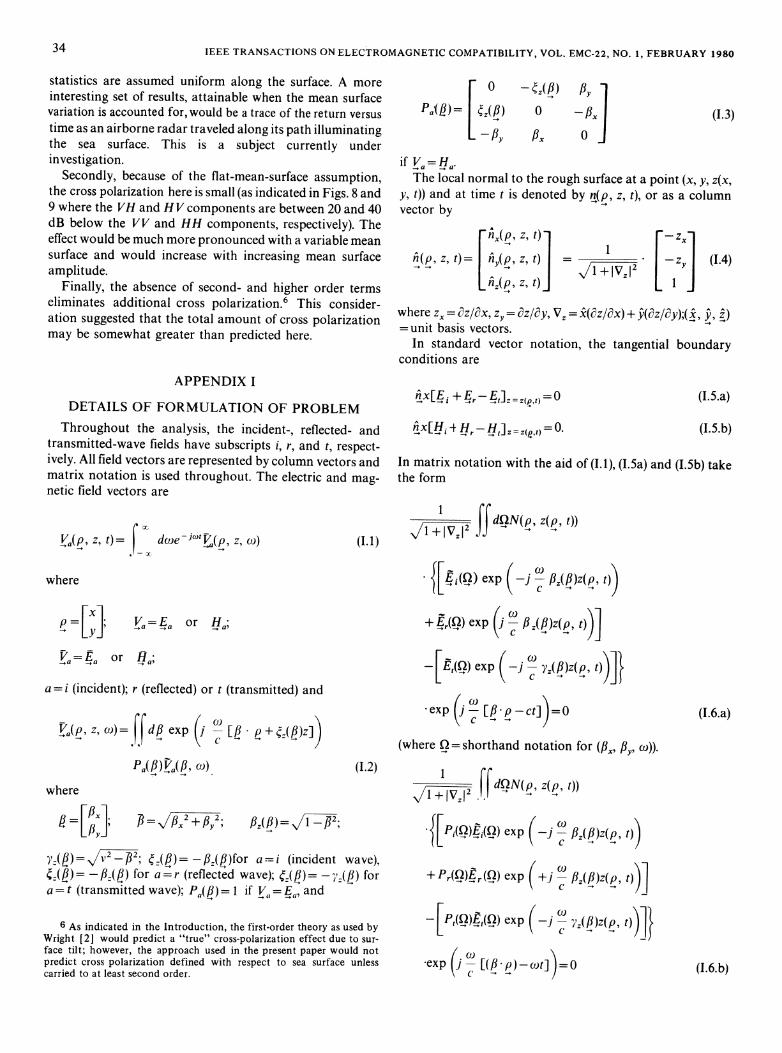
DETAILS OF FORMULATION OF PROBLEMThroughout the analysis, the incident-, reflected- and
transmitted-wave fields have subscripts i, r, and t, respect-ively. All field vectors are represented by column vectors andmatrix notation is used throughout. The electric and mag-netic field vectors are
C-Xwhr(P, Z, t)e= dwe iWtV(P Z, (0)
where
0
Pa(L!P (:(#
fly
- z(fl) Xly0 -Ax
flx O
if Va=H .The local normal to the rough surface at a point (x, y, z(x,
y, t)) and at time t is denoted by n(p, z, t), or as a columnvector by
p,z, t) Zx]
n z, t)= niy(p, z,t)-=1
where zx = ez/ax, z, = 8z/8y, Vz = k(az/ax) + 5(az/ay);(x,', z )=unit basis vectors.
In standard vector notation, the tangential boundaryconditions are
nfx[Ei+Er-Et]z=z(pt) =0
flX[Hi4H,rH1] z = z(p,t) =0.
In matrix notation with the aid of (1.1), (I.5a) and (I.5b) takethe form
1 dQN(p, z(p, t))
+RjQ) exp
(i cofz(#)z(p,t))
[Et(Q) exp (-ic #()Z(-P' ))]
(1.1)
Va=Ea or Ha;
V =Ea or Ha,a = i (incident); r (reflected) or t (transmitted) and
l'a(P Z, w)= FFdJ3 exp ( [/ e +P± )z])
Pawhra(e, (0)
where
(1.2)
p= I/-~Q+f4,T;y (8)= /v2- 2; #z/g)=- f4)for a--i (incident wave),' (i#)= -L,(/) for a=r (reflected wave); r(f)=->(/) fora = t (transmitted wave); Pa(#)-= 1 if Va= E,, and
6 As indicated in the Introduction, the first-order theory as used byWright [21 would predict a "true" cross-polarization effect due to sur-face tilt; however, the approach used in the present paper would notpredict cross polarization defined with respect to sea surface unlesscarried to at least second order.
*exp (- [# p-Ct])=0
(where Q=shorthand notation for ( fy o)).1~~~~~~~~~~~~
<1 ((zdQN(p, z(p, t))
*[Pj(Q)Ej(f2) exp(jzB)p )
+Pr(Q)Er2 exp (+j c fz(#i)Z(P, t))
~~~~~-[P(Q)E(Q) exp (cZP, t))]
*exp (X [(h?p )-c )t] = 0
(1.3)
(1.4)
(I.5.a)
(I.5.b)
(I.6.a)
(I.6.b)
34
#,( # ) = I #2;
xp =--+ -Y-
flxfi= fly-
RAEMER AND PREIS: RADAR RETURNS FROM ROUGH SEA SURFACE
whereO -1I - zy,
N(p, z, t)= [0 zx
LZY -zx °
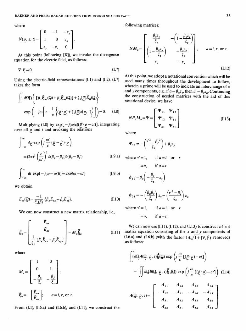
At this point (following [8]), we invoke the divergenceequation for the electric field, as follows:
V E=0. (1.7)
Using the electric-field representations (1.1) and (1.2), (1.7)takes the form
jf' dQU}{ [flxPax(9) + flyEay(Q)] + Uz(I3)Eiz(Q)j
*exp (-jO t-c {(f3.P)+ (f)z(p, t)}])=o . (1.8)
Multiplying (1.8) by exp [-j(w/c)(#'- p -ct)], integratingover all p and t and invoking the reTations
dp exp (j-( P' p
=(27)2 (k) (- fl,)6(f - f3y') (I.9.a)
£ dt exp( -j(co - ')t) = 2rb(o- wo') (I.9.b)
we obtain
following matrices:
NMa = I1 _ PxZx fl_yzx I
zy -zx-
a= i, r, or t.
(1.12)
At this point, we adopt a notational convention which will beused many times throughout the development to follow,wherein a prime will be used to indicate an interchange of xand y components, e.g., if a = f3 ,zy, then a' = f3yz,. Continuingthe construction of needed matrices with the aid of thisnotational device, we have
11 1
NPaMaP=T=[ 2T 11J
331 31 _where
T11=-( + pyzy
where v'= 1,
(1.13)
if a= i or r
=iV, ifa=t
*12=#X fly _zy)
Eaz(Q) = ( {fxEax+ yEay}. (I.1
We can now construct a new matrix relationship, i.e.,
EaxE
Ea Eay J MaEa (I.1
[lfxfax + fy4ay]
where
Ma 0 1a
x p
_X fl
z(Z Z-
0o) 31 = - (fll) Zay- ( I) Z,
where v'=1, if a=i or r
=v, if a=t.
We can now use (I.11), (I.12), and (I.13) to construct a 4 x 41) matrix equation consisting of the x and y components of
(I.6.a) and (I.6.b) (with the factor 1/(1/l+IVI2) removed)as follows:
ffdQA(Q, p, t)E(Q) exp - [(fl P) -ct)
= {fdQB(Q, p, t)E1(Q) exp (j [(f,Bp)-ct]) (1.14)
IEax .+a EL a=i, r, or t.
From (1.1), (I.6.a) and (I.6.b), and (I.11), we construct the
All
A(Q, p, t) = A12
L At32
Al2 A13 A14 1
I' 1 -A14 -
A32 A33 A34
A'31 Al34 At33
35
IEEE TRANSACTIONS ON ELECTROMAGNETIC COMPATIBILITY, VOL. EMC-22, NO. 1, FEBRUARY 1980
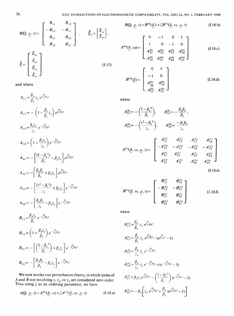
B(Q, p, t)=
B11
- Bfl 2
B3I
L B'
B12
B3 2
Bt3
E'E
Erx
A Ery (1.15)
and where
A=1- zi--
B(Q, p, t) = BI °)(f ) +'B(1)09 CI@,p, t)
0O -1 0 1
A~0~(fl I)= 0 -1 0A(°) A(°1 A(°) A()-
[01-1 0
A(°) A(°)31 32A0) A(O'
where
A(°) (1=/- 2)
(v2- #Y2)Al3= e- c zzo'Z
A (1 Afyzy) _ j6O z
A3 1 =-[ -# Z1 e- L 1ZZ
-A(')'1 2
A('l)
LA(l1)f
A(O =- Mx:Y7z
Al' I(#, (o, p, t)=
A3 2 =[z3-7jZ + xZyj e c
Lv27_ Y2)
LA< __ xz ] e- zz'I/
BI=Ie'JcIezZ
B12 ( Iz+ ) JIe z
31 [-L(' 2z ) +/3yzyj e
B -S # z-)j| e Ji Zz
BII(#, a), p, t)=
B(l1) B(l-B(l)' -B(l )'
12 1 1
B(1) B(3' )31 32
B(1' B(l)'
where
(
#X
Vill ZY. e z
A(1) Ye c z-z (e cY 1)
1 #Z
We now invoke our perturbation theory, in which terms ofA and B not involving z, z, or zy are considered zero order.Thus using ; as an ordering parameter, we have
(z)
A 31 = /SzZ e t'a( ' 2) (ei( )
(I. 16.a) A~(')= -/fx [z, e cfi + (eJcfiz--1)
(I.16.b)
(I.16.c)
(I.16.d)
A"114-A(l)f
A(')34A(')' I33
(I. I 6.e)
(1.16.)
36
fly 0)
z i-#,zAl 2 -": -I -#Z y e c A(O) = MY3 2 #Z 9
A(Q, o, t) = Alo)(fl, o-)) + CA(')(fl, oi, p, t)
37RAEMER AND PREIS: RADAR RETURNS FROM ROUGH SEA SURFACE
o V2 R 2 coA~1~--/3 z eJczz I" I (-,Yzz~lA('l) = Ryye-iCZ _ y (e- cY-)
A343 flSxzy e Tz-,eiZ--)
o (oA('l) = x zy e - czZ+(e- c _1)
34~ yy7
/3(0li-liz Pz
B(3ll) - y e-icfzz+(ei)cPzz
B(1-) -/3yzez c z_Y (eizc )31 yy /z~F (0 / co 1
B('=/3 z~ei cPzZ -(e-JJ#zz -1L2 /3 I
Expanding E in a perturbation series,
Solution of (I.19.0) yields
(1.20.0)
where
k10 (/3, w,)=[-[A)(/3, wo)] -'Bl)(/3, w))and the inverse of A(1) is given by
[A(O (f, wt))] - '= bo(fl)= (/ + y)¢1 - /32 + z
- bll
bil--b'32
bl2 bl3 b14
-b 1 b14 b'l3b32 b13 b14
-b11 b14 b'13where
I(1.17) b 1=-/-/x3y(#z/-vz)
and employing (I.16.a), (I.16.b), and (1.17) in (1.14), we can
In the general analysis, terms of order 2, 3 and beyondwere included. In this paper, consideration is limited to thefirst-order case; hence we will make no further mention ofterms beyond first order in the perturbation series.
Multiplication of (1.18) by exp (-j(w/c)[(/'- p) -ct] andintegration of product on p and t from - xc to + oc, with theaid of (I.9.a) and (I.9.b) yields the following set of perturb-ation equations (after interchanging (#', a') and (/3, w) and
-A(1 (31, wv; , tt A B/31, cw)] 'B' 1(/3l, Cl1)}.The vector E is not of direct use to us. It would be
preferable to have the reflected-wave vector Er To obtain Er'we invoke (I.11) and note that
~rMr [(r -i1' 0[E
=Q(/3)L (1.21)1%
I = Q([3)E (1.21)
IEEE TRANSACTIONS ON ELECTROMAGNETIC COMPATIBILITY, VOL. EMC-22, NO. 1, FEBRUARY 1980
where0 0 0
0 1 0 0
QqQ= [(:x) _(;Y) 0 01The unit vectors corresponding to horizontal and vertical
polarization are given in Appendix II (II.25.a,b) and aredenoted by (v and LH, respectively. The specialized meaningof horizontal and vertical polarization in this paper, differentfrom the standard meaning, is explained in the introductorysection of the paper.The vertically and horizontally polarized components of
E are denoted byTE (.2aErv lvr (I.22.a)
ErH=IEr (I.22.b)
We now relate Ei to Eiv and EiH, the vertically andhorizontally polarized components of the incident-wavevector Ei. From (1.11),
Ei(#) =4#)Ej(4)where
E# EiH(#)-L (18)( VY'I|H ;'-HxtlV)l ) [IHX I V '
IHx,), Vx,y lHx,y, Vx,y + Vz YXY
The remaining analysis, detailed in Appendix II, resfirst-order expressions for vertically and horizontallyrized electric-field components at the receiving point,either vertically or horizontally polarized transmitted
and where b(fl) is the 4x4 matrix given in (1.20.0); A(I/3i)=(fz+±Yz(1_- l2+z+,'y), and a(#, kl) is a 4x2 matrixdefined by
(11.2)
where Bo(# 1) is obtained from (I.16.c) and (I.16.d) with # setto / 1, and the elements of the 4 x 4 matrix A1((g, k 1) and the4X2 matrix B1(g, k 1) are obtained from (I.16.e) and (I.16.f),respectively. The latter elements are the first-order terms ofthe series expansion of (I.16.e) and (I.16.f). The first-orderterms (I.16.e,f) are as follows:
CALCULATION OF FIRST-ORDER RESULTSTo obtain the results from which (laH)Ilc) are obtained, we
first specialize to the case where z(y, t) does not varysignificantly with time during the period of illumination;hence, we can denote z(p, t) by z(e) and its Fourier transformby Z(k), having eliminated by this specialization the necess-ity of Fourier transforming with respect to time as well as thespatial variables.From (1.20.1) (with the assumption indicated above),
E(I)(#, co)-= FdF dddp I dt
*exp [(J(Oil#I- f)O el -c()l -coftl])
To obtain the first-order results, we follow the analysisusing (I.19.0,1), (1.20.0,1), (1.21), (I.22.a), (I.22.b), and (1.23)with the aid of (1.20.0). Expressing z(p), zA(p), and zy(p) interms of their Fourier transforms, we have
Z(P) = FFdk exp ( jk p)Z(k)
: (p) = {FdikX exp (jk p)Z(k)
zy(p) = FFdkjk exp (jk p)Z(k).
(II.4.a)
(II.4.b)
(II.4.c)
(11.1) From (II.4.a)-(II.4.c) and (II.3.a), the element A l could be
38
a(., k 1) = F3, (fl, k 1) i I (fl, k ) bQ# 1) B-+ _, -+ __., -+I A(I # 1 1) OQ# 1)
-A"I(fl, 041, (01, Pj. tl)Ei(,fll, oil)
RAEMER AND PREIS: RADAR RETURNS FROM ROUGH SEA SURFACE
From (11.1), (11.8), and (1.23)
Fdk exp (jk )Z(k)(A11((, k)) (11.5)
where
(AI J# -,k)jk7, flz,k))lkJ
The elements of (Ajk), and (Bjk)l, obtained from (II.3.a)-(II.3.h), as indicated in (11.5), are as follows:
(A 1 l(8, k 1))I =(B1-(3, k )) =i/kJ3 (II.6.a)(A20g k ) =((312(g, k 1)),
=jflyk1 yfz - 1-j cZ (II.6.b)
(A1 3(i, 1)X =jf3Xk1y (II.6.c'
(A14(, k 1))1 =jflykyIY -J
(A31(, k1))h =-(B31(k, 1))X
=jfyk 1y-j - (1f_y2)C
(A32(3, k)) -(A32(1 kl))h
=-jfkxk1y-i C pfJ
(A33(fl, k1))1 =-j/3yk1y+j-(v2 _ i2)
C
(A34Xfl, k!1)) =jflxkl1 +j
(II.6.d)
(II.6.e)
(11.6.0
(II.6.g)
(II.6.h)
The other elements of A and are obtained through therelationships implied by (I.15), i.e.,
A21 = A12 A22 =-A1 A23-=-A4 A24 A13
A41 A32 A42A 31 A43 A34 A44 A33
B21=-B' B22=-B,1' B4,=B3 B42 =B3;1
[ErLH(r4)]1 = d/I [31 (/; # 1)] 1 Ei(i 1)
where
[ ,H(fl; # 1)]1 = IT,HQ(#)bo(il)(a)L ()
(11.9)
(II.10)
and where (a) is the quantity a(f, k ) defined in (11.2).Examining the definition of a(#, k) in (11.2), we note the
matrix product (A1(f; kI)b (l1)), which is a 4x4 matrix.The first step is the calculation of that product. Calling thismatrix product J, using c (not to be confused with the free-space velocity of light) to denote the matrix A-,, and invoking(II.3.a)II.3.h), (II.6.a)-(II.6.h), and (11.7), we obtain
Cl1
1 -C Id=-I 1
A C31
C32
C12 C13 C14
IC -1 4 -C13
C32 C33 C34
C31 C34 C33'
- b1l bl2 bl3 b14
-b2 -1 1 14 bl3
b1l b32 b13 b14-b32 -b11 b14 b13
_ j,jk]A A
(11.11)
wherel[JJjkl=jJ=dA, A is A(1131) as defined above (11.2) and,because of the special properties of the matrices c and b, wehave (note that b1I=b1, b1I=b14)
where the prime indicates that x and y components are
interchanged in the corresponding original element, e.g., ifAjk=XklY, then Ajk-=fikklx.We now invoke (1.21), (I.22.a,b), and (1.23), with the aid of
which we can use (11.1) to express the horizontally andvertically polarized components of the electric field of thereflected wave to the first order of perturbation. The result ofthis operation is
[ELrl,H(f3)] = IL,HQ(#)[E(l)] I (11.8)
where I [H=transpose of 1L,Hl Q(f#) is given in (1.21), andA A
[E(/3)]I is the first-order term of E(f3, w) as given by (11.1).
From (11.13), (11.14), and (11.15), we obtain after considerablemanipulation (again explicitly indicating function
RAEMER AND PREIS: RADAR RETURNS FROM ROUGH SEA SURFACE
arguments)
ajk(/3 k) A(iyjIaJk(f,# k)
a4 I (fl, k)==-fy Ial)kx + a3 lb(I #j)x(11.17)
where
all1(#, k) =611.l(l # tk
+ C al lb(Il I)DxPyC
a2 1(/, k) =a2ia(IpI )kxflx
To specialize the results to the backscattering case, we firstnote that the unit vector ao is defined as that directed fromthe radaL to the illuminated patch. In vector-matrix notation
FOoxl
_OX = CaoyL-Oo= _
(II.20.a)
where
+ [a2lb(Iy)lX2 + a2 lc(l y1
We now define a two-dimensional unit vector aO, theprojection of ao on the x-y plane, as follows:
For backscattering of an incident plane wave or plane-wave pulse, the unit vector corresponding to the direction ofthe incident wave is + xo, while the unit vector correspond-ing to the direction of the back-scattered wave is is -ao.Then
1y =]OX
= [O
(11.18)
Using the above results, we can write (11.18) more
compactly as follows:
ajk(1, k)= A(i,31) aJk(#, k) (II.19)
where
all1(#, k) =#fx {a lal )kY + Cal lb(i # M)y}
621(fl, k)= - x[til (,, k)] + c a2 lc(lt )
a3l(, k) =- [4(, k)] + Co
1(181
flla4J# t3lcC
a3l(, -+ _+ -+ ~C ,1
Continuing the specialization in the backscattering case,we invoke (11.21) and (11.22) in the expression (II.10),resulting in an expression of the form
[Err,H( --a, 0)] I = [S,,H(- a 0; a )]JEj(aO)Z (- c (.)
(11.23)
To continue further the specialization to backscattering,we invoke (11.21) and (11.22) in the expression (11.8) and carryout the matrix operations
(11.24)
where '(ao) is a 4 x 2 matrix which will be specified below,bo(-aco) is [Ao( # ,())] -'as given in (1.20.0) with/k =-7,, ,f=-aOZ, and L(ao) is given in (1.23) with flX.=.Ox.y,' 3z=- Oz' where lv and LT will be defined below (11.29), andwhere L Tand I H are the transposes of lvand H, respectively,and Q(-aO) is given in (I.21) with 3x,y=- %x y,z = -oz
a3lQf, k)=a3 a14.0#)k,fl,0)
+ [a3lb(I)2+ a3 lc(I1 )]
a41(, k)=a4la(l # )kx3y+ a41b(I431)fx3YC __1#x
(11.21)
(11.22)
41
Otoz =
JE -1 TQ(- &O)bo(-ao)rv,H( a)lk= v,H B(Cx 0)4 Cx 0)
OCOX...+ 0 otoy
IEEE TRANSACTIONS ON ELECTROMAGNETIC COMPATIBILITY, VOL. EMC-22, NO. 1, FEBRUARY 1980
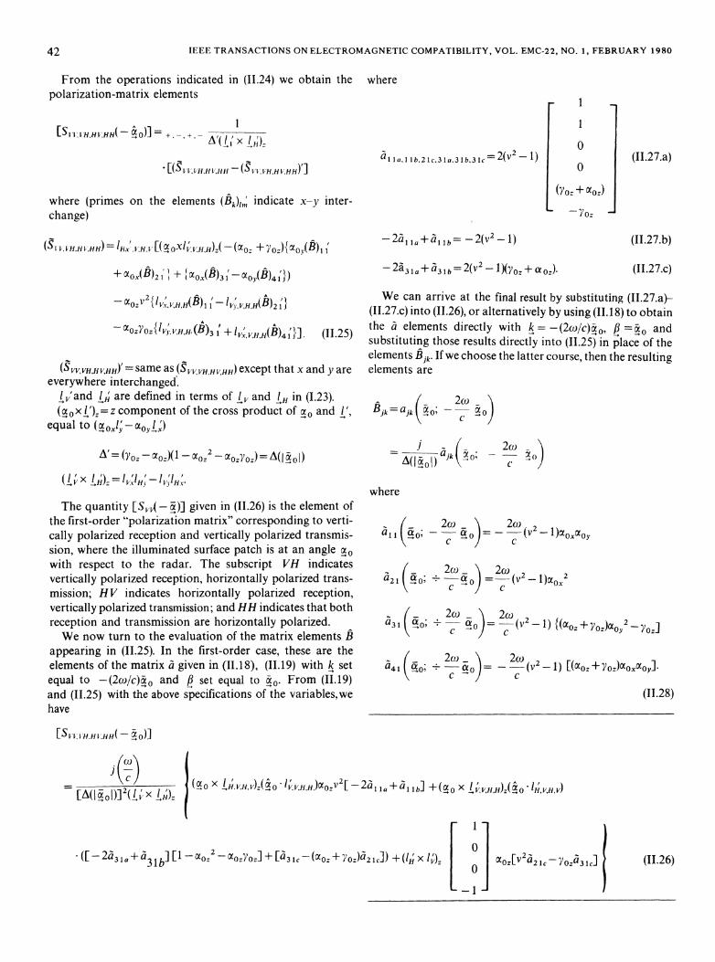
From the operations indicated in (11.24) we obtain thepolarization-matrix elements
cx~~~~x 4IS t l'.H.H I;HH( -A° [S+ I' +H H -'(S| k|)
(USVV. VH,HV.HH (SVV,VHHV.HI;HY)]
where (primes on the elements (Bk)mI, indicate x-y inter-change)
(S VLIH.H ;HH) = 'fix',1';HJ[(VOxlO..VH,H)z(-1(%z + /o_){ o (B) I1
+ xO (B)2 l + l OOX(B)3 1-XOY((B)4 I'})
lV VH,H(B)1 I- VH,H
OCOZ70Z VH,H v V,H(ThA'-ozYoz{lv),vHH (B)3 I'+ lv,vHH(B)4 }]. (1125)
(SVV,VH,HV,HH)' = same as(SVVVH,HVHH) except that x and y areeverywhere interchanged.
1v'and LH are defined in terms of lv and IH in (1.23).(a 0x L')z= z component of the cross product of ao and 1',
equal to (a oXl'-ooy I
A'(~0~-x4( -OryzAI(_CXI)Ax = 'OZH)=A(- a
('IV X I1 H')- H1'
V/ '-IV H X .
The quantity [Svj(- 5)] given in (11.26) is the element ofthe first-order "polarization matrix" corresponding to verti-cally polarized reception and vertically polarized transmis-sion, where the illuminated surface patch is at an angle x
with respect to the radar. The subscript VH indicatesvertically polarized reception, horizontally polarized trans-mission; HV indicates horizontally polarized reception,vertically polarized transmission; and HH indicates that bothreception and transmission are horizontally polarized.We now turn to the evaluation of the matrix elements B
appearing in (11.25). In the first-order case, these are theelements of the matrix ai given in (11.18), (11.19) with k setequal to -(2wo/c)ao and / set equal to ao. From (11.19)and (11.25) with the above specifications of the variables,wehave
(II.27.b)-2al la + al lb- -2(v2-1)
-2a3 la + a3 lb = 2(V2 - 1)(y0z + 0 z). (II.27.c)
We can arrive at the final result by substituting (II.27.a)-(II.27.c) into (11.26), or alternatively by using (11.18) to obtainthe a elements directly with k =-(2w,/c) 0, -a 0 andsubstituting those results directly into (11.25) in place of theelements Bjk. If we choose the latter course, then the resultingelements are
Ba(i 2wB =a LX
-(zl aJk(I °;A(I(0ik 01O -
2wo )c Jt
where
a 1 2-do a) -(v)oxaoy
a21 (a0; + 2) =2C(V2-l)%ox
2w _(t;2cotO)= 2(t)(21 (O o)O y
a3l (c 0; *_0O)=__(V2 _ J (aoz + YOZ)aoI2 y
-a.0; + -ao)= -2W(21) [(%Z+Y0Z)Vo Y].
(11.28)
jc(-01co)]2( l , x I )z |(0 H.VH,V)Z(o IVHH)V -O Ia + a 1 Ib] +(O x V,'V,H,H)z( OH VH,V)
RAEMER AND PREIS: RADAR RETURNS FROM ROUGH SEA SURFACE
Substitution of (11.28) into (11.25) yields
[SVVIJH,HVIHH( a- l")
2j(-)aO(v2 - 1)
=-(A( I ia 1)]2( l, X I ):[
1 H.1'.1I.V'X -1I V.VH.H)z[(l --kIO.-o )V2 + =2]
(11.29)
4') = spherical angles of the illuminated point on the surfacerelative to the radar in the S' system (whose z' axis is along thepeak of the antenna beam)
l. =cos 6 cos V cos D- sin 6 sin y
1 =- cos y sin qD1,'= sin 6 cos T cos 4) + cos 6 sin /
IHX=- COS 6 sin 4I
1H -sin 6 sin (D
IHy = - cos(
The quantities in (11.28) are defined below.
v complex refractive index of the mediumCl (angular) radar frequencyc free-space velocity of light
\1 2o) = ("'oz-aoz)(1 - cx2oz 7O(ZT)
[O= toxl4o
L%OzJ
[OtOX]
IVx, V)Hx,HY =I Vx,Vy,Hx,H v Vz,VH,H%Ox,O)y,Ox,OyCXOZ
,H X V')z (-I V X 1 H)z = IHX'IVJ' IHY'lVX
(L x V) = ( xH X z =x
( 0 x V,H)Z = CxOxlVy',HV %ay Vx,Hx
-aO.L Hx=%OxlVx.Hx +aoylVy,Hy-
The specialization of (11.29) to a perfectly flat sea surfaceimplies that
H =H(x", y") = mean surface as a function of (x", y"), thehorizontal coordinates in the S" system (whose z" axis isperfectly vertical and whose (x", y") plane is along thehorizontal sea surface
V"H=x-"H + A"H .
Cos 6=I
v1 +IV"H12H.cosD "H sinIV"Hl
X exaHHHH"=ay i
sin 6= V"fHH "H
lvf l+V'l
H(x", y")=O.
Choosing to set Hy- identically to zero and allowing Hx tobecome arbitrarily small (just an arbitrary choice of coor-dinate orientation which does not affect the end results), weobtain
cos'D=1 sineF=0 IV'HI=0
cos 6=1 sin 6=0
aOX=sin 0' cos 4' cos y + cos 0' sin y
Y= - sin 0' sin 4'
°- -|{1 {[sin2 0'(cos2 4' cos2 +sin2 ')+COS2 6' sin2 y + 2 sin 0' cos 0' cos 4' cos y sin y]}Yo= ±V 2
0X =sin O' cos 4' (cos 6 cos y cos (1)-sin 6 sin y)
+sin 0' sin 4' (-cos 6 sin (D)
+cos 0' (cos 6 sin y cos D + sin 6 cos y)
ao0y=sin 6' cos 4' (-cos y sin (D)
+ sin 0' sin 4' (-cos D)+cos 0' (-sin y sin (D)
0(Oz 10
y0. 2 ~2aoz =- A
y = angle of peak of antenna beam relative to the vertical (0',
lvx=Cos y IVY0 lv,= sin y 1Hx=0
1H)-= 1 1Hz 0.
Substitution of (11.30) into (11.29) yields the flat-surface formof the polarization matrix given by (la)-(lc).
REFERENCES[1] G. R. Valenzuela, "Depolarization of E-M waves by slightly rough
[21 J. W. Wright, "A new model for sea clutter," IEEE Trans. Antennas
Propagat., vol. AP- 16, pp. 2 17-223, Mar. 1968.
[3] D. E. Barrick, and W. H. Peake, "A review of scattering from surfaces
with different roughness scales", Radio Sci., vol. 3, no. 8, pp. 865-868,Aug. 1968.
(11.30)
43
27Ojoc0: + TO:X ocOX -11 'V. V.H.H.):( &-I- 0 - 1, H'. 1'. II I ) ))
IEEE TRANSACTIONS ON ELECTROMAGNETIC COMPATIBILITY, VOL. EMC-22, NO. 1, FEBRUARY 1980
141 (G. R. Valenzuela, "Scattering of electromagnetic waves from a tiltedslightly rough surface," RadioSci., vol. 3, no. I I, pp. 1057-1066, Nov.1968.
f51 G. R. Valenzuela and M. B. Laing, "Study of Doppler spectra of radarsea echo, " J. Geophys. Res., vol. 75, no. 3, pp. 551-563, Jan. 20, 1970.
161 G. R. Valenzuela, "The second order Doppler spectrum of radar sea echofor frequencies above VHF, inAGARD Conf. Proc. No. 144 (EM WaveProp. Involving Irregular Surfaes and Inhomogeneous Media), TheHague, Netherlands, pp. 25-29, Mar. 1974.
171 ,"Effect of capillarity and resonant interactions on the second orderDoppler spectrum of sea echo," J. Geophys. Res., vol. 79, no. 33, pp.
5031-5037, Nov. 20, 1974.[81 S. 0. Rice, "Reflection of electromagnetic waves from slightly rough
surfaces," Commun. Pure. Appl. Math., vol. 4, 2/3, pp. 351-378, 195 1.191 H. R. Raemer, "A comprehensive analytical study of radar returns in the
presence of a rough sea surfce," 1977; to be published as NRL scientificreport.
[101 J. K. Parks, "Towards a simple mathematical model for microwaveback-scatter from the sea surface at near vertical incidence". IEEETrans. Antennas Propagat., vol. AP- 12, pp. 590-605, Sept. 1964.
1111 1. M. Fuks, "Towards a theory of radio wave scattering at a rough seasurface," Izvestiya VUZ Radiofizi ka (USSR), vol. 9, no. 5, pp. 876-887, 1964.
[121 J. W. Wright, "Backscattering from capillary waves with application to
[ 131 F. G. Bass, 1. M. Fuks, A. 1. Kalmykov, 1. E. Ostrovsky, and A. D.Rosenberg, "Very high frequency radiowave scattering by a disturbedsea surface", IEEE Trans. Antennas Propagat., vol. AP- 16, Sept. 1968.(a) Part 1: "Scattering from a slightly disturbed boundary," pp. 554-559.(b) Part II: "Scattering from an actual sea surface," pp. 560-568.
[141 N. W. Guinard and J. C. Daley, "An experimental study of sea cluttermodels," Proc. IEEE, vol. 58, pp. 543-550, Apr. 1970.
1151 G. R. Valenzuela, M. B. Laing, and J. C. Daley, "Ocean spectra for thehigh-frequency waves as determined from airborne radarmeasurements," J. Marine Res., 29, no. 2, pp. 69-83, 197 1.
1161 N. W. Guinard, J. T. Ransone, and J. C. Daley, "Variation of the NRCSof the sea with increasing roughness," J. Geophys. Res., vol. 76, no. 6,pp. 1525 1538, Feb. 20, 197 1.
[171 A. A. Zagorodnikov, "Dependence of the spectrum of a radar signalscattered by sea surface on the size of the illuminated area and the strengthof waves, " Radio Eng. Electron Phys., vol. 17, no. 3, pp. 369-377, Jan.1972.
[181 M. W. Long, "On a two-scatterer theory of sea echo," IEEE G-AP,AP-22, No. 5, pp. 662-666, Sept. 1974.
[191 A. A. Zagorodnikov, "On the components of spatial spectrum of a radarsignal scattered by the sea," Radio Eng. Electron Phys., vol. 19, no. 2,pp. 119-121,Feb. 1974.