Assessing and Predicting the Impact of Energy Conservation ...742538/FULLTEXT01.pdf · 3 Impact...

Master of Science Thesis

KTH School of Industrial Engineering and Management

Energy Technology EGI-2014-086MSC EKV1053

Division of Heat and Power Technology

SE-100 44 STOCKHOLM

Assessing and Predicting the Impact

of Energy Conservation Measures

Using Smart Meter Data

Sophie Collard

2

Master of Science Thesis EGI 2014: 086MSC

EKV1053

Assessing and Predicting the Impact of Energy

Conservation Measures Using Smart Meter Data

Sophie Collard

Approved

29th August 2014

Examiner

Dr. Peter Hagström

Supervisor

Dr. Peter Hagström

Commissioner

Contact person

Abstract

Buildings account for around 40 percent of the primary energy consumption in Europe and in the United

States. They also hold tremendous energy savings potential: 15 to 29 percent by 2020 for the European

building stock according to a 2009 study from the European Commission. Verifying and predicting the

impact of energy conservation measures in buildings is typically done through energy audits. These audits

are costly, time-consuming, and may have high error margins if only limited amounts of data can be

collected. The ongoing large-scale roll-out of smart meters and wireless sensor networks in buildings gives

us access to unprecedented amounts of data to track energy consumption, environmental factors and

building operation. This Thesis explores the possibility of using this data to verify and predict the impact of

energy conservation measures, replacing energy audits with analytical software. We look at statistical analysis

techniques and optimization algorithms suitable for building two regression models: one that maps

environmental (e.g.: outdoor temperature) and operational factors (e.g.: opening hours) to energy

consumption in a building, the other that maps building characteristics (e.g.: type of heating system) to

regression coefficients obtained from the first model (which are used as energy-efficiency indicators) in a

building portfolio. Following guidelines provided in the IPMVP, we then introduce methods for verifying

and predicting the savings resulting from the implementation of a conservation measure in a building.

3

Table of Contents

1 Introduction ........................................................................................................................................................... 5

1.1 Context ......................................................................................................................................................... 5

1.2 Machine learning ......................................................................................................................................... 6

1.3 Project background ..................................................................................................................................... 7

1.4 Objectives ..................................................................................................................................................... 8

1.5 Report structure .......................................................................................................................................... 8

2 Regression models ................................................................................................................................................ 9

2.1 Models 1 and 2 ............................................................................................................................................ 9

2.2 Linear regression against heating degree days ......................................................................................10

2.2.1 The simple linear model ......................................................................................................................10

2.2.2 Model fitting using the normal equations .........................................................................................12

2.2.3 Assessing model accuracy ...................................................................................................................13

2.2.4 Assessing parameter estimates and predictions accuracy ...............................................................14

2.2.5 Confidence and prediction intervals ..................................................................................................14

2.3 Linear regression with additional predictors .........................................................................................15

2.3.1 Qualitative predictors ...........................................................................................................................16

2.3.2 Transformations ...................................................................................................................................16

2.3.3 Model fitting using batch gradient descent ......................................................................................17

2.3.4 Model fitting using stochastic gradient descent ...............................................................................20

2.3.5 Feature scaling .......................................................................................................................................21

2.3.6 Assessing model accuracy ...................................................................................................................22

2.3.7 Assessing parameter estimates and predictions accuracy ...............................................................24

2.3.8 Confidence and prediction intervals ..................................................................................................24

2.4 Regularization and predictor selection...................................................................................................24

2.4.1 LASSO regularization ..........................................................................................................................25

2.4.2 Model fitting using coordinate-wise gradient descent ....................................................................26

2.5 Outliers and high-leverage points detection .........................................................................................27

2.5.1 Outliers ...................................................................................................................................................27

2.5.2 High leverage points ............................................................................................................................28

3 Impact Assessment Tool and Recommendation Engine .............................................................................29

3.1 IPMVP guidelines for ECM impact assessment ..................................................................................29

3.2 ECM impact assessment ..........................................................................................................................30

3.2.1 Uncertainty of the estimates ...............................................................................................................30

3.3 ECM impact prediction ...........................................................................................................................31

3.3.1 Routine ECMs ......................................................................................................................................31

3.3.2 Non-routine ECMs ..............................................................................................................................32

4

4 Conclusion and scope for improvement .........................................................................................................34

4.1 Algorithm selection for regression models ...........................................................................................34

4.2 Current implementation and limitations of the Impact Assessment Tool and Recommendation

Engine 34

4.3 Scope for Recommendation Engine improvement .............................................................................35

References.....................................................................................................................................................................36

5

1 Introduction

This chapter presents the reader with the necessary information to understand the work documented in the

following chapters. Section 1.1 depicts the context in which the work took place. No previous exposure of

the reader to machine learning is assumed. Thus, section 1.2 constitutes a brief introduction to the topic

and provides definitions for supervised learning, unsupervised learning, regression, classification, parametric

methods and non-parametric methods. Section 1.3 presents the project background, while objectives are

detailed with in section 1.4. Finally, section 1.5 outlines the structure of the present document.

1.1 Context

In The Third Industrial Revolution, bestseller author Jeremy Rifkin posits that industrial revolutions arise from

the convergence of new communication technologies and new energy systems. In the midst of the First

Industrial Revolution at the dawn of the 19th century, the advent of steam-powered machinery

revolutionized manufacturing and transportation. The printing press became the preferred medium for

information diffusion while railroads enabled the circulation of people and mass-manufactured goods over

long distances in virtually no time. Coal, cleaner and denser than wood, fueled the steam engines that

propelled Europe, North America and Japan into the Industrial Age. In the early 20th century, electrification

and oil-powered internal combustion engines laid the foundations of the Second Industrial Revolution. New

electronic communication systems – first the telephone, later radio and television – were adopted and the

automobile became the preferred mode of transportation of workers commuting daily between cities and

sprawling residential suburbs. Rifkin predicts that the first half of the 21st century will see the onset of a

Third Industrial Revolution, resulting from the convergence of Internet and renewable energy technology.

He depicts an energy internet in which buildings are transformed into micro power plants harnessing locally

available renewable energy sources and share electricity with one another, much like we share bits of

information online today (Rifkin J 2011, p. 2).

The mutation of our centralized energy system into an energy internet – often referred to as smart grid – has

already started. A key building block of smart grids is smart metering: the deployment of electricity meters

that enable two-way communication between consumers and producers. Smart meters record and transmit

consumption data in real-time to producers, facilitating the implementation of demand response

mechanisms which become essential when large shares of intermittent energy sources are integrated into

the grid. In Europe and in the United States, the roll-out of smart meters is well underway. The Directive

2009/72/EC proposed by the European Commission as part of the Third Energy Package in 2009 mandates

that at least 80 percent of electricity consumers be equipped with intelligent metering systems by 2020

(Directive 2009/72/EC, L 211/91). A report by the Joint Research Center of the European Commission

reveals that in September 2012, over € 5 billion had been invested in smart metering in the 27 E.U. Member

States, Switzerland and Norway. The authors estimate that an additional € 30 billion will be spend on the

deployment of 170 to 180 million smart meters in the Member States by 2020 (Giordano V et al. 2013, p. 3

& 8). In a 2014 study commissioned by Siemens from Utility Dive to survey 527 U.S. electricity

professionals, 38 percent of the respondents worked for utilities that had deployed smart meters in a least

half their customers’ buildings. Only 8 percent worked for utilities that had not deployed any smart meter

at all (Utility Dive 2014, p.6).

Amidst the Big Data phenomenon, ideas on how to extract value from the vast amounts of data collected

by smart meters are springing up. Of particular interest is the potential for improving energy efficiency in

buildings. Buildings account for about 40 percent of the total primary energy consumption in Europe

(Directive 2010/31/EU, L 153/13) and in the US (Waide P et al. 2007, p. 8). They also hold tremendous

savings potential: 15 to 29 percent by 2020 for the European building stock according to Eichhammer W

et al. (2009, p. 9). When coupled with analytical methods, smart meter data could be turned into actionable

insights encouraging consumers to save energy. It could be possible to detect an unusually high electricity

consumption in a home, which might indicate that the occupants forgot to turn off some appliance. A

warning could then be sent to the occupant’s phone to inform him of the problem. Load disaggregation

6

algorithms could let occupants monitor the electricity consumption of individual devices and inform them

of which appliances and behaviors have the greatest influence on their consumption. Appliance-specific

real-time feedback is estimated to yield about three times greater savings than household-specific feedback

on utility bills (Armel K C et al. 2012, p. 6). If aggregated into the same data set, consumption data from a

large number of buildings could enable comparisons between different occupant behaviors, building uses,

appliance manufacturers, energy efficiency measures, etc. The possibilities are virtually endless and new

applications are likely to emerge as smart meters make their way into every building.

1.2 Machine learning

Machine learning is branch of artificial intelligence defined in 1959 by Arthur Samuel as “a field of study

that gives computers the ability to learn without being explicitly programmed.” Interest in machine learning

arose from the need for computer programs capable of executing tasks that would be prohibitively difficult

to describe in a set of instructions. An example of such task is detecting whether a particular object is present

in a picture. Different specimens belonging to a same object category – say, cars or dogs – could come in

many different shapes and colors and the program would need to recognize any combination of these. In

addition, the object could be depicted under infinitely many different angles. Although extremely complex

to formulate explicitly, such tasks are easily accomplished by the human brain thanks to its faculty to extract

patterns from the vast amounts of information it receives.

A sub-branch of machine learning known as supervised learning attempts to mimic the brain’s behavior by

using large amounts of data to train algorithms to perform a particular task rather than explicitly writing

down the instructions to execute it. The training data consists of inputs, such as an array containing

information about the color of each pixel in a digitized picture, and their associated outputs, such as whether

or not a particular object is present in the picture. Supervised learning algorithms process this data to identify

traits that relate a particular input characteristic to a particular output (Nilsson N J 1998, p. 5). Once trained,

the algorithm can be used to predict the output most likely associated with a new input. Another sub-branch

of machine learning known as unsupervised learning uses training data containing only inputs, without any

associated outputs, and attempts to identify clusters in the data (Nilsson N J 1998, p. 6). Again, this faculty

can be linked to the human brain’s behavior, which can easily assess how similar or dissimilar two objects

are without having been given any label for either of these objects.

Supervised learning algorithms can be divided into regression and classification algorithms, based on the nature

of the output they are trying to predict. While regression algorithms attempt to predict a quantitative and

continuous output, classification algorithms are used to predict a discrete output which may be quantitative

or qualitative (Gareth J et al. 2013, p. 28). However, the input needs not be of the same nature as the output,

and both regression and classification algorithms may use input that is quantitative, qualitative, or a

combination of both. A regression algorithm could for instance attempt to predict house prices based on

square footage (quantitative, continuous), number of bedrooms (quantitative, discrete) and borough

(qualitative). A classification algorithm could try to predict whether or not a student will get admitted to a

particular college based on the student’s high-school GPA (quantitative, continuous), number of Advanced

Placement courses taken (quantitative, discrete) and type of extracurricular activities the students takes part

in (qualitative).

Further distinction can be made between parametric and non-parametric algorithms. Parametric algorithms

assume that there exist a relationship between the input 𝑥 and output 𝑦 which can be expressed by some

mathematical function 𝑓 such that 𝑦 = 𝑓(𝑥) + 𝜖. Parametric algorithms thus require an assumption about

the shape of 𝑓 (linear, quadratic, etc.) and seek to estimate the parameters of 𝑓 that yield the best data fit

(Gareth J et al. 2013, p. 21). In contrast, non-parametric algorithms make no assumption about the shape

of 𝑓 (Gareth J et al. 2013, p. 23). There exist some algorithms that combine parametric and non-parametric

methods and are referred to as semi-parametric. An example of such algorithm is spline regression. Splines are

piecewise polynomials connected to one another at certain points. While spline regression makes no

assumptions about the overall shape of the curve is attempts to fit, the piecewise polynomials making up

7

the spline do have parameters. A benefit of parametric methods is that they produce estimates of parameters

which can be used to interpret the relationship between the input and output. In the case of simple linear

regression (see section 2.2), the parameter known as the intercept can be interpreted as the value of 𝑦 when

𝑥 = 0 while the parameter known as the slope can be interpreted as the change in 𝑦 resulting from a one-

unit change in 𝑥.

1.3 Project background

This Thesis was conducted in collaboration with EnergyDeck, a London-based startup that develops

software as a service to help building managers and occupants track and analyze their energy and resources

consumption. Its customer base consists of home owners, tenants associations, SMEs, corporate and public

organizations, utilities, retailers, brokers and consultants. A number of EnergyDeck users have expressed

an interest in analytical tools that would let them predict and verify the impact of energy conservation

measures1 (ECMs) on their consumption. In response, the company is currently working on the

development of an ECM Impact Forecasting and Validation Tool which will include, among other

functionalities, an Impact Assessment Tool and a Recommendation Engine. The Impact Assessment Tool

will let users compare the energy consumption in their building before and after the implementation of a

conservation measure. It will provide them with an estimate of the net savings attributable to the ECM since

its implementation and let them visualize the change in consumption over time. The Recommendation

Engine will forecast the net savings that different ECMs would result in if implemented in a specific building

and recommend to the user the most appropriate measures to consider if he wishes to reduce his

consumption.

In addition to consumption data, the company collects environmental data and information regarding

building operation and characteristics from its users. This data will be used to model the dependency of

energy consumption on environmental and building operation variables, which will allow separating the

impact of an ECM on a building’s energy consumption from that of other factors. The resulting set of

model parameters will then be used by the Impact Assessment Tool to estimate the net savings attributable

to a conservation measure. The parameters will also serve as indicators of a building’s energy efficiency and

be used in a second model to measure the impact of building characteristics on efficiency. The results from

the second model will be used by the Recommendation Engine to forecast the impact of a particular measure

– typically a change in building operation or characteristics – on energy consumption. Figure 1 shows how

the different modules are connected together. A clustering module will be added before the second model

in order to group buildings by type (e.g.: single-family house, office building with 5 or more floors), country,

and other properties which may significantly affect energy consumption patterns.

1 In the context of this project, energy conservation measure refers to any retrofit measure, change in equipment operation, or change in occupants’ behavior that holds potential for energy savings.

8

Figure 1: ECM Impact Forecasting and Validation Tool

1.4 Objectives

The goal of this Thesis is to develop a prototype of the ECM Impact Forecasting and Validation Tool. This

report documents the selection of appropriate algorithms for the development of the following modules

shown in Figure 1: Model 1, Model 2, Impact Assessment Tool and Recommendation Engine. The

clustering module was not implemented for the time being as clustering only becomes feasible with very

large portfolios of buildings. The search for suitable statistical analysis techniques and optimization

algorithms to build Model 1 and Model 2 was constrained by the following objectives:

high interpretability

ease of implementation

low running time

compatibility with high-dimensional data

A high interpretability is crucial if, in addition to being used by Model 2 and by the Impact Assessment

Tool, the parameters of Model 1 also serve as indicators of energy efficiency and are displayed to the users.

In addition to non-parametric methods such as k-nearest neighbors, parametric methods with low

interpretability such as splines, artificial neural networks and support vector regression were ruled out in

favor of ordinary least squares regression. Ease of implementation refers to the ease with which a particular

algorithm can be coded. Computationally elegant algorithms which can be implemented with a minimal

amount of code lines were favored in an effort to enhance code readability and maintainability. Running

time refers to the asymptotic time complexity of an algorithm and should naturally be kept as low as possible.

Finally, compatibility with high-dimensional data is necessary since Model 1 and Model 2 will sometimes

have to work with data sets containing a greater number of predictors than observations.

1.5 Report structure

Chapter 2 documents the evolution of Model 1 and Model 2 from a simple linear model to multivariate

models that use L1 regularization to perform predictor selection and prevent overfitting. Chapter 3 deals

with the development of the Impact Assessment Tool and of the Recommendation Engine. Finally, chapter

4 summarizes the work done and provides recommendations for the continuation of this project.

9

2 Regression models

This chapter documents the development of the two regression models, Model 1 and Model 2, shown in

Figure 1. Section 2.1 briefly presents the purpose of both models. In section 2.2, simple linear regression

against heating degree days (HDD) is introduced along with a fitting method known as ordinary least squares

which uses the normal equations to fit a linear function to the data. In section 2.3, the simple linear model

is expanded with the addition of multiple explanatory variables, including qualitative predictors and

transformations. Two variants of an alternative fitting method – gradient descent – are introduced, which

are computationally more efficient than the normal equations for models that use a very large number of

explanatory variables. A regularization technique known as the LASSO is presented in section 2.4, which

helps prevent overfitting while also improving model interpretability by filtering out some of the predictors.

Finally, section 2.5 focuses on the detection of outliers and high leverage points which can affect linear

models.

2.1 Models 1 and 2

Model 1 is used to find a function mapping environmental and operational data to the energy consumption

of a specific building. Modeling the dependency of energy consumption on these factors makes it possible

to isolate the impact of an ECM on the building’s energy consumption. Model 1 is a multivariate linear

model of the form:

𝑦 = 𝛽0 + ∑ 𝑥𝑗𝛽𝑗

𝑛

𝑗=1

+ 𝜖

2.1

where 𝛽 = (𝛽0, 𝛽1, … , 𝛽𝑛)𝑇 is a set of unknown parameters used by the Impact Assessment Tool to

estimate the net savings attributable to a conservation measure, 𝑦 is a column vector containing

consumption measurements collected over time from the building’s smart meter(s), and 𝑥𝑗 is a column

vector containing measurements of a certain input variable 𝑗 (e.g.: HDD, number of occupants, etc.)

collected at the same time as the corresponding consumption measurement. The sets of 𝛽 parameters

computed for several different buildings are then grouped together and used as energy efficiency indicators

in Model 2 to measure the impact of building characteristics on energy efficiency. Model 2 is also a

multivariate linear model of the form:

𝑏 = 𝜗0 + ∑ 𝑐𝑘𝜗𝑘

𝑙

𝑘=1

+ 𝑎 ∑ 𝑐𝑘𝜗𝑘

𝑝

𝑘=𝑙+1

+ 𝜖

2.2

where 𝜗 = (𝜗0, 𝜗1, … , 𝜗𝑝)𝑇

is a set of unknown parameters used by the Recommendation Engine to

forecast the impact of a conservation measure on a particular building’s consumption, 𝑏 is a column vector

containing the 𝛽𝑗 parameter estimate for every building in a portfolio, and 𝑐𝑘 is a column vector containing

information about characteristic 𝑘 (e.g.: outer walls U-value, type of heating system, etc.) of the

corresponding building.

As suggested by Kavousian A et al. (2013), some of the building characteristics in Model 2 are multiplied by

the corresponding building’s gross floor area 𝑎. This is necessary as there exist interactions between some

of the characteristics of a building and its gross floor area. For instance, with equal outer walls U-values, a

larger building will likely have a larger 𝛽𝐻𝐷𝐷 parameter mapping the number of HDD to its energy

10

consumption. In other words, for the same increase in the number of HDD, a larger building will see a

greater increase in its energy consumption because the space to be heated is larger and because increased

envelope surface leads to greater losses. Conversely, some building characteristics, such as the number and

rated power of refrigerators, do not interact with gross floor area. A certain refrigerator model will draw the

same amount of power, regardless of the size of the building it is placed in.

2.2 Linear regression against heating degree days

Space heating accounts for a significant share of the primary energy consumption in buildings: around 29

percent in residential buildings and 11 percent in commercial buildings in the US (Waide P et al. 2007, p. 9).

Space heating requirements in a building can be expressed in terms of HDD, which are dependent on

outdoor temperature. A simple algorithm for computing HDD is:

𝐻𝐷𝐷 = {

𝑇𝑏𝑎𝑠𝑒 − 𝑇𝑎𝑣𝑔 if 𝑇𝑎𝑣𝑔 ≤ 𝑇𝑏𝑎𝑠𝑒

0 if 𝑇𝑎𝑣𝑔 > 𝑇𝑏𝑎𝑠𝑒

2.3

where 𝑇𝑏𝑎𝑠𝑒 is the outdoor temperature below which space heating is required and 𝑇𝑎𝑣𝑔 is the daily average

outdoor temperature. Although other algorithms exist for computing HDD, all tend to yield values which

are roughly linearly dependent on daily average outdoor temperature below a base temperature.

Knowing the correlation between outdoor temperature and space heating demand – that is, how much more

energy is consumed with each additional HDD – the temperature-dependent part of a building’s energy

consumption (assuming no space cooling requirements) can be forecasted based on outdoor temperature

readings. This correlation can be determined by fitting a linear model to consumption data and is useful to

offset weather dependent factors and track the impact of ECMs (Liu F et al. 2011).

2.2.1 The simple linear model

Let 𝑖 be a time interval greater than or equal to one day. 𝐻𝐷𝐷𝑖 denotes the cumulative heating degree days

over 𝑖. The total energy consumption 𝑦𝑖 of a building during this time interval can be modeled as:

𝑦𝑖 = 𝛽0 + 𝛽1𝐻𝐷𝐷𝑖 + 𝜖𝑖

2.4

where 𝛽0 and 𝛽1 are the base load coefficient (or intercept) and HDD coefficient (or slope), respectively. 𝜖𝑖

denotes the random error term. 𝐻𝐷𝐷𝑖 is sometimes called the explanatory variable or predictor and 𝑦𝑖 the

response variable. 𝛽0 and 𝛽1 are usually referred to as the regression coefficients or model parameters (Gareth J et al.

2013, p. 61).

When dealing with multiple readings of 𝑦𝑖 and 𝐻𝐷𝐷𝑖, such as when training a supervised learning algorithm,

Equation 2.4 can be re-written in the following matrix-vector form:

𝑦 = 𝑿𝛽 + 𝜖

2.5

where 𝑦 is a column vector of length 𝑚, 𝛽 a column vector of length 𝑛 + 1, and 𝑿 a matrix of size 𝑚 by

𝑛 + 1:

11

𝑦𝑇 = (𝑦1, … , 𝑦𝑚)

𝛽𝑇 = (𝛽0, 𝛽1)

2.6

2.7

𝑿 = [

1 𝐻𝐷𝐷1

⋮ ⋮1 𝐻𝐷𝐷𝑚

]

2.8

with 𝑚 denoting the total number of observations and 𝑛 the number of explanatory variables. The 𝑿 and

𝑦 used to estimate the regression coefficients are referred to as the training set, and a single matrix row (𝑥𝑖,

𝑦𝑖) as a training example (Ng A 2003, Ch. 1, p. 2).

The model in Equation 2.5 makes the following assumptions:

The training set is a representative sample of the whole population;

𝑦 is a linear function of 𝐻𝐷𝐷;

𝑦 is homoscedastic, i.e., all 𝑦𝑖 have the same finite variance;

all 𝜖𝑖 are approximately normal and independent, i.e., 𝐸(𝜖𝑖) = 0, 𝑉𝑎𝑟(𝜖𝑖) = 𝜎2 for all 𝑖, and

𝐶𝑜𝑣(𝜖𝑖, 𝜖𝑗) = 0 for all 𝑖 ≠ 𝑗.

In practice however, the random error єi is not known, nor are the true regression coefficients 𝛽0 and 𝛽1.

Instead, these can be estimated by fitting a linear model to multiple readings of 𝑦𝑖 and 𝐻𝐷𝐷𝑖. The estimated

energy consumption �̂�𝑖 for a new reading of 𝐻𝐷𝐷𝑖 can then be computed using the estimated parameters

�̂�0 and �̂�1:

�̂�𝑖 = �̂�0 + �̂�1𝐻𝐷𝐷𝑖

2.9

The difference between observed and estimated energy consumption values for a same reading of 𝐻𝐷𝐷𝑖 is

called a residual and denoted 𝜖�̂�:

𝜖�̂� = 𝑦𝑖 − �̂�𝑖

2.10

The residuals can be used to check whether the normal distribution and independence assumptions about

the random error 𝜖 hold true.

One way of estimating the model parameters 𝛽 that minimize the error term 𝜖 in Equation 2.5 is ordinary

least squares (OLS). OLS seek to determine �̂� so as to minimizes the residual sum of squares (RSS), which is

the sum of the squared vertical distance between each predicted value �̂�𝑖 and observed value 𝑦𝑖 .

Mathematically, the RSS is defined as:

𝑅𝑆𝑆 = ∑(𝑦𝑖 − �̂�𝑖)2

𝑚

𝑖=1

2.11

12

The vector �̂� that minimizes the RSS may be obtained analytically using the normal equations. This approach

is detailed in the next subsection.

2.2.2 Model fitting using the normal equations

The set of regression coefficients that minimize the RSS can be obtained from the normal equations:

�̂�1 =

∑ (𝑥𝑖1 − �̅�1)(𝑦𝑖 − �̅�)𝑚𝑖=1

∑ (𝑥𝑖1 − �̅�1)2𝑚𝑖=1

2.12

�̂�0 = �̅� − �̂�1�̅�1

2.13

where �̅�𝑗 and �̅� are the average values of all 𝑥𝑖𝑗 and all 𝑦𝑖 , respectively (Gareth J et al. 2013, p. 66). Equations

2.12 and 2.13 can be combined into a single expression using matrix-vector notation:

�̂� = (𝑿𝑇𝑿)−1𝑿𝑇𝑦

2.14

The normal equations minimize the RSS by taking its derivative with respect to �̂� and setting it equal to

zero (Ng A 2003, Ch. 1, p. 11). In addition to being more elegant, the matrix vector-form given in Equation

2.14 has the benefit of working with any number of explanatory variables 𝑛, so long as 𝑛 ≤ 𝑚 − 1, and can

therefore be used to compute the parameter estimates of multivariate linear regression models.

2.2.2.1 Interpretability

A major benefit of using simple linear regression is the ease with which the results can be interpreted. In

the case of linear regression against HDD, the intercept �̂�0 corresponds to the expected energy consumption

when the outdoor temperature is above or equal to the base temperature. Mathematically, one can write

�̂�0 = 𝐸(𝑦|𝐻𝐷𝐷 = 0). The slope �̂�1 corresponds to the expected change in daily energy consumption

following a 1˚C decrease in outdoor temperature below the base temperature. Mathematically, one can write

�̂�1 = 𝐸(∆𝑦|∆𝐻𝐷𝐷 = 1).

2.2.2.2 Implementation

In MATLAB, the normal equations can be implemented as follows:

beta = pinv(X'*X)*X'*y;

where pinv() is a function that computes the pseudo-inverse of a matrix.

2.2.2.3 Running time

Solving Equation 2.14 requires performing two matrix multiplications, one matrix inversion, and one

matrix-vector multiplication. Assuming that 𝑚 = 𝑛 + 1, the asymptotic time complexity of matrix

multiplication and matrix inversion using naïve algorithms is 𝑂(𝑛3), but can be reduced to 𝑂(𝑛2.8) by using

the Strassen algorithm instead. The asymptotic time complexity of matrix-vector multiplication is 𝑂(𝑛2).

As constants and lower order terms are ignored in the expression of asymptotic time complexity, Equation

2.14 has an asymptotic time complexity of 𝑂(𝑛2.8). In practice, this means that the normal equations

constitute an attractive approach for computing �̂� when the number of explanatory variables 𝑛 is small,

13

such as in the case of linear regression against HDD. However, when a very large number of predictors is

added to the model, alternative methods may prove to have shorter running times.

2.2.2.4 Compatibility with high-dimensional data

Solving the normal equations is equivalent to solving a linear system of equations in which the number of

independent equations corresponds to the number of training examples 𝑚 and the number of unknown

terms corresponds to the total number of predictors including the intercept, 𝑛 + 1. When 𝑛 + 1 > 𝑚, the

system of linear equations is underdetermined and the normal equations have more than one unique

solution. When 𝑛 + 1 is equal or almost equal to 𝑚, there is a significant risk of overfitting, that is, modeling

random errors instead of the true function mapping 𝑿 to 𝑦 (Gareth J et al. 2013, p. 239). Such situations

require using the normal equations in combination with some feature selection technique, such as stepwise

selection.

2.2.3 Assessing model accuracy

In order to assess the accuracy of the fitted model, a measure of how well predicted data matches observed

data is needed. One such measure is the coefficient of determination R², which is the fraction of variance

in the observed data explained by the model. R² takes values comprised between 0 and 1, where 1 indicates

that 100 percent of the variance is explained by the model (Gareth J et al. 2013, p. 69). Mathematically, R²

is defined as:

𝑅2 = 1 −

𝑅𝑆𝑆

𝑇𝑆𝑆

2.15

where RSS is the residual sum of squares defined in Equation 2.11 and TSS is the total sum of squares defined

as:

𝑇𝑆𝑆 = ∑(𝑦𝑖 − �̅�)2

𝑚

𝑖=1

2.16

Another frequently used measure of model accuracy is the mean squared error (MSE) defined as:

𝑀𝑆𝐸 =

1

𝑚∑(𝑦𝑖 − �̂�𝑖)2

𝑚

𝑖=1

2.17

The MSE will be small if the predicted values closely match the observed values, and will be large if some

of the predicted and observed values differ substantially (Gareth J et al. 2013, p. 30).

When R² and the MSE are computed using the same data set that was used to train the model, they are

referred to as the training R² and training MSE. However, one is typically interested in knowing how accurate

a model is at predicting the value of previously unseen (𝐻𝐷𝐷𝑖, 𝑦𝑖) examples rather than the ones already

used to train the model. This is done by computing the test R² and test MSE, and requires using a resampling

method such as cross validation (see subsection 2.3.6). Using the test R² or test MSE instead of the training

R² or training MSE to assess model accuracy is crucial when fitting complex models for which the risk of

14

overfitting is significant. However, for simple linear models such as the one introduced in Equation 2.4, the

training R² and training MSE can be considered acceptable indicators of model accuracy.

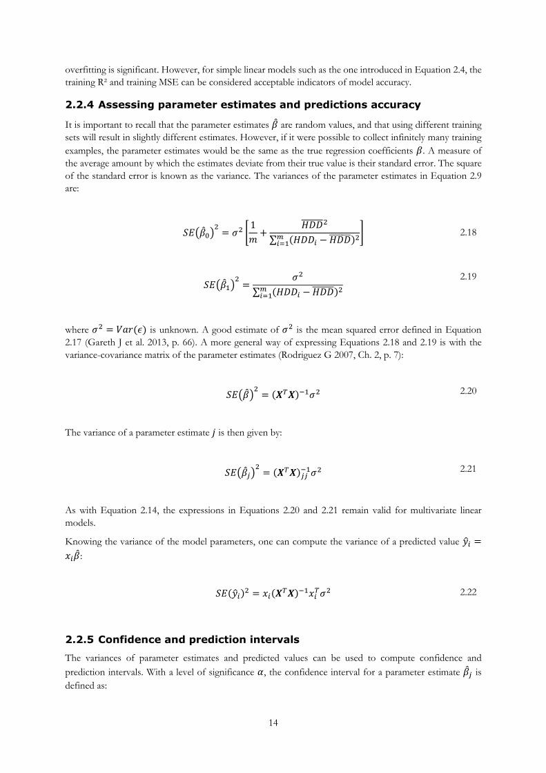
2.2.4 Assessing parameter estimates and predictions accuracy

It is important to recall that the parameter estimates �̂� are random values, and that using different training

sets will result in slightly different estimates. However, if it were possible to collect infinitely many training

examples, the parameter estimates would be the same as the true regression coefficients 𝛽. A measure of

the average amount by which the estimates deviate from their true value is their standard error. The square

of the standard error is known as the variance. The variances of the parameter estimates in Equation 2.9

are:

𝑆𝐸(�̂�0)

2= 𝜎2 [

1

𝑚+

𝐻𝐷𝐷̅̅ ̅̅ ̅̅ ̅2

∑ (𝐻𝐷𝐷𝑖 − 𝐻𝐷𝐷̅̅ ̅̅ ̅̅ ̅)2𝑚𝑖=1

]

2.18

𝑆𝐸(�̂�1)

2=

𝜎2

∑ (𝐻𝐷𝐷𝑖 − 𝐻𝐷𝐷̅̅ ̅̅ ̅̅ ̅)2𝑚𝑖=1

2.19

where 𝜎2 = 𝑉𝑎𝑟(𝜖) is unknown. A good estimate of 𝜎2 is the mean squared error defined in Equation

2.17 (Gareth J et al. 2013, p. 66). A more general way of expressing Equations 2.18 and 2.19 is with the

variance-covariance matrix of the parameter estimates (Rodriguez G 2007, Ch. 2, p. 7):

𝑆𝐸(�̂�)2

= (𝑿𝑇𝑿)−1𝜎2

2.20

The variance of a parameter estimate 𝑗 is then given by:

𝑆𝐸(�̂�𝑗)2

= (𝑿𝑇𝑿)𝑗𝑗−1𝜎2

2.21

As with Equation 2.14, the expressions in Equations 2.20 and 2.21 remain valid for multivariate linear

models.

Knowing the variance of the model parameters, one can compute the variance of a predicted value �̂�𝑖 =

𝑥𝑖�̂�:

𝑆𝐸(�̂�𝑖)2 = 𝑥𝑖(𝑿𝑇𝑿)−1𝑥𝑖𝑇𝜎2

2.22

2.2.5 Confidence and prediction intervals

The variances of parameter estimates and predicted values can be used to compute confidence and

prediction intervals. With a level of significance 𝛼, the confidence interval for a parameter estimate �̂�𝑗 is

defined as:

15

�̂�𝑗 ± 𝑡𝑚−𝑝(𝛼/2)

𝑆𝐸(�̂�𝑗)

2.23

where 𝑡𝑚−𝑝(𝛼/2)

is the two-sided Student’s t-distribution value corresponding to a level of significance 𝛼 and

𝑚 − 𝑝 degrees of freedom, with 𝑝 = 𝑛 + 1. 𝑡𝑚−𝑝(𝛼/2)

can be obtained from t-distribution tables or built-in

functions in most statistical software and is approximately equal to 2 for 𝛼 = 0.05.

For predicted values, two different intervals can be computed:

a prediction interval for a single prediction �̂�𝑖 of the value 𝑦𝑖 = 𝑥𝑖𝛽 + 𝜖𝑖 given a set of explanatory

variables 𝑥𝑖

a confidence interval for the mean predicted value �̂�𝑖 of 𝑦𝑖 = 𝑥𝑖𝛽 obtained by averaging infinitely many

single predicted values given a set of explanatory variables 𝑥𝑖

In the second case, 𝜖𝑖 disappears since the average value of the error term is zero. Prediction intervals are

used when trying to answer questions such as “given a cumulative HDD reading 𝐻𝐷𝐷𝑖 on a particular week,

what is the predicted gas consumption �̂�𝑖 of household H during this particular week?” In contrast,

confidence intervals are used to answer questions such as “what would on average be the weekly gas

consumption �̂�𝑖 of household H given a cumulative HDD reading 𝐻𝐷𝐷𝑖?” (Gareth J et al. 2013, p. 82).

The prediction interval for �̂�𝑖 is defined as:

�̂�𝑖 ± 𝑡𝑚−𝑝(𝛼/2)

√1 + 𝑆𝐸(�̂�𝑖)2

2.24

and the confidence interval as:

�̂�𝑖 ± 𝑡𝑚−𝑝(𝛼/2)

𝑆𝐸(�̂�𝑖)

2.25

2.3 Linear regression with additional predictors

Space heating is just one of many drivers of energy consumption in buildings. Other important drivers

include space cooling, water heating, lighting, ventilation, and the use of appliances. These depend on a

multitude of explanatory variables, such as cooling degree days (CDD), relative humidity, daylight hours,

occupancy, opening hours, industrial output, etc. Hence, the simple linear model introduced in section 2.2

is expanded with additional explanatory variables, such that Equation 2.4 becomes:

𝑦𝑖 = 𝛽0 + 𝛽1𝑥𝑖1 + ⋯ + 𝛽𝑛𝑥𝑖𝑛 + 𝜖𝑖 = 𝛽0 + ∑ 𝑥𝑖𝑗𝛽𝑗

𝑛

𝑗=1

+ 𝜖𝑖

2.26

Expressions of this form are used for both Model 1 and Model 2 (see section 2.1). In addition to working

with multiple quantitative predictors, the expanded model should be able to accommodate qualitative

predictors, as well as non-linear relationships between predictors and output. Methods for accommodating

these are presented in the next two subsections.

16

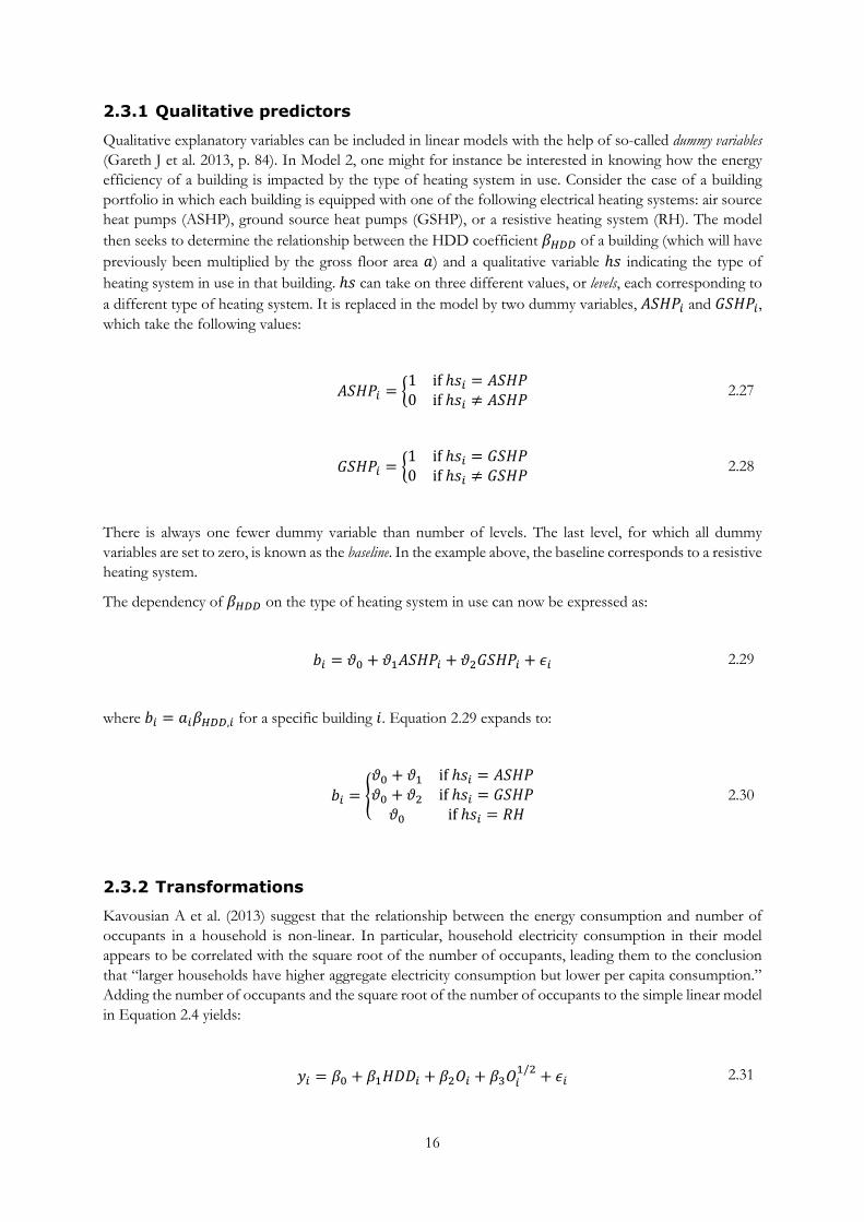
2.3.1 Qualitative predictors

Qualitative explanatory variables can be included in linear models with the help of so-called dummy variables

(Gareth J et al. 2013, p. 84). In Model 2, one might for instance be interested in knowing how the energy

efficiency of a building is impacted by the type of heating system in use. Consider the case of a building

portfolio in which each building is equipped with one of the following electrical heating systems: air source

heat pumps (ASHP), ground source heat pumps (GSHP), or a resistive heating system (RH). The model

then seeks to determine the relationship between the HDD coefficient 𝛽𝐻𝐷𝐷 of a building (which will have

previously been multiplied by the gross floor area 𝑎) and a qualitative variable ℎ𝑠 indicating the type of

heating system in use in that building. ℎ𝑠 can take on three different values, or levels, each corresponding to

a different type of heating system. It is replaced in the model by two dummy variables, 𝐴𝑆𝐻𝑃𝑖 and 𝐺𝑆𝐻𝑃𝑖,

which take the following values:

𝐴𝑆𝐻𝑃𝑖 = {

1 if ℎ𝑠𝑖 = 𝐴𝑆𝐻𝑃0 if ℎ𝑠𝑖 ≠ 𝐴𝑆𝐻𝑃

2.27

𝐺𝑆𝐻𝑃𝑖 = {

1 if ℎ𝑠𝑖 = 𝐺𝑆𝐻𝑃0 if ℎ𝑠𝑖 ≠ 𝐺𝑆𝐻𝑃

2.28

There is always one fewer dummy variable than number of levels. The last level, for which all dummy

variables are set to zero, is known as the baseline. In the example above, the baseline corresponds to a resistive

heating system.

The dependency of 𝛽𝐻𝐷𝐷 on the type of heating system in use can now be expressed as:

𝑏𝑖 = 𝜗0 + 𝜗1𝐴𝑆𝐻𝑃𝑖 + 𝜗2𝐺𝑆𝐻𝑃𝑖 + 𝜖𝑖

2.29

where 𝑏𝑖 = 𝑎𝑖𝛽𝐻𝐷𝐷,𝑖 for a specific building 𝑖. Equation 2.29 expands to:

𝑏𝑖 = {

𝜗0 + 𝜗1 if ℎ𝑠𝑖 = 𝐴𝑆𝐻𝑃𝜗0 + 𝜗2 if ℎ𝑠𝑖 = 𝐺𝑆𝐻𝑃

𝜗0 if ℎ𝑠𝑖 = 𝑅𝐻

2.30

2.3.2 Transformations

Kavousian A et al. (2013) suggest that the relationship between the energy consumption and number of

occupants in a household is non-linear. In particular, household electricity consumption in their model

appears to be correlated with the square root of the number of occupants, leading them to the conclusion

that “larger households have higher aggregate electricity consumption but lower per capita consumption.”

Adding the number of occupants and the square root of the number of occupants to the simple linear model

in Equation 2.4 yields:

𝑦𝑖 = 𝛽0 + 𝛽1𝐻𝐷𝐷𝑖 + 𝛽2𝑂𝑖 + 𝛽3𝑂𝑖1/2

+ 𝜖𝑖 2.31

17

where 𝑂𝑖 is the number of occupants in household 𝑖. It is easy to see from Equation 2.31 that the square

root of the number of occupants 𝑂𝑖1/2

is treated by the model as a third predictor with linear dependency

on the output. Thus, the expression in Equation 2.31 is still a linear model (Gareth J et al. 2013, p. 91).

When the nature of the true relationship between a new predictor and the output is unknown, one may wish

to include a few transformations of the new predictor to the set of explanatory variables in order to account

for the possibility of a non-linear relationship with the output. For every predictor 𝑥 added to Model 1 or

Model 2, the following transformations of 𝑥 are also included in the model: 𝑥2, 𝑥3, 𝑥4 and 𝑥1/2. Adding

these transformations to the model can easily lead to overfitting. Subset selection and regularization

techniques are well-known methods of filtering out irrelevant predictors and transformations in order to

prevent overfitting. A regularization technique known as the LASSO is introduced in section 2.4.

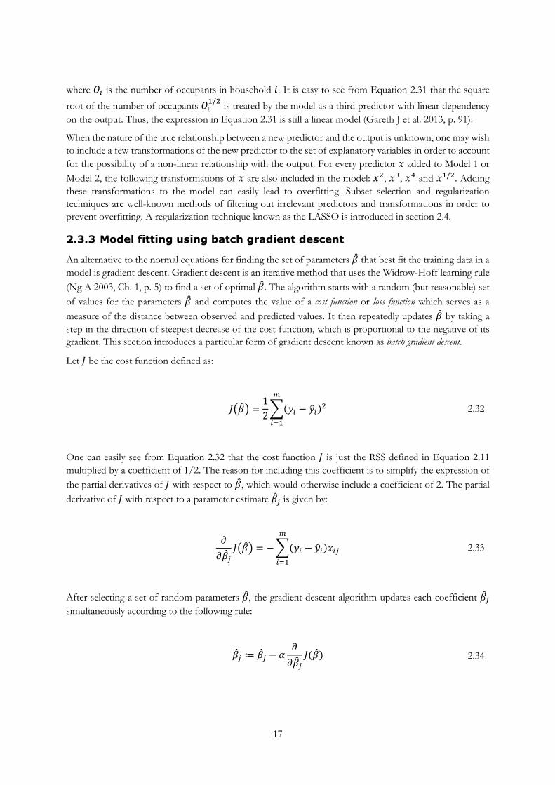
2.3.3 Model fitting using batch gradient descent

An alternative to the normal equations for finding the set of parameters �̂� that best fit the training data in a

model is gradient descent. Gradient descent is an iterative method that uses the Widrow-Hoff learning rule

(Ng A 2003, Ch. 1, p. 5) to find a set of optimal �̂�. The algorithm starts with a random (but reasonable) set

of values for the parameters �̂� and computes the value of a cost function or loss function which serves as a

measure of the distance between observed and predicted values. It then repeatedly updates �̂� by taking a

step in the direction of steepest decrease of the cost function, which is proportional to the negative of its

gradient. This section introduces a particular form of gradient descent known as batch gradient descent.

Let 𝐽 be the cost function defined as:

𝐽(�̂�) =

1

2∑(𝑦𝑖 − �̂�𝑖)2

𝑚

𝑖=1

2.32

One can easily see from Equation 2.32 that the cost function 𝐽 is just the RSS defined in Equation 2.11

multiplied by a coefficient of 1/2. The reason for including this coefficient is to simplify the expression of

the partial derivatives of 𝐽 with respect to �̂�, which would otherwise include a coefficient of 2. The partial

derivative of 𝐽 with respect to a parameter estimate �̂�𝑗 is given by:

𝜕

𝜕�̂�𝑗

𝐽(�̂�) = − ∑(𝑦𝑖 − �̂�𝑖)𝑥𝑖𝑗

𝑚

𝑖=1

2.33

After selecting a set of random parameters �̂�, the gradient descent algorithm updates each coefficient �̂�𝑗

simultaneously according to the following rule:

�̂�𝑗 ≔ �̂�𝑗 − 𝛼

𝜕

𝜕�̂�𝑗

𝐽(�̂�)

2.34

18

where 𝛼 is some predefined constant known as the learning rate. As the partial derivatives of 𝐽 with respect

to �̂� are proportional to the residuals, the second term on the right hand side of Equation 2.34 subtracted

from an estimate �̂�𝑗 becomes smaller and smaller as the distance between observed and predicted values

reduces with each iteration. Combining Equations 2.33 and 2.34 yields:

�̂�𝑗 ≔ �̂�𝑗 + 𝛼 ∑(𝑦𝑖 − �̂�𝑖)𝑥𝑖𝑗

𝑚

𝑖=1

2.35

The update in Equation 2.35 is carried out repeatedly and simultaneously for all 𝑗’s until some convergence

rule is satisfied. Updating �̂�𝑗 simultaneously for all 𝑗’s means that the value of the cost function gradient

∑ (𝑦𝑖 − �̂�𝑖)𝑥𝑖𝑗𝑚𝑖=1 is only updated at the end of a full iteration, once all �̂�𝑗 have been updated.

In general, gradient descent is susceptible to getting stuck at local minima. However, for linear regression

problems the cost function 𝐽 defined in Equation 2.32 is a quadratic function (see Figure 2) and has only

one global minimum. Thus, the gradient descent method presented above always converges to the global

minimum of 𝐽, provided that the learning rate 𝛼 is not too large (Ng A 2003, Ch. 1, p. 5).

Figure 2: 𝐽 as a function of two parameters �̂�0 and �̂�1

Selecting an appropriate learning rate 𝛼 is crucial in order to optimize convergence. If 𝛼 is too small,

convergence will be very slow. If 𝛼 is too large, the algorithm risks getting stuck or even diverging. Figure

3 shows gradient descent convergence for different values of 𝛼 using 400 iterations. In the top plots, the

blue line shows the value of 𝐽(�̂�) as a function of �̂�0 while all other parameters �̂�𝑗 are held constant. The

red line shows the path taken by the gradient descent algorithm, with start and end points. The bottom plots

show the value of 𝐽(�̂�) as a function of the number of iterations. The leftmost plots show convergence for

an optimal value of 𝛼. The algorithm converges to the minimum after about 300 iterations. The second set

of plots show convergence for a too small value of 𝛼. Convergence is very slow and the algorithm still

doesn’t reach the minimum after 400 iterations. The last two sets of plots show how the algorithm fails to

converge for too large values of 𝛼. In the third set of plots, the algorithm gets stuck. For a slightly larger

value of 𝛼 in the rightmost plots, the algorithm diverges and 𝐽(�̂�) increases exponentially with each new

iteration.

19

Figure 3: gradient descent convergence for different learning rates


Just like the normal equations, gradient descent yields a set of 𝑛 + 1 parameters for a model containing 𝑛

predictors. While interpretability is still good for models using a small number of predictors, it becomes

harder to make sense of the results with a very large set of explanatory variables. In particular, correlations

(or collinearity) between two or more predictors can make the results confusing, as the impact of one

predictor on the output may be masked by that of another predictor.


Replacing the convergence rule by a number of iterations num_iter, batch gradient descent can be

implemented in MATLAB as follows:

for k = 1:num_iter

beta = beta + alpha * ((y-X*beta)'*X)';

end

where alpha is the learning rate. Note that indexing in MATLAB starts from 1 instead of 0.


Computed simultaneously for all 𝑗’s, the expression in Equation 2.35 has an asymptotic time complexity of

𝑂(𝑚𝑛). If 𝑘 is the number of iterations required for convergence, the overall time complexity of the batch

gradient descent algorithm is 𝑂(𝑘𝑚𝑛). For models that use a moderate2 number of predictors, 𝑘 is typically

greater than 𝑛 and batch gradient descent runs slower than the normal equations. However, for models that

use a very large number of predictors, 𝑘 becomes smaller than 𝑛. In this case, batch gradient descent runs

faster than the normal equations which, assuming 𝑚 = 𝑛 + 1, have a time complexity of 𝑂(𝑛2.8) at best.


Like the normal equations, batch gradient descent has more than one unique solution when the number of

predictors (including the intercept term) exceed the number of training examples, and is susceptible to

2 As a rule of thumb, we consider 𝑛 to be moderate if 𝑛 < 10000.

20

overfitting when there are only slightly fewer predictors than training examples. In such situations, batch

gradient descent must be used in combination with predictor selection and/or regularization techniques.

2.3.4 Model fitting using stochastic gradient descent

An alternative to batch gradient descent is stochastic gradient descent. Whereas batch gradient descent requires

that the algorithm scans through the entire training set before updating �̂� – a time-consuming procedure if

the number of training examples is large – stochastic gradient descent proceeds one training example at a

time. Stochastic gradient descent is an example of an online algorithm, that is, an algorithm that can start

processing data and making progress without being handed the whole training data set at once (Nilsson N

J 1998, p. 8). In practice, this means that stochastic gradient descent often converges to the minimum value

of 𝐽 much faster than batch gradient descent (Ng A 2003, Ch. 1, p. 7).

Stochastic gradient descent requires randomly shuffling the training examples beforehand, so that the

algorithm sees as diverse training examples as possible early in the process. The algorithm proceeds by

scanning through each training example 𝑖 and updating each parameter estimate �̂�𝑗 as follows:

�̂�𝑗 ≔ �̂�𝑗 + 𝛼(𝑦𝑖 − �̂�𝑖)𝑥𝑖𝑗

2.36

The update rule in Equation 2.36 is carried out repeatedly and simultaneously for all 𝑗’s until some

convergence rule is satisfied.

Figure 4 illustrates the differences between batch gradient descent and stochastic gradient descent. The top

plots show convergence using batch gradient descent, while the bottom ones show convergence on the

same data set using stochastic gradient descent. In the leftmost plots, the blue line shows the value of 𝐽(�̂�)

as a function of �̂�0 while all other parameters �̂�𝑗 are held constant. The red line shows the path taken by

the gradient descent algorithm, with start and end points. The center plots show contour plots of 𝐽(�̂�) as a

function of �̂�0 and �̂�1 while all other parameters �̂�𝑗 are held constant. Again, the red line shows the path

taken by the gradient descent algorithm, with start and end points. The rightmost plots show the value of

𝐽(�̂�) as a function of the number of iterations.

Figure 4: differences between batch gradient descent and stochastic gradient descent

21

In the example of Figure 4, it is easy to see that stochastic gradient descent converges much faster than

batch gradient descent. While batch gradient descent requires about 300 iterations to converge, stochastic

gradient descent requires only about 8. The trade-off when using stochastic gradient descent instead of

batch gradient descent is a more noisy convergence, as can be seen from the center plots. In practice

however, this is rarely a problem.


In terms of interpretability, stochastic gradient descent suffers from the same limitations as the normal

equations and batch gradient descent: a large number of parameters is difficult to interpret, particularly when

there exist strong correlations between some of the predictors.


Replacing the convergence rule by a number of iterations num_iter, stochastic gradient descent can be

implemented in MATLAB as follows:

for k = 1:num_iter

for i = 1:m

beta = beta + alpha * ((y(i)-X(i,:)*beta)*X(i,:))';

end

end


Parsing through the entire training data set once and computing the expression in Equation 2.36

simultaneously for all 𝑗’s is an operation with a time complexity of 𝑂(𝑚𝑛). If 𝑘 is the number of iterations

required for convergence, the overall time complexity of the stochastic gradient descent algorithm is

𝑂(𝑘𝑚𝑛), the same as that of the batch gradient descent algorithm introduced in subsection 2.3.3. In practice

however, parsing through only a fraction of the training set is often sufficient to make significant progress

and the number of iterations required for convergence is often much smaller with stochastic gradient

descent than batch gradient descent (Ng A 2003, Ch. 1, p. 7). This makes stochastic gradient descent an

attractive alternative to batch gradient descent, particularly when the number of training examples 𝑚 is large.


Just like the normal equations and batch gradient descent, stochastic gradient descent requires using

predictor selection and/or regularization techniques when the number of predictors is close to or exceeds

the number of training examples.

2.3.5 Feature scaling

The parameter estimates �̂� are scale-invariant, i.e., multiplying the whole set of training examples 𝑥𝑗 for a

predictor 𝑗 by a constant 𝑐 ≠ 0 results in the multiplication of �̂�𝑗 by a factor 1/𝑐. Hence, 𝑥𝑗�̂�𝑗 always

remains constant (Gareth J et al. 2013, p. 217). In order to facilitate the convergence of gradient descent

algorithms, the training set is usually normalized and scaled as follows:

𝑥𝑖𝑗 =

𝑥𝑖𝑗 − �̅�𝑗

𝜎𝑗

2.37

22

where 𝑥𝑖𝑗 is the value of predictor 𝑗 for the training example 𝑖, �̅�𝑗 is the average value of the predictor 𝑗 and

𝜎𝑗 is its standard deviation. This procedure, known as feature scaling, reduces the number of iterations required

for convergence. Figure 5 shows contour plots of the cost function 𝐽(�̂�) as a function of two parameter

estimates �̂�0 and �̂�1. The red line shows the path followed by the stochastic gradient descent algorithm,

with start and end points. Both plots were made using the same data set, but the left plot doesn’t use feature

scaling while the right one does.

Figure 5: Stochastic gradient descent without feature scaling (left) versus stochastic gradient descent with feature scaling (right)

When the training examples for different predictors have different scales, the contours of the cost function

𝐽 are shaped like long and narrow ellipsoids. This makes the path to convergence much longer, as depicted

in the left plot in Figure 5.

2.3.6 Assessing model accuracy

The training R2 and training MSE introduced in subsection 2.2.3 may be considered acceptable indicators

of model accuracy for simple linear models. However, multivariate models that use a large number of

predictors are susceptible to overfitting, a consequence of which is that the model may perform significantly

worse on previously unseen examples than on the training set (Gareth J et al. 2013, p. 204). Thus, new

indicators are needed in order to assess how good the model is at making predictions. A resampling method

known as k-fold cross-validation is used to produce new R2 and MSE estimates for Model 1 and Model 2. This

method requires splitting the original training set into 𝑘 different sets, or folds, of similar size. Each

individual training example is randomly assigned to one and only one fold, so that no two folds may contain

the same training example. Typical values of 𝑘 are 5 or 10, depending on the size of the original training

data set (Gareth J et al. 2013, p. 184). The model is fitted using a training set consisting of 𝑘 − 1 folds while

the remaining 𝑘𝑡ℎ fold is used as a test set to compute R2 and the MSE. This procedure is repeated 𝑘 times

in total, each time using a different fold as the test set, resulting in 𝑘 R2 and MSE estimates. Test R2 and test

MSE are then computed by averaging their 𝑘 respective estimates:

𝑅2̅̅̅̅ =1

𝑘∑ 𝑅𝑖

2

𝑘

𝑖=1

2.38

23

𝑀𝑆𝐸̅̅ ̅̅ ̅̅ =

1

𝑘∑ 𝑀𝑆𝐸𝑖

𝑘

𝑖=1

2.39

When the total number of training examples in the original training set is not a multiple of 𝑘, so that the

folds may have slightly different sizes, or when comparing the test R2 and test MSE from one model to

another, it is preferable to use the so-called adjusted R2 and adjusted MSE instead of the formulas in Equations

2.15 and 2.17. Mathematically, the adjusted R2 and adjusted MSE are defined as:

𝑅𝑎𝑑𝑗

2 = 1 − (1 − 𝑅2)𝑚 − 1

𝑚 − 𝑛 − 1

2.40

𝑀𝑆𝐸𝑎𝑑𝑗 =

1

𝑚 − 𝑛 − 1∑(𝑦𝑖 − �̂�𝑖)2

𝑚

𝑖=1

2.41

As their name suggests, the adjusted R2 and adjusted MSE make adjustments for the number of training

examples and predictors used to fit the model, enabling comparisons between models fitted with training

sets of different sizes.

The need for resampling methods is illustrated in Figure 6 and Figure 7. Fitting a polynomial of degree 𝑛 to

a set of observations consisting of one explanatory variable 𝑥 and one response variable 𝑦 requires using

𝑛 − 1 transformations of 𝑥, such that the total set of predictors (excluding the intercept term) becomes

𝑥, 𝑥2, … , 𝑥𝑛−1, 𝑥𝑛. Figure 6 depicts polynomials of different degrees fitted to a same set of observations.

The true relationship mapping the input 𝑥 to the output 𝑦, shown by the black curves in the plots of Figure

6, is a polynomial of degree 3.

Figure 6: polynomials of different degrees fitted to a same set of observations

24

It is evident from Figure 6 that polynomials of degree 2, 3, 4 and 5 provide the best fit. However, there is

not much evidence that polynomials of degree 4 and 5 lead to a better fit than a polynomial of degree 3. A

polynomial of degree 1, i.e., a simple linear model, significantly underfits the data while polynomials of

degree 7 and above result in overfitting. The consequences of overfitting can be seen in Figure 7, which

shows the training MSE and test MSE as a function of the total number of predictors. Note that the intercept

term is included in the total number of predictors in Figure 7, such that a simple linear model contains 2

predictors, a polynomial of degree 2 contains 3 predictors, and so on.

Figure 7: training MSE and test MSE for polynomials of different degrees fitted to a same data set

Figure 7 shows that while the training MSE seems to be systematically decreasing with the addition of new

predictors, the test MSE decreases sharply up to a number of 3 predictors but increases again for models

using a greater number of predictors as a result of overfitting. Without the use of resampling method to

compute the test MSE, overfitting could be difficult to detect. Furthermore, using the training MSE as an

indicator of quality of fit on models suffering from overfitting would lead to an underestimation of the

prediction error made by the model. Not only does the test MSE makes it easy to identify the optimal

number of predictors in the model, it also provides an indicator of the quality of fit.

2.3.7 Assessing parameter estimates and predictions accuracy

Parameter estimates accuracy and predictions accuracy can be computed using Equations 2.21 and 2.22,

respectively, replacing 𝜎2 by the test MSE introduced in Equation 2.39.

2.3.8 Confidence and prediction intervals

Confidence and prediction intervals can be computed using Equations 2.23, 2.24 and 2.25.

2.4 Regularization and predictor selection

The advent of wireless sensor networks and the availability of cheap sensors sold by the unit have led some

building owners and managers to monitor a wide range of environmental and operational variables. Once

transformations are added to account for the possibility of a non-linear relationship between some of the

sensors’ readings and energy consumption, the number of predictors for some buildings may exceed the

number of training examples available. In such situation, the fitting methods introduced so far cannot be

used to estimate the set of model parameters �̂� as more than one unique solution exists. Even when the

number of predictors is not quite as large as the number of training examples, the significant risk of

overfitting compromises the model’s ability to make predictions. In addition, using a large number of

25

predictors greatly complicates parameters interpretation. Often times, many of the predictors have in fact

no influence on the response variable, but because of the way least squares work it is very unlikely that the

parameter estimates for these predictors be exactly zero.

The problems described in the previous paragraph can be solved with the help of so-called predictor

selection and regularization techniques. While predictor selection eliminates irrelevant predictors from the

model, regularization shrinks the parameter estimates for the least relevant predictors, effectively reducing

their impact on future predictions. Popular predictor selection techniques include forward selection,

backward selection and mixed selection. A well-known and easy to implement regularization technique is

ridge regression (Gareth J et al. 2013, p. 215), which simply requires adding a so-called penalization term to

the cost function given in Equation 2.32:

𝐽(�̂�) =

1

2(∑(𝑦𝑖 − �̂�𝑖)2

𝑚

𝑖=1

+ 𝜆 ∑ �̂�𝑗2

𝑛

𝑗=1

)

2.42

𝜆 is a constant known as the regularization parameter or shrinkage coefficient. Note that the intercept �̂�0 is not

regularized. The regularized cost function in Equation 2.42 is differentiable and can be used in combination

with batch and stochastic gradient descent techniques introduced in subsections 2.3.3 and 2.3.4. Minimizing

the expression above is equivalent to minimizing the expression in Equation 2.32 subject to ‖�̂�‖2

≤ 𝜆.

Despite shrinking the values of parameter estimates for the least relevant predictors, ridge regression does

not perform predictor selection since none of the parameter estimates are shrank exactly to zero. The next

subsection presents an alternative regularization technique known as the Least Absolute Shrinkage and

Selection Operator (LASSO), which is capable of both predictor selection and parameter regularization.

2.4.1 LASSO regularization

LASSO regularization works in a similar way to ridge regression: a regularization term is added to the cost

function which, for increasing values of 𝜆, shrinks the regression parameter estimates towards zero. In the

case of LASSO regularization however, the regularization term forces some of the parameter estimates to

be exactly zero, thus also performing predictor selection (Gareth J et al. 2013, p. 219). The LASSO is said

to yield sparse models. With LASSO regularization, the cost function becomes:

𝐽(�̂�) =

1

2(∑(𝑦𝑖 − �̂�𝑖)2

𝑚

𝑖=1

+ 𝜆 ∑|�̂�𝑗|

𝑛

𝑗=1

)

2.43

As with Equation 2.42, the intercept �̂�0 is not regularized. Minimizing the expression in Equation 2.43 is

equivalent to minimizing the expression in Equation 2.32 subject to ‖�̂�‖1

≤ 𝜆. A drawback of the LASSO

is that, unlike Equation 2.42, the expression in Equation 2.43 is not differentiable at �̂�𝑗 = 0, which

complicates the implementation of gradient descent algorithms. A suitable algorithm is introduced in

subsection 2.4.2.

Selecting an appropriate value for the shrinkage coefficient 𝜆 is crucial to optimize LASSO regularization.

For 𝜆 = 0, the regularization term in Equation 2.43 disappears and the model is fit using OLS regression

introduced in sections 2.2 and 2.3. For too large values of 𝜆, all the parameter estimates are set to zero and

the model is effectively reduced to �̂� = �̂�0. Cross-validation provides a simple method for selecting an

26

appropriate 𝜆 value. First, the regression parameter estimates �̂� are computed for a range of 𝜆 value (e.g.:

𝜆 = (0.01, 0.03, 0.1, 0.3, … )). Then, the test MSE or test R2 is computed using k-fold cross-validation, and

the appropriate 𝜆 value is selected by choosing the one which yields either the lowest test MSE or higher

test R2.

2.4.2 Model fitting using coordinate-wise gradient descent

This subsection presents the implementation by Kim J et al. (2007) of the gradient LASSO algorithm

proposed by Kim Y and Kim J (2004). Let �̂� be the set of parameter estimates such that �̂� = �̂�/𝜆. The

algorithm for coordinate-wise gradient descent with LASSO is:

1. Let �̂�𝑗 = 0 for 𝑗 = 0,1, … , 𝑛.

2. Repeat until convergence:

a. Compute the gradient of the cost function 𝐽(�̂�) defined in Equation 2.32.

b. Find (𝑗̂, 휀̂) that minimizes 휀 ∂𝐽(�̂�) �̂�𝑗⁄ for 𝑗 ∈ (1, … , 𝑛) and 휀 = ±1.

c. Let 𝑒𝑗 be the (𝑛 + 1)-dimensional vector such that the 𝑗̂𝑡ℎ element (with indexing starting from

0) is equal to 휀̂ and all the others are zero.

d. Find 𝛾 ∈ [0,1] that minimizes 𝐽(𝛾�̂� + (1 − 𝛾)𝑒𝑗).

e. Update �̂� according to �̂� ≔ 𝛾�̂� + (1 − 𝛾)𝑒𝑗.

In step 2.d., 𝐽(𝛾�̂� + (1 − 𝛾)𝑒𝑗) can be minimized, for instance, using golden section search.


A major benefit of using the LASSO is that the resulting model is sparse, that is, the regression coefficients

of the least relevant predictors are set exactly to 0. Thus, the LASSO performs predictor selection. Because

the resulting set of parameter estimates �̂� is smaller than with the methods introduced in subsections 2.2.2,

2.3.3 and 2.3.4 and because the predictors corresponding to these parameter estimates are known to have

an impact on the response variables, interpretation of the results is greatly simplified.


Replacing the convergence rule by a number of iterations num_iter, coordinate-wise gradient descent can

be implemented in MATLAB as follows:

% step 1

w = zeros(size(X,2),1);

% step 2

for k = 1:num_iter

% step 2a

grad = -((y-X*w)'*X)';

% step 2b

if min(grad(2:end)) < min(-grad(2:end))

[junk,j] = min(grad(2:end))

eps = 1;

else

[junk,j] = min(-grad(2:end))

eps = -1;

27

end

% step 2c

e = zeros(size(X,2),1);

e(j) = eps;

% step 2d

gamma = gSS(w,e);

% step 2e

w = gamma*w + (1 - gamma)*e;

end

% step 3

beta = w*lambda;

where gSS(w,e) is a function that uses golden section search to return the optimal value of 𝛾.


Step 2.a. of coordinate-wise gradient descent has an asymptotic time complexity of 𝑂(𝑚𝑛). If 𝑘 is the

number of iterations required for convergence in step 2.d., then the overall time complexity of coordinate-

wise gradient descent is 𝑂(𝑘𝑚𝑛).


The LASSO performs predictor selection and parameter regularization, which allows fitting a model on

high-dimensional data. Coordinate-wise gradient descent can be applied not only to data sets where the

number of predictors 𝑛 is almost equal to the number of training examples 𝑚, but also where 𝑛 > 𝑚 − 1.

This is especially useful in situations where many different environmental and operational variables are being

monitored but their values are recorded at a low frequency, such as daily or weekly.

2.5 Outliers and high-leverage points detection

Outliers are training examples for which the observed response 𝑦𝑖 is very far from the predicted response

�̂�𝑖 produced by the model. High-leverage points are training examples with unusual predictor values 𝑥𝑖.

Outliers and high-leverage points can arise because of defective or improperly calibrated sensors and

influence the values of parameter estimates �̂� as well as those of R2, MSE, standard errors, prediction and

confidence intervals. Thus, it is important identify and remove these data points from the training set.

2.5.1 Outliers

Outliers are identified using a method suggested by Gareth J et al. (2013, p. 97). The method requires

computing the studentized residuals, which are defined as the residuals 𝜖�̂� divided by the standard error

𝑆𝐸(�̂�𝑖) or the corresponding predictions:

𝜖�̂�,𝑆𝑇𝑈 =

𝜖�̂�

𝑆𝐸(�̂�𝑖)

2.44

The studentized residual is a measure of the number of standard deviations that separate an observation 𝑦𝑖

from its expected value �̂�𝑖 . If the assumptions about the normal distribution and independence of errors

made in subsection 2.2.1 hold true, about 99 percent of the observations should be within 3 standard

28

deviations of their expected value. Observations whose studentized residuals are greater than 3 in absolute

value, i.e. observations 𝑦𝑖 which are more than 3 standard deviations away from their expected value �̂�𝑖 , are

considered outliers and removed from the training set.

2.5.2 High leverage points

High-leverage points in simple linear models are easy to detect: they are points for which the predictor 𝑥𝑖 is

well outside the normal range of values for 𝑥. In multivariate models however, high-leverage points can be

trickier to detect. It can be that all of the individual predictors 𝑥𝑖𝑗 are well within their respective normal

range of values but that their combination is unusual. High-leverage points can be detected by computing

the leverage ℎ𝑖 of each training example 𝑖:

ℎ𝑖 = [𝑿(𝑿𝑇𝑿)−1𝑿𝑇]𝒊𝒊

2.45

ℎ𝑖 values can range from 1/𝑚 to 1, while the average of all observations is equal to (𝑛 + 1)/𝑚. Data points

whose leverage exceeds (3𝑛 + 1)/𝑚 are considered outliers and removed from the training set.

29

3 Impact Assessment Tool and Recommendation Engine

This chapter documents the development of the Impact Assessment Tool and Recommendation Engine

shown in Figure 1. Section 3.1 summarizes the International Performance Measurement and Verification

Protocol (IPMVP) guidelines for assessing the impact of ECMs in buildings. Section 3.2 details how the

savings attributable to each individual ECM implemented in a building over time are estimated by splitting

energy consumption time series into periods and fitting a set of Model 1 parameters to the data in each

period. Finally, in section 3.3, a distinction is made between routine and non-routine ECMs and methods

are provided for predicting the impact of either on a building’s consumption using the parameter estimates

of Model 1 and Model 2.

3.1 IPMVP guidelines for ECM impact assessment

The IPMVP is a guidance document describing best practice for measuring, computing and reporting

savings achieved by energy or resource efficiency projects. It provides four options for verifying the savings

resulting from the implementation of an ECM: (A) retrofit isolation: key parameter measurement, (B)

retrofit isolation: all parameters measurement, (C) whole facility, and (D) calibrated simulation (Efficiency

Valuation Organization 2012, p. 22). Options A and B require measurements of key performance parameters

driving energy use of the system affected by the ECM. Option C involves determining savings by measuring

energy use at the whole facility or sub-facility level using utility bills or meters as a source of data. This

approach typically requires regression analysis to extract the impact of independent variables, such as

outdoor temperature, on energy consumption. Option D involves simulating energy consumption at the

whole facility or sub-facility level and is applicable when no historical energy data is available. This approach

requires considerable skill in simulation. The Impact Assessment Tool developed by EnergyDeck uses

option C to assess the impact of ECMs with the help of whole building or building section energy

consumption data.

The period preceding the implementation of an ECM is referred to as the baseline period while the period

following it is known as the reporting period. Savings are computed by comparing measured energy use prior

to and following the implementation of ECMs, making suitable adjustments for changes in conditions

between the baseline and reporting periods. Adjustments can be divided between routine (e.g.: weather

conditions) and non-routine (e.g.: indoor environmental quality standards). In principle, both the baseline

and reporting periods should span a full operating cycle, from maximum energy use to minimum, in order

to represent all operating modes of the facility and fully characterize the savings effectiveness in all normal

operating modes. This typically means recording energy use for one year both before and after the

implementation of an ECM (Efficiency Valuation Organization 2012, p. 17). In practice though, this may

sometimes not be possible because a user might choose to implement an ECM in his building less than one

year after the start of data collection and wish to get an estimate of the savings as soon as possible. Thus,

the Impact Assessment Tool will sometimes have to extrapolate the results obtained from Model 1. An

uncertainty estimate is therefore provided along with savings estimates to give the user a sense of how

reliable the results are.

Estimating the savings resulting from the implementation of an ECM requires computing the so-called

adjusted-baseline consumption, which is an estimate of the energy consumption that would have taken place

during the reporting period, had the ECM not been implemented. The savings – sometimes referred to as

avoided energy use – are computed by integrating over time the difference between adjusted-baseline

consumption and reporting period consumption. Comparing the savings resulting from ECMs implemented

in different buildings, or within the same building but at a different time, can be done by normalizing the

adjusted-baseline and reporting period consumption according to some reference conditions other than

those of the reporting period.

30

3.2 ECM impact assessment

The savings – or more specifically the change in a building’s energy consumption between two periods –

attributable to ECMs implemented a different points in time can be determined by analyzing time series of

energy consumption, environmental and operational data. Time series are split into periods delimited by

ECM implementation dates, such that period 𝑞 is the period starting with the implementation of measure

𝑞 and ending with the implementation of measure 𝑞 + 1 or with the last data entry. Periods are indexed

starting from 0, with period 0 ranging from the first data point available to the implementation of the first

conservation measure. Savings attributable to each conservation measure are computed from period 1

onwards. ECM implementation is assumed to be instantaneous, i.e., ECMs are assumed to start and be

completed at the same point in time, with the full savings observable immediately after that point. In reality,

implementation can span several weeks or months and the full savings only become visible after the project

completion.

A set of regression coefficients �̂� is fitted to the data in each period. The savings in period 𝑞 attributed to

measure 𝑞 are computed by taking the sum of the differences between measured consumption in period 𝑞,

denoted 𝑦𝑞, and predicted consumption in period 𝑞 under the assumption that building energy performance

had remained the same as in period 𝑞 − 1, denoted �̂�𝑞|�̂�𝑞−1 = 𝑿𝑞�̂�𝑞−1. The measured consumption

corresponds to the reporting period consumption defined in the IPMVP, while the predicted consumption

corresponds to the adjusted-baseline consumption. Mathematically, the savings in period 𝑞 attributable to

the conservation measure 𝑞 are defined as:

�̂�𝑞|𝐸𝐶𝑀=𝑞 = 𝑿𝑞�̂�𝑞−1 − 𝑦𝑞

3.1

Similarly, the savings in period 𝑞 attributed to the conservation measure 𝑞 − 1 are computed by taking the

sum of the difference between predicted consumption in period 𝑞 under the assumption that building

energy efficiency had remained the same as in period 𝑞 − 1, �̂�𝑞|�̂�𝑞−1 = 𝑿𝑞�̂�𝑞−1, and predicted

consumption in period 𝑞 under the assumption that building energy efficiency had remained the same as in

period 𝑞 − 2, �̂�𝑞|�̂�𝑞−2 = 𝑿𝑞�̂�𝑞−2:

�̂�𝑞|𝐸𝐶𝑀=𝑞−1 = 𝑿𝑞�̂�𝑞−1 − 𝑿𝑞�̂�𝑞−2

3.2

3.2.1 Uncertainty of the estimates

Let 𝛿�̂�𝑖 denote the uncertainty associated with a single prediction �̂�𝑖 . An appropriate measure of uncertainty

for �̂�𝑖 would be the prediction interval defined in Equation 2.24, such that:

𝛿�̂�𝑖 = 𝑡𝑚−𝑝

(𝛼/2)√1 + 𝑆𝐸(�̂�𝑖)2

3.3

One can see from Equations 3.1 and 3.2 that computing savings estimates is done by adding and subtracting

predictions �̂�𝑖 from one another. When adding and subtracting values whose random error component is

assumed to be normally distributed and independent, the uncertainty of the result can be obtained by taking

the root sum of squares of all individual input values’ uncertainty. Hence, the uncertainty associated with

the savings estimate computed in Equation 3.1 is:

31

𝛿�̂�𝑞|𝐸𝐶𝑀=𝑞 = 𝑡𝑚−𝑝

(𝛼/2)√∑ 1 + 𝑆𝐸(�̂�𝑖)2

𝑚

𝑖=1

3.4

where 𝑚 is the number of data points in period 𝑞. Similarly, the uncertainty associated with the savings

estimate computed in Equation 3.2 is:

𝛿�̂�𝑞|𝐸𝐶𝑀=𝑞−1 = 𝑡𝑚−𝑝

(𝛼/2)√∑ 2 + 2𝑆𝐸(�̂�𝑖)2

𝑚

𝑖=1

3.5

3.3 ECM impact prediction

A distinction is made between routine and non-routine ECMs. Routine ECMs are changes in building

operation, such as a change in thermostat set point. The impact of routine ECMs can be predicted using

the parameter estimates of Model 1, as detailed in subsection 3.3.1. Non-routine ECMs are changes in

building characteristics, such as a replacement of single glazing windows with double glazing windows.

Predicting the impact of non-routine ECMs requires the use of parameter estimates obtained from both

Model 1 and Model 2. The procedure is explained in subsection 3.3.2.

3.3.1 Routine ECMs

Recall the mathematical expression for Model 1 given in Equation 2.1. 𝑥𝑗 is a column vector containing

measurements of an environmental or operational variable 𝑗. Predicting the impact that a routine ECM would

have had on a building’s energy consumption in a particular period 𝑞 is done by modifying the values of the

relevant input variable 𝑗 in the vector 𝑥𝑗 while leaving every other predictor value unchanged. Assume for

instance that a model uses the three following predictors in an attempt to model electricity consumption in

a store: CDD, daylight hours and opening hours. Electricity consumption in the store is driven by the need

for space cooling and lighting during opening hours. The input matrix 𝑿𝑞 = (𝑥0, 𝑥1, 𝑥2, 𝑥3) introduced in

Equation 2.5 contains the following information:

𝑿𝑞 = [

1 𝐶𝐷𝐷1

⋮ ⋮1 𝐶𝐷𝐷𝑚

𝐷𝐿𝐻1 𝑂𝐻1

⋮ ⋮𝐷𝐿𝐻𝑚 𝑂𝐻𝑚

]

3.6

Daylight hours is an environmental variable outside of the store manager’s control and opening hours are

dictated primarily by consumers’ habits and by legislation. But CDD are the results of both outdoor

temperature and of a base temperature, the later which can be modified. The store manager may be

interested in predicting the impact that raising the base temperature (say from 24 to 27 ˚C, resulting in a

change in CDD values) would have on his electricity consumption. The CDD values in period 𝑞 are re-

computed using the new base temperature, but the daylight hours and opening hours values are left

unchanged. The modified input matrix is denoted 𝑿𝑞|𝐸𝐶𝑀. The predicted electricity consumption �̂�𝑞|𝐸𝐶𝑀,

accounting for the change in base temperature, is computed by multiplying 𝑿𝑞|𝐸𝐶𝑀 with the set of

parameter estimates �̂�𝑞 computed using the original input matrix 𝑿𝑞:

32

�̂�𝑞|𝐸𝐶𝑀 = 𝑿𝑞|𝐸𝐶𝑀�̂�𝑞

3.7

The predicted savings are then computed by taking the sum of the differences between the measured

electricity consumption in period 𝑞, 𝑦𝑞, and the predicted consumption after routine ECM implementation,

�̂�𝑞|𝐸𝐶𝑀:

�̂�𝑞|𝐸𝐶𝑀 = 𝑦𝑞 − �̂�𝑞|𝐸𝐶𝑀

3.8

3.3.1.1 Uncertainty of the predictions

The uncertainty of the predicted savings �̂�𝑞|𝐸𝐶𝑀 is computed using the formula as the one given in Equation

3.4:

𝛿�̂�𝑞|𝐸𝐶𝑀 = 𝑡𝑚−𝑝

(𝛼/2)√∑ 1 + 𝑆𝐸(�̂�𝑖)2

𝑚

𝑖=1

3.9

3.3.1.2 Limitations

The method presented above has some important limitations. Extrapolating the results of a model by using

predictor values outside the range of observed values used to fit that model results in uncertain estimates.

More importantly, capturing the effect of a predictor 𝑥 on the consumption 𝑦 requires having recorded

values of 𝑦 for at least two different values of 𝑥 sufficiently far apart. Suppose a home owner wants to

predict the impact that a family member leaving the household will have on his energy consumption. If,

since the start of data collection, the number of occupants in the household has always been the same, the

model will not have capture the effect of this predictor and will be unable to predict the impact of such

change.

3.3.2 Non-routine ECMs

Recall the mathematical expression for Model 2 given in Equation 2.2. 𝑐𝑘 is a column vector containing

information about the characteristic 𝑘 of all buildings in a portfolio. 𝑏 is also a column vector and contains

the Model 1 parameter estimate �̂�𝑗 of the corresponding buildings. Predicting the impact that a non-routine

ECM would have had on a building’s energy consumption in a particular period 𝑞 first requires re-

computing the set of parameter estimates �̂�𝑗, before calculating the predicted consumption �̂�𝑞|𝐸𝐶𝑀 and the

predicted savings �̂�𝑞|𝐸𝐶𝑀. Let 𝑐𝑞|𝐸𝐶𝑀 be a row vector containing the characteristics of the building of

interest in period 𝑞, modified to account for the changes in characteristics that the ECM implies. Let �̂� be

a matrix containing the set of Model 2 parameter estimates corresponding to each Model 1 parameter

estimate �̂�𝑗, such that:

33

�̂� = [

�̂�10 ⋯ �̂�1𝑘

⋮ ⋱ ⋮�̂�𝑛0 ⋯ �̂�𝑛𝑘

]

3.10

where �̂�𝑛𝑘 is the Model 2 parameter estimate corresponding to the explanatory variable 𝑛 from Model 1

and to the building characteristic 𝑘. The new set of parameter estimates �̂�𝑞|𝐸𝐶𝑀 is given by:

�̂�𝑞|𝐸𝐶𝑀 = (𝑐𝑞|𝐸𝐶𝑀�̂�)

𝑇

3.11

Some of the characteristics in 𝑐𝑞 may need to be multiplied by the gross floor area, as explained in section

2.1. The new set of parameter estimates �̂�𝑞|𝐸𝐶𝑀 is then used to compute the predicted consumption in

period 𝑞 after ECM implementation:

�̂�𝑞|𝐸𝐶𝑀 = 𝑿𝑞�̂�𝑞|𝐸𝐶𝑀

3.12

The savings prediction can be computed using Equation 3.8.

3.3.2.1 Uncertainty of the predictions

The savings uncertainty can be computed using Equation 3.9.

3.3.2.2 Limitations

In addition to the limitations outlined in subsection 3.3.1.1, non-routine ECM impact prediction suffers

from the limited availability of data on building characteristics. Information such as the U-value of outer

walls and windows is seldom known to the building owner or manager. Sometimes, such information can

be guessed based on the year of construction or refurbishment of the building. If such data is missing or

inaccurate for many of the buildings in a portfolio, the predictions of the Recommendation Engine not only

become more uncertain be also risk being biased. Alternative implementations of the Recommendation

Engine are suggested in section 4.3.

34

4 Conclusion and scope for improvement

The objective of this project was to develop prototypes of analytical tools that would let EnergyDeck users

predict and validate the impact of ECMs on their energy consumption. Four different tools were developed:

two regression models, an Impact Assessment Tool and a Recommendation Engine. Figure 1 shows how

data flows between these different modules. Model 1 is a multivariate linear model that maps energy

consumption in a single building or building section to environmental and operational variables. Model 2,

also a multivariate linear model, maps Model 1 parameter estimates to building characteristics for a whole

building portfolio. The Impact Assessment Tool uses time series of energy consumption, environmental

and operational data in a building to measure the change in energy consumption over time resulting from

the implementation of ECMs in that building. The Recommendation Engine uses building characteristics

data in an attempt to predict the impact that different ECMs would have on a building’s energy consumption

and assist the building owner or manager in choosing the most suitable conservation measures to reduce

his consumption. Section 4.1 summarizes the search for a suitable optimization algorithm for Model 1 and

Model 2 while section 4.2 briefly explains how the current implementations of the Impact Assessment Tool

and Recommendation Engine work and outlines their main limitations. Finally, section 4.3 offers some

suggestions for improving the performances of the Recommendation Engine despite the limited availability

of data on building characteristics.

4.1 Algorithm selection for regression models

The search for suitable statistical analysis techniques and optimization algorithms for Model 1 and Model 2

was constrained by the need for high interpretability, ease of implementation, low running time on very

large data sets and compatibility with high-dimensional data. In total, five different ordinary least squares

fitting algorithms were considered: the normal equations, batch gradient descent, stochastic gradient

descent, stochastic gradient descent with L2 regularization, and coordinate-wise gradient descent. The later

performs L1 regularization, also known as LASSO, setting the parameter estimates for the least relevant

predictors equal to zero. This property contributes to an improved interpretability of the results when a

large number of predictors is used and allows fitting the model to high-dimensional data. Hence, coordinate-

wise gradient descent was found to be the most suitable fitting method for Model 1 and Model 2. Important

properties of the different fitting techniques considered are presented in Table 1.

Table 1: Properties of the 5 OLS fitting algorithms considered

Normal Eq. Batch G.D. Stochastic G.D. Stochastic G.D. +

L2 regularization

Coordinate-wise

G.D.

Interpretability

when n is large

Poor Poor Poor Poor Good (sparse

model)

Implementation Very easy Easy Easy Easy Complex

Running time O(n2.8) or O(n3) O(mnk) O(mnk) O(mnk) O(mnk)

Compatibility with

n>m-1

No No No No Yes

Risk of overfitting

when n≈m

Yes Yes Yes No No

4.2 Current implementation and limitations of the Impact

Assessment Tool and Recommendation Engine

The Impact Assessment Tool estimates the impact of ECMs on a building’s energy consumption using time

series of consumption, environmental and operational data. These time series are split into different periods

according to the implementation dates of various ECMs and Model 1 is fitted to the data in each period.

Periods are indexed from 0 to 𝑞 and ECMs from 1 to 𝑞, such that period 𝑞 starts with the implementation

35

of measure 𝑞. The change in energy consumption resulting from the implementation of measure 𝑞 is

estimated by taking the difference between measured energy consumption in period 𝑞, 𝑦𝑞, and consumption

predicted using explanatory data from period 𝑞 and parameter estimates from period 𝑞 − 1, �̂�𝑞|�̂�𝑞−1 =

𝑿𝑞�̂�𝑞−1. Under the current implementation of the Impact Assessment Tool, ECM implementation is

assumed to be instantaneous, i.e., it is assumed to start and be completed at the same point in time with the

full savings observable immediately after that point. While this assumption is suitable for most routine

ECMs (e.g.: change of thermostat set point), non-routine ECMs (e.g.: addition of an extra layer of insulation

on the roof and outer walls) typically take several weeks or even months to implement. This issue will have

to be addressed in the next implementation of the Impact Assessment Tool.

The Recommendation Engine makes a distinction between routine and non-routine ECMs. Predicting the

impact of a routine ECMs in period 𝑞 requires modifying the set of explanatory variables in that period to

account for changes induced by the ECM. The change in energy consumption resulting from the

implementation of the routine ECM is then estimated by taking the difference between measured

consumption in period 𝑞, 𝑦𝑞 , and consumption predicted using modified explanatory data from the

corresponding period, �̂�𝑞|𝐸𝐶𝑀 = 𝑿𝑞|𝐸𝐶𝑀�̂�𝑞. The change in energy consumption resulting from the

implementation of a non-routine ECM first requires computing a new set of Model 1 parameter estimates

based on modified building characteristics. The resulting change in energy consumption is then estimated

by taking the difference between measure consumption in period 𝑞, 𝑦𝑞, and consumption predicted using

the new set of Model 1 parameter estimates, �̂�𝑞|𝐸𝐶𝑀 = 𝑿𝑞�̂�𝑞|𝐸𝐶𝑀. It is important to note that, in its current

implementation, the Recommendation Engine does not predict a future change in energy consumption due

to an ECM, but the change in consumption that would have taken place in a certain period 𝑞 had the ECM

been implemented at the start of that period. The greatest limitation to the Recommendation Engine as it

is currently implemented, is the difficulty of obtaining the building characteristic data necessary to predict

the impact of non-routine ECMs.

4.3 Scope for Recommendation Engine improvement

If accurate data on building characteristics proves too difficult to obtain, an alternative to the current

implementation of the Recommendation Engine could be suppressing Model 2, leaving only a clustering

module that would classify buildings based on simple characteristics easily filled-in by the owner or manager,

such as building use (residential, commercial, industrial), size (gross floor area, multistory/detached), year

of construction/refurbishment, location, etc. The impact of an ECM on a building’s consumption could

then be predicted by looking at the average change in consumption that resulted from the implementation

of that particular ECM in other buildings from the same cluster. The underlying assumption here is that

buildings within the same cluster will have very similar characteristics and therefore, a particular ECM will

have almost the same impact from one building to another. However, this alternative is likely to result in a

larger prediction error due to the possible omission of several building characteristics with a strong impact

on energy consumption. The prediction error could be estimated by comparing savings predictions made

by the Recommendation Engine to savings estimates given by the Impact Assessment Tool after ECM

implementation.

36

References

Armel K C et al. 2012. Is Disaggregation the Holy Grail of Energy Efficiency? The Case of Electricity. Precourt

Energy Efficiency Center Technical Paper Series. Retrieved 13 May 2014, available at:

http://www.stanford.edu/group/peec/cgi-bin/docs/behavior/research/disaggregation-armel.pdf

Directive 2009/72/EC of The European Parliament and of The Council of 13 July 2009 concerning

common rules for the internal market in electricity and repealing Directive 2003/54/EC. Retrieved 14

March 2014, available at: http://eur-

lex.europa.eu/LexUriServ/LexUriServ.do?uri=OJ:L:2009:211:0055:0093:EN:PDF

Efficiency Valuation Organization 2012. International Performance Measurement & Verification Protocol,

Concepts and Options for Determining Energy and Water Savings. Retrieved 1 August 2014, available at:

http://www.nrel.gov/docs/fy02osti/31505.pdf

Eichhammer W et al. 2009. Study on the Energy Savings Potentials in EU-Member States, Candidate Countries

and EEA Countries. Retrieved 14 March 2014, available at:

http://ec.europa.eu/energy/efficiency/studies/doc/2009_03_15_esd_efficiency_potentials_final_report.

pdf

Gareth J et al. 2013. An Introduction to Statistical Learning with Applications in R. Springer. ISBN-13: 978-

1461471370.

Giordano V et al. 2013. Smart Grid Projects in Europe: Lessons Learned and Current Developments. European

Commission Joint Research Center. Retrieved 14 March 2014, available at: http://ses.jrc.ec.europa.eu/jrc-

scientific-and-policy-report

Kavousian A et al. 2013. Determinants of residential electricity consumption: Using smart meter data to examine the

effect of climate, building characteristics, appliance stock, and occupants’ behavior. Energy.

Kim Y and Kim J 2004. Gradient LASSO for feature selection. Retrieved 11 June 2014, available at:

http://machinelearning.wustl.edu/mlpapers/paper_files/icml2004_KimK04.pdf

Kim J et al. 2006. A gradient-based optimization algorithm for LASSO. Retrieved 11 June 2014, available at:

http://datamining.dongguk.ac.kr/papers/GLASSO_JCGS_accepted.pdf

Liu F et al. 2011. Statistical Modeling for Anomaly Detection, Forecasting and Root Cause Analysis of Energy

Consumption for a Portfolio of Buildings. IBM Research Report.

Nilsson N J 1998. Introduction to Machine Learning. Retrieved 1 August 2014, available at:

http://ai.stanford.edu/~nilsson/MLBOOK.pdf

Ng A 2003. Lecture Notes on Machine Learning. Retrieved 16 May 2014, available at:

http://see.stanford.edu/see/materials/aimlcs229/handouts.aspx

Rifkin J 2011. The Third Industrial Revolution. Palgrave Macmillan. ISBN-13: 978-0230341975.

Rodriguez G 2007. Lecture Notes on Generalized Linear Models. Retrieved 15 May 2014, available at:

http://data.princeton.edu/wws509/notes/

Utility Dive 2014. The State of the Electric Utility. Retrieved 14 March 2014, available at:

https://s3.amazonaws.com/dive_assets/rlpsys/2014_utility_dive_survey.pdf

Waide P et al. 2007. Energy Efficiency in the North American Existing Building Stock. International Energy

Agency. Retrieved 14 March 2014, available at:

http://www.iea.org/publications/freepublications/publication/NAM_Building_Stock.pdf

http://www.stanford.edu/group/peec/cgi-bin/docs/behavior/research/disaggregation-armel.pdf

http://eur-lex.europa.eu/LexUriServ/LexUriServ.do?uri=OJ:L:2009:211:0055:0093:EN:PDF

http://eur-lex.europa.eu/LexUriServ/LexUriServ.do?uri=OJ:L:2009:211:0055:0093:EN:PDF

http://www.nrel.gov/docs/fy02osti/31505.pdf

http://ec.europa.eu/energy/efficiency/studies/doc/2009_03_15_esd_efficiency_potentials_final_report.pdf

http://ec.europa.eu/energy/efficiency/studies/doc/2009_03_15_esd_efficiency_potentials_final_report.pdf

http://ses.jrc.ec.europa.eu/jrc-scientific-and-policy-report

http://ses.jrc.ec.europa.eu/jrc-scientific-and-policy-report

http://machinelearning.wustl.edu/mlpapers/paper_files/icml2004_KimK04.pdf

http://datamining.dongguk.ac.kr/papers/GLASSO_JCGS_accepted.pdf

http://ai.stanford.edu/~nilsson/MLBOOK.pdf

http://see.stanford.edu/see/materials/aimlcs229/handouts.aspx

http://data.princeton.edu/wws509/notes/

https://s3.amazonaws.com/dive_assets/rlpsys/2014_utility_dive_survey.pdf

http://www.iea.org/publications/freepublications/publication/NAM_Building_Stock.pdf

Date post:	26-Mar-2018
Category:	Documents
Upload:	hakhanh
View:	214 times
Download:	1 times

Assessing and Predicting the Impact of Energy Conservation ...742538/FULLTEXT01.pdf · 3 Impact...

Documents