lo-1 Assessing Camouflage Methods Using Textural Features ‘Sten Nyberg and ‘Klamer Scbutte ’ Defence Research Establishment Division of Command and Control Warfare Technology P.O. Box 1165, S-581 11 Linkoping, Sweden Phone: (+) 46 13 378000 Fax: (+) 46 13 378252 E-mail: [email protected]2 TN0 Physics and Electronics Laboratory Electra-Optical Systems P.O. Box 96864,2509 JG The Hague, The Netherlands Phone: (f) 3 1 70 3740469 Fax: (+) 3 1 70 3740654 E-mail: [email protected]1. SUMMARY Developments in the area of signature suppression make it progressively more difficult to recognize targets. In order to obtain a sufficient low degree of false alarms it is necessary to observe spatial and spectral properties. There is a genuine need to use spatial properties when analyzing the difference between a target area and a background area. This is more relevant today since modern signature suppression techniques have focused on the reduction of distinct features, like hot spots in the infrared band. The approach is to apply texture descriptors to characterize the background and also more or less camouflaged targets. In addition, other descriptors are used to characterize man made objects. It is necessary to focus on features which discriminate targets from the background, and this demands a more precise description of the background and the targets than usual. The underlying assumption is that an area with more or less observable targets has different statistical properties from other areas. Statistical properties together with detected target specific features like straight lines. edges, corners or perhaps reflections from a window have to be combined with methods used in data fusion. Experiments with a computer program that estimates the statistical differences between targets and background are described. These differences are computed using a number of different distance measures. 44 images from the Search-2 image data set [20] are used and mean search time and number of hits are predicted using textural features. The long term goal is to find methods for assessing signature suppression methods, especially in the infrared wavelength area. Keywords: Terrain, texture, camouflage, assessment, optical, infrared, signature suppression 2. INTRODUCTION This paper describes work done in an attempt to characterize the spatial variations in natural backgrounds. There is a genuine need to use spatial properties when analyzing the difference between a target area and a background area. This is more relevant today when modern signature suppression techniques are often used to reduce more distinctive features like hot spots in the infrared band which used to be sufficient. The approach here is to apply texture descriptors to characterize the background and also to the more or less camouflaged targets. In addition, other descriptors are used to characterize man made objects. These often have straight lines and edges. Using texture information together with other kinds of information such as multispectral and temporal features makes the analysis and the assessment possible of signature reduction methods, reconnaissance systems, optical countermeasures, weapon sights and target seekers. The literature contains attempts to performance assessment of signature suppression techniques [ 11. However, there is still a need to tind good methods. Many make assumptions that sometimes are difficult to verify. In the future, the developments in the area of signature suppression will make it more and more difficult to recognize targets. In order to obtain a sufficient low degree of false alarms it is necessary to observe spatial and spectral properties. Also motion, if present, is an important feature. It is necessary to focus on features that discriminate targets from the background, and this demands a more detailed description of the background than usual. If time is not critical an approach using geometrical models is preferable. Given limited time and resolution one has to rely on measuring selected features. The underlying assumption is that an area with more or less observable targets differs in statistical properties from background areas. Statistical properties together with detected target specific features like straight edges, comers or perhaps reflections from a window have to be combined with methods used in data fusion. Experiments with a computer program estimating the statistical differences between targets and background are described. The long term goal is to find methods for assessing signature suppression methods, especially for infrared, but also for visual wavelengths. Several ways to analyze images make it possible to assess different methods of signature reduction. One way is to visualize the properties of an image region in different ways. . Displaying the Wiener spectrum (another name for power spectrum) for a region of interest. Specific features may show up in such an image. . Displaying some relevant image transformations, like edge or line images. Paper presented at the RTO SC1 Workshop on “Search and Target Acquisition”, held in Utrecht, The Netherlands, 21-23 June 1999, and published in RTO MP-45.
Transcript
lo-1
Assessing Camouflage Methods Using Textural Features
‘Sten Nyberg and ‘Klamer Scbutte
’ Defence Research Establishment Division of Command and Control Warfare Technology
Developments in the area of signature suppression make it progressively more difficult to recognize targets. In order to obtain a sufficient low degree of false alarms it is necessary to observe spatial and spectral properties. There is a genuine need to use spatial properties when analyzing the difference between a target area and a background area. This is more relevant today since modern signature suppression techniques have focused on the reduction of distinct features, like hot spots in the infrared band. The approach is to apply texture descriptors to characterize the background and also more or less camouflaged targets. In addition, other descriptors are used to characterize man made objects. It is necessary to focus on features which discriminate targets from the background, and this demands a more precise description of the background and the targets than usual. The underlying assumption is that an area with more or less observable targets has different statistical properties from other areas. Statistical properties together with detected target specific features like straight lines. edges, corners or perhaps reflections from a window have to be combined with methods used in data fusion. Experiments with a computer program that estimates the statistical differences between targets and background are described. These differences are computed using a number of different distance measures.
44 images from the Search-2 image data set [20] are used and mean search time and number of hits are predicted using textural features. The long term goal is to find methods for assessing signature suppression methods, especially in the infrared wavelength area.
This paper describes work done in an attempt to characterize the spatial variations in natural backgrounds. There is a genuine need to use spatial properties when analyzing the difference between a target area and a background area. This is more relevant today when modern signature suppression techniques are often used to reduce more distinctive features like hot spots in the infrared band which used to be sufficient. The approach here is to apply texture descriptors to characterize the background and also to the more or less
camouflaged targets. In addition, other descriptors are used to characterize man made objects. These often have straight lines and edges.
Using texture information together with other kinds of information such as multispectral and temporal features makes the analysis and the assessment possible of signature reduction methods, reconnaissance systems, optical countermeasures, weapon sights and target seekers.
The literature contains attempts to performance assessment of signature suppression techniques [ 11. However, there is still a need to tind good methods. Many make assumptions that sometimes are difficult to verify. In the future, the developments in the area of signature suppression will make it more and more difficult to recognize targets. In order to obtain a sufficient low degree of false alarms it is necessary to observe spatial and spectral properties. Also motion, if present, is an important feature. It is necessary to focus on features that discriminate targets from the background, and this demands a more detailed description of the background than usual. If time is not critical an approach using geometrical models is preferable. Given limited time and resolution one has to rely on measuring selected features. The underlying assumption is that an area with more or less observable targets differs in statistical properties from background areas. Statistical properties together with detected target specific features like straight edges, comers or perhaps reflections from a window have to be combined with methods used in data fusion. Experiments with a computer program estimating the statistical differences between targets and background are described. The long term goal is to find methods for assessing signature suppression methods, especially for infrared, but also for visual wavelengths.
Several ways to analyze images make it possible to assess different methods of signature reduction. One way is to visualize the properties of an image region in different ways.
. Displaying the Wiener spectrum (another name for power spectrum) for a region of interest. Specific features may show up in such an image.
. Displaying some relevant image transformations, like edge or line images.
Paper presented at the RTO SC1 Workshop on “Search and Target Acquisition”, held in Utrecht, The Netherlands, 21-23 June 1999, and published in RTO MP-45.
10-2
Displaying a Wiener spectrum for a small region around every pixel in the image. In this case it is easier to examine local events in the image.
Compute parameters that describe different features of the Wiener spectrum, like shape and distribution as examples of descriptors.
Using one or several feature measures to define some kind of similarity measure or the opposite distance measures.
Compute some measures that combine (uncamouflaged or camouflaged) target and background information.
Visualization of feature images is important because it is sometimes impossible to condense all the information down to a single number. Just like in image quality, color or texture analysis, several dimensions are needed to characterize a situation accurately. However, to validate these measures, there is a big demand for simple figures like detection time or signal-to-noise ratio.
An often-used method to visualize the similarity of a given set of features is trying to isolate targets from their background. In this case the image is segmented in target areas and background areas.
The ultimate validation is of course to test a method in real life in a target detection experiment. Using images of the scenes, the process can be simulated with a computer. Having a large enough set of images it is possible to assess probability of detection and also for example false alarm rates etc.
Image
I Features I
1 Multivariate distributions 1
Detection rates
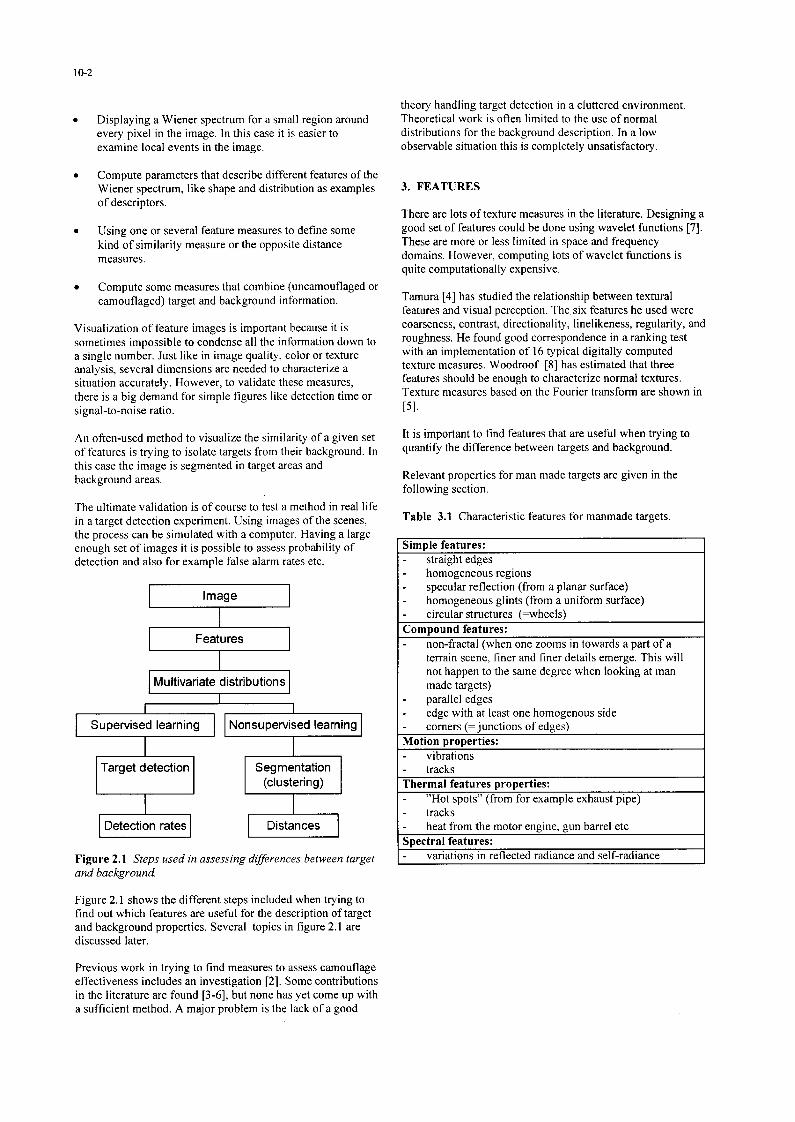
Figure 2.1 Steps used in assessing differences between target and background.
Figure 2.1 shows the different steps included when trying to find out which features are useful for the description of target and background properties. Several topics in figure 2.1 are discussed later.
theory handling target detection in a cluttered environment. Theoretical work is often limited to the use of normal distributions for the background description. In a low observable situation this is completely unsatisfactory.
3. FEATURES
There are lots of texture measures in the literature. Designing a good set of features could be done using wavelet functions [7]. These are more or less limited in space and frequency domains. However, computing lots of wavelet functions is quite computationally expensive.
Tamura [4] has studied the relationship between textural features and visual perception. The six features he used were coarseness, contrast, directionality, linelikeness, regularity, and roughness. He found good correspondence in a ranking test with an implementation of 16 typical digitally computed texture measures. Woodroof [S] has estimated that three features should be enough to characterize normal textures. Texture measures based on the Fourier transform are shown in 151.
It is important to find features that are useful when trying to quantify the difference between targets and background.
Relevant properties for man made targets are given in the following section.
Table 3.1 Characteristic features for manmade targets.
I Simule features: I - straight edges - homogeneous regions - specular reflection (from a planar surface) - homogeneous glints (from a uniform surface) - circular structures (=wheels)
1 Comnound features: - non-fractal (when one zooms in towards a part of a
terrain scene, finer and finer details emerge. This will not happen to the same degree when looking at man made targets)
- parallel edges - edge with at least one homogenous side - corners (= iunctions of edges)
1 Motion aroDerties: I - vibrations I- tracks Thermal features properties: - “Hot spots” (from for example exhaust pipe) - tracks - heat from the motor engine, gun barrel etc Snectral features: . - variations in reflected radiance and self-radiance
Previous work in trying to find measures to assess camouflage effectiveness includes an investigation [2]. Some contributions in the literature are found [3-61, but none has yet come up with a sufficient method. A major problem is the lack of a good
lo-3
Table 3.2 Characteristic features for natural background.
Terrain background (texture features): - coarseness - contrast - directionality - linelikeness - regularity - roughness Others: - Fractal (when one zooms in towards a part of a terrain
scene, finer and finer details emerge ) - non-stationary properties
Several features can be computed. Which features are useful to compute will be addressed later. About half of the features are based on image primitives like edges and blobs, that characterize targets. When computing these features the image is first for every pixel treated with an operator. The resulting image is then processed by a lowpass filter or something similar. This is done to find properties like concentrations of edges per region. For the background features, a local Wiener spectrum is computed for a region centered at each pixel. To save computation time, it is not necessary to compute the Wiener spectrum at every pixel. A coarse grid complemented with interpolation is adequate in most cases. In general, a good estimate is obtained if the grid separation is one fourth of the region size. When computing most of the features, a masking function may be applied to each local region to avoid boundary effects. It corresponds to an aperture function often used in spectral estimation. Here we use a very simple one, the Gaussian.
3.1 Target related features
The target related features used are: mean value, standard deviation, edge concentration, blob concentration, spoke maximum and edge coherence.
Although being first order statistics the mean value (mean) and standard deviation (dev) are included as they correspond to often used measures.
Figure 3.1 The inner and outer mask usedfor computation of the blob concentration.
The blob operator (blob) is defined with the help of figure 3.1. The mean values for the inner window and the outer window are computed and the difference is used as feature value if it exceeds a certain low threshold. Due to the sharp boundaries of these windows, the blob operator has to be applied to every pixel in the input image. As a texture measure for the local region, the mean value of the operator output is computed in the region.
The edge concentration (edgeconc) measure is the number of edge pixels in a local region around the center pixel. Edge- based texture measures have been investigated by Pietikainen and Rosenfeld [9]
The spoke operator (spokemax), as described in [lo], is shown in figure 3.2. It consists of eight spokes and is applied to every pixel in the image. Based on in how many spokes an edge segment is present. as represented in figure 3.2 by an arc, the presence of a small circular object may be detected. The output is an image where the pixel value corresponds to the number of hits that occur. Eight hits indicates a more or less closed curve, while three or four hits may indicate a corner. Instead of computing the mean value, the maximum value for each local region is computed.
K--h / \
Figure 3.2 The spoke opera&.
The implementation of the edge coherence (edgecoh) follows the method given in [ 1 I]. Other work in the same direction includes [ 12,131. Its purpose is to indicate close parallel edges. Like the edge concentration feature, the edge image is used as input. Instead of summing the edge pixels for any direction, here only edges lying along the principal direction are summed. If the direction for an edge element differs from the principal direction it is weighted with respect to the difference in direction. If the edge magnitude is denoted mugn then the edge coherence is computed according to,
edgecoh = (mugnc - csumt)jcsumn
where magnc = edge image value in the center of the region
csumt = c( magn cos( dird?ff ))
csumn = C (map)
and dirdiff= difference in direction between the center pixel and the others.
3.2 Background related features
The background features are all based on. the Wiener spectrum, which is the squared magnitude of the local Fourier transform, and is called power spectrum in signal processing. They are isotropy, autocorrelation length, fractal dimension, directional autocorrelation, main direction, shape. low, medium and high frequency band energy, angular deviation, angular entropy and Fourier transform energy.
lo-4
Given the spatial frequenciesf,,f, and the Wiener spectrum magnitude mug+& the isotropy is defined as in [ 141
isotropy = 255. ~sumu - sumv~
(sum24 + sumvy - 4 sumuvz
where SZWIU =&* .MCl’gn, ,“)
sumv ‘=C(fY \ magnfx Jy J
sumuv = C c
f, fV magn ,xx, ,. Y 1
When computing the autocorrelation length. basically the Wiener spectrum is integrated in the angular dimension. Only the frequency magnitude& of the spatial frequency is used. The feature is defined as
autocorr = 10.0 ’ f,,, . ;msum: fsum
where
msum = C magn f*Jy
fsum = 1 fxf, .magnI. ( f
XT y 1
JJY = Nyquist frequency (=half the sampling rate)
Fractal geometry is a popular area for describing terrain and landscape. In addition, fractal dimension and lacunarity are two properties that can be computed [ 151. Fractals for texture analysis have been studied by Garding [ 161 and others. The Wiener spectrum is again treated as a function of the magnitude of the frequency. The fractal dimension is estimated from the Wiener spectrum magnitude using a least square tit of an angular integrated Wiener spectrum.
The lacunarity @-acterr) represents the amount of deviation an image exhibits from being fractal. Here it is a measure of how good a line will fit to the angular integrated Wiener spectrum.
The three features directional autocorrelation (dirautoc), mean direction (eigenmean) and shape (shape) are computed using a mass model of the Wiener spectrum and computing the inertia ellipsoid. The latter is computed by solving the eigenvalue problem
A.I--/I./4 =o
where A = covariance matrix with components a,,, Here the Wiener spectrum is used as a distribution function,
Solving the eigenvalue equation gives two roots, hi and h2 which correspond to the major and minor radius of the inertia ellipsoid.
The directional autocorrelation feature is defined as
dirautoc = const I,
The main direction is defined as the direction of the principal axis of the inertia ellipsoid.
The shape feature corresponds to the elongeness of the inertia ellipsoid and is defined as the ratio between the minor and the major radius
The next three texture measures, low, medium and high frequency band energy are probably the most relevant features when the problem is to characterize the scale of a pattern. The Wiener spectrum is summed in three different frequency bands. If the Nyquist frequency is&, then the frequency limits are
lowband: 0 toJ,J4
midband: 1;,y/4 -r;,J;!
highband:&/ -j&
Figure 3.3 shows the summation areas.
Figure 3.3 Summation areas when computing Lowband, Midband and Highband.
The total Fourier transform energy is simply defined as
fteneray = k. magnsum
where k is a constant and magnsum = c log(magn + I), log(dc)
magn = Wiener spectrum magnitude,
dc = magnitude at zero frequency
A high value in ftenergy means that the image has a high degree of variation. Knowing that the Wiener spectrum often falls of very rapidly with frequency, the use of logarithms gives high frequencies more weight.
10-5
3.3 Feature examples
Figure 3.4 shows an image divided into square grids of local regions and the corresponding Wiener spectra. Normally the regions are highly overlapped, with a center distance of one or two pixels.
Figure 3.4 Local spectra for a typical image. From left: the input image divided into the regions and the local spectra.
The different background features relate to properties of these spectra. A few examples of feature images are given in figure 3.5
Figure 3.5 An image (upper lef), isotropy (upper right), autocorrelation length (lower lefo and medium frequency band (lower right).
4. DISTANCE MEASURES
We want to be able to express the difference between two areas as a distance using a space defined by some of the previously described features. The distance measures, see [2,2 I], have different underlying assumptions concerning the feature distribution. If mean values and standard deviations are used to characterize a feature, the distribution is normally assumed to be Gaussian and the features are assumed to be independent. Some distances used fall in this class. The reason for this is the simplifications made when applying them in practice. By using the covariance matrix, dependent features can be handled and the Mahalanobis distance is an example of this class. The Wilks measure uses no assumptions.
Because of a high degree of correlation between the different measures, it is advantageous to use distance measures that do not assume independent variables. Using this assumption leads to incorrect results.
Often it is of interest to use well-known quantities that have been used for a long time. One such measure is the signal-to- noise ratio (SNR) which is very common in connection with electrical signals. It is not easy to define an useful SNR for images, but attempts have been made by many researchers.
The different distance measures may be divided into three groups depending on how an area for target or background, is characterized. Most common is to use mean value and standard deviation.
Some measures take explicit consideration to dependent features. The Mahalanobis distance uses the covariance matrix to characterize one area and uses a feature point for the other. The original formulation of the Bhattacharrya measure makes no assumption about the target and background statistics, but often an approximation is used, where the distributions are assumed to be Gaussian and separable. The Wilks measure is a measure of similarity, which make no assumptions.
In table 4.1 the different measures used are listed.
Table 4.1 Listing of several distance measures.
# Distance Comments 1 Wilks Parameter free 2 Bhattacharrya May be parameter free 3 Mahalanobis Uses the covariance matrix 4 Yaki 5 Disabs 6 Dissar
Only mean values Onlv mean values
I
71 L I i
Tsnr I 8 dT-sum 9 dT_suma 10 dT rss 11 1 dT-rss4 12 I Thvle I _- - -, -- 13 Doyle-mod 14 Doyle-log 15 Doyle hybrid
Includes a constant Includes a constant Includes a constant
4.1 The distances
4.1.1 Wk.9 The following description is given by Liu and Jernigan [14]. Let xi@ be the i:th feature value for the k:th sample of class g, where i = 1,2,. ,m and m = the number of extracted features; g=l,2,. .;G (G classes) and k=l,2,. .,np (number of samples in class g). N = C nR is the total number of samples. The Wilks statistic is a measure of class separability that depends on within class and between class scatter matrices. The within class scatter matrix, IV. and between class scatter matrix, B, are defined as
and
10-6
B = [b,] > I,,XN,
where
w,, = f 2 (Xigk g=I k=l
and
- >( -
Xii: ’ i.xk - x jg -
b,, = i n p (Xix - x, )( iYin - xi ) g=I
x,I: and 5, are the mean value of class g and the total sample
mean value for the i’th feature
The sum of within and between class scatter is the total scatter matrix T
tj,=g 2 (X,*,k-X,)(X,++ &!=I k=l
The Wilks statistics is the ratio of within class scatter to total
scatter; IJ = lI+T1
4. I .2. Bhattacharrya This is a measure of the overlap between two normalized distributions. If the distributions aref(x) and g(x), the Bhattacharrya coefficient b,, is defined as [ 171.
This quantity is related to false alarms and false detections.
In one implementation the features from the two regions to be compared are assumed to be Gaussian with mean values ,u,, pl and standard deviations oi, 02. Assuming independent features gives the sum of the Bhattacharrya distance for the features between the two areas 1 and 2. Defining b as -log(b,,& gives
b = lN.c ,uor
Here x is the feature for a point in the image and the feature for rest of the image is characterized by the mean value p and the covariance matrix C. Sometimes a small target area is compared with a larger background. In this case the target area statistics is approximated by its mean value and used for x in the expression above.
4.1.4. Yaki This measure was designed by Yakimovski [19] in order to find out whether two regions are of the same kind or not. He found a measure, here called yaki for simplicity, that is for one feature given by
2
yaki= o** ,‘(T, ‘02 ( > where 0,z = standard deviation of the feature in the union of
region 1 and region 2 oi= standard deviation of the feature in region 1 02= standard deviation of the feature in region 2 Assuming Gaussian models for the two regions with mean values of p, and ,~r, and standard deviations of IS, and o2 then the above expression may be evaluated to give
Yaki,,, =I+ (4 -d ] h-4
(4.(T, .a,) (2.C3 .cQ)
Sometimes the constant 1 in the above expression is neglected in order to make the yaki measure look like a signal-to-noise ratio. If several independent features are used this measure will be given by
yaki = c yakif,,,, where yak&, is computed for each feature according to equation above.
4.1.5. T-Student snr In one application there was a need for simple measures that were fast to compute and has similarities to simple known measures, in this case the signal-to-noise ratio. The T-Student test [52] is used to see if two distributions are similar. We define it as
Using mean values and standard deviations means that the underlying distributions are assumed to be normal.
4. I 6. Disabs
Disabs = 1 N *
where the summation is done over all the features used. 4. I. 7 Dissqr
4.1.3 Mahalanobis distance This distance often occurs in connection with normal distributions. It is a measure from one point in a distribution to the center of the distribution. It is defined as [IS].
10-7
4. I. 9. dT-rss4
r----- dT_rss4= 1 ;F* // + )
2 T-PB +4.02T
1 F‘vrw‘ I
4.1.13. doymod
doyle-mod = 1 jx l :‘Zjlui-rr)‘+~*dT-~8)‘)
where k=0.4 12.
4.1.14. doylog I I
where k=0.00477.
4.1.15. doyhyb
doyle-hybrid = i ;G* \j C [(hI(,,Ul)-ln(,UR)) i+k+I.-~B)2) F.u,,wcr
where k=0.000023.
4.4. Examples
An example of distance computation is shown in Figure 4.1 The distances are chosen in an earlier experiment.
Since many measures are used in the comparisons in a later part they will be defined here. The order here is in no way indicating their relevance.
Other examples of distance computations are given in section 5and6.
5. EXPERIMENTS WITH THE SEARCH-2 IMAGE DATA SET
44 images from the Search2 data set [20] have been used in some experiments trying to correlate the distances from several distance measures with perceptual measures on detection time and hits performance. The images were limited in field-of- view to have a size of 256*256 pixels. They were selected with a magnification such that the target width occupied around 25 to 50 pixels. 5 images are from the Bl set, 26 from the B4 set and 13 from the B 16 set. The tables in this section summarize experiments using several features and several distance measures. In several cases an exhaustive search has been performed to find the highest correlation with the perception data. Ideally, a model would be derived beforehand, to limit the search to relevant cases.
Mahalanobis 2.5
Bhattacharrya 0.6 Yakimowski 0.8
Table 5.1. Correlation between distance and detection time.
Dirautoc, isotropy dTsuma 3 features 1 Edgecoh. dirautoc, dTsum 0.756
isotrony 2 Edgecoh, &energy dT-rss4 0.728
isotropy Dirautoc, isotropy, dT-rss medfreq
3 Dirautoc, isotropy, dTsuma 0.708 lowfreq
The three best are shown, just to indicate that there is no big difference between the good ones in each experiment. Using several features gives a better result but the risk is to adjust to the current image data set too much. In table 5.1 and 5.2 the distances are correlated with the detection times. Some experimentation showed that correlation with the inverse of the distances gave a somewhat better result. The corresponding results are shown in table 5.3 and 5.4. A nonlinear function may be used, but again an adjustment to the current data set has to be avoided. The correlation is given with three decimals in the tables just to indicate small differences. In practise only the first decimal may be relevant.
Figure 4.1 Distance computation using the isotropy and autocorrelation length. The inner area outlines the target area. The background area is defined as the area between the inner and outer square.
10-8
5.1. Comments Table 5.2. Correlation between inverse distance and detection time. Rank 1 Features 1 Distance 1 Correlation 1 The tests indicate that the best result will be obtained using
mean and variance based distances. Also it is evident that the inverse distance gives a better correlation reaching up to 0.85 in some case. The different tests also indicate that the features isotropy and dirautoc are among the best to use. If a third feature will be used, then ftenergy is a natural choice. One reason that isotropy is good is that it reacts to small straight edge segments that are common on targets but unusual in the background.
Better results may perhaps be obtained if the whole scene is processed. Now there is no estimation of possible false alarms outside the small background area used.
3 1 Dirautoc, edgecoh, 1 doyle ( 0.857 6. APPLICATION TO CAMOUFLAGE ASSESSMENT isotropy Dirautoc, isotropy, dissqr mean
Figure 6.1 shows a sequence of images where the targets are more and more camouflaged (simulated here by lowering the target contrast). The features used are directional autocorrelation distance (dirautoc) and isotropy. In the scatter image to the right of the image the covariance ellipses for the target area are plotted
Table 5.3. Correlation between distance and hits. Rank Features Distance Correlation 1 feature 1. Ftenerav dT rss4 0.612
Figure 6!1 A sequence of images where the targets are more and more camouflaged (simulated here by lowering the target contrast). To the right of the images scatter plots are shown with covariance ellipses for the target area and background area.
10-9
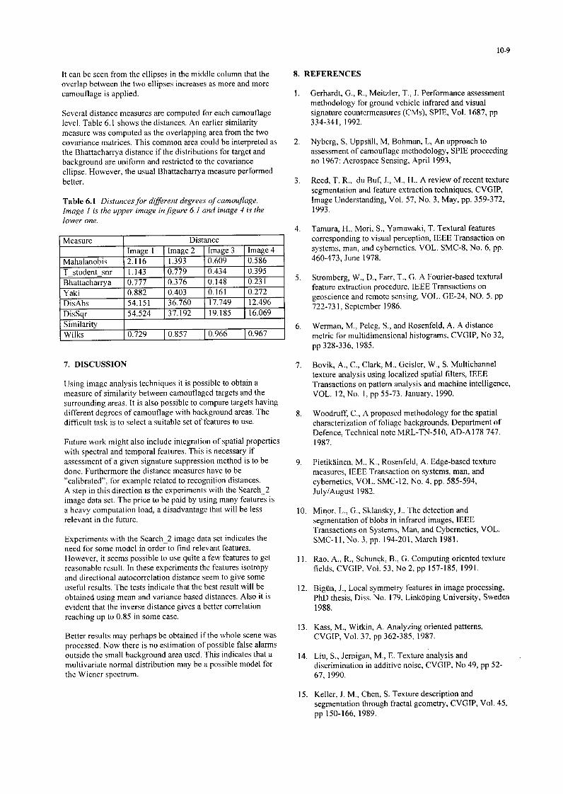
It can be seen from the ellipses in the middle column that the overlap between the two ellipses increases as more and more camouflage is applied.
Several distance measures are computed for each camouflage level. Table 6.1 shows the distances. An earlier similarity measure was computed as the overlapping area from the two covariance matrices. This common area could be interpreted as the Bhattacharrya distance if the distributions for target and background are uniform and restricted to the covariance ellipse. However, the usual Bhattacharrya measure performed better.
Table 6.1 Distancesfor different degrees of camouflage. Image I is the upper image in figure 6. I and image 4 is the lower one.
7. DISCUSSION
Using image analysis techniques it is possible to obtain a measure of similarity between camouflaged targets and the surrounding areas, It is also possible to compare targets having different degrees of camouflage with background areas. The difficult task is to select a suitable set of features to use.
Future work might also include integration of spatial properties with spectral and temporal features. This is necessary if assessment of a given signature suppression method is to be done. Furthermore the distance measures have to be “calibrated”, for example related to recognition distances. A step in this direction is the experiments with the Search-2 image data set. The price to be paid by using many features is a heavy computation load, a disadvantage that will be less relevant in the future.
Experiments with the Search-2 image data set indicates the need for some model in order to find relevant features. However, it seems possible to use quite a few features to get reasonable result. In these experiments the features isotropy and directional autocorrelation distance seem to give some useful results. The tests indicate that the best result will be obtained using mean and variance based distances. Also it is evident that the inverse distance gives a better correlation reaching up to 0.85 in some case.
Better results may perhaps be obtained if the whole scene was processed. Now there is no estimation of possible false alarms outside the small background area used. This indicates that a multivariate normal distribution may be a possible model for the Wiener spectrum.
8. REFERENCES
1.
2.
3.
4.
5.
6.
7.
8.
9.
10.
11.
12.
13.
14.
15
Gerhardt, G., R., Meitzler, T., J. Performance assessment methodology for ground vehicle infrared and visual signature countermeasures (CMs), SPIE, Vol. 1687, pp 334-341, 1992.
Nyberg, S, Uppsall, M, Bohman, L, An approach to assessment of camouflage methodology, SPIE proceeding no 1967: Aerospace Sensing, April 1993,
Reed, T. R., du Buf, J., M., H.. A review of recent texture segmentation and feature extraction techniques, CVGIP, Image Understanding, Vol. 57, No. 3, May, pp. 359-372, 1993.
Tamura, H., Mori, S., Yamawaki, T. Textural features corresponding to visual perception, IEEE Transaction on systems, man, and cybernetics, VOL. SMC-8, No. 6, pp. 460-473, June 1978.
Stromberg, W., D., Farr, T., G. A Fourier-based textural feature extraction procedure, IEEE Transactions on geoscience and remote sensing, VOL. GE-24, NO. 5. pp 722-73 1, September 1986.
Werman, M., Peleg, S., and Rosenfeld, A. A distance metric for multidimensional histograms, CVGIP, No 32, pp 328-336, 1985.
Bovik, A., C., Clark, M., Geisler, W., S. Multichannel texture analysis using localized spatial filters, IEEE Transactions on pattern analysis and machine intelligence, VOL. 12, No. 1, pp 55-73, January, 1990.
Woodruff, C., A proposed methodology for the spatial characterization of foliage backgrounds, Department of Defence, Technical note MRL-TN-5 10, AD-Al 78 747, 1987.
Pietikainen, M.. K., Rosenfeld, A. Edge-based texture measures, IEEE Transaction on systems, man, and cybernetics, VOL. SMC-I 2, No. 4, pp. 585-594, July/August 1982.
Minor, L., G., Sklansky, J., The detection and segmentation of blobs in infrared images, IEEE Transactions on Systems, Man, and Cybernetics, VOL. SMC-11, No. 3, pp. 194-201, March 1981.
Rao, A., R., Schunck, B., G. Computing oriented texture fields, CVGIP, Vol. 53, No 2, pp 157-185, 1991.
Bigtin, J., Local symmetry features in image processing, PhD thesis, Diss. No. 179, Linkiiping University, Sweden 1988.
Kass, M., Witkin, A. Analyzing oriented patterns, CVGIP, Vol. 37, pp 362-385, 1987.
Liu, S., Jernigan, M., E. Texture analysis and discrimination in additive noise, CVGIP, No 49, pp 52- 67, 1990.
Keller, J. M., Chen, S. Texture description and segmentation through fractal geometry, CVGIP, Vol. 45, DD 150-166, 1989.
10-10
16. Garding, J. A note on the application of fractals in image analysis, Proceedings of SSAB (Swedish Society for Automated Image Analysis, Lund, Sweden, pages 80-83, 1988.
17. Duda, R., Hart, P., Pattern classification and scene analysis, John Wiley & Sons, p 40, New York, 1973.
18. Duda, R., Hart, P., Pattern classification and scene analysis, John Wiley & Sons, p 24, New York, 1973.
19. Schachter, B., J., A survey and evaluation of flir target detection/segmentation algorithms, pp 49-57, AD-Al20 072, 1983.
20. Toet, A., Bijl, P., Kooi, F.L., Valeton, J.M., A high- resolution image data set for testing search and detection models, TNO-report TM-98-A020, April 1998.
21. Copeland, A., C., Trivedi, M., M., McManamey, J., R., Evaluation of image metrics for target discrimination using psychophysical experiments, Opt. Eng. 35(6), pp 1714-1722, June 1996.


![OPTICS] Optical Camouflage - Electronics Makerelectronicsmaker.com/em/admin/pdfs/free/Optical.pdfoptical camouflage is a part of Active camouflage (or Adaptive camouflage) is a group](https://static.documents.pub/doc/80x56/5f01e08f7e708231d40178cf/optics-optical-camouflage-electronics-m-optical-camouflage-is-a-part-of-active.jpg)


