Assessing Hedge Fund Performance with Institutional Constraints Marat Molyboga Efficient Capital Management, LLC Seungho Baek * Murray Koppelman School of Business, City University of New York John F. O. Bilson Stuart School of Business, Illinois Institute of Technology Abstract Standard tests for anomalies in hedge fund returns are not consistent with investment practices because they ignore performance reporting delay, overlook fund selection standards of institu- tional investors, and often use portfolios with too many funds. This paper introduces a set of tests based on a large scale simulation framework and stochastic dominance methodology. These tests incorporate constraints that are standard practice in the institutional investment field. We investigate momentum in performance of hedge funds in the managed futures industry consid- ering these constraints. From various tests based on the simulation, we find the evidence of the performance persistence in the institutional investment areas. Keywords: Hedge Funds, Commodity Trading Advisors, Performance Persistence, Institutional Investment JEL: : G11; G12; G23 1. INTRODUCTION Momentum is regarded as a market anomaly that has been observed in various financial mar- kets. Cross-sectional momentum in returns has been documented in US equities (Jagadeesh and Titman, 1993; Fama and French, 1996), international equity markets (Rouwenhorst, 1998), in- dustries (Moskowitz and Grinblatt, 1999) and equity indices (Asness et al., 1997), Bhojraj and Swaminathan, 2006). Momentum in returns is present in foreign exchange (Shleifer and Sum- mers, 1990) and commodities markets (Erb and Harvey,2006, Gorton et al., 2013). Asness et al. (2013) analyze cross-sectional momentum and value strategies across several asset classes including individual stocks, stock indices, currencies, commodities and bonds. They find signif- icant momentum in every asset class considered in their studies. * Corresponding author, Address: 2900 Bedford Ave, Brooklyn, NY 11210, USA. Tel.: +1 718 951 5154; Fax: +1 718 951 4385 Email addresses: [email protected](Marat Molyboga), [email protected](Seungho Baek), [email protected](John F. O. Bilson)
Transcript
Assessing Hedge Fund Performance with Institutional Constraints
Marat Molyboga
Efficient Capital Management, LLC
Seungho Baek∗
Murray Koppelman School of Business, City University of New York
John F. O. Bilson
Stuart School of Business, Illinois Institute of Technology
Abstract
Standard tests for anomalies in hedge fund returns are not consistent with investment practicesbecause they ignore performance reporting delay, overlook fund selection standards of institu-tional investors, and often use portfolios with too many funds. This paper introduces a set oftests based on a large scale simulation framework and stochastic dominance methodology. Thesetests incorporate constraints that are standard practice in the institutional investment field. Weinvestigate momentum in performance of hedge funds in the managed futures industry consid-ering these constraints. From various tests based on the simulation, we find the evidence of theperformance persistence in the institutional investment areas.
Momentum is regarded as a market anomaly that has been observed in various financial mar-kets. Cross-sectional momentum in returns has been documented in US equities (Jagadeesh andTitman, 1993; Fama and French, 1996), international equity markets (Rouwenhorst, 1998), in-dustries (Moskowitz and Grinblatt, 1999) and equity indices (Asness et al., 1997), Bhojraj andSwaminathan, 2006). Momentum in returns is present in foreign exchange (Shleifer and Sum-mers, 1990) and commodities markets (Erb and Harvey,2006, Gorton et al., 2013). Asness etal. (2013) analyze cross-sectional momentum and value strategies across several asset classesincluding individual stocks, stock indices, currencies, commodities and bonds. They find signif-icant momentum in every asset class considered in their studies.
∗Corresponding author, Address: 2900 Bedford Ave, Brooklyn, NY 11210, USA. Tel.: +1 718 951 5154; Fax: +1718 951 4385
In mutual funds and hedge funds, momentum is regarded as the effect of anomalies. Hen-dricks et al. (1993) test for momentum in mutual fund returns. They find persistence in rel-ative performance of mutual funds with the difference in the risk-adjusted performance of thetop and bottom octile portfolios of six to eight percent per year. Carhart (1997) uses decilemethodology to evaluate persistence in mutual fund performance. He finds strong persistence inperformance of the worst performing managers and no evidence of skilled or informed mutualfund portfolio managers who consistently provide better risk-adjusted returns. Agarwal and Naik(2000a, 2000b) document significant quarterly persistence of hedge fund returns primarily drivenby the worst performing funds. Capocci and Hubner (2004) use decile methodology to discoverlack of persistence among the top and bottom decile funds and little persistence among middledecile funds.
Kosowski et al. (2007) apply a Bayesian estimate of Jenson alphas (Jenson, 1968), intro-duced by Pastor and Stambaugh (2002), to demonstrate performance persistence over a one-yearhorizon. Jagannathan et al. (2010) use weighted least squared and GMM approaches to findsignificant performance persistence among the top performing hedge funds and little evidence ofpersistence among the bottom performing funds. They rank funds using the t-statistic of alphaand report superior performance of portfolios of all funds in the top decile and the top tercile todemonstrate the practical importance of their approach for institutional investors.
The techniques used to test for momentum in various asset classes and mutual funds areoften relevant to institutional investors, who can relatively easily build large long-short portfoliosof winners-losers and rebalance them monthly, although these investors still need to deal withpractical implementation issues of transaction costs and market impact. Similar techniques areused to evaluate persistence in performance of hedge funds. However, these techniques cannotbe implemented by prudent institutional investors because the methodology ignores the delayin hedge fund reporting and, therefore, investment recommendations are based on informationthat is not available at the time of investment decisions. In addition, the studies consider fundsthat have assets under management that are too small for institutional investors, have very shorttrack records (sometimes as little as 12 months) and involve portfolios with too many funds bepractically investable. The failure to account for these common industry constraints may limitthe applicability of the academic research to actual investment practice.
The objective of this paper is to examine the issue of performance persistence within a frame-work that incorporates common industry constraints by institutional investors when creating andrebalancing portfolios of hedge funds. These constraints serve to reduce transaction costs overmultiple periods and include limitations on individual funds: the size of assets under manage-ment and the length of the fund track record. The approach also places a limit on the numberof funds to be included in the portfolio and on the turnover of these funds. Specifically, ourmodel assumes that the institutional investor selects a discrete number of otherwise acceptablefunds and that, once selected, a fund will stay in the portfolio until it no longer satisfies the se-lection criteria. The imposition of these constraints results in a very large number of feasibleportfolios in each period. The model employs a large scale simulation framework designed totest for anomalies in hedge fund returns in a way that is consistent with requirements of largeinstitutional investors.
Little work has been done in investigating performance persistence among Commodity Trad-ing Advisors (CTAs), a subset of hedge funds that is primarily known for utilizing trend-followingor time-series momentum strategies in futures and options markets. Institutional interest in CTAshas increased in response to the performance of these funds during the Global Financial Crisiswith assets growing from US $131 billion in 2005 to US $330 billion in the first quarter of 2015
2
according to BarclayHedge Group. The simulation model provides a test for persistence in CTAperformance that could be used by institutional investors who are interested in allocating to thissegment of the alternative investments space. The model incorporates two important constraints.First, it excludes funds who are in the bottom 30% in assets under management or whose trackrecord is fewer than 60 months old. Second, the performance of the remaining funds is measuredby calculating the t-statistic of alpha with respect to the CTA benchmark using data from theprevious 60 months. In the first month, the model creates an initial portfolio by selecting 20funds from the top quintile of the performance distribution and also randomly selects another 20funds from the entire sample. In each subsequent month, funds that liquidate or fail to meet theselection criteria are randomly replaced from the pool of funds that meet the corresponding selec-tion criteria. A single observation consists of a time-series returns over the entire out-of-sampleperiod from 1999 to 2013. The simulation engine repeats this procedure 10,000 times and thencompares the performance of the strategy applied to all funds to the strategy that only considersfunds in the top quintile. The dataset contains 4,909 funds over the period 1994 through 2013.We show that the strategy of selecting top quintile funds significantly improves risk-adjustedperformance of hypothetical portfolios of institutional investors in out-of-sample. We performrobustness analysis to evaluate robustness of our findings across different market environments.
The evaluation of out-of-sample results is challenging primarily because simulation resultsare not independent since the returns of the same funds are used across many simulation; there-fore, standard statistical tests are inappropriate. The model employs a bootstrapping procedure toapproximate the sampling properties of the test results. The comparison is based upon stochas-tic dominance (SD) methodology, developed by Hanoch and Levy (1969), Hadar and Russell(1969), and Rothschild and Stiglitz (1971), has been used in both decision theory with uncer-tainty and used as an alternative to mean-variance analysis to evaluate portfolios (Levy and Sar-nat, 1970). As Fischmar and Peters (1991) describe, stochastic dominance is a comprehensivemeasure of portfolio return and risk in that, unlike mean-variance analysis which only considersmean and variance, it utilizes the entire distributions of returns to compare benefits of variousportfolios to a broad set of investors without having to make assumptions about each investor’sutility function. Second order stochastic dominance is particularly attractive because it highlightsthe situations when all risk averse investors would agree that one distribution is better than theother.
The rest of the paper is organized as follows. Section 2 describes the data and treatment foreliminating biases; Section 3 discusses the methodologies used in the performance persistenceliterature, introduces the large scale simulation framework as a an alternative methodology and astochastic dominance framework used to evaluate out-of-sample performance; Section 4 presentsempirical results and Section 5 includes concluding remarks.
2. Data
This study is based upon the Barclay Hedge database, the largest publicly available databaseof Commodity Trading Advisors. Joenvaara et al. (2012) compare five databases (BarclayHedge,TASS, HFR, Eurekahedge and Morningstar) and find that BarclayHedge has the largest numberof funds (10,520), compared to 8,788 funds in the TASS data base. Buraschi et al. (2014)summarizes two advantages of the usage of BarclayHedge database. The first advantage is thisdatabase is least likely to be affected by survivorship bias because it includes the largest numberof active funds and dead funds. The second one is that it has the longest asset under management(AUM) history and the fewest missing values of AUM.
3
Diz (1999), Gregoriou et al.(2005), Molyboga et al. (2014), and Bhardwaj et al.(2014) doc-ument backfill/incubation, liquidation and survivorship biases in CTA databases.1 They provideevidence that these biases can skew results of CTA performance persistence, suggesting the im-portance of appropriately adjusting for biases in CTA performance persistence studies.
The database includes 4,909 active and defunct funds over the period between Decemberof 1991 and December of 2013 with the out-of-sample period between January of 1999 andDecember of 2013. Multi-advisors funds are removed from the analysis because they are outsideof our research scope2. Funds with the peak value of AUM under US$ 10 million are eliminatedbecause they are too small. institutional investors often have provisions that prevent them fromrepresenting more than 50% of AUM of any fund. These small funds also tend to have lowerquality returns. Finally, the sample only includes funds that report returns net-of-fees to ensurecomparability of returns.
The data filtering procedure accounts for survivorship, backfill/incubation and liquidationbiases that are common for CTA and hedge fund databases. The survivorship bias is straight-forward to address. The sample includes the graveyard database that contains defunct funds toaccount for the survivorship bias. But backfill and incubation biases are more difficult to address.Backfill and incubation biases typically arise from the voluntary nature of self-reporting. Fundsusually go through an incubation period during which they build a track record using proprietarycapital. If the fund’s track record is attractive, then fund managers will choose to start reportingto a database to raise capital from outside investors and backfill the returns generated prior totheir inclusion in the database. Since funds with poor performance are unlikely to report theirreturns to the database, this results in the incubation/backfill bias. Aragon and Nanda (2014)highlight significant differences in reporting and disclosures requirements for mutual funds andhedge funds. Corporate managers have limited discretion in the timing and quality of informa-tion release due to strict requirements of the U.S. Securities and Exchange Commission (SEC),GAAP and stock exchanges. In contrast, hedge funds managers are free to set their own dis-closure policies when they report to public databases. Mutual funds must register with the SECand are subject to regulations intended to protect investors (Securities Act of 1933; SecuritiesAct of 1934; the investment company Act of 1940; the Investment Advisers Act). Unlike mutualfunds, hedge funds are not required to register with the SEC and provide performance informa-tion. Malkiel and Saha (2005) suggest that the regulatory reporting requirements and audits bythe regulators significantly reduce the backfill bias in mutual fund returns whereas hedge fundsare able to strategically delay reporting to public databases which introduces a backfill bias inreturns.
This study uses two approaches to mitigate backfill and incubation biases. The first method-ology, suggested by Fama and French (2010), limits the tests to funds that reach US$ 10 millionAUM in 2013. Once a fund passes the AUM minimum, it is included in all subsequent tests toavoid creating selection bias. Unfortunately, many funds, including very successful and estab-lished CTAs, originally reported only net returns for an extended period of time prior to includingAUM data several years later. Using the methodology of Fama and French (2010) exclusivelywould completely eliminate large portions of valuable data for such funds. To include this data,the technique suggested by Kosowski et al. (2007) that eliminates the first 24 months of datafor such funds is applied. The liquidation bias estimate of 1% as suggested in Ackermann et al.
1Bhardwaj et al.(2014) report that survivorship bias is 2.21% for volume weighted and 4.15% for equally weighted,backfill bias is 1.92% for volume weighted and 3.66% for equally weighted
2This study focuses on direct investments of institutional investors in funds whereas multi-advisors are fund of funds.4
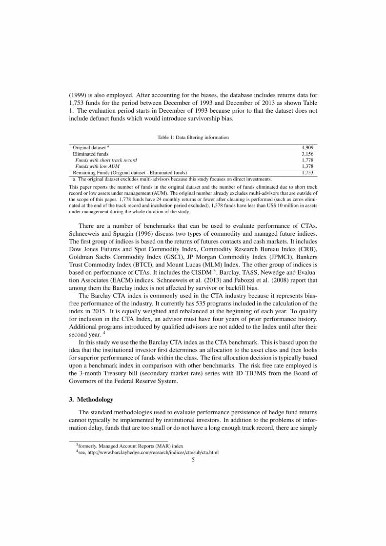
(1999) is also employed. After accounting for the biases, the database includes returns data for1,753 funds for the period between December of 1993 and December of 2013 as shown Table1. The evaluation period starts in December of 1993 because prior to that the dataset does notinclude defunct funds which would introduce survivorship bias.
Table 1: Data filtering information
Original dataset a 4,909Eliminated funds 3,156Funds with short track record 1,778Funds with low AUM 1,378
Remaining Funds (Original dataset - Eliminated funds) 1,753a. The original dataset excludes multi-advisors because this study focuses on direct investments.
This paper reports the number of funds in the original dataset and the number of funds eliminated due to short trackrecord or low assets under management (AUM). The original number already excludes multi-advisors that are outside ofthe scope of this paper. 1,778 funds have 24 monthly returns or fewer after cleaning is performed (such as zeros elimi-nated at the end of the track record and incubation period excluded), 1,378 funds have less than US$ 10 million in assetsunder management during the whole duration of the study.
There are a number of benchmarks that can be used to evaluate performance of CTAs.Schneeweis and Spurgin (1996) discuss two types of commodity and managed future indices.The first group of indices is based on the returns of futures contacts and cash markets. It includesDow Jones Futures and Spot Commodity Index, Commodity Research Bureau Index (CRB),Goldman Sachs Commodity Index (GSCI), JP Morgan Commodity Index (JPMCI), BankersTrust Commodity Index (BTCI), and Mount Lucas (MLM) Index. The other group of indices isbased on performance of CTAs. It includes the CISDM 3, Barclay, TASS, Newedge and Evalua-tion Associates (EACM) indices. Schneeweis et al. (2013) and Fabozzi et al. (2008) report thatamong them the Barclay index is not affected by survivor or backfill bias.
The Barclay CTA index is commonly used in the CTA industry because it represents bias-free performance of the industry. It currently has 535 programs included in the calculation of theindex in 2015. It is equally weighted and rebalanced at the beginning of each year. To qualifyfor inclusion in the CTA Index, an advisor must have four years of prior performance history.Additional programs introduced by qualified advisors are not added to the Index until after theirsecond year. 4
In this study we use the the Barclay CTA index as the CTA benchmark. This is based upon theidea that the institutional investor first determines an allocation to the asset class and then looksfor superior performance of funds within the class. The first allocation decision is typically basedupon a benchmark index in comparison with other benchmarks. The risk free rate employed isthe 3-month Treasury bill (secondary market rate) series with ID TB3MS from the Board ofGovernors of the Federal Reserve System.
3. Methodology
The standard methodologies used to evaluate performance persistence of hedge fund returnscannot typically be implemented by institutional investors. In addition to the problems of infor-mation delay, funds that are too small or do not have a long enough track record, there are simply
too many funds in existence for an institutional investor to consider. The large scale simulationframework incorporates real-life constraints, and the stochastic dominance framework is used toevaluate out-of-sample simulation results. Since simulation results are not independent, a boot-strapping procedure is used to approximate the sampling properties of the test results and allowfor statistical inference.
3.1. Review of performance persistence methodologies and investment practices
Most performance persistence tests are similar to the techniques used to test for cross sec-tional momentum. For example, Asness et al. (2013) perform comprehensive tests for cross-sectional momentum in eight diverse markets and asset classes including individual stocks inthe United States, the United Kingdom, continental Europe, and Japan as well as country eq-uity index futures, government bonds, currencies and commodity futures. As in Jegadeesh andTitman (1993), Fama and French (1996), Grinblatt and Moskowitz (2004), they use the com-mon measure of the past 12-month cumulative raw return on the assets, skipping the most recentmonths return, MOM2-12. The most recent month is typically skipped in the literature to avoidthe one-month reversal in stock returns potentially driven by liquidity and microstructure issues(Jegadeesh, 1990; Lo and MacKinaly, 1990, Boudoukh et al., 1994; Grinblatt and Moskowitz,2004). However, excluding the most recent month of returns is irrelevant in other asset classes be-cause the one-month reversal is insignificant outside of stocks (Asness et al. 2013). The standardapproach is to sort the remaining sample using the momentum measure and track performanceof top third, middle third and bottom third portfolios. The Sharpe ratio and the t-statistic of alphaof the spread between the top and bottom portfolios are used to provide evidence of momentum.Implicitly, this procedure assumes that the investor is long all of the instruments in the top thirdand is short all of the instruments in the bottom third. Further, the instruments included in the topand bottom third may vary on a monthly basis potentially leading to high turnover. Though someother studies use deciles (Jegadeesh and Titman, 1993; Fama and French, 1996) either approachresults in a finding that can be replicated by institutional investors as long as they overcome thepractical challenges of portfolio rebalancing and trading expenses that include transaction costsand market impact. The issues of market impact are explicitly addressed in Korajczyk and Sadka(2004).
Similar techniques are used to evaluate persistence in performance of hedge funds (Capocciand Hubner, 2004; Kosowski et al., 2007, Jagannathan et al., 2010). Though the ranking method-ologies used in the studies are very relevant for fund evaluation, institutional investors cannotdirectly benefit from the findings because i) the studies often ignore the delay in hedge fund re-porting, thus requiring information not available at the time of investment decision, ii) considerfunds that have assets under management that are too small for institutional investors, iii) havevery short track records and iv) involve portfolios with the number of funds that are too large tobe practical.
Examination of hedge fund returns should consider the reporting delay in hedge funds per-formance which is not present in mutual funds 5. However, previous studies ignore the delayin hedge fund reporting (Capocci and Hubner, 2004; Kosowski et al., 2007; Jagannathan et al.,
5Performance of mutual funds can be aggregated quickly because they report their performance daily. In contrast,hedge funds and CTAs report their performance monthly and it often takes several weeks to finalize end-of-month per-formance values.
6
2010) which introduces a look-ahead bias 6. if hedge funds are evaluated on January 1st, onlyreturns through the end of November of the previous year are available in the database and De-cember returns are unavailable until the end of January. In this study, a lag of one month is usedto account for the delay in performance reporting of CTAs.
This article suggests a methodology that accounts for investment practices. In general, thereare no hard rules describing standards of institutional investors but there are several publicationsthat summarize best practices. According to a Greenwich Roundtable report7, institutional in-vestors should avoid relying on a fund’s short term track records because it might overstate afund manager’s skill; while long track records that capture performance across different marketconditions are more likely to provide greater insight into advantages and risks of the manager’sinvestment approach. Therefore, we utilize two minimal requirements that are relevant for in-vestment practices the length of track record and AUM size. However there is not universalagreement on the levels of the minimal requirements. The preceding studies consider funds withtrack records that are too short or very low level of AUM. Capocci and Hubner (2004) considerfunds with any amount of assets under management and as little as 12 months of data. Jagan-nathan et al. (2010) consider funds with any amount of assets under management and the lengthof track record that is potentially as short as 36 months of returns, thus, potentially includingfunds that prudent institutional investors would not consider. Kosowski et al. (2007) requirethe level of assets under management of US$20 million and consider funds with as few as 24months of data but also demonstrate that performance persistence results are not driven by theshort look-back period and small funds by repeating analysis using 36, 48 and 60 months of dataand considering large (above median AUM) and small (below median AUM) funds separately.Although the minimum AUM threshold level of US$20 million eliminates hedge funds with lowlevel of assets under management, it does not account for the substantial growth in assets undermanagement in the hedge fund space. Burghardt and Walls (2004) consider 42 managers with 10years of data and at least US $100 million AUM as examples of established managers who havebeen successful at building their businesses. Barclay CTA index includes advisers with at leastfour years of track record. Since there are no hard rules, we apply reasonable requirements forthe length of track record and AUM. We require the track record of 60 months which seems to besufficient to draw inferences about fund manager’s skill but not too long to be overly restrictive.We utilize a dynamic AUM approach that reflects the dynamic nature of the industry size andexcludes the smallest 30 percent of fund managers based on their AUM to focus on the managersthat are large enough for institutional investors.
Institutional investors can hold highly diversified portfolios of mutual funds, but that ap-proach is not practical with hedge fund investments due to higher minimum investment require-ments and significant oversight cost relative to marginal portfolio benefit. While mutual fundshave low minimum investment requirements (around US$1,000 or less than US $1,000) to openan account and no minimum for additional subscription amounts, hedge funds require signif-icantly higher minimum investments. Moreover, the Investment Company Act of 1940 limitsinvestments in hedge funds to investors with at least US $5 million in investments to protect un-sophisticated investors 8. The preceding studies consider performance of decile or trecile hedge
6The most notable example of adjusting for data availability in academic research is the accounting book value indefinition of book-to-market used in Fama-French (1992). They suggest utilizing a 6-month lag which is sufficient toaccount for delay in accounting reporting.
7see, Best Practices in Alternative Investing: Due Diligence (2010) available athttp : //www.greenwichroundtable.org/system/files/BP − 2010.pdf
8see, http : //www.ici.org/files/faqs hedge7
fund portfolios that include a very large number of funds. Jagannathan et al. (2010) employtrecile portfolios with 252 funds and decile portfolios with 77 funds. Since institutional investorsallocate to a significantly smaller number of funds, that will potentially result in a tracking errorthat is very high. This practical implementation issue is outside of the scope of typical perfor-mance persistence studies. In order to address all the above issues, this paper introduces a largescale simulation framework with real-life constraints that is capable of evaluating fund selectionapproaches in a way that is relevant for institutional investors.
3.2. Large scale simulation frameworkThe large scale simulation framework that we introduce in this paper is designed to evaluate
fund selection approaches with real life constraints. The out-of-sample period is between Jan-uary of 1999 and December of 2013, the longest out-of-sample backtesting period in empiricalresearch of CTAs. The simulation framework uses a lag of one month to account for the delayin performance reporting of CTAs and employs 10,000 simulations. A single simulation runresults in several time-series that represent monthly out-of-sample returns of equally weighted(or equally risk-weighted) portfolios of randomly selected CTAs and CTAs chosen from the topquintile based on the t-statistic of alpha with respect to the CTA benchmark.
3.2.1. Random CTA selectionThe in-sample/out-of-sample framework mimics actions of an institutional investor who
makes allocation decisions at the end of the month.9 The first decision is made in Decem-ber of 1998. Because the delay of CTA reporting, the investor has returns information throughNovember of 1998, the investor considers all funds that have complete set of 60 months of re-turns between December of 1993 and November of 1998. First, the investor eliminates all fundsin the bottom 30 percent of AUM among the funds considered. This relatively AUM thresh-old approach is more appropriate than a fixed AUM approach commonly used in the literature(Kosowski et al., (2007)) because the level of AUM has gone up substantially over the last 15years. Then the investor randomly chooses 20 funds10 from the remaining pool of CTAs andallocates to them either equally notionally (also known as 1/N approach) or equally after ad-justing for volatility approach. Equal notional allocation (hereafter, EN) is not commonly usedin momentum literature, DeMiquel et al. (2009) argue that EN outperforms most variations ofmean-variance optimization in out-of-sample portfolio optimization. Equal volatility adjusted(hereafter, EVA) allocation approach is very similar to EN except that each asset’s weight timesits volatility is the same for each asset in the portfolio, rather than each asset’s weight is the same.Volatility is estimated using sample standard deviations over the previous 60 months, allowingfor a one-month reporting lag. The return of both EN and EVA portfolios is calculated for Jan-uary of 1999 using the liquidation bias adjustment for the funds that liquidate during the month.At the end of January of 1999, the pool of CTAs is updated and defunct constituents of the orig-inal portfolio are randomly replaced with funds from the new pool at which point the portfoliois rebalanced again using EN and EVA approaches. The process is repeated until the end of theout-of-sample period in December of 2013. A single simulation results in two out-of-samplereturn stream between January of 1999 and December of 2013 - one for EN and the other one forEVA approach.
9Though in this paper we use monthly rebalancing which is common in managed futures due to its high liquidity, theframework can be easily modified to account for quarterly, semi-annual or annual rebalancing.
10The number of funds in a portfolio is a variable that can be defined for each investor. The use of 20 funds is acompromise between managing idiosyncratic risk and portfolio complexity.
8
3.2.2. Restrictive CTA selectionThe in-sample/out-of-sample framework follows a very similar process when an institutional
investor decides to limit the CTA pool only to those CTAs that rank in the top quintile based onthe t-statistics of alpha with respect to the CTA benchmark. The first decision is made in De-cember of 1998. The investor considers all funds that have complete set of 60 months of returnsbetween December of 1993 and November of 1998, removes from consideration the smallest30% of funds based in AUM (the same as in the previous simulation). Then the investor ranksall funds using the t-statistic of alpha with respect to the CTA benchmark and only considers thefunds that rank in the top quintile.
In order to calculate ranking for a CTA fund i at time t (such as at the end of December of1998 for the first investment decision period), a regression of the last 60 months of net-of-feeexcess returns of the CTA fund available at that time is run on the corresponding 60 months ofexcess returns of the Barclay CTA benchmark Iτ
riτ = α
iτ + β
iτIτ + ϵ
iτ (1)
with τ = t − 60, t − 59, . . . , t − 1. The regression is used to estimate the standard error of alphaσ(α)i
τ and define standard t-statistic of alpha T iτ = α
iτ/σ(α)i
τ as the measure used to rank allavailable funds. The investor randomly chooses 20 funds from the CTAs in the top quintiles andallocates to them using the EN and EVA approaches. The return of both EN and EVA portfolios iscalculated for January of 1999 using the liquidation bias adjustment for the funds that liquidateduring the month. At the end of January of 1999, the pool of CTAs is updated following thesame procedure of ranking and the constituents of the original portfolio that do not belong tothe pool anymore either because they liquidate or disqualified due to relative performance arerandomly replaced with funds from the new pool at which point the portfolio is rebalanced againusing EN and EVA approaches. The process is repeated until the end of the out-of-sample periodin December of 2013. A single simulation results in two out-of-sample return stream betweenJanuary of 1999 and December of 2013 one for the EN and the other one for the EVA approach.
3.2.3. Bootstrapping ExperimentSince simulation results are not independent, we use bootstrapping procedures to approxi-
mate the sampling properties of the test results and allow for statistical inference. The bootstrapapproach (Efron, 1979; Effron and Gong, 1983) is a standard statistical method for evaluatingthe sensitivity of empirical estimators to sampling variation used when the sampling distribu-tion is difficult to obtain analytically or a closed form solution does not exist. Since the originalmethodology assumes homoskedasticity in returns, it is potentially inappropriate for hedge fundsand may lead to incorrect statistical inference. Literature suggests several approaches to adjust-ing for heteroskedasticity in the context of regression bootstrapping. Liu (1988) develops a wildbootstrap approach, designed to overcome the issue of heteroskedasticity of unknown form, anenhancement over the bootstrapping method proposed by Wu (1986) and Beran (1986). Mam-men (1993) provides further evidence that the wild bootstrap is asymptotically justified for abroad range of regularity conditions. Flachaire (2005) evaluates asymptotic properties of severalversions of wild bootstrap and pairs bootstrap, two bootstrap methods robust to heteroskedastic-itiy of unknown form, and suggests a version of wild bootstrap with superior asymptotic prop-erties. However, the issue of heteroskedasticity is not applicable for our dataset of CommodityTrading Advisors. An untabulated homoskedasticity test, applied to the Barclay CTA Index, re-
9
sults in a failure to reject the null hypothesis of homoskedasticity in returns. .11 Therefore, thebootstrapped procedure used to draw statistical inference about momentum in CTA funds is rea-sonable but might need to be modified for other types of hedge funds if they have heteroskedasticreturns.
We employ two bootstrapping procedures to ensure robustness of results. Both of them elim-inate any cross-sectional momentum that might exist in the data but differ in the level of depen-dence across simulations. The first approach has very little dependence among the simulations,which is more consistent with the random CTA selection simulation, whereas the second ap-proach has very high level of dependence among simulations, which is most consistent with thetop quintile CTA selection simulation.
The in-sample/out-of-sample framework of the first bootstrapping approach, denoted by B1,is close to the random CTA selection simulation with the exception of replacing all 20 portfolioconstituents (instead of only defunct ones) with new funds chosen randomly from the pool ofavailable funds to eliminate any cross-sectional momentum that might have been present in therandom CTA selection. The first decision is made in December of 1998. The investor considersall funds that have complete set of 60 months of returns between December of 1993 and Novem-ber of 1998. First, the investor eliminates all funds in the bottom 30% of AUM among the fundsconsidered. Then the investor randomly chooses 20 funds from the remaining pool of CTAs andallocates to them using EN and EVA approaches. The return of both EN and EVA portfolios iscalculated for January of 1999 using the liquidation bias adjustment for the funds that liquidateduring the month. At the end of January of 1999, the pool of CTAs is updated and a new set of 20funds is selected from the new pool at which point the portfolio is rebalanced again using EN andEVA approaches. The process is repeated until the end of the out-of-sample period in Decemberof 2013. A single simulation results in two out-of-sample return stream between January of 1999and December of 2013 one for EN and the other one for EVA approach.
The in-sample/out-of-sample framework of the second bootstrapping approach, denoted byB2, is comparable to the simulation applied to the CTA selection that allocates to funds in the topquintile based on the t-statistic of alpha with respect to the CTA benchmark with the exceptionof choosing a quintile of funds randomly (without using the t-statistics of alpha) to eliminate anycross-sectional momentum that might have been present in the Random CTA selection.
The results of 10,000 simulations, performed for the CTA selection that allocates to funds inthe top quintile based on the t-statistic of alpha with respect to the CTA benchmark, are comparedto the results of 10,000 simulations that use Random CTA selection using mean, median andstochastic dominance tests applied to the distributions of Sharpe ratio 12 (i.e., a single simulationresults in a single value of the Sharpe ratio of the out-of-sample results and 10,000 simulationsgive a distribution of Sharpe ratios with the sample size of 10,000).
In order to allow for statistical inference, we approximate the sampling properties of the testresults using bootstrapped results (i.e., 400 distributions with 10,000 data points each) for bothEN and EVA approaches.
11To test homoskedasticity of CTA fund returns, we establish AR(1) model as It+1 = γ0+γ1It+ϵt+1 where It representsthe Barclay CTA benchmark at time t . The p-values of Breusch-Pagan and White’s heteroskedasticity test are 0.163 and0.168 leading to failure to reject the null hypothesis of equal volatility.
12We suggest using the Sharpe ratio for evaluation of performance of CTA portfolios because of ease of accessingleverage in managed futures. The stochastic dominance framework allows for alternative performance measures thatcould be more appropriate to other hedge fund strategies. For example, distributions of alpha with respect to a Fung-Hsieh model can be tested for stochastic dominance.
10
3.2.4. Stochastic Dominance FrameworkStochastic dominance (SD), documented by Hanoch and Levy (1969), Hadar and Russell
(1969), and Rothschild and Stiglitz (1971), has been used in decision theory with uncertaintyand as an alternative to mean-variance analysis to evaluate portfolios (Levy and Sarnat, 1970).As Porter (1973) Fischmar and Peters (1991) describe, stochastic dominance is a comprehensivemeasure of portfolio return and risk in that, unlike mean-variance analysis which only consid-ers mean and variance, it utilizes entire distributions of returns to compare benefits of variousportfolios to a broad set of investors without having to make assumptions about each investor’sutility function. Conclusions based on stochastic dominance tests are more robust than utilityfunction-based tests because, as Elton and Gruber (1987) point out, most investors do not evenknow what their utility functions look like.
Let two random variables be X and Y with their cumulative distribution functions FX andFY . X has stochastic dominance of order one over Y if FY (µ) ≥ FX(µ) for all µ, with strictinequality in some µ. On the other hand, X has stochastic dominance of order two over Y if∫ µ−∞ FY (t) dt ≥
∫ µ−∞ FX(t) dt for all µ, with strict inequality in some µ.
Second order stochastic dominance is particularly attractive because it highlights the situ-ations when all investors with any risk-averse preferences would agree that one distribution isbetter than the other. The results of the simulation tests demonstrate that investing in the topquintile funds has stochastic dominance of order two over random fund selection and, therefore,the suggested fund selection approach would benefit all risk-averse investors regardless of theirutility function.
One of the common ways of testing for stochastic dominance is to use a type of Kolmogorov-Smirnov statistics applied to empirical distribution functions, as suggested by Klecan et al.(1991),
KS 1 = minµ
FEY (µ) ≥ FE
X (µ) (2)
for stochastic dominance of order one, and
KS 2 = minµ
(∫ µ−∞
(FEY (µ) − FE
X ) dt) (3)
for stochastic dominance of order two. The values of the statistics are either negative or equalto zero because both empirical distribution functions are equal to zero in the left tail beyond thelowest point of the combined observations. Therefore, though a negative value of the statisticsresult in rejection of the hypothesis of stochastic dominance, a zero value is more difficult touse for stochastic inference since the tests are applied to empirical distribution functions andthe results are subject to sampling error. Dardanoni and Forcina (1999) show that the proba-bility of finding a dominance relationship based on two independent random samples of 1,000observations can be as high as 50 percent. Kroll and Levy (1980) show examples of erroneousconclusions that result from not accounting for the sampling error in stochastic dominance testsapplied to empirical distribution functions. Post (2003) and Linton et al. (2010) discuss use ofbootstrapping method to account for sampling error in stochastic dominance tests and allow forstatistical inference.
11
4. Empirical Results
In this section we evaluate the empirical results on the out-of-sample period between Januaryof 1999 and December 2013. From the results, we find the outperformance of the restrictive fundselection relative to the random fund selection.
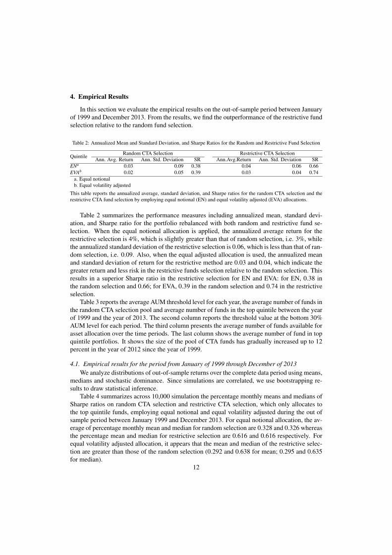
Table 2: Annualized Mean and Standard Deviation, and Sharpe Ratios for the Random and Restrictive Fund Selection
Quintile Random CTA Selection Restrictive CTA SelectionAnn. Avg. Return Ann. Std. Deviation SR Ann.Avg.Return Ann. Std. Deviation SR
This table reports the annualized average, standard deviation, and Sharpe ratios for the random CTA selection and therestrictive CTA fund selection by employing equal notional (EN) and equal volatility adjusted (EVA) allocations.
Table 2 summarizes the performance measures including annualized mean, standard devi-ation, and Sharpe ratio for the portfolio rebalanced with both random and restrictive fund se-lection. When the equal notional allocation is applied, the annualized average return for therestrictive selection is 4%, which is slightly greater than that of random selection, i.e. 3%, whilethe annualized standard deviation of the restrictive selection is 0.06, which is less than that of ran-dom selection, i.e. 0.09. Also, when the equal adjusted allocation is used, the annualized meanand standard deviation of return for the restrictive method are 0.03 and 0.04, which indicate thegreater return and less risk in the restrictive funds selection relative to the random selection. Thisresults in a superior Sharpe ratio in the restrictive selection for EN and EVA: for EN, 0.38 inthe random selection and 0.66; for EVA, 0.39 in the random selection and 0.74 in the restrictiveselection.
Table 3 reports the average AUM threshold level for each year, the average number of funds inthe random CTA selection pool and average number of funds in the top quintile between the yearof 1999 and the year of 2013. The second column reports the threshold value at the bottom 30%AUM level for each period. The third column presents the average number of funds available forasset allocation over the time periods. The last column shows the average number of fund in topquintile portfolios. It shows the size of the pool of CTA funds has gradually increased up to 12percent in the year of 2012 since the year of 1999.
4.1. Empirical results for the period from January of 1999 through December of 2013We analyze distributions of out-of-sample returns over the complete data period using means,
medians and stochastic dominance. Since simulations are correlated, we use bootstrapping re-sults to draw statistical inference.
Table 4 summarizes across 10,000 simulation the percentage monthly means and medians ofSharpe ratios on random CTA selection and restrictive CTA selection, which only allocates tothe top quintile funds, employing equal notional and equal volatility adjusted during the out ofsample period between January 1999 and December 2013. For equal notional allocation, the av-erage of percentage monthly mean and median for random selection are 0.328 and 0.326 whereasthe percentage mean and median for restrictive selection are 0.616 and 0.616 respectively. Forequal volatility adjusted allocation, it appears that the mean and median of the restrictive selec-tion are greater than those of the random selection (0.292 and 0.638 for mean; 0.295 and 0.635for median).
12
Table 3: The Threshold Level of AUM, the Average Number of Funds for Entire Universe and the Top Quintile Portfolio:Year 1999 through Year 2013
Year AUM Threshold Avg. Number of Funds Avg. Number of Funds in the Top Quintile1999 16,235,000 108 222000 13,008,333 109 222001 14,098,692 109 222002 11,773,625 117 232003 15,871,633 127 252004 20,156,742 136 272005 19,565,008 143 292006 21,254,775 146 292007 20,856,100 153 312008 25,088,608 166 332009 22,544,383 191 382010 23,794,733 204 412011 26,046,017 216 432012 24,939,333 230 462013 21,730,783 229 46
This table presents average threshold level of assets under management (AUM) at the bottom 30% level,number of funds available for allocation and number of funds in the top quintile for each year between 1999and 2013. The second column shows the average AUM threshold where is ranked on 70 percentile for eachperiod. The third column shows the average number of available CTA funds excluding bottom 30% AUMin each year. The last column reports the average number of funds that only including the upper 20% AUM.
Table 4: Annualized Mean and Standard Deviation, and Sharpe Ratios for the Random and Restrictive Fund Selection
Allocation Random CTA Selection Restrictive CTA Selection p-value (B1) p-value (B2)Mean Median Mean Median t-test signed t-test signed
This table reports the annualized average, standard deviation, and Sharpe ratios for the random CTA selection and therestrictive CTA fund selection by employing equal notional (EN) and equal volatility adjusted (EVA) allocations.
To examine the mean difference in monthly Sharpe ratios between the random selection andthe restrictive selection methods, we use the t-statistic, which tests the null hypothesis of meanequivalence. Also, to test the median difference in monthly Sharpe ratios between the randomselection and the restrictive selection methods, we conduct Wilcoxon singed rank test for the me-dian difference between the random selection and the restrictive selection in order to avoid outliereffect, which may mislead when comparing mean difference between samples. In addition, be-cause of our simulation results are not independent, we design two bootstrapping methods to carefor the robustness and the sensitivity of estimated mean and median from the empirical results.For the first bootstrapping method, all the p-values of the t-statistics for equal notional methodand equal volatility method reject the null hypothesis that no mean and median difference existsbetween the random selection and the restrictive selection at 5 % significant level. For the secondbootstrapping method, all p-values for equal notional allocation and equal volatility adjusted al-location are 0.00, which strongly indicates the null hypothesis of mean and median equivalencebetween the random selection and the restrictive selection should be rejected. In sum, it seems
1.9Wealth indices for equal volatility adjusted (EVA) allocation
Random CTA SelectionRestrictive CTA Selection
(b) Wealth indices for equal volatility ajusted al-location (EVA)
Figure 1: Cumulative Risk Adjusted Returns for the Random CTA Selection and the Restrictive CTA Selection betweenJanuary 1999 through December 2013
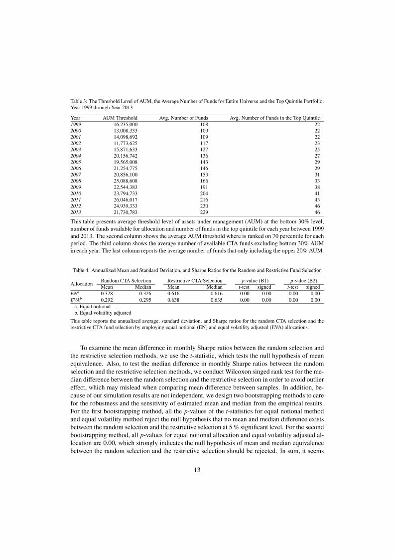
that restrictive CTA selection for both EN and EVA outperform the random CTA selection. 13
When we look through the performance of the restrictive CTA selection and the random CTAselection with respect to time, we see the outperformance persistence of the restrictive CTA se-lection against the random CTA selection as shown in Figure 1, which exhibits the cumulativerisk adjusted returns for the random CTA selection and the restrictive CTA selection for the pe-riod between January 1999 and December 2014. Panel A exhibits that in a case where the equalnotional allocation is applied, the solid line which represents the cumulative Sharpe ratio for therestrictive selection is mostly above the dotted line representing the cumulative risk adjusted re-turns along with the out-of-sample period. Panel B shows that in a case where the equal volatilityadjusted method is applied, the restrictive random selection that only includes the highest quintileportfolio ranked by asset under management outperforms relative to the random CTA selectionalong with the time horizon.
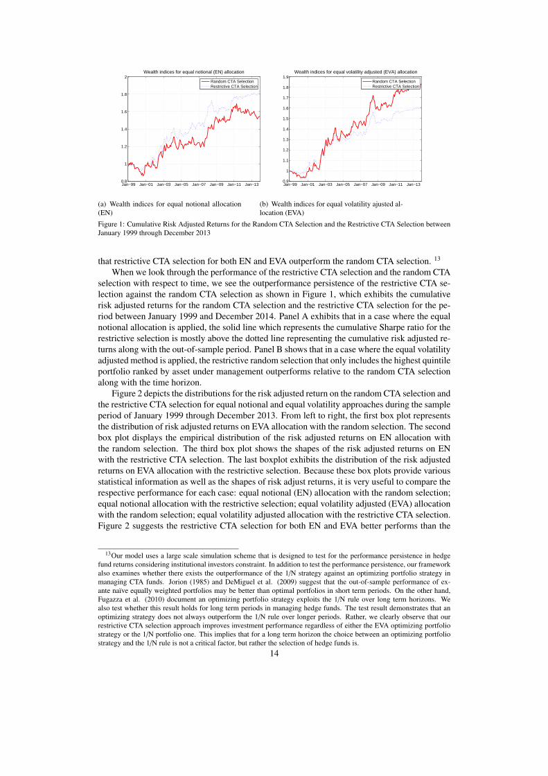
Figure 2 depicts the distributions for the risk adjusted return on the random CTA selection andthe restrictive CTA selection for equal notional and equal volatility approaches during the sampleperiod of January 1999 through December 2013. From left to right, the first box plot representsthe distribution of risk adjusted returns on EVA allocation with the random selection. The secondbox plot displays the empirical distribution of the risk adjusted returns on EN allocation withthe random selection. The third box plot shows the shapes of the risk adjusted returns on ENwith the restrictive CTA selection. The last boxplot exhibits the distribution of the risk adjustedreturns on EVA allocation with the restrictive selection. Because these box plots provide variousstatistical information as well as the shapes of risk adjust returns, it is very useful to compare therespective performance for each case: equal notional (EN) allocation with the random selection;equal notional allocation with the restrictive selection; equal volatility adjusted (EVA) allocationwith the random selection; equal volatility adjusted allocation with the restrictive CTA selection.Figure 2 suggests the restrictive CTA selection for both EN and EVA better performs than the
13Our model uses a large scale simulation scheme that is designed to test for the performance persistence in hedgefund returns considering institutional investors constraint. In addition to test the performance persistence, our frameworkalso examines whether there exists the outperformance of the 1/N strategy against an optimizing portfolio strategy inmanaging CTA funds. Jorion (1985) and DeMiguel et al. (2009) suggest that the out-of-sample performance of ex-ante naıve equally weighted portfolios may be better than optimal portfolios in short term periods. On the other hand,Fugazza et al. (2010) document an optimizing portfolio strategy exploits the 1/N rule over long term horizons. Wealso test whether this result holds for long term periods in managing hedge funds. The test result demonstrates that anoptimizing strategy does not always outperform the 1/N rule over longer periods. Rather, we clearly observe that ourrestrictive CTA selection approach improves investment performance regardless of either the EVA optimizing portfoliostrategy or the 1/N portfolio one. This implies that for a long term horizon the choice between an optimizing portfoliostrategy and the 1/N rule is not a critical factor, but rather the selection of hedge funds is.
14
Figure 2: The Distributions of the Sharpe Ratios for the Random Selection and the Restrictive Selection by EqualNotional Allocation and Equal Volatility Adjusted Allocation
random selection in a sense that the distributions for the restrictive method for EN and EVA rangebetween 0.37 and around 0.87 (0,37 through 0.84 for EN; 0.38 through 0.87 for EVA) whereasthe distributions for the random selection for EN and EVA are a range from -0.17 and 0.69 (0.09through 0.65 for EN; -0.17 through 0.69 for EVA).
To examine whether the performance of the restrictive CTA selection is better than the ran-dom CTA selection, we employ stochastic dominance, a comprehensive measure of portfolioreturn and variance. We also apply bootstrapping to treat sampling error in dominance testsas suggested by Post (2003) and Linton et al. (2010). Table 5 documents the first and secondstochastic dominance test for equal notional allocation and equal volatility adjusted allocation.Panel A shows the results of the first and second stochastic dominance tests on the basis of thefirst bootstrapping which considers less dependence across simulations. Kolmogrov-Smirnov(KS) statistics for EN and EVA provide evidence that the restrictive CTA selection has the firstand second stochastic dominance over the random CTA selection in the first bootstrapping casebecause all the p-values (for the first SD, 0.000 for EN and 0.000 for EVA; for the second SD,0.000 for EN and 0.000 for EVA) result in rejection of the null hypothesis that the restrictive se-lection does not stochastically dominate the random selection. Panel B reports the test results ofthe first and second stochastic dominance for the second bootstrapping approach which considerhigh level of dependence across simulations. All the p-values for Kolmogorov-Smirnov test (forthe first SD, 0.003 for EN and 0.003 for EVA; for the second SD, 0.003 for EN and 0.003 forEVA) reject the null hypothesis that no stochastic dominance exists between the random selectionand the restrictive selection for EN and EVA. Thus, Table 5 supports argument that the restrictedfund selection is superior to the random fund selection for all investors.
15
Table 5: First and Second Order Stochastic Dominance Tests
Allocation First Order SD Second Order SDKS p(KS ) KS p(KS )
This table reports results of the first and second stochastic dominance tests applied to distributions of Sharpe ratios de-rived using random and restrictive fund selection over the out-of-sample period between January of 1999 and Decemberof 2013. The first column displays the approach used to build portfolios. The second column reports the percentage oftime that the boostrapped distributions of Sharpe ratios have the first order stochastic dominance over the distributiongenerated using the random fund selection approach. The third column reports the p-value of the hypothesis that therestrictive fund selection does not dominate the Random fund selection using the bootstrapped approach. The fourth col-umn reports the percentage of time that the boostrapped distributions of Sharpe ratios have the second order stochasticdominance over the distribution generated using the random fund selection approach. The fifth column reports the p-value of the hypothesis that the restrictive fund selection does not dominate the random fund selection approach usingthe boostrapped distribution. The results are reported using the threshold level of AUM of 30%. Panel A reports resultsfor the first bootstrapped approach B1. Panel B present results for the second bootstrapped approach B2.
4.2. Fung and Hsieh Factor Analysis
Since higher Sharpe ratios can potentially be driven exposures to systematic sources of re-turns, we employ the Fung-Hsieh hedge funds risk factor models to test whether the restrictivefund selection results in a higher alpha (Fung and Hsieh, 2001, 2004). More specifically, we usethe Fung and Hsieh five factor model and seven factor model to examine it. Fundamentally, thosemodels are based on five trend following factors, two equity oriented risk factors, and two bondoriented risk factors. All the factors are from David A Hsiehs hedge fund data library 14 to es-tablish the Fung and Hsieh five factor model (Fung and Hsieh, 2001) and the seven factor model(Fung and Hsieh, 2004). The Fung and Hsieh five factor model of trend following systems in-cludes bond lookback straddle, currency lookback straddle, commodity lookback straddle, shortterm interest rate lookback straddle, and stock index lookback straddle. On the other hand, inorder to capture the systematic risk of a well diversified portfolio of hedge funds, the Fung andHsieh seven factor model consists of three trend following factors (bond trend following factor,commodity trend following risk factor, and currency trend following risk factor), two equity ori-ented market factors, and two bond oriented risk factors. The two equity oriented market riskfactors are i) the equity market factor, i.e. Standard & Poors 500 index monthly total return(Datastream item: S&COMP (RI)), and ii) the size spread factor, i.e. the spread between Russell2000 index monthly total return (Datastream item: FRUSS2L(RI)) and Standard & Poors 500monthly index total return (Datastream item: S&PCOMP(RI)) from DATASTREAM. The twobond oriented risk factors are i) a bond market factor, the monthly change in the 10 year constantmaturity yield from the Board of Governor of the Federal Reserve System 15, and ii) a credit
14David A. Hsiehs Data Library: https://faculty.fuqua.duke.edu/ dah7/HFRFData.htm15Constant maturity yields at the Board of Governors of the Federal Reserve System:
spread factor, defined as the monthly change in term spread between the Moodys Baa yield 16
and 10 year constant maturity yield.Additionally, to compare two alphas between the random selection and the restrictive selec-
tion, we test the significance of the difference between the alphas for the random selection andthe restrictive selection applying bootstrap experiment as suggested by Kosowski et al (2007)and Fung et al. (2008).
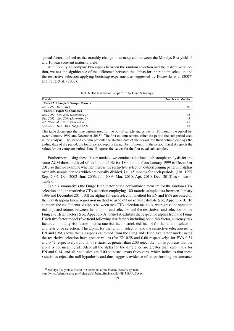
Table 6: The Number of Sample Size by Equal Subsample
Periods Number of MonthsPanel A. Complete Sample Periods
Jan. 1999 - Dec. 2013 180Panel B. Equal Sub-samples
This table documents the time periods used for the out-of-sample analysis with 180 month (the period be-tween January 1999 and December 2013). The first column reports either the period the sub-period usedin the analysis. The second column presents the starting date of the period, the third column displays theending date of the period, the fourth period reports the number of months in the period. Panel A reports thevalues for the complete period. Panel B reports the values for the four equal sub-samples.
Furthermore, using these factor models, we conduct additional sub-sample analysis for thesame AUM threshold level of the bottom 30% for 180 months from January 1999 to December2013 so that we examine whether there is the restrictive selection outperforming pattern in alphasover sub-sample periods which are equally divided, i.e., 45 months for each periods, (Jan. 1999Sep. 2002; Oct. 2002 Jun. 2006; Jul. 2006 Mar. 2010; Apr. 2010 Dec. 2013) as shown inTable 6.
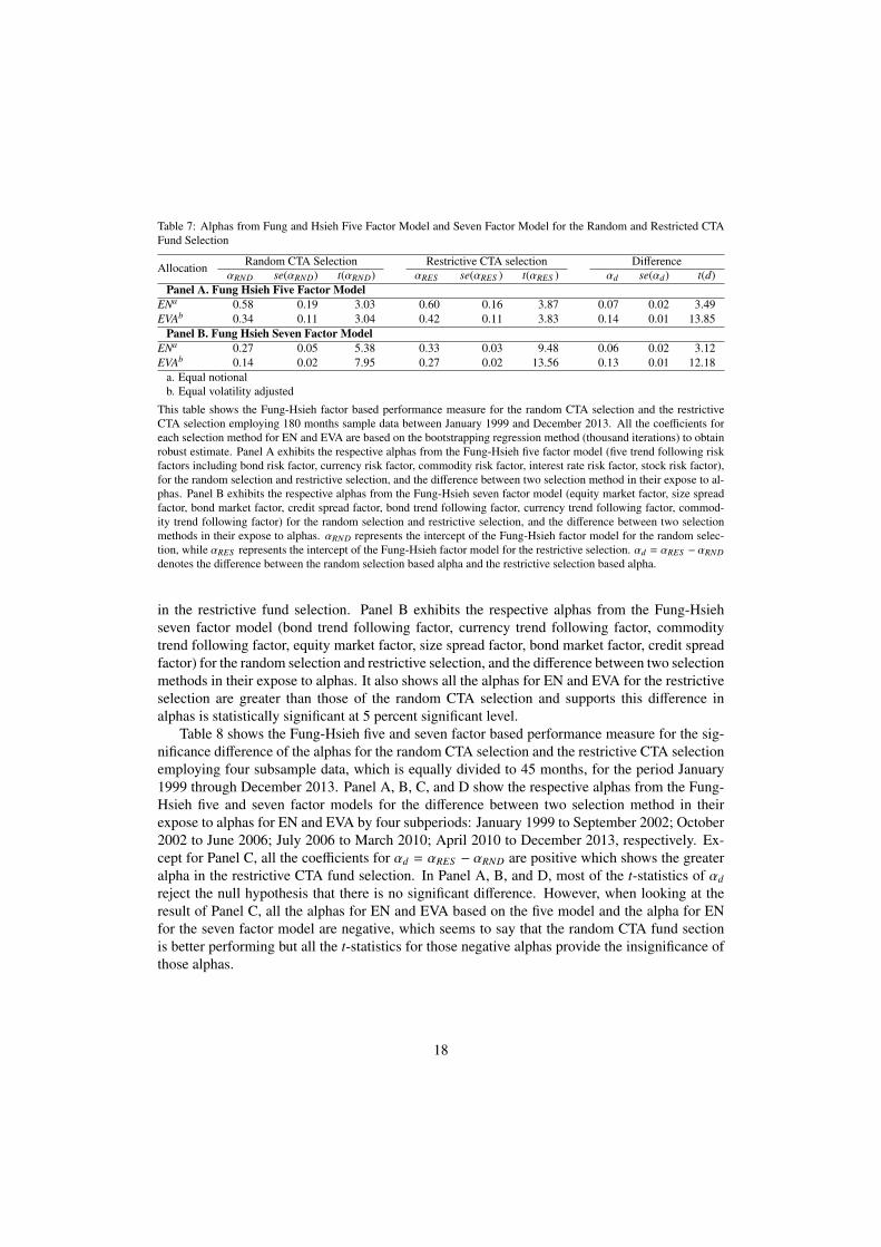
Table 7 summarizes the Fung-Hsieh factor based performance measure for the random CTAselection and the restrictive CTA selection employing 180 months sample data between January1999 and December 2014. All the alphas for each selection method for EN and EVA are based onthe bootstrapping linear regression method so as to obtain robust estimate (see, Appendix B). Tocompare the coefficients of alphas between two CTA selection methods, we regress the spread inrisk adjusted returns between the random fund selection and the restrictive fund selection on theFung and Hsieh factors (see, Appendix A). Panel A exhibits the respective alphas from the Fung-Hsieh five factor model (five trend following risk factors including bond risk factor, currency riskfactor, commodity risk factor, interest rate risk factor, stock risk factor) for the random selectionand restrictive selection. The alphas for the random selection and the restrictive selection usingEN and EVA shows that all alphas estimated from the Fung and Hsieh five factor model usingthe restrictive selection have greater values (for EN 0.58 and 0.60 respectively; for EVA 0.34and 0.42 respectively), and all of t-statistics greater than 2.00 reject the null hypothesis that thealpha is not meaningful. Also, all the alpha for the difference are greater than zero: 0.07 forEN and 0.14, and all t-statistics are 2.00 standard errors from zero, which indicates that theset-statistics reject the null hypothesis and thus suggests evidence of outperforming performance
16Moodys Baa yield at Board of Governors of the Federal Reserve system:http://www.federalreserve.gov/releases/h15/data/Business day/H15 BAA NA.txt
17
Table 7: Alphas from Fung and Hsieh Five Factor Model and Seven Factor Model for the Random and Restricted CTAFund Selection
This table shows the Fung-Hsieh factor based performance measure for the random CTA selection and the restrictiveCTA selection employing 180 months sample data between January 1999 and December 2013. All the coefficients foreach selection method for EN and EVA are based on the bootstrapping regression method (thousand iterations) to obtainrobust estimate. Panel A exhibits the respective alphas from the Fung-Hsieh five factor model (five trend following riskfactors including bond risk factor, currency risk factor, commodity risk factor, interest rate risk factor, stock risk factor),for the random selection and restrictive selection, and the difference between two selection method in their expose to al-phas. Panel B exhibits the respective alphas from the Fung-Hsieh seven factor model (equity market factor, size spreadfactor, bond market factor, credit spread factor, bond trend following factor, currency trend following factor, commod-ity trend following factor) for the random selection and restrictive selection, and the difference between two selectionmethods in their expose to alphas. αRND represents the intercept of the Fung-Hsieh factor model for the random selec-tion, while αRES represents the intercept of the Fung-Hsieh factor model for the restrictive selection. αd = αRES − αRNDdenotes the difference between the random selection based alpha and the restrictive selection based alpha.
in the restrictive fund selection. Panel B exhibits the respective alphas from the Fung-Hsiehseven factor model (bond trend following factor, currency trend following factor, commoditytrend following factor, equity market factor, size spread factor, bond market factor, credit spreadfactor) for the random selection and restrictive selection, and the difference between two selectionmethods in their expose to alphas. It also shows all the alphas for EN and EVA for the restrictiveselection are greater than those of the random CTA selection and supports this difference inalphas is statistically significant at 5 percent significant level.
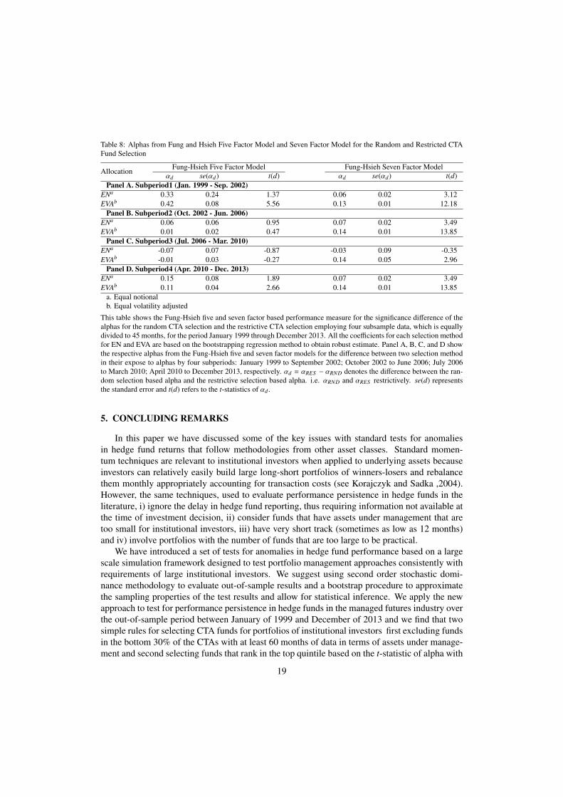
Table 8 shows the Fung-Hsieh five and seven factor based performance measure for the sig-nificance difference of the alphas for the random CTA selection and the restrictive CTA selectionemploying four subsample data, which is equally divided to 45 months, for the period January1999 through December 2013. Panel A, B, C, and D show the respective alphas from the Fung-Hsieh five and seven factor models for the difference between two selection method in theirexpose to alphas for EN and EVA by four subperiods: January 1999 to September 2002; October2002 to June 2006; July 2006 to March 2010; April 2010 to December 2013, respectively. Ex-cept for Panel C, all the coefficients for αd = αRES − αRND are positive which shows the greateralpha in the restrictive CTA fund selection. In Panel A, B, and D, most of the t-statistics of αd
reject the null hypothesis that there is no significant difference. However, when looking at theresult of Panel C, all the alphas for EN and EVA based on the five model and the alpha for ENfor the seven factor model are negative, which seems to say that the random CTA fund sectionis better performing but all the t-statistics for those negative alphas provide the insignificance ofthose alphas.
18
Table 8: Alphas from Fung and Hsieh Five Factor Model and Seven Factor Model for the Random and Restricted CTAFund Selection
Allocation Fung-Hsieh Five Factor Model Fung-Hsieh Seven Factor Modelαd se(αd) t(d) αd se(αd) t(d)
This table shows the Fung-Hsieh five and seven factor based performance measure for the significance difference of thealphas for the random CTA selection and the restrictive CTA selection employing four subsample data, which is equallydivided to 45 months, for the period January 1999 through December 2013. All the coefficients for each selection methodfor EN and EVA are based on the bootstrapping regression method to obtain robust estimate. Panel A, B, C, and D showthe respective alphas from the Fung-Hsieh five and seven factor models for the difference between two selection methodin their expose to alphas by four subperiods: January 1999 to September 2002; October 2002 to June 2006; July 2006to March 2010; April 2010 to December 2013, respectively. αd = αRES − αRND denotes the difference between the ran-dom selection based alpha and the restrictive selection based alpha. i.e. αRND and αRES restrictively. se(d) representsthe standard error and t(d) refers to the t-statistics of αd .
5. CONCLUDING REMARKS
In this paper we have discussed some of the key issues with standard tests for anomaliesin hedge fund returns that follow methodologies from other asset classes. Standard momen-tum techniques are relevant to institutional investors when applied to underlying assets becauseinvestors can relatively easily build large long-short portfolios of winners-losers and rebalancethem monthly appropriately accounting for transaction costs (see Korajczyk and Sadka ,2004).However, the same techniques, used to evaluate performance persistence in hedge funds in theliterature, i) ignore the delay in hedge fund reporting, thus requiring information not available atthe time of investment decision, ii) consider funds that have assets under management that aretoo small for institutional investors, iii) have very short track (sometimes as low as 12 months)and iv) involve portfolios with the number of funds that are too large to be practical.
We have introduced a set of tests for anomalies in hedge fund performance based on a largescale simulation framework designed to test portfolio management approaches consistently withrequirements of large institutional investors. We suggest using second order stochastic domi-nance methodology to evaluate out-of-sample results and a bootstrap procedure to approximatethe sampling properties of the test results and allow for statistical inference. We apply the newapproach to test for performance persistence in hedge funds in the managed futures industry overthe out-of-sample period between January of 1999 and December of 2013 and we find that twosimple rules for selecting CTA funds for portfolios of institutional investors first excluding fundsin the bottom 30% of the CTAs with at least 60 months of data in terms of assets under manage-ment and second selecting funds that rank in the top quintile based on the t-statistic of alpha with
19
respect to a CTA benchmark result in a significant improvement of performance. We evaluaterobustness of results across time period and find that our screening procedure consistently addsvalue with the exception of a relatively short data period. Our set of tests based on the simulationframework has practical importance for institutional investors because it helps discover easilyimplemented rules that can result in statistically significant improvements in investment perfor-mance as demonstrated in the case of momentum-based rules for hedge funds in the managedfutures industry.
Appendix A. Comparison of the Coefficients of the Alphas for the Random Fund Selectionand the Restrictive Fund Selection
Let αRES denote the alpha for the restrictive fund selection and let αRND denote the alphafor the random fund selection. Next, let d = αRES − αRND denote that the difference betweenthe restrictive selection based alpha and the random selection based alpha. In large sample case,under the assumption of equal variance we can test the significance of alphas between two fundselections as follows
Z = (αRES − αRND)/[s2(αRES ) + s2(αRND)]1/2 (A.1)
where s2(αRES ) represents the variance of the alpha for the restrictive selection, s2(αRND) repre-sents the variance of the alpha for the random selection, Z follows a standard normal distribution.However, this equal variance assumption is undesirable and practical for the comparison for thealpha estimates between two fund selections. Instead, we simply run bootstrapping linear regres-sion of the spread between the restrictive selection and the random selection in risk adjusted re-turn difference, i.e. the risk adjusted return for the restrictive fund selection less the risk adjustedreturn for the random fund selection, on the Fung and Hsieh factors. Let RRND = αRND + βRNDXbe the linear regression model for the random selection and RRES = αRES + βRES X be the linearregression model for the restrictive selection. Then the difference of two regression model iswritten as
where Rd = RRES − RRND, αd = αRES − αRND, and βd = βRES − βRND. Then from this we caneasily test the null hypothesis that
αd = αRES − αRND = 0 (A.4)
and use t-statisticst(αd) = αd/s(αd) (A.5)
for the test of the significance of alphas between two fund selections.
Appendix B. Alpha Estimations from the Bootstrapping Regression
The t-statistics of OLS may mislead if errors are non-normally distributed and violate i.i.dcondition. As Kosowski et al. (2007) and Fung et al. (2008) suggest this article estimate the
20
alphas of two group of funds based on the bootstrapping regression method to avoid type-I errorin estimating alphas and t-statistics of alphas to examine the validity of the alphas. We describethe bootstrapping procedure as follows.
Step 1. Regress the risk-adjusted return on the Fung-Hsieh risk factors for each fund i as
Ri,t = αi + βiXt + ϵi,t (B.1)
and estimate the residual asϵi,t = Ri,t − αi − βiXt (B.2)
Step 2. Draw T periods from t = 1, . . . ,T and produce a bootstrap sample by sampling ϵi,t.Denote Xb as a bootstrap sample where b is the number of bootstrapping. Denote theresample periods as t = sb
1, sb2, . . . , s
bT .
Step 3. Construct the resampled observations
Rbi,t = αi + βiXb
t + ϵi,t for t = sb1, s
b2, . . . , s
bT (B.3)
Step 4. Run the regression as
Rbi,t = α
bi + β
bi Xb
t + ϵi,t for t = sb1, s
b2, . . . , s
bT (B.4)
Step 5. Repeat step 2 for b = 1, . . . , B and compute t(αi) using the distribution of the standardbootstrap standard error of the alpha.
References
[1] Ackermann, C., McEnally, R., Ravenscraft, D., 1999. The performance of hedge funds: Risk, return, and incentives.Journal of Finance 54 (3), 833–874.
[2] Agarwal, V., Naik, N. Y., 2000a. Multiperiod performance persistence analysis of hedge funds. Journal of Financialand Quantitative Analysis 35 (3), 327–342.
[3] Agarwal, V., Naik, N. Y., 2000b. On taking the alternative route: The risks, rewards, and performance persistenceof hedge funds. Journal of Alternative Investments 2 (4), 6–23.
[4] Aragon, G. O., Nanda, V. K., 2014. Strategic delays and clustering in hedge fund reported returns. SSRN WorkingPaper available at http://papers.ssrn.com/sol3/papers.cfm?abstract id=2517611.
[5] Asness, C. S., Liew, J. M., Stevens, R. L., 1997. Parallels between the cross-sectional predictability of stock andcountry returns. Journal of Portfolio Management 23 (3), 79–87.
[6] Asness, C. S., Moskowitz, T. J., Pedersen, L. H., 2013. Value and momentum everywhere. Journal of Finance68 (3), 929–985.
[7] Beran, R., 1986. Discussion of wu, c.f.j.: Jackknife, bootstrap, and other resampling methods in regression analysis(with discussion). Annals of Statistics 14 (4), 1295 – 1298.
[8] Bhardwaj, G., G. B. Gorton, K. G. R., 2014. Fooling some of the people all of the time: The inefficient performanceand persistence of commodity trading advisors. Review of Financial Studies 27 (11), 3099 – 3132.
[9] Bhojraj, S., Swaminathan, B., 2006. Macromomentum: Returns predictability in international equity indices. Jour-nal of Business 79 (1), 429–451.
[10] Boudoukh, J., Richardson, M., Whitelaw, R. F., 1994. Industry returns and the Fisher effect. Journal of Finance49 (5), 1595–1615.
[11] Buraschi, A., Kosowski, R., Trojani, F., 2014. When there is no place to hide: Correlation risk and the cross-sectionof hedge fund returns. Review of Financial Studies 27 (2), 581 – 616.
[12] Cahart, M. M., 1997. On persistence in mutual fund performance. Journal of Finance 52 (1), 57–82.[13] Capocci, D., Hubner, G., 2004. Analysis of hedge fund performance. Journal of Empirical Finance 11 (1), 55–89.[14] Dardanoni, V., Forcina, A., 1999. Inference for Lorenz curve ordering. Econometrics Journal 2 (1), 49–75.
21
[15] DeMiquel, V., Garlappi, L., Uppal, R., 2009. Optimal versus naive diversification: How efficient is the 1/N portfoliostrategy? Review of Financial Studies 22 (5), 1915–1953.
[16] Diz, F., 1999. How do CTA’s return distribution characteristics affect their likelihood of survival? Journal ofAlternative Investments 2 (2), 37 – 41.
[17] Efron, B., 1979. Bootstrap methods: Another look at the jackknife. Annals of Statistics 7 (1), 1 – 26.[18] Efron, B., Gong, G., 1983. A leisurely look at the bootstrap, the jackknife, and cross validation. American Statisti-
cian 37 (1), 36 – 48.[19] Elton, E. J., Gruber, M. J., 1987. Modern portfolio theory and investment analysis. Wiley, New York.[20] Erb, C. B., Harvey, C. R., 2006. The strategic and tactical value of commodity futures. Financial Analysts Journal
62 (2), 69 – 97.[21] Fabozzi, F. J., Fuss, R., Kaiser, D. G., 2008. The Handbook of Commodity Investing. Wiley, Hoboken, New Jersey.[22] Fama, E. F., French, K. R., 1996. Multifactor explanations of asset pricing anomalies. Journal of Finance 51 (1),
55 – 84.[23] Fama, E. F., French, K. R., 2010. Luck versus skill in mutual fund returns. Journal of Finance 65 (5), 1915 – 1947.[24] Fischmar, D., Peters, C., 1991. Portfolio analysis of stocks, bonds, and managed futures using compromise stochas-
tic dominance. Journal of Futures Markets 11 (3), 259 – 270.[25] Flachaire, E., 2005. Bootstrapping heteroscedastic regression models: wild bootstrap vs. pairs bootstrap. Compu-
tational statistics and data analysis 49 (2), 361 – 379.[26] Fugazza, C., Guidolin, M., Nicodano, G., 2010. 1/n and long run optimal portfolios: Results for mixed asset menus.
Working Papers 2010-003, Federal Reserve Bank of St. Louis.[27] Fung, W., Hsieh, D. A., 2001. The risk in hedge fund strategies: Theory and evidence from trend followers. Review
of Financial Studies 14 (2), 313 – 341.[28] Fung, W., Hsieh, D. A., 2004. Hedge fund benchmarks: A risk based approach. Financial Analyst Journal 60 (5),
65 – 80.[29] Fung, W., Hsieh, D. A., Naik, N. Y., Ramadorai, T., 2008. Hedge funds: Performance, risk, and capital formation.
Journal of Finance 63 (4), 1777 – 1803.[30] Gorton, G. B., Hayashi, F., Rouwenhorst, K. G., 2013. The fundamentals of commodity futures returns. Review of
2003. Journal of Futures Markets 25 (8), 795 – 816.[32] Grinblatt, M., Moskowitz, T. J., 2004. Predicting stock price movements from past returns: The role of consistency
and tax-loss selling. Journal of Financial Economics 71 (3), 541 – 579.[33] Hadar, J., Russell, W., 1969. Rules for ordering uncertain prospects. American Economic Review 59 (1), 25 – 34.[34] Hanoch, G., Levy, H., 1969. The efficiency analysis of choices involving risk. Review of Economic Studies 36 (3),
335 – 346.[35] Hendricks, D., Patel, J., Zeckhauser, R., 1993. Hot hands in mutual funds: Short-run persistence of relative perfor-
mance, 1974-1988. Journal of Finance 48 (1), 93 – 130.[36] Jagannathan, R., Malakhov, A., Novikov, D., 2010. Do hot hands exist among hedge fund managers? An empirical
evaluation. Journal of Finance 65 (1), 217 – 255.[37] Jegadeesh, N., 1990. Evidence of predictable behavior of security returns. Journal of Finance 45 (3), 881 – 898.[38] Jegadeesh, N., Titman, S., 1993. Returns to buying winners and selling losers: Implications for stock market
efficiency. Journal of Finance 48 (1), 65 – 91.[39] Jenson, M., 1968. The performance of mutual funds in the period 1945-1964. Journal of Finance 23 (2), 389 – 416.[40] Joenvaara, J., Kosowski, R., Tolone, P., 2012. New stylized facts about hedge funds and database selection bias.
SSRN Working Paper available at http://papers.ssrn.com/sol3/ papers.cfm?abstract id=1989410.[41] Jorion, P., 1985. International portfolio diversification with estimation risk. Journal of Business 58 (3), 259 – 278.[42] Klecan, L., McFadden, R., McFadden, D., 1991. A robust test for stochastic dominance. Working Paper Department
of Economics, MIT.[43] Korajczyk, R. A., Sadka, R., 2004. Are momentum profits robust to trading costs? Journal of Finance 59 (3), 1039
– 1082.[44] Kosowski, R., Naik, N. Y., Teo, M., 2007. Do hedge funds deliver alpha? A Bayesian and bootstrap analysis.
Journal of Financial Economics 84 (1), 229 – 264.[45] Kroll, Y., Levy, H., 1980. Sampling errors and portfolio efficient analysis. Journal of Financial and Quantitative
Analysis 15 (3), 655 – 688.[46] Levy, H., Sarnat, M., 1970. Alternative efficiency criteria: An empirical analysis. Journal of Finance 25 (5), 1153
– 1158.[47] Linton, O., Song, K., Whang, Y., 2010. An improved bootstrap test of stochastic dominance. Journal of Economet-
rics 154 (2), 186 – 202.[48] Liu, R., 1988. Bootstrap procedure under some non-i.i.d. models. Annals of Statistics 16 (4), 1696 – 1708.
22
[49] Lo, A. W., MacKinaly, A. C., 1990. When are contrarian profits due to stock market overreaction? Review ofFinancial Studies 3 (2), 175 – 205.
[50] Malkiel, B. G., Saha, A., 2005. Hedge funds: Risk and return. Financial Analysts Journal 61 (6), 80 – 88.[51] Mammen, E., 1993. Bootstrap and wild bootstrap for high dimensional linear models. Annals of Statistics 21 (1),
255 – 285.[52] Molyboga, M., Baek, S., Bilson, J., 2014. CTA performance persistence: 1994 -2010. Journal of Alternative In-
vestments 16 (4), 61 – 70.[53] Moskowitz, T. J., Grinblatt, M., 1999. Do industries explain momentum? Journal of Finance 54 (4), 1249 – 1290.[54] Pastor, L., Stambaugh, R. F., 2002. Mutual fund performance and seemingly unrelated assets. Journal of Financial
Economics 63.[55] Porter, R. B., 1973. An empirical comparison of stochastic dominance and mean-variance portfolio choice criteria.
Journal of Financial and Quantitative Analysis 8 (4), 587 – 608.[56] Post, T., 2003. Empirical tests for stochastic dominance efficiency. Journal of Finance 58 (5), 1905 – 1931.[57] Rothschild, M., J, E. S., 1971. Increasing risk II: Its economic consequences. Journal of Economic Theory 3 (1),
66 – 84.[58] Rouwenhorst, K. G., 1998. International momentum strategies. Journal of Finance 53 (1), 267 – 284.[59] Schneeweis, T., Spurgin, R., 1996. Comparisons of commodity and managed futures benchmark indices. CISDM
Working Paper.[60] Schneeweis, T., Spurgin, R., Szado, E., 2013. Managed futures: A composite cta performance review. SSRN
Working Paper available at http://papers.ssrn.com/sol3/papers.cfm?abstract id=2205836.[61] Shleifer, A., Summers, L. H., 1990. The noise trader approach to finance. Journal of Economic Perspectives 4 (2),
19 – 33.[62] Wu, C., 1986. Jackknife boostrap and other resampling methods in regression analysis. Annals of Statistics 14 (4),