ABSTRACTTo draw valid inference about an indirect effect in a mediation model, there must be no omittedconfounders. No omitted confounders means that there are no common causes of hypothesizedcausal relationships. When the no-omitted-confounder assumption is violated, inference about indi-rect effects can be severely biased and the results potentiallymisleading. Despite the increasing atten-tion to address confounder bias in single-level mediation, this topic has received little attention inthe growing area of multilevel mediation analysis. A formidable challenge is that the no-omitted-confounder assumption is untestable. To address this challenge, we first analytically examined thebiasing effects of potential violations of this critical assumption in a two-level mediation model withrandom intercepts and slopes, in which all the variables are measured at Level 1. Our analytic resultsshow that omitting a Level 1 confounder can yield misleading results about key quantities of interest,such as Level 1 and Level 2 indirect effects. Second, we proposed a sensitivity analysis technique toassess the extent to which potential violation of the no-omitted-confounder assumptionmight inval-idate or alter the conclusions about the indirect effects observed. We illustrated the methods usingan empirical study and provided computer code so that researchers can implement the methods dis-cussed.
Mediation analysis has become popular in identifyingand testing causal mechanisms underlying psychologi-cal processes (Judd & Kenny, 1981; MacKinnon, 2008).For example, one can test whether the effect of studentacademic achievement (ACH; antecedent variable, X) onstudent career aspirations for the future (FUT; outcomevariable, Y) is mediated (completely or partially) by stu-dent academic self-concept (ASC;mediator,M). Figure 1adepicts linear relationships between the variables in thisexample, where a is the effect of X on M; b is the effectof M on Y controlling for X; c′ is the (direct) effect of Xon Y controlling for M; and c is the total effect of X on Yin Figure 1b. For this model, the indirect effect is equiva-lently represented as the product of coefficients, ab, or thedifference in coefficients, c − c′ (Pearl, 2012).
Because many questions in psychology that involvemediation processes are in the context of clustered data(e.g., clients nested within therapists, employees nestedwithin supervisors, observations nested within person),multilevel mediation is an extremely important tool thatis only recently becoming widely used because of theadvances in methodological explications and softwareto implement these complicated models (e.g., Lanaj,Johnson, & Barnes, 2014; Sturgeon, Zautra, & Arewasik-porn, 2014; Tofighi & Thoemmes, 2014; Wang et al.,
CONTACT Davood Tofighi [email protected] School of Psychology J. S. Coon Bldg., Georgia Institute of Technology, Cherry Street, Atlanta,Georgia –.Color versions of one or more of the figures in the article can be found online at www.tandfonline.com/hmbr.
Supplemental data for this article can be accessed at tandfonline.com/hmbr.
2013). As an example, consider the study by Nagengastand Marsh (2012), which examined the indirect effectof student ACH on student FUT through student ASC(self-perception of student academic skills). In this sce-nario, students (Level 1 units) are clustered (nested)within schools (Level 2 units). Because of the cluster-ing, student data within schools tend to be correlated.Because of the potential lack of independence amongstudent observations, traditional (single-level) techniquessuch as ordinary least squares (OLS) regression wouldproduce invalid inference about the coefficients (e.g.,underestimated standard errors; Raudenbush & Bryk,2002; Snijders & Bosker, 2012). Instead, researchersrecommend multilevel mediation analysis because it(a) correctly estimates the standard errors of the coeffi-cients, yielding more accurate inference of the indirecteffects (Kenny, Korchmaros, & Bolger, 2003; Krull &MacKinnon, 1999, 2001), (b) can estimate indirect effectsseparately at the student level (Level 1) and school level(Level 2; Preacher, 2011; Tofighi & Thoemmes, 2014), (c)can test whether the Level 2 indirect effect differs fromthe Level 1 indirect effect (Marsh, 1987; Marsh, Kuyper,Morin, Parker, & Seaton, 2014; Marsh, Trautwein,Lüdtke, Köller, & Baumert, 2005; Pituch & Stapleton,2012), and (d) can test whether a Level 2 variable mod-
Figure . A basic single-mediator model with an antecedent; X= academic achievement (ACH), a mediator; M = academic self-concept (ASC), and an outcome variable; Y = career aspirationsfor the future (FUT); εs denote residual terms. Rectangles showobserved variables. An arrow between two variables indicates adirect effect of the variable on the left on the other variable.
erates the Level 1 indirect effects (Bauer, Preacher, &Gil, 2006).
Despite the increasing popularity of multilevel medi-ation analysis, there remain key unresolved issues in thespecification and interpretation of important quantities.A salient issue that has received little attention is a dis-agreement about the proper way to estimate and inter-pret an indirect effect. Unlike the single-level media-tion model, the equality between ab or c − c′ does nothold inmultilevelmediation analysis under certain condi-tions (Tofighi, West, & MacKinnon, 2013). Some authorsargue that c − c′ is the proper estimate (Bauer et al.,2006; Kenny et al., 2003; Muthén & Muthén, 1998–2012;Preacher, 2011); other authors recommend ab as the cor-rect estimate (Tofighi&Thoemmes, 2014; Zhang, Zyphur,& Preacher, 2009).
We argue that such a discrepancy in defining an indi-rect effect is because of the lack of development in thearea of specification assumptions necessary to define andestimate a causal unbiased estimate of an indirect effectin a multilevel mediation model. Whereas the specifi-cation assumptions have garnered attention in single-level mediation analysis (e.g., Imai, Keele, & Tingley,2010; Judd & Kenny, 1981; Pearl, 2001; Valeri & Vander-Weele, 2013; VanderWeele, 2010), extending the speci-fication assumptions to the multilevel mediation mod-els has received little attention (Tofighi et al., 2013). Oneimportant part of the specification assumptions is the no-omitted-confounder assumption (Valeri & VanderWeele,2013; VanderWeele, 2010). The no-omitted-confounderassumption states that there must be no omitted commoncauses (i.e., confounders) of the observed variables in a
mediation model. The no-omitted-confounder assump-tion is critical to estimate an unbiased estimate of the indi-rect effect. Because the no-omitted-confounder assump-tion is untestable, the indirect effect is potentially biased(Holland, 1988). That is, we cannot rule out the biasingeffect of the potential confounders on the indirect effects.It is unfortunate that ramifications of potential violationof the no-omitted-confounder assumption have receivedlittle attention in the multilevel mediation literature.
In this article, we explicate the specification assump-tions necessary to define and estimate an unbiased causalindirect effect in a 1 → 1 → 1 multilevel mediationmodel. In the notation 1 → 1 → 1, the first, second, andthird number indicate that the antecedent, mediator, andoutcome variable, respectively, are measured at Level 1(Krull &MacKinnon, 2001).1 We show that a violation ofthe specification assumptions, especially the no-omitted-confounder assumption, is a source of major disagree-ment in defining and estimating an indirect effect. Thatis, when the no-omitted-confounder assumption is vio-lated, the two methods of defining and estimating indi-rect effect are no longer equal. In addition, estimates ofcoefficients would be biased, including the estimates ofindirect effects, because the indirect effects are functionsof the estimates of coefficients. Because the no-omitted-confounder assumption is untestable, we propose a sen-sitivity analysis technique to assess the extent to whichany potential violation of the no-omitted-confounderassumption would change the conclusions about the indi-rect effects.
Unresolved issues in multilevel mediationanalysis
The implications of violating the specification assump-tions, including the no-omitted-confounder assumption,have received little attention inmultilevel mediation anal-ysis. An exception is the work by Tofighi et al. (2013),which examined the biasing effects of omitting a Level 2(school-level), not a Level 1 (student-level), confounderin a 1 → 1 → 1 model. Tofighi et al. assumed that theomitted Level 2 confounder was correlated with themedi-ator and outcome variable, not the antecedent variable.They found that the omitted Level 2 confounder wouldbias the estimates of the indirect effect at Level 1 and biasthe variance–covariance estimates at Level 2. Tofighi et al.concluded that the interpretation of indirect effects wouldbecome ambiguous in the presence of the omitted con-founder.
We will also discuss additional types of multilevel mediation models such as→ → model, in which X is measured at Level .
Dow
nloa
ded
by [U
nive
rsity
of N
otre
Dam
e] a
t 05:
06 1
8 Fe
brua
ry 2
016
88 D. TOFIGHI AND K. KELLEY
Several important issues remain unresolved. First,Tofighi et al. (2013) considered the biasing effects of aLevel 2 (e.g., school-level), not a Level 1 (e.g., student-level) omitted confounder. Second, Tofighi et al. studieda simplified case in which the Level 2 omitted confounderwas assumed to influence themediator and outcome vari-able but not the antecedent variable. Cases in which theomitted confounder influences all of the observed vari-ables at both levels of analysis were not considered. There-fore, Tofighi et al.’s results are limited to randomizedexperimental studies in which omitted confounders onlyexist at Level 2.
We discuss three scenarios in which omitted con-founders can arise in practice (Lash, Fox, & Fink, 2009):
1. Observational or experimental mediation studieswith a single unmeasured, but known, confounderat Level 1. This scenario might occur when a the-ory exists about the relevant Level 1 confounderand yet the confounder is unmeasured. This islikely to happen in archival data sets, in whicha researcher might not have had control of thechoice of variables being measured.
2. Observational or experimental mediation stud-ies with an unknown confounder or confounders.This scenario occurs when a researcher does nothave a theory about the nature of omitted vari-ables. For example, theoretical development andsubstantive theory have not progressed enough toidentify all of the possible omitted confounders.
3. Observational or experimental mediation stud-ies with multiple unmeasured confounders, wherea theory identifies important unmeasured con-founders and their relationships with the observedvariables. These confounders are neithermeasurednor included in the study (e.g., an archival dataset).
In this article we present a framework that can examinethe biasing effect of omitted confounder(s) in Scenarios 1and 2. We do not address Scenario 3 because it is beyondthe scope of this article.
Another unresolved issue is how to assess the extentto which indirect effect estimates might be biased. Forthis, we develop a method to assess sensitivity of indi-rect effect estimates to the potential violations of theno-omitted-confounder assumption. Because the no-omitted-confounder assumption is not testable (Hol-land, 1988), epidemiologists have recommended thatresearchers probe the sensitivity of indirect effects topotential violation of the no-unmeasured-confounderassumption (Blakely, 2002; Hafeman, 2011). Sensitivityanalysis helps researchers determine how sensitive theestimates of indirect effects are to the potential violationsof the no-omitted-confounder assumption.
Goals
We first study the multilevel biasing effects of an omit-ted Level 1 confounder on the interpretation and estima-tion of indirect effects at both Level 1 and Level 2 fora two-level 1 → 1 → 1 mediation model with randomintercepts and slopes. A key goal is to assess the biasingeffects of an omitted Level 1 confounder that is correlatedat both Levels 1 and 2 with all the variables in a multi-levelmodel.We extend the single-levelmediation analysisframework (Cox, Kisbu-Sakarya, Miocevic, & MacKin-non, 2013) to analytically examine the multilevel biasingeffects by decomposing Level 1 confounder(s) into twoorthogonal components. We analytically derive expres-sions quantifying the magnitudes of confounder bias onthe Level 1 and Level 2 coefficients and indirect effects aswell as the Level 2 variance of the random indirect effect.
The second goal is to assess the extent to which multi-level omitted confounder bias would change conclusionsabout Level 1 and Level 2 indirect effects, which we dousing a sensitivity analysis. The sensitivity analysis offersestimates of the amount of bias in key estimates that helpbracket the likelymagnitude of the true indirect effect hadit been modeled with the confounders included. The sen-sitivity analysis addresses the following questions:
1. How large is the relationship between the omittedconfounders andX,M, andY that would yield zero(or nonsignificant) estimates of indirect effects atLevel 1 or 2?
2. What are the estimates of indirecteffects when omitted confounders are(not/moderately/strongly) correlated with X,M, and Y?
We will show how the sensitivity analysis can answerthese important research questions in the context of theaforementioned empirical example.
In the single-level single-mediator model, there areseveral techniques to address the potential violation of theno-omitted-confounder assumption (see MacKinnon &Pirlott, 2015; for a detailed discussion, see Cox et al.,2013). We extend the sensitivity analysis method devel-oped for the single-level single-mediator model (Coxet al., 2013) to the 1 → 1 → 1 model to assess potentialbias for the two types of the omitted confounder(s) dis-cussed in Scenarios 1 and 2. Cox et al.’s sensitivity analy-sis is an extension of Mauro’s (1990) technique that usedthe correlation of an omitted variable with the observedvariables in OLS regression to assess changes in the con-clusions about regression coefficients. The advantage ofour method is that it extends the technique based on thecorrelations of omitted confounder(s) with the observedvariables to both observational and experimental studies(less X) in multilevel mediation studies.
Dow
nloa
ded
by [U
nive
rsity
of N
otre
Dam
e] a
t 05:
06 1
8 Fe
brua
ry 2
016
MULTIVARIATE BEHAVIORAL RESEARCH 89
Background: Multilevel mediationmodel
Before proceeding further, we present background andnecessary equations to specify a two-level, 1 → 1 → 1model with random intercepts and slopes. The resultspresented in our study are general, but for concretenesswe use the aforementioned education example through-out the manuscript. Consider again the empirical exam-ple by Nagengast and Marsh (2012). In this 1 → 1 →1 model, the random slopes capture the heterogeneity ofLevel 1 (Within) effects across schools; the random inter-cepts model the Level 2 (Between) relationships. Othertwo-levelmediationmodels such as 2→ 1→ 1 and 2→ 2→ 1have also beenproposed (Krull&MacKinnon, 2001).We focus on the 1→ 1→ 1modelwith random interceptsand slopes because it is the most detailed and complexmodel. It has the greatest number of both fixed (at least sixcoefficients, three for each level of analysis) and randomeffects (ten Level 2 covariances, five Level 2 variances,and two Level 1 variances) compared to other similarmodels.
For our educational example, we derive analyticalresults using centering within cluster 2 (CWC2) withlatent cluster means for the following reasons, some ofwhich are outlined by Marsh et al. (2009); CWC2 cen-ters variables within cluster (school) and adds the clus-ter (school) means as covariates into the model at Level 2.First, our research question guided the choice of cen-tering strategy (Enders & Tofighi, 2007). In our exam-ple, we are interested in whether a student ASC is apositive function of student ACH and a negative func-tion of school-average ACH score. Students with higherACH scores are expected to have higher ASC. However,academically selective schools with high-ability studentsmight negatively influence student ASC. Such a differ-ential effect in the school-level (Between) and student-level (Within) ACH→ASC is a contextual effect knownas the big-fish-little-pond effect (BFLPE; Marsh, 1987).In addition, we chose CWC2 to clearly show the effectof an omitted confounder bias on Between, Within, andcross-level effects in the model. Using CWC2 simplifiedthe analytical results because it allowed us to decom-pose Between and Within effects for the observed vari-ables as well as the confounder(s). We chose using latentcluster means instead of observed cluster means to beconsistent with results in Marsh et al. (2009). Marshet al. recommended using latent mean centering for thisproblem. In addition, using latent cluster means is likelyto produce less attenuated estimate of Between effects(Lüdtke et al., 2008).2
We provide a more extensive treatment of centering of the predictors in→ → models in the supplemental materials.
Equations for the 1→ 1→ 1model
The first set of equations decompose Xij,Mij, and Yij intothe orthogonal Level 2 and Level 1 latent variables usingCWC2 with latent cluster means, where i denotes a stu-dent and j denotes a school:
In Equation (1), ηXj is the Level 2 latent school (cluster)mean on ACH; this is a random intercept that is schoolspecific. The within-school (Within) latent component,ηXij, measures the deviation of each student’s ACH scorefrom his or her school’s latent mean. This score showsthe standing of each student relative to his or her school’slevel. For the mediator and outcome variables in (2) and(3), respectively, the Between components, ηMj and ηYj,represent latent school means on ASC and FUT, respec-tively. For Mij and Yij, the Within components ηMij andηYij represent student i’s deviation score from his or herschool’s latent mean, respectively. For example, ηMij rep-resents the standing of a particular student’s ASC relativeto his or her latent school mean on ASC.
A common practice in specifying a multilevel media-tion model is to write equations for Level 1 (e.g., student)and Level 2 (e.g., school). Separately, the Level 1 equationsfor the population relationships at the student level are
Mij = ηMj + a jηXi j + εMi j (4)Yi j = ηY j + c′jηXi j + b jηMi j + εYi j. (5)
The Level 2 equations for the relationships at the schoollevel are
ηMj = d0M + aBηX j + uMj (6)ηY j = d0Y + c′BηX j + bBηMj + uY j (7)a j = aW + ua j (8)b j = bW + ubj (9)c′j = c′W + uc′ j. (10)
One can also specify the following Level 1 and 2 equa-tions to estimate the population total effect of ACH onFUT:
Yi j = ηY j + c jηXi j + ε′Yi j (11)
ηY j = d′0Y + cBηX j + u′
Y j (12)c j = cW + uc j. (13)
Equations (4), (5), and (11) describe population rela-tionships between observed variables for each Level 1 uniti (e.g., student). For example, Equation (4) shows that stu-dent ACH predicts ASC. Coefficient aj is the latent effect
Dow
nloa
ded
by [U
nive
rsity
of N
otre
Dam
e] a
t 05:
06 1
8 Fe
brua
ry 2
016
90 D. TOFIGHI AND K. KELLEY
of ACH on ASC for Level 2 unit j (e.g., school). The sub-script j indicates that this effect can vary across schools.Because aj is unobserved and varies across schools, it isalso called a random effect (coefficient); bj is the randomeffect of ASC on FUT, while controlling for ACH; c′j is therandom effect of ACH on FUT, while controlling for ASC;cj is the total random effect of ACHonFUT. The εs denotethe Level 1 residuals.
Because we used CWC2, Level 2 Equations (6), (7),and (12) describe the Level 2 (Between) population coef-ficients. The Between coefficients are denoted by the sub-script “B”: aB is the Between effect of ACH on ASC; bB isthe Between effect of ASC on FUT, while controlling forACH; c′B is the Between effect of ACH on FUT, while con-trolling for ASC; and cB is the Between total effect of ACHon FUT.
Finally, the Level 2 Equations (8)–(10) and (13)describe the relationships between random coefficientsand population-average coefficients (i.e., the expected val-ues of the random coefficients) for each Level 2 unit j. Thepopulation-average coefficients are the Level 1 (Within)coefficients denoted by the subscript “W”. For example,Equation (8) shows that aj equals the population-averageWithin coefficient, aW, which is the expected value ofall ajs across all the schools, plus a deviation from thepopulation-average coefficient for school j, denoted byuaj.Henceforth, we call the population-averageWithin coeffi-cients simplyWithin coefficients. TheWithin coefficients,bW, c′W , and cW, have similar interpretation as the popula-tion average for their respective random coefficients. Theu terms, which denote deviations from the Within coeffi-cients, are also referred to as Level 2 residuals.
Distributional assumptions
In a 1 → 1 → 1 model, distributional assumptions aboutthe residuals are critical in obtaining unbiased estimatesof indirect effects (Bauer et al., 2006; Tofighi et al., 2013).Here, we provide a general description of the distribu-tional assumptions.
The vector of Level 1 (Within) residuals is denoted byε = (εMi j, εYi j)
T, where T denotes vector transpose. Thevector of residuals is assumed to have a bivariate normaldistribution with the means of zero and a 2×2Within thevariance–covariance matrix denoted by !W :
!W =(
σ 2εMi j
σεMi j,εYi j σ 2εYi j
)
, (14)
where the terms σ 2εMi j
and σ 2εYi j
are variances and σεMi j,εYi j
is the covariance between Level 1 residuals across theequations associated withM and Y.
The vector of Level 2 residual terms, u =(uMj, uaj , uYj , ubj , uc′j )
T , contains five residual termsassociated with M and Y in Equations (6)–(10), twofor the random intercepts and three for random slopes.The vector is assumed to have a multivariate normaldistribution with the means of zero and a 5×5 Betweenvariance–covariance matrix, !B, as follows:
!B =
⎛
⎜⎜⎜⎜⎜⎜⎝
σ 2uMj
σua j ,uMj σ 2ua j
σuYj ,uMj σuYj ,ua j σ 2uYj
σub j ,uMj σub j ,ua j σub j ,uYj σ 2ub j
σuc′j ,uMj σuc′j ,ua jσuc′j ,uYj
σuc′j ,ub jσ 2uc′j
⎞
⎟⎟⎟⎟⎟⎟⎠(15)
The off-diagonal elements are the covariances betweenpairs of the residual terms (or, equivalently, randomeffects). Considering !B, we delineate subtle, but impor-tant, differences between two types of covariancesbetween residuals in a 1 → 1 → 1 model (Bauer et al.,2006). The 1 → 1 → 1 model is a bivariate model thatconsists of two Level 1 equations with two dependentvariables (i.e., M and Y). The covariances in the 1 → 1→ 1 model contain both within-equation and between-equation covariances. Interpretation of within-equationcovariances in a 1 → 1 → 1 model is similar to that in aconventional univariate multilevel model (Raudenbush &Bryk, 2002). For example, uaj and uMj both appear in theLevel 2 equations for the mediator M. When an appro-priate centering strategy is applied, Snijders and Bosker(2012, Chapter 5) recommend estimating and interpret-ing thewithin-equation covariances. For example, within-equation covariance σua j ,uMj is the covariance between therandom intercept and slope predicting the same depen-dent variable, M. A negative value for this covariancecould indicate that the higher the school-average ACH,the smaller the relationship between student ACH andASC. Between-equation covariances, however, are spe-cific to amultivariatemodel such as the 1→ 1→ 1model.In a conventional multilevel model, there are no between-equation covariances. Unlike within-equation covariance,a nonzero between-equation covariance might not have asubstantive interpretation (Tofighi et al., 2013).
Level 1 and Level 2 indirect effects
In multilevel analysis, indirect effects can be defined ateach level. First, we discuss the random indirect effectthat is the product of two random coefficients: ajbj. UsingCWC2, we define the random indirect effect as a school-specific, Within indirect effect for school j that variesrandomly around the population-averageWithin indirecteffect, aWbW, or, simply, Within indirect effect.
Dow
nloa
ded
by [U
nive
rsity
of N
otre
Dam
e] a
t 05:
06 1
8 Fe
brua
ry 2
016
MULTIVARIATE BEHAVIORAL RESEARCH 91
A point of contention is whether the expected valueof the random indirect effect equals the (Within) indirecteffect. Several authors broadly define indirect effect as theexpected value of the random indirect effect (Bauer et al.,2006; Kenny et al., 2003; Preacher, 2015; Preacher, Zyphur,& Zhang, 2010). When CWC2 is applied, these authorsdefine the Within indirect effect as follows:
E[a jb j] = aWbW + σa j,b j , (16)
where σa j,b j is the covariance between the randomeffects aj and bj, or equivalently, between the respectiveLevel 2 residuals (Tofighi et al., 2013). However, Tofighiet al. showed that when there is an omitted confounderat Level 2, the expression does not estimate an unbiasedestimate of the Within indirect effect. Next, we provide aset of specification assumptions necessary to compute anunbiased estimate of an indirect effect.
Specification assumptions
We extend the specification assumptions from the single-level mediation literature in different methodological tra-ditions (e.g., path analysis and counter-factual frame-work) to the multilevel mediation analysis (James, 1980;James & Brett, 1984; Judd & Kenny, 1981; McDonald,1997; Pearl, 2001; Valeri & VanderWeele, 2013; Van-derWeele, 2010). Investigating the correct specificationassumptions inmediation analysis ismore challenging fora 1 → 1 → 1 model than for a single-level model. Thechallenges result from the complex nature of the multi-level data. For example, in a 1 → 1 → 1 model (a) therelationships might exist at two levels of analysis; (b) theinteraction effects might occur at either level or across thelevels; or (c) each variablemight bemeasured at Level 1 or2, resulting inmodels with distinct interpretations of indi-rect effects (e.g., e.g., 2→ 1→ 1 model; Krull &MacKin-non, 1999, 2001; Pituch & Stapleton, 2012). As discussed,scaling predictors plays an important role in estimationand interpretation of the model parameters (Enders &Tofighi, 2007; Lüdtke et al., 2008; Preacher, 2011; Zhanget al., 2009). Finally, distributional assumptions about theresiduals are more complicated in a multilevel model. Forthe 1 → 1 → 1 model, as shown previously, one needsto make distributional assumptions about seven residualsinstead of two residuals in the single-mediator model inFigure 1.
A correctly specifiedmodel
For a correctly specified 1 → 1 → 1 model, the followingset of specification assumptions is necessary to have anunbiased estimate of indirect effects:
1. Correct functional forms: The functional relation-ships as well as the causal order of the relationshipsbetween X,M, and Y are correctly specified.
2. Validity and reliability: The observed variables X,M, and Y are perfectly valid and perfectly reliablemeasures of the respective constructs.
3. No method bias: Method bias might occur whentwo or more variables in a study are measuredusing the same method of measurement (Camp-bell & Fiske, 1959; Podsakoff, MacKenzie, Lee, &Podsakoff, 2003; Richardson, Simmering, & Stur-man, 2009). For example, if the observed vari-ables in a mediation study are collected using aself-report questionnaire, a researcher might sus-pect that “at least some of the observed covaria-tion between themmay be due to the fact that theyshare the same method of measurement” (Pod-sakoff, MacKenzie, & Podsakoff, 2012, p. 540). Theno method bias assumption states that there existsno shared method variance biasing the relation-ships between X,M, and Y at either level.
4. No omitted confounder: There is no omitted con-founder of the X, M, and Y relationships at eitherlevel of analysis. More formally, this assump-tion states that there must be no omitted con-founders of the relationships between X, M, andY that are posited in the 1 → 1 → 1 model inEquations (1)–(10). The no-omitted-confounderassumption has also been termed the “no omit-ted variables” assumption (MacKinnon & Pir-lott, 2015), “orthogonality of residuals” assump-tion (McDonald, 1997), and “sequential ignorabil-ity” assumption (Imai et al., 2010).
5. No interaction: No interaction effect existsbetween the observed variables as well as betweenthe observed and omitted variables at each leveland across levels. This assumption is also referredto as the “no-interaction,” “linearity,” or “constant-effect” assumption (Pearl, 2012).
Finally, as we discussed previously, the distributionalassumptions aboutmultilevelmodelsmust also bemet forproper statistical inference (e.g., confidence interval [CI]and p values; Raudenbush & Bryk, 2002).
Assumption 1 emphasizes the longitudinal nature ofa mediation model in that X is measured before M andM is measured before Y (Davis, 1985; MacKinnon, 2008).Cross-sectionalmediation studies in which this conditionis not met can lead to invalid results (Maxwell & Cole,2007; Maxwell, Cole, & Mitchell, 2011). When the aboveassumptions hold, Tofighi et al. (2013) showed that
aBbB = cB − c′B (17)aWbW = cW − c′W . (18)
Dow
nloa
ded
by [U
nive
rsity
of N
otre
Dam
e] a
t 05:
06 1
8 Fe
brua
ry 2
016
92 D. TOFIGHI AND K. KELLEY
This result indicates that both methods of calculat-ing Level 1 and Level 2 indirect effects are equivalent.It also implies that both the product-of-coefficient anddifference-in-coefficients methods will produce an unbi-ased estimate of indirect effects at the respective levelsof analysis. Assumptions 2, 3, and 5, which are not dis-cussed by Tofighi et al. (2013), are also critical in obtain-ing equivalent unbiased estimates of the indirect effectsusing either method. When these assumptions hold, anunbiased, causal estimate of the Within indirect effectis E[a jb j] = aWbW = cW − c′W . In addition, covariancebetween aj and bj will be zero: σa j,b j = 0. That is, whenthese assumptions hold, we can define and estimate acausal estimate of the Within indirect effect. However, aswill be shown later, if Assumptions 3 and 5 are violated,the relationships in Equations (17) and (18) do not hold.More important, Equation (16) does not provide a causal,unbiased estimate of Within indirect effect.
Amisspecifiedmodel
To investigate the implications of violation of the no-omitted-confounder assumption, we consider a “misspec-ified” 1 → 1 → 1 model in which the omitted con-founder(s) of X, M and Y relationships may exist at bothlevels. We consider the types of omitted confounder(s)in Scenarios 1 and 2: single unmeasured confounder andunknown confounder(s). In terms of the specificationassumptions, we assume that Assumptions 4 and 5 areviolated, whereas Assumptions 1–3 hold. For this mis-specifiedmodel, estimating biasing effects of omitted con-founder(s) poses the following challenges.
Challenge One key challenge that arises when a potential con-founder is correlated with the observed variables atboth levels of analysis is that the resulting compounded,multilevel biasing effects can be comprised of Level 1,Level 2, and cross–level effects. That is, a confounder maynot only bias the relationships at Level 1 and Level 2, butmay also serve as a potential moderator of the Level 1relationships. This result implies that the no-interactionassumption can also be violated. This violation occursbecause the Level 1 omitted variable that varies at bothLevels 1 and 2 can also moderate the Within coefficientsthat substantially vary across Level 2 units (e.g., acrossschools). In this case, the Within indirect effect would bemoderated by omitted confounders at Level 2 (e.g., schoolcharacteristics). Thus, we can have an omitted cross-levelinteraction effect. In addition, omitted confounders atthe individual level (e.g., student characteristics) can alsomoderate the Level 1 indirect effect. In this case, we canhave an omitted Level 1 interaction effect.
We investigate the important case of the omitted con-founder effect on cross-level interaction.3 A cross-leveleffect is of substantive importance in various areas ofpsychological research and related fields (Raudenbush& Bryk, 2002; Snijders & Bosker, 2012). Omitted cross-level interaction effects are of substantive interest inschool settings; for example, educational researchers areoften interested in estimating environmental factors (e.g.,school-district characteristics) affecting student perfor-mance and what school-level characteristics would mod-erate student-level indirect effects.
Challenge A second challenge is finding a mathematical frameworkthat computes and estimates the biasing effects of omit-ted confounder(s). Themathematical framework needs toconsider that potential biasing effects of an omitted con-founder are likely to be a weighted composite of unob-served Level 1 and Level 2 correlations (Kreft, de Leeuw,&Aiken, 1995). To estimate the weighted composite effectof the omitted variable, values for three unobserved quan-tities are needed: (a) Level 2 correlations of an omittedconfounder with the observed variables, (b) Level 1 corre-lations of an omitted confounder with the observed vari-ables, and (c) the weights for the composite effect.
Method
Assessing omitted confounder bias
Mauro (1990) described techniques to assess the poten-tial biasing effect of an omitted variable in OLS regres-sion. Cox et al. (2013) extended these techniques to assessomitted confounder bias in a single-level single-mediatormodel. We extend this framework for 1→ 1→ 1 models.We describe three critical stages in the extended frame-work: First, we introduce the concept of a latent proxyvariable to model confounder bias in Scenarios 1 and 2.Second, we discuss the concept of “augmented” model.Third, we describe the necessity of reexpressing relation-ships between the latent proxy variable and observed vari-ables to derive analytic results.
Latent proxy variableTo address Challenge 1, we introduce a single latent vari-able, Zij, that serves as a proxy for omitted confounder(s)that may exist at both Levels 1 and 2. First, we assumethat the latent proxy variable, Zij, is potentially corre-lated with all of the observed variables (i.e., the no-omitted-confounder assumption is violated); the sign and
Deriving analytic results for both omitted cross-level and Level interactioneffects is beyond the scope of this manuscript.
Dow
nloa
ded
by [U
nive
rsity
of N
otre
Dam
e] a
t 05:
06 1
8 Fe
brua
ry 2
016
MULTIVARIATE BEHAVIORAL RESEARCH 93
the magnitude of the correlations may vary. Second, weassume that the latent proxy variable linearly influencesthe observed variables in the model. That means thatpotential nonlinear relationship (e.g., quadratic relation-ship) between the omitted and observed variables are notmodeled.
The use of Zij as a proxy for the potential omittedconfounder(s) is justified because a single latent variableis sufficient to account for spurious correlations (covari-ances) between (residuals of) three observed variables(Brewer, Campbell, & Crano, 1970). By spurious we meanextraneous correlation not accounted for by the positedmediation model. When the no-omitted-confounderassumption is violated, between-equation covariances in$W in (14) and $B in (15) will be nonzero;4 otherwise,the between-equation covariances will be zero if speci-fication assumptions 1–5 hold. Introducing Zij accountsfor the spurious correlations between observed vari-ables, thereby rendering the between-equation covari-ances zero. In addition, because the potential omitted con-founders are likely to explain heterogeneity of indirecteffects across Level 2 units, we investigate whether Zijmoderates the Level 1 indirect effect, violating the no-interaction assumption. It should be noted that Zij servesas a proxy for both Level 1 and Level 2 confounders.
The latent proxy variable is suitable to addressconfounder-bias in Scenarios 1 and 2. In Scenario 1, fora single known unmeasured confounder, a researcher ismore likely to find plausible values for the correlations ofthe unmeasured confounder with the observed variablesfrom the literature or experts. A researcher can use thislatent proxy variable along with the range of the correla-tion values to evaluate the potential biasing effect on theconclusions about the indirect effect.
For the unknown confounders in Scenario 2, the latentproxy variable assumes that the effect of all unknown con-founders can be represented by a single latent variable.Making this assumption is reasonable because researchershave made similar types of assumptions about unknowncauses when specifying disturbances in single-level struc-tural equation models (SSEM). Disturbance is “the set ofunspecified causes of the effect variable. Analogous to anerror or residual in a prediction equation ... The distur-bance is treated as a latent variable” (Kenny, 2011).
AugmentedmodelChallenge 2 was to find a mathematical framework thatmodels correlational structure at Levels 1 and 2 as well asthe composite weights for multilevel effects of Zij on themodel parameters. We begin by treating the correlational
Except, in a rare situation that other sources of spurious between-equationcorrelations exist (e.g., common method effect) such that the sum of thespurious correlations would become zero.
structure as known.We propose the followingmathemat-ical framework. First, we augment the misspecified 1 →1 → 1 model by adding the latent proxy variable Zij. Weterm this new model the “augmented” model. To addressthe challenge of estimating composite weights, we use theconcept of partitioning a Level 1 variable into Level 1 andLevel 2 components from the multilevel centering litera-ture (Enders & Tofighi, 2007). That is, we decompose Zijinto two orthogonal components and then study the bias-ing effects of each component on the level-specific andcross-level effects:
Zi j = ηZ j + ηZi j, (19)
where ηZij and ηZj are the Level 1 and Level 2 com-ponents of the latent proxy variable, respectively. Thisapproach permits the biasing effects of the unmeasuredconfounder(s) to be examined at different levels of anal-ysis. The final augmented 1 → 1 → 1 model with theorthogonal components of Zij is shown in Figure 2.
We specify the Level 1 and 2 equations for the aug-mented model. The Level 1 equations for the augmentedmodel with the random intercepts and slopes are
where lZX and dZX denote the Within and Between effectof ACH on Zij, respectively; lMZ and dMZ show theWithinand Between effect of Zij on ASC, while controlling forACH; lYZ and dYZ represent theWithin andBetween effectof Zij on FUT, while controlling for ACH and ASC; daZ,dbZ, and dc′Z denote the moderating (cross-level) effectsof ηZj on the Within relationships. We now are in a posi-tion to study the multilevel biasing effects of omitted con-founder(s) using the augmented model.
Reexpressing equations for the latent proxy variableAn important part of the analytic derivation was to reex-press the relations between the latent proxy variable andthe antecedent andmediator variables, such that the latentproxy variable is the dependent variable and the observedvariables are predictors. More specifically, we reexpressedtheWithin and Between linear relationships ofXij andMij
Dow
nloa
ded
by [U
nive
rsity
of N
otre
Dam
e] a
t 05:
06 1
8 Fe
brua
ry 2
016
94 D. TOFIGHI AND K. KELLEY
Figure . The augmented model with random intercepts andslopes. ACH = academic achievement; ASC = academic self-concept; FUT = career aspirations for the future; Zij, a latentproxy variable for omitted confounder (e.g., academic interest), isdecomposed into the Within (ηZij) and Between (ηZj) latent vari-ables. At the Within part of the graph, filled circles lying in themiddle of the arrows represent random slopes. Filled circles atthe end of arrows represent random intercepts, whose relation-ships are further depicted in the Between part of the graph. Notethat within-equation correlation (e.g., intercept–slope correlation,σua j
,uM j) forM and Y are not shown. The between-equation covari-
ances (e.g., σua j ,ubj) are zero.
to Zij as follows:
ηZi j = qZX ηXi j + qZMηMi j + ϵ′Zi j (29)
ηZ j = s0 + sZX ηX j + sZMηMj + u′Z j, (30)
where ss and qs are regression coefficients, and ϵ′Zi j and
u′Z j are the residual terms. We detail the interpretation
of these coefficients in the next section. We use the coef-ficients in the aforementioned equations in the analyticresults. Before proceeding, it is important to compare therelationships of the coefficients qZM and sZM in Equa-tions (29) and (30) to the coefficients lMZ and dMZ in Equa-tions (21) and (25). These four equations model the lin-ear correlation between Xij, Mij, and Zij at Level 1 or 2,and thus are related. For example, in Equation (30), thecoefficient sZM is proportional to the partial correlationbetween ηZj and ηMj, while controlling for ηXj. In Equa-tion (25), the coefficient dMZ is also proportional to the
partial correlation between ηZj and ηMj, while controllingfor ηXj. As a result, the coefficients sZM and dMZ are pro-portional to one another. Similarly, qZM and lMZ are pro-portional to the partial correlation between ηZij and ηMij,while controlling for ηXij.
The next step to derive analytic results is to omit thelatent proxy variable from the augmentedmodel and thencompute the bias in the resulting misspecified model.The coefficients in the resulting misspecified model aredenoted using an asterisk and are termed “biased” (unad-justed). The coefficients in the augmentedmodel (e.g., aB)are termed “bias corrected” (adjusted). The full analyticderivation can be found in the Appendix.
Analytic results
To make the analytic results more concrete, we presenta summary of the analytical results and interpret themusing our educational example. Because the values ofACH are not randomized, as is often the case with inde-pendent variables in psychology and related fields, theestimates of indirect effects at Levels 1 and 2 can be biasedbecause of the unobserved confounders. For our exam-ple, there is evidence that student academic interest iscorrelated with both ACH and ASC (Marsh et al., 2005).For simplicity, we assume that student academic inter-est is the only unmeasured confounder as in Scenario 1,which is potentially correlatedwith the observed variablesat Levels 1 and 2. Thus, Zij denotes academic interest;ηZj denotes Between (school-average, or simply school)academic interest; and ηZij denotes Within (student) aca-demic interest. School academic interest, ηZj, is indicativeof the general academic interest at the school level. Stu-dent academic interest, ηZij, indicates each student’s aca-demic interest relative to the school latent mean academicinterest.
For the coefficient a∗b , which represents the effect of school
ACH on school ASC, the biasing effect of the omittedvariable equals dMZdZX. The size of dMZ depends on themagnitude of the partial correlation between school aca-demic interest (ηZj) and school ASC, while controlling forschool ACH (see Equation [25]); the size of dZX dependson the correlation between school academic interest and
Dow
nloa
ded
by [U
nive
rsity
of N
otre
Dam
e] a
t 05:
06 1
8 Fe
brua
ry 2
016
MULTIVARIATE BEHAVIORAL RESEARCH 95
school ACH (see Equation [23]). As the absolute val-ues of the correlation coefficients increase, the amountof bias will also increase. If the correlation coefficientshave the same sign, the bias (E[a∗
B] − ab) is positive; oth-erwise, the bias is negative. In our hypothetical example,one can expect the correlation coefficients between aca-demic interest and ACH and ASC to be positive at schoollevel. As school ACH increases, school academic interestlevel also increases, which, in turn, would elevate the levelof ASC at the school level.
For b∗B, the biasing effect of the omitted variable equals
dYZ sZM. In Equation (30), sZM is proportional to the corre-lation between academic interest and ASC, while control-ling for ACH at school level. In Equation (24), dYZ rep-resents the Between effect of academic interest on FUT,while controlling for ACH and ASC. Again, as the magni-tudes of the correlation coefficients increase, the amountof bias also increases. The direction of the bias depends onthe sign of the correlation coefficients. Finally, the amountof bias in the coefficient c′∗B depends on the product oftwo quantities: dYZ (mentioned already) and sZX. In Equa-tion (30), sZX is proportional to the correlation betweenacademic interest and ACH, while controlling for ASC atschool level.
Biasedwithin coefficients
Biased (unadjusted) Within coefficients a∗W , b∗
W , and c′∗Ware as follows:
a∗W = aW + daZ
(d0Z + dZXµηX j
)+ lMZ lZX , (34)
b∗W = bW + dbZ
(s0 + sZXµηX j + sZMµηMj
)
+lYZqZM, (35)c′∗W = c′W + dc′Z
(s0 + sZXµηX j + sZMµηMj
)
+lYZqZX , (36)
where µηX j and µηMj are the expected values of ηXj andηZj, respectively. As can be seen in (34), there exist twosources to potentially bias the estimate of coefficient a∗
Wwhen academic interest, Zij, varies at both school and stu-dent level. The first source of bias is the second term onthe right-hand side of Equation (34), daZ(d0Z + dZXµηX j ),whose magnitude depends in part on (a) daZ (see Equa-tion [26]), which is a cross-level effect of school academicinterest on the Within effect of student ACH on ASC,and (b) d0Z + dZXµηX j , which is the (conditional)mean ofschool academic interest, predicted by school ACH. Theconditionalmean value can be interpreted as the expected(“typical”) score of academic interest for a school withan average (typical) ACH score (i.e., µηX j ). The secondsource of bias is quantified by the term lMZlZX, which rep-resents the effect of the Within part of the omitted con-founder, ηZij, on aW. The coefficient lMZ is proportional to
the partial correlation between student ASC and studentacademic interest, while controlling for student ACH (seeEquation [21]). The coefficient lZX is proportional to thecorrelation between student academic interest and stu-dent ACH (see Equation [20]).
Similarly, twopotential sources of bias for b∗W , as shown
in Equation (35), are as follows. Note that the secondterm, dbZ(s0 + sZXµηX j + sZMµηMj ), consists of dbZ and(s0 + sZXµηX j + sZMµηMj ); dbZ (see Equation [27]) is across-level effect of school academic interest on the effectof student ASC on student FUT controlling for studentACH and academic interest; (s0 + sZXµηX j + sZMµηMj ) isthe (conditional) mean of school academic interest pre-dicted by school ACH and ASC in Equation (30). Thethird term, lYZqZM, is a result of omitting the within partof student academic interest. The coefficient lYZ is pro-portional to the partial correlation between student FUTand academic interest, while controlling for student ACHand ASC (see Equation [22]); the coefficient qZM is pro-portional to the partial correlation between student aca-demic interest and ASC, while controlling for ACH (seeEquation [29]).
Finally, as shown in Equation (36), two sources of biasinfluence c′∗W when academic interest is omitted from themodel. The first source is dc′Z(s0 + sZXµηX j + sZMµηMj );dc′Z is the cross-level effect of school academic intereston the effect of student ACH on FUT, while controllingfor student ASC and academic interest; (s0 + sZXµηX j +sZMµηMj ) is the (conditional) mean of school academicinterest predicted by school ACH and ASC (see Equa-tion [30]). The second source of bias is the term lYZqZX,which quantifies the effect of omitting student academicinterest on c′W . The coefficient lYZ is the partial correla-tion between student FUT and academic interest control-ling for student ACH and ASC (see Equation [22]); thecoefficient qZX is the partial correlation between studentacademic interest and ACH, while controlling for studentASC (see Equation [29]) .
Biased indirect effects
Of special importance in estimating a multilevel medi-ation model is to obtain estimates of the Within andBetween indirect effects. The biasedWithin indirect effectequals the expected value of the biased random indirecteffect (see the Appendix):
E[a∗j b
∗j] = aWbW + (aWlYZqZX + bW lZX lMZ
+lMZlZX lYZqZM)
+k1µηZ j + daZdbZ(µ2ηZ j
+ σ 2ηZ j
) , (37)
where
k1 = aWdbZ + bW daZ + daZlYZqZM + dbZlMZlZX .
Dow
nloa
ded
by [U
nive
rsity
of N
otre
Dam
e] a
t 05:
06 1
8 Fe
brua
ry 2
016
96 D. TOFIGHI AND K. KELLEY
In Equation (37), µηZ j and σ 2ηZ j
are the mean and vari-ance of ηZj, respectively, of Z. Equation (37) shows thatthe expected value of a∗
j b∗j is biased. The amount of bias(
E[a∗j b∗
j] − aWbW)consists of the three following terms.
First, the term aWlYZqZX + bWlZXlMZ + lMZ lZX lYZ qZMquantifies the product of biases of aW and bW. It can beshown that the quantity aWbW + (aWlYZqZX + bWlZXlMZ+ lMZlZXlYZqZM) equals the product of a∗
W and b∗W , which
are the expected values of a∗j and b∗
j , respectively. Thesecond term, k1µηX j , is the expected value of the linearmoderated effect of the between part of the omitted con-founder (ηZj) on the Within indirect effect. The term lin-ear refers to the fact that the cross-level bias term, k1µηX j ,is a function of the first-order power of expected valueof ηZj. Finally, the term daZ dbZ (µ2
ηX j+ σ 2
ηX j) shows the
average quadratic moderated effect of the omitted con-founder on theWithin indirect effect. The quadraticmod-erated effect is a function of the second-order power ofthe expected value of ηXj. This quadratic effect is a resultof the omitted variable that affects both the mediator andoutcome variable.
Another result of omitting a Level 1 variable is that ran-dom coefficients a∗
j and b∗j will be correlated in the mis-
specified model. The covariance between a∗j and b∗
j is asfollows:
σa∗j ,b∗
j= daZdbZ σ 2
ηZ j. (38)
The values daZ and dbZ represent themoderating effects ofthe Between part of the omitted confounder on the medi-ator and outcome variable, respectively. As themagnitudeof the moderating effects becomes larger, so too does thecovariance between the random coefficients a∗
j and b∗j .
In addition, we can rewrite the expected value of thebiased random indirect effect in the misspecified model.Based on Equations (37) and (38), the expected value ofthe biased random indirect effect is
E[a∗j b
∗j] = a∗
W b∗W + σa∗
j ,b∗j. (39)
Equation (39) shows that the expected value of the biasedrandom indirect effect equals the product of the expectedvalues of a∗
j and b∗j plus the covariance between the
biased random coefficients. This covariance quantifies theamount of between-cluster bias induced by omitting ηZj,the between-cluster component of the omitted variable.This covariance is a spurious covariance, which biases themean of the random indirect effect as a result of omittingηZj. More important, we can estimate this particular biasfrom the covariance between a∗
j and b∗j . That is, a multi-
level data structure provides enough information to esti-mate σa∗
j ,b∗j, which is part of the bias in (39). As a result,
we can obtain a less biased estimate of theWithin indirect
effect by subtracting σa∗j ,b∗
jfrom the estimate of E[a∗
j b∗j]:
E[a∗j b∗
j] − σa∗j ,b∗
j.
Finally, the biased Between indirect effect is
a∗Bb
∗B (40)
where a∗B and b∗
B are the biased Between coefficients inEquations (31) and (32), respectively.
Sensitivity analysis
The analytical results presented above are general in thatthey were not derived according to a specific distribu-tional assumption about the latent proxy variable. Toidentify the bias calculation formula andmake the numer-ical results tractable, we first assume that both Level 1and Level 2 latent proxy variables have been scaled tohave a mean of zero and standard deviation of one. Thisassumption also simplifies deriving formulas for bias-corrected (adjusted) coefficients. The resulting simplifiedformulas are shown in the Appendix. Second, we assumethat a plausible range of values for the correlation coef-ficients between Z and the variables X, M, and Y, rZ =(rZX , rZM, rZY )T are available at both Level 1 and Level 2.
Obtaining a plausible range of values is not trivial.Although, the alternative of considering the correlationsis itself problematic because the assumption is that thereis no omitted confounder. For Scenario 1, where the thesingle omitted confounder is known, but unmeasured, webelieve the best strategy for obtaining plausible values isto use values reported in the relevant literature if they areavailable. If such values are not available, a second beststrategy is to use the substantive knowledge of experts inthe area. ABayesian approach has been developed for elic-iting plausible values of parameters from experts (see, e.g.,Gill, 2015, Chapter 5). If no prior research is available, orthe omitted confounders are unknown as in Scenario 2, athird strategy is to use general suggestions in the researcharea for “small,” “medium,” and “large” correlation val-ues, r = ±.1,± .3, and ± .5, respectively (Cohen, 1978).The permutations of the plausible values of the correla-tion coefficients would result in several rZs. For example,rZX, rZM, and rZY could be set to ±.1,± .3, or ± .5, whichwould yield eight permutations of correlation values in rZ.
Given the range of the plausible values of correlationsbetween the latent proxy variable and the observed val-ues, we wrote computer code in R software (see the sup-plemental materials) that yields a range of bias-correctedestimates of Level 1 and Level 2 indirect effects. The rangeof the plausible values for the indirect effects is condi-tional on the hypothetical, but plausible, correlation val-ues between the latent proxy variable and the observedvariables. We use the bias-corrected estimates to answerthe questions posed earlier. “At what values, if any, of rZ
Dow
nloa
ded
by [U
nive
rsity
of N
otre
Dam
e] a
t 05:
06 1
8 Fe
brua
ry 2
016
MULTIVARIATE BEHAVIORAL RESEARCH 97
Table . Within- and between-sample correlation matrices for thehypothetical empirical example.
SD
Within ACH . ASC . . FUT . . .
Between ACH . ASC . -. FUT . -. .
Note. SD= standarddeviation; ACH= academic achievement; ASC= academicself-concept; FUT= career aspirations for the future. Total number of schoolswas N = ; students were sampled from each school resulting in a totalsample size of n= students.
would the conclusions about the estimates of the Level 1and Level 2 indirect effects change in a meaningful way?”Another potential questionmight be “What is the effect ofsmall to moderate values of the correlation of the omittedconfounder with the observed values on the estimates ofindirect effects?” The point of a sensitivity analysis in thiscontext is to assess whether the conclusions drawn mightbe highly sensitive or robust to various combinations ofthe range of plausible values for the correlations.
Empirical example
We use a hypothetical empirical example to conduct asensitivity analysis and to show the practical implica-tions of the analytical results. Consider the 1 → 1 → 1model for the hypothetical example used throughout themanuscript. Data for the empirical example were simu-lated using the results from Nagengast and Marsh (2012).The Between and Within sample correlations as well asthe standard deviation (SD) are shown in Table 1. In gen-eral, it is expected that the school-level and student-levelrelationships between ACH and ASC differ (Marsh et al.,2014). As previously mentioned, this contrast is termedBFLPE (Marsh, 1987).
A 1→ 1→ 1model with random intercepts and slopesaccording to Equations (1)–(10) was estimated usingMplus (Muthén & Muthén, 1998–2012)5 . The results areshown in Table 2. First, we assume that the model is cor-rectly specified in that Assumptions 1–5, especially theno-interaction and no-omitted-confounder assumptions,aremet. The RMediation package (Tofighi &MacKinnon,2011) was used to calculate the confidence intervals (CIs)using the analytical solution to the distribution-of-the-product method as this method takes into account thepotential skewness and high kurtosis in the sampling dis-tribution of the indirect effect (MacKinnon, Lockwood,Hoffman, West, & Sheets, 2002). In this case, the Level 2
Data file as well as Mplus input and output files are available in thesupplemental materials.
Table . Results for empirical example when the → → isassumed to be correctly specified (N= , n= , ).
Note. SE= standard error; CI= confidence interval; X= academic achievement(ACH);M= academic self-concept (ASC); Y= career aspirations for the future(FUT); N= number of schools; n = total number of students; subscripts “W,”“B,”and “j”denote “Within,” “Between,”and “Student j,” respectively.
indirect effect was not significant, 0.019 (SE= 0.086), 95%CI = [−0.150, 0.188], whereas the Level 1 indirect effect,0.037 (SE = 0.012), 95% CI = [0.014, 0.062], was signifi-cant at α = .05.
However, because the values of ACH and ASC werenot randomized, other confounders could potentially biasthe estimates of the indirect effects at Levels 1 and 2.For example, there is some evidence that student aca-demic interest is correlated with both ACH and ASC(Marsh et al., 2005). We then conducted a sensitivityanalysis to assess the robustness of the estimated indi-rect effects to the potential violation of the no-omitted-confounder assumption. For simplicity in this illustration,we assume that student academic interest is the singleunmeasured, but known, confounder, as in Scenario 1.Wealso assume that this confounder could potentially influ-ence the observed variables at both levels, thus biasing therelationships at each level and across levels. As a result, wecan use a single latent proxy variable,Z, tomodel the effectof the confounder on the indirect effect estimates.
In assessing confounder bias, we first look at the poten-tial cross-level bias. Given that σa j,b j = 0.004, p = .8, weassumed for simplicity in this illustration that the cross-level moderating effect of the Between part of the con-founder on the Level 1 indirect effect is zero in the popu-lation. The assumption of no-cross-level bias is based onthe analytical result in Equation (38). In Equation (38),we showed that nonzero σa j,b j represents the moderat-ing effects of ηZj on the Level 1 indirect effect. When the
Dow
nloa
ded
by [U
nive
rsity
of N
otre
Dam
e] a
t 05:
06 1
8 Fe
brua
ry 2
016
98 D. TOFIGHI AND K. KELLEY
Figure . Between indirect effect sensitivity contour plot. The bias-corrected (adjusted) indirect effects are shown as label values on thecontour curves. Z is the latent proxy variable for omitted confounder(s); the observed variables, X,M, and Y, are ACH, ASC, and FUT, respec-tively. Correlations, rs, denote the plausible correlation values between Z and the observed variables. Each panel shows a value of rZXwhile x–axis and y–axis are the range of plausible values of rZM and rZY, respectively. For comparison purposes, when the specificationassumptions hold, the estimate of Between indirect effect is . (SE= .), % CI= [−., .] (see Table ).
covariance is zero, however, we can conclude that poten-tial Level 2 omitted confounder does not moderate theLevel 1 indirect effect.
Next, we calculate the bias-corrected (adjusted) esti-mates of Level 1 and Level 2 indirect effects using the ana-lytic results. As previously discussed, the bias correction isa function of the correlation between the latent variable (aproxy for confounders) and X,M, and Y at Levels 1 and 2.As the correlation values take ondifferent plausible values,we calculate a range of bias-corrected estimates for theindirect effects. For illustrative purposes, we choose thefollowing plausible range of values for rZX = 0, .1, and .3.One may also choose additional values, but for this illus-tration, these three values revealed enough information aswill be discussed; rZM and rZY ranged between−.5 and .5.We did not display the negative values of rZX, whichwouldproduce the same range of values for the bias-correctedindirect effects.
To facilitate the interpretation of the results ofthe sensitivity analysis, we created sensitivity contour
plots.6 A sensitivity contour plot depicts the values of thebias-corrected (adjusted) indirect effect across the rangeof the plausible values of the correlation between latentproxy variable (Z) and ASC (M) and correlation betweenlatent proxy variable and FUT (Y) at each level of cor-relation between the latent proxy variable and ACH (X).The ranges of the x–axis and y–axis demonstrate the rangeof plausible values for rZM and rZY, respectively. Contourlines on each plot show different values of bias-corrected(adjusted) indirect effects. Each contour line connectsall of the points with the same magnitude of the bias-corrected indirect effect. That is, each line contains all ofthe combinations of rZM and rZY values that produce thesame bias-corrected indirect effect. Each contour line isalso labeled with a numerical value of the bias-correctedindirect effect. Two adjacent contour lines display distinctvalues of bias-corrected indirect effects. Note that not all
We wrote R code to create sensitivity contour plots and produce numericranges of adjusted indirect effects in the supplemental materials.
Dow
nloa
ded
by [U
nive
rsity
of N
otre
Dam
e] a
t 05:
06 1
8 Fe
brua
ry 2
016
MULTIVARIATE BEHAVIORAL RESEARCH 99
Figure . Within indirect effect sensitivity contour plot. The bias-corrected (adjusted) indirect effects are shown as label values on the con-tour curves. Z is the latent proxy variable for omitted confounder(s); the observed variables, X,M, and Y, are ACH, ASC, and FUT, respectively.Correlations, rs, denote the plausible correlation values between Z and the observed variables. Each panel shows a value of rZX while x–axisand y–axis are the range of plausible values of rZM and rZY, respectively. For comparison purposes, when the specification assumptions hold(i.e., rZX = rZM = rZY = ), the estimate of Within indirect effect is . (SE= .), % CI= [., .] (see Table ).
the values of the bias-corrected indirect effects are shown.Instead, to show the values of the bias-corrected indi-rect effect between adjacent contour lines, each region isfilled with a color. There is a legend to the right of eachplot showing a correspondence between the greyscale gra-dation (or spectrum of colors) and the range of bias-corrected indirect effect values.
In interpreting the contour plots, one may beinterested in the range of the bias-corrected indirecteffects in the areas located in the middle and cor-ners of each plot. The middle area contains the bias-corrected values corresponding to zero to “small”values of rZM and rZY. One might conclude thatthe contour lines in the middle area represent thebias-corrected values when the magnitude of correlationbetween the confounder and M and Y ranges from zeroto small. The corners, on the other hand, contain thebias-corrected values for a combination of the largercorrelation values (e.g., .4 to .5) for rZM and rZY. Contour
lines in these areas might represent the bias-correctedindirect effect values when the magnitude of correla-tion between the confounder and M and Y ranges from“medium” to “large.”
Figure 3 shows three sensitivity contour plots cor-responding to three plausible values for the correlationbetween the latent proxy variable and ACH: rZX = 0, .1,and .3. The value labels on the contour lines of the plotfor rZX = 0 show that the bias-corrected indirect effectranges from approximately 0.015 to 0.035. For rZX = .1and .3, we can see both positive and negative values ofthe bias-corrected indirect effects. The R code also pro-vides a more precise range of the bias-corrected indirecteffect values for each plot; the bias-corrected values of theBetween indirect effect ranged from 0.017 to 0.032 for rZX= 0,−0.087 to 0.152 for rZX = .1, and−0.372 to 0.447 forrZX = .3 given the range of the plausible values considered.Recall that the estimate of the indirect effect of schoolACH on school FUT was 0.019, 95% CI [−0.150, 0.188]),
Dow
nloa
ded
by [U
nive
rsity
of N
otre
Dam
e] a
t 05:
06 1
8 Fe
brua
ry 2
016
100 D. TOFIGHI AND K. KELLEY
when we assumed the no-omitted-confounder assump-tion held. Comparing these (potentially biased) values ofthe indirect effect to the potential range of the values ofthe bias-corrected indirect effect produced in the sensi-tivity analysis, it is unlikely that the conclusion about thenonsignificant Level 2 indirect effect would have changedhad we included the omitted confounder.
For the Level 1 indirect effect, the sensitivity contourplots are presented in Figure 4. The value labels on con-tour lines of the plots for rZX = 0 and .1 show that thebiased-corrected indirect effects are above 0. For rZX =.3, however, the labels of the contour plot show the val-ues ranging from 0 to .20. Recall that the contour plotitself shows only select values of the bias-corrected indi-rect effect. Again, we used the R code to get a more pre-cise range of the bias-corrected indirect effect. The bias-corrected estimates of the indirect effect ranged from0.017 to 0.085 for rZX = 0, .011 to .121 for rZX = .1, and−0.016 to 0.226 for rZX = .3. Recall that whenwe assumedthat the no-omitted-confounder assumption held, the(potentially biased) estimate of the indirect effect was0.037, 95% CI [0.014, 0.062]). Given the bias-correctedestimates from the sensitivity analysis were above 0, thesignificant result for the Level 1 indirect effect of ACH onFUT appears to be robust when the correlation betweenZ (a proxy for confounders) and X ranges from 0 to .1(small) and correlations between Z and M and Z and Yrange from 0 to .5 (large); that is, given the plausible rangeof values for the correlation with the confounder, the val-ues of the Level 1 indirect effect would have been positiveand statistically significant had the potential confounderbeen included in the model.
However, when the correlation between Z and ACH is.3 (medium), the range of the values for the bias-correctedindirect effect appears to contain both positive and nega-tive values. Upon further investigation, the ranges of rZMand rZY that caused zero or negative values of the bias-corrected indirect effect were .43 to .50 and −.5 to .5,respectively. This indicates that if one were to assume thatZ is “moderately” correlated with ACH and “strongly”correlated with ASC, then the conclusion about posi-tive indirect effect would likely be invalid. Otherwise, theconclusion about the Level 1 indirect effect appears tobe robust against the biasing effect of the potential con-founder. In the present case, the likelihood that such rela-tionships might exist is a substantive judgment based onprior research.
Conclusion
With the growing popularity of multilevel mediationanalysis in applied research, it is critical to probe the
effects of underlying assumptions. To draw valid infer-ence about an indirect effect in a mediation model, aset of specifications must be met. The first contributionof our manuscript is that we extended the specificationassumptions from the single-level mediation literatureto the multilevel mediation analysis of a 1 → 1 → 1model. One of the specification assumptions is the no-omitted-confounder assumption, which means that thereare no common causes of hypothesized causal relation-ships in the mediation model. When the specificationassumptions 1–5 hold, one can compute an unbiased esti-mate of each of the indirect effects. On the other hand,when the no-omitted-confounder assumption is vio-lated, inference about the indirect effects can be severelybiased; thus, the results are misleading. A formidablechallenge is that the no-omitted-confounder assump-tion is not testable. Thus, previous research recommendsassessing the extent to which potential violation of theno-omitted-confounder assumption might invalidate oralter the conclusions about the indirect effects actuallyobserved.
To this aim, we proposed a framework to analyti-cally examine the potential biasing effects of omittedLevel 1 confounder(s) that were correlated with all of theobserved variables at both Level 1 and Level 2 in a two-level 1→ 1→ 1mediationmodel with random interceptsand slopes. We discussed two scenarios about the types ofthe omitted confounder(s) at Level 1 that might arise inpractice: (a) a single unmeasured, but known, confounder,and (b) one or multiple unknown confounders. We useda single latent proxy variable to model these two types ofconfounders.
Our analytic results show that omitting Level 1 con-founder(s) can yield misleading results about key quanti-ties of interest such as Level 1 and Level 2 indirect effects.One key finding was that omitting Level 1 confounder(s)can exert compounded, biasing effects on the estimationand interpretation of the indirect effects. In addition, weshowed that potential biasing effects of the omitted con-founder(s) on the Level 1 estimates can be further decom-posed into (a) a biasing effect due to the Within part and(b) a biasing cross-level effect due to the Between part ofthe omitted confounder(s). A second key result was thatwe presented formulas that quantified the potential bias-ing effects of the omitted confounder(s) in terms of the(partial) correlation between the omitted and observedvariables in the model. The analytic result shows that thebias-corrected indirect effects, the estimates of the trueindirect effects had the confounder(s) been included inthe model, are a function of correlations between latentproxy variable and the observed variables.
Our results indicate that when the no-omitted-confounder assumption is violated, the covariance
Dow
nloa
ded
by [U
nive
rsity
of N
otre
Dam
e] a
t 05:
06 1
8 Fe
brua
ry 2
016
MULTIVARIATE BEHAVIORAL RESEARCH 101
between aj and bj, σa j,b j becomes nonzero. As a result,the equality between two methods of calculating Level 1indirect effect does not hold: cW − c′W = aWbW . On theother hand, when the specification assumptions hold,the equality holds: cW − c′W = aWbW . In addition, anonzero covariance term σa j,b j might signal the presenceof an omitted confounder. The reason we cannot makethis a sufficient condition claim is that there might existsources other than an omitted confounder that mightcause a nonzero (spurious) covariance between aj andbj. By spurious, we mean an extraneous covariance notaccounted for by the posited 1 → 1 → 1 model. In thespecification assumption section, we have identified threesources that might cause nonzero spurious covariance:(a) measurement error, (b) common method effects, and(c) omitted confounders. If we assume that the threegeneral categories cover all possible sources of spuriouscovariance, we can make a more definitive statementabout potential sources of nonzero covariance between ajand bj. More specifically, if we can reasonably rule out theexistence of the method andmeasurement error effects ina study, then nonzero covariance can signal the influenceof an omitted confounder at Level 2. Note that onlythe Between part of Level 1 confounder causes nonzerocovariance between aj and bj. An omitted confoundermay exist solely at the Within level. Zero covariancebetween aj and bj cannot rule out the existence of theWithin part of omitted confounder(s).
Then, for applied researchers, we developed a sensi-tivity analysis that assesses the robustness of the indi-rect effects to the violation of the no-omitted-confounderassumption. This approach integrates the investigation ofthe potential biasing effects of Level 1 omitted variablesinto the existing framework of multilevel mediation anal-ysis including the multilevel structural equation model-ing (MSEM). The initial estimate of the model parame-ters can be performed using any available software pack-age capable of fitting a 1 → 1 → 1 model (e.g., Mplus).We also wrote computer code in R that conducts sen-sitivity analysis using the initial estimates and producesthe sensitivity contour plots given the range of the plausi-ble values for the correlation between a latent proxy vari-able and observed values provided by the researcher. Thesensitivity contour plot illustrates potential bias-corrected(adjusted) estimates of the indirect effect across a rangeof plausible values for the correlations. In some cases,the plot may clearly indicate that the indirect effect isrobust to plausible magnitudes of violation of the no-omitted-confounder assumption. In other cases, the plotmay clearly indicate that the indirect effect is not robust—it will no longer be significant, even given small values ofrZX, rZM, and rZY correlations. Finally, in some cases, as
in the present illustration, indirect effect estimates will berobust over a wide range of, but not all, potential valuesof confounding. In such cases, the likelihood that suchrelationships might exist will be a substantive judgmentbased on prior research.
The results of our study do not depend on a specificcentering strategy for the predictors. However, we recom-mend centering the predictors according to the results ofEnders and Tofighi (2007). Indeed, the choice of centeringdepends on research questions (Enders, 2013; Enders &Tofighi, 2007). Second, it is important to note that one canalso use centering at the grandmean 2 (CGM2) strategy toconduct sensitivity analysis; CGM2 centers a Level 1 pre-dictor at the grand mean while adding the cluster meanson the predictor to themodel at Level 2. The results of ourstudy hold because these two centering strategies, CWC2and CGM2, are “equivalent” in that we are (essentially)estimating the same model, only shifted, which wouldresult in the same sample likelihood function (Kreft et al.,1995). That is, the coefficient estimates in CGM2 are a lin-ear transformation of the coefficient estimates in CWC2and vice versa. In CGM2, the coefficient associated withthe cluster mean predictor is the contextual effect, anestimate of the differential effect of Between and Withineffects (Blalock, 1984); however, in CWC2 the coefficientis an estimate of the Between effect. In both CWC2 andCGM2, the coefficient associated with the centered Level1 predictor is an estimate of the Within effect. Becauseof the equivalence between the two centering strate-gies, the results of our study hold using either centeringstrategy.
Although the present work focused on the 1 → 1 →1 model, the present analysis can be extended to othermediation models in which at least one of the variables ismeasured at Level 2. Examples of themodels that can befitusing available software are the 1 → 1 → 2 and 2→ 1 →1 mediation models. These additional mediation modelsare simpler, in terms of the number of fixed and randomeffects thatmust be considered, than the 1→ 1→ 1modelconsidered here. One complication may occur becauseone of the variables is measured at Level 2 in these mod-els: the researcher may not be able to obtain separate esti-mates of the Level 1 and Level 2 effects (Pituch & Staple-ton, 2012). For such models, the current analytic resultsmay be used to examine the biasing effects of the con-founder on the indirect effect. Finally, the present resultscan be specialized to 1→ 1→ 1models inwhich random-ization ofX occurs at Level 1. Randomization greatly sim-plifies the sensitivity analysis because rZX can be assumedto be zero.
Additional topics remain for future study. One exten-sion of the current analytical results would be to include
Dow
nloa
ded
by [U
nive
rsity
of N
otre
Dam
e] a
t 05:
06 1
8 Fe
brua
ry 2
016
102 D. TOFIGHI AND K. KELLEY
additional covariates that (incompletely) control for con-founders in the model. The addition of covariates thatare theoretically related to X, M, and Y can enhance thecausal interpretation of themodel. The sensitivity analysisprocedure may still be applied by extending the methodsuggested by Mauro (1990). One limitation of the currentstudy is that we only considered the analysis of two-leveldata that is commonly found in applied settings. How-ever, the present analysis can be extended to considermultilevel mediation models with data structures involv-ing three levels of nesting. Another limitation is that weassumed the omitted confounder(s) are linearly correlatedto the observed variable in the 1→ 1→ 1model. In addi-tion, we did not consider a case in which theremight existmultiple known, but unmeasured, confounders, as in Sce-nario 3. Extending the present analysis to address thesecases remains a topic for future study.
Article information
Conflict of Interest Disclosures: Each author signed a form fordisclosure of potential conflicts of interest. No authors reportedany financial or other conflicts of interest in relation to the workdescribed.
Ethical Principles: The authors affirm having followed profes-sional ethical guidelines in preparing this work. These guide-lines include obtaining informed consent from human partici-pants,maintaining ethical treatment and respect for the rights ofhuman or animal participants, and ensuring the privacy of par-ticipants and their data, such as ensuring that individual partic-ipants cannot be identified in reported results or from publiclyavailable original or archival data.
Funding: This work was not supported.
Role of the Funders/Sponsors: None of the funders or spon-sors of this research had any role in the design and conduct ofthe study; collection, management, analysis, and interpretationof data; preparation, review, or approval of the manuscript; ordecision to submit the manuscript for publication.
Acknowledgements: The ideas and opinions expressed hereinare those of the authors alone, and endorsement by the authors’institutions is not intended and should not be inferred.
Bauer, D. J., Preacher, K. J., & Gil, K. M. (2006). Concep-tualizing and testing random indirect effects and mod-erated mediation in multilevel models: New proceduresand recommendations. Psychological Methods, 11, 142–163.doi:10.1037/1082-989X.11.2.142
Blakely, T. (2002). Commentary: Estimating direct and indi-rect effects—fallible in theory, but in the real world?International Journal of Epidemiology, 31, 166–167.doi:10.1093/ije/31.1.166
Blalock, H. M. (1984). Contextual-effects models: Theoreticaland methodological issues. Annual Review of Sociology, 10,353–372. doi:10.1146/annurev.so.10.080184.002033
Brewer, M. B., Campbell, D. T., & Crano,W. D. (1970). Testing asingle-factor model as an alternative to the misuse of partialcorrelations in hypothesis-testing research. Sociometry, 33,1–11. doi:10.2307/2786268
Campbell, D. T., & Fiske, D.W. (1959). Convergent and discrim-inant validation by the multitrait-multimethod matrix. Psy-chological Bulletin, 56, 81–105. doi:10.1037/h0046016
Cohen, J. (1978). Partialed products are interactions; partialedpowers are curve components. Psychological Bulletin, 85,858–866. doi:10.1037/0033-2909.85.4.858
Cox, M. G., Kisbu-Sakarya, Y., Miocevic, M., & MacKinnon,D. P. (2013). Sensitivity plots for confounder bias in thesingle mediator model. Evaluation Review, 37, 405–431.doi:10.1177/0193841X14524576
Davis, J. A. (1985). The logic of causal order. Beverly Hills, CA:SAGE.
Enders, C. K. (2013). Centering predictors and contextualeffects. In M. A. Scott, J. S. Simonoff, & B. P. Marx (Eds.),The SAGE handbook of multilevel modeling (pp. 89–107).Los Angeles, CA: SAGE.
Enders, C. K., & Tofighi, D. (2007). Centering predictor vari-ables in cross-sectional multilevel models: A new lookat an old issue. Psychological Methods, 12, 121–138. doi:10.1037/1082-989X.12.2.121
Gill, J. (2015).Bayesianmethods: A social and behavioral sciencesapproach (3rd ed.). Boca Raton, FL: CRC Press.
Hafeman, D. M. (2011). Confounding of indirect effects: Asensitivity analysis exploring the range of bias due toa cause common to both the mediator and the out-come. American Journal of Epidemiology, 174, 710–717.doi:10.1093/aje/kwr173
Holland, P. W. (1988). Causal inference, path analysis, andrecursive structural equations models. Sociological Method-ology, 18, 449–484. doi:10.2307/271055
Imai, K., Keele, L., & Tingley, D. (2010). A general approach tocausal mediation analysis. Psychological Methods, 15, 309–334. doi:10.1037/a0020761
James, L. R. (1980). The unmeasured variables problem inpath analysis. Journal of Applied Psychology, 65, 415–421.doi:10.1037/0021-9010.65.4.415
James, L. R., & Brett, J. M. (1984). Mediators, moderators, andtests for mediation. Journal of Applied Psychology, 69, 307–321. doi:10.1037/0021-9010.69.2.307
Judd, C.M., & Kenny, D. A. (1981). Process analysis: Estimatingmediation in treatment evaluations. Evaluation Review, 5,602–619. doi:10.1177/0193841X8100500502
Kenny, D. A. (2011, September). Terminology andbasics of SEM. Retrieved 7/11/2015, from http://davidakenny.net/cm/basics.htm
Kenny,D.A., Korchmaros, J. D., &Bolger,N. (2003). Lower levelmediation in multilevel models. Psychological Methods, 8,115–128. doi:10.1037/1082-989X.8.2.115
Kreft, I. G. G., de Leeuw, J., & Aiken, L. S. (1995). Theeffect of different forms of centering in hierarchical lin-ear models.Multivariate Behavioral Research, 30, 1–21. doi:10.1207/s15327906mbr3001_1
Krull, J. L., & MacKinnon, D. P. (1999). Multilevel mediationmodeling in group-based intervention studies. EvaluationReview, 23, 418–444. doi:10.1177/0193841X9902300404
Krull, J. L., & MacKinnon, D. P. (2001). Multilevelmodeling of individual and group level mediatedeffects. Multivariate Behavioral Research, 36, 249–277.doi:10.1207/S15327906MBR3602_06
Lanaj, K., Johnson, R. E., & Barnes, C. M. (2014). Begin-ning the workday yet already depleted? Consequencesof late-night smartphone use and sleep. OrganizationalBehavior and Human Decision Processes, 124, 11–23.doi:10.1016/j.obhdp.2014.01.001
Lash, T. L., Fox,M. P., & Fink, A. K. (2009).Applying quantitativebias analysis to epidemiologic data. New York, NY: Springer.
Lüdtke, O., Marsh, H., Robitzsch, A., Trautwein, U.,Asparouhov, T., & Müthén, B. (2008). The multilevellatent covariate model: A new, more reliable approachto group-level effects in contextual studies. PsychologicalMethods, 13, 203–229. doi: 10.1037/a0012869
MacKinnon, D. P. (2008). Introduction to sta-tistical mediation analysis. New York, NY:Erlbaum.
MacKinnon, D. P., Lockwood, C. M., Hoffman, J. M., West, S.G., & Sheets, V. (2002). A comparison of methods to testmediation and other intervening variable effects. Psycholog-ical Methods, 7, 83–104. doi:10.1037//1082-989X.7.1.83
MacKinnon, D. P., & Pirlott, A. G. (2015). Statistical approachesfor enhancing causal interpretation of the M to Y rela-tion inmediation analysis. Personality and Social PsychologyReview, 19, 30–43. doi:10.1177/1088868314542878
Marsh,H.W. (1987). The big-fish-little-pond effect on academicself-concept. Journal of Educational Psychology, 79, 280–295. doi:10.1037/0022-0663.79.3.280
Marsh, H. W., Kuyper, H., Morin, A. J. S., Parker, P. D.,& Seaton, M. (2014). Big-fish-little-pond social compari-son and local dominance effects: Integrating new statis-tical models, methodology, design, theory and substan-tive implications. Learning and Instruction, 33, 50–66.doi:10.1016/j.learninstruc.2014.04.002
Marsh, H. W., Lüdtke, O., Robitzsch, A., Trautwein, U.,Asparouhov, T., Muthén, B., & Nagengast, B. (2009).Doubly-latent models of school contextual effects: Integrat-ingmultilevel and structural equation approaches to controlmeasurement and sampling error. Multivariate BehavioralResearch, 44, 764. doi:10.1080/00273170903333665
Marsh, H. W., Trautwein, U., Lüdtke, O., Köller, O., &Baumert, J. (2005). Academic self-concept, interest, grades,and standardized test scores: Reciprocal effects mod-els of causal ordering. Child Development, 76, 397–416.doi:10.1111/j.1467-8624.2005.00853.x
Mauro, R. (1990). Understanding L.O.V.E. (left out vari-ables error): A method for estimating the effects ofomitted variables. Psychological Bulletin, 108, 314–329.doi:10.1037/0033-2909.108.2.314
Maxwell, S. E., &Cole, D. A. (2007). Bias in cross-sectional anal-yses of longitudinal mediation. Psychological Methods, 12,23–44. doi:10.1037/1082-989X.12.1.23
Maxwell, S. E., Cole, D. A., & Mitchell, M. A. (2011).Bias in cross-sectional analyses of longitudinal media-tion: Partial and complete mediation under an autoregres-sive model. Multivariate Behavioral Research, 46, 816–841.doi:10.1080/00273171.2011.606716
McDonald, R. P. (1997). Haldane’s lungs: A case study inpath analysis. Multivariate Behavioral Research, 32, 1–38.doi:10.1207/s15327906mbr3201_1
Muthén, L. K., &Muthén, B. O. (1998–2012).Mplus user’s guide(7th ed.) [Computer software manual]. Los Angeles, CA:Muthén & Muthén.
Nagengast, B., & Marsh, H. W. (2012). Big fish in little pondsaspire more: Mediation and cross–cultural generalizabilityof school-average ability effects on self-concept and careeraspirations in science. Journal of Educational Psychology,104, 1033–1053. doi:10.1037/a0027697
Pearl, J. (2001). Direct and indirect effects. In J. Breese &D. Koller (Eds.), Uncertainty in artificial intelligence, pro-ceedings of the seventeenth conference (pp. 411–420). SanFrancisco, CA: Morgan Kaufmann.
Pearl, J. (2012). The causal mediation formula—a guide to theassessment of pathways and mechanisms. Prevention Sci-ence, 13, 426–436. doi:10.1007/s11121-011-0270-1
Pituch, K. A., & Stapleton, L.M. (2012). Distinguishing betweencross- and cluster-level mediation processes in the clus-ter randomized trial. Sociological Methods & Research, 41,630–670. doi:10.1177/0049124112460380
Podsakoff, P. M., MacKenzie, S. B., Lee, J.-Y., & Podsakoff,N. P. (2003). Common method biases in behavioralresearch: A critical review of the literature and recom-mended remedies. Journal of Applied Psychology, 88, 879–903. doi:10.1037/0021-9010.88.5.879
Podsakoff, P. M., MacKenzie, S. B., & Podsakoff, N. P. (2012).Sources of method bias in social science research and rec-ommendations on how to control it. Annual Review of Psy-chology, 63, 539–569. doi:10.1146/annurev-psych-120710-100452
Preacher, K. J. (2011). Multilevel SEM strategies for evaluat-ing mediation in three-level data. Multivariate BehavioralResearch, 46, 691–731. doi:10.1080/00273171.2011.589280
Preacher, K. J. (2015). Advances inmediation analysis: A surveyand synthesis of new developments. Annual Review of Psy-chology, 66, 825–852. doi:10.1146/annurev-psych-010814-015258
Preacher, K. J., Zyphur,M. J., &Zhang, Z. (2010). A generalmul-tilevel SEM framework for assessing multilevel mediation.Psychological Methods, 15, 209–233. doi:10.1037/a0020141
Raudenbush, S. W., & Bryk, A. S. (2002). Hierarchical linearmodels: Applications and data analysis methods (2nd ed.).Thousand Oaks, CA: SAGE.
Richardson, H. A., Simmering, M. J., & Sturman, M. C. (2009).A tale of three perspectives examining post hoc statisticaltechniques for detection and correction of commonmethodvariance. Organizational Research Methods, 12, 762–800.doi:10.1177/1094428109332834
Snijders, T. A. B., & Bosker, R. J. (2012).Multilevel analysis: Anintroduction to basic and advanced multilevel modeling (2nded.). Thousand Oaks, CA: SAGE.
Sturgeon, J. A., Zautra, A. J., & Arewasikporn, A. (2014).A multilevel structural equation modeling analysis ofvulnerabilities and resilience resources influencing affec-tive adaptation to chronic pain. Pain, 155, 292–298.doi:10.1016/j.pain.2013.10.007
Tofighi, D., &MacKinnon,D. P. (2011). RMediation: AnRpack-age for mediation analysis confidence intervals. BehaviorResearch Methods, 43, 692–700. doi:10.3758/s13428-011-0076-x
Tofighi, D., & Thoemmes, F. (2014). Single-level and multilevelmediation analysis. The Journal of Early Adolescence, 34,93–119. doi:10.1177/0272431613511331
Tofighi, D., West, S. G., & MacKinnon, D. P. (2013). Mul-tilevel mediation analysis: The effects of omitted vari-ables in the 1–1–1 model. British Journal of Mathematicaland Statistical Psychology, 66, 290–307. doi:10.1111/j.2044-8317.2012.02051.x
Valeri, L., &VanderWeele, T. J. (2013).Mediation analysis allow-ing for exposure–mediator interactions and causal interpre-tation: Theoretical assumptions and implementation withSAS and SPSS macros. Psychological Methods, 18, 137–150.doi:10.1037/a0031034
VanderWeele, T. J. (2010). Bias formulas for sensitivity analysisfor direct and indirect effects. Epidemiology, 21, 540–551.doi:10.1097/EDE.0b013e3181df191c
Wang, M., Liu, S., Liao, H., Gong, Y., Kammeyer-Mueller, J., &Shi, J. (2013). Can’t get it out ofmymind: Employee rumina-tion after customer mistreatment and negative mood in thenext morning. Journal of Applied Psychology, 98, 989–1004.doi:10.1037/a0033656
Zhang, Z., Zyphur, M., & Preacher, K. (2009). Testingmultilevel mediation using hierarchical linear mod-els. Organizational Research Methods, 2009, 1–25.doi:10.1177/1094428108327450
Appendix
Analytical results
We start by considering the effects of omitting Zij on theBetween coefficients. Next, we discuss the Within coeffi-cients that are affected by omitted confounder(s). In addi-tion, we discuss the effects of omitted confounder(s) onthe conditional indirect effects. Finally, we present sim-plified analytic results for sensitivity analysis.
Between effectsWe first derive the effect of removing Zij on the Level 2equations:
E[ηMj|ηX j] = E[E[ηMj|ηX j, ηZ j]
]
= d0Y + dMZd0Z+(aB + dMZ dZX ) ηX j. (A1)
Isolating the coefficient for ηXj in (A1), we derive theexpression in (31) as follows: a∗
B = aB + dMZ dZX . Next,we derive the conditional expected value of ηYj. Accord-ing to Equations (24) and (30), we have
E[ηY j|ηX j, ηMj] = E[E[ηY j|ηX j, ηMj, ηZ j]
]
= d0Y + dYZs0 + (c′B + dYZsZX ) ηX j
+(bB + dYZsZM)ηMj. (A2)
Isolating the coefficients corresponding to ηMj and ηXj in(A2), we arrive at the expressions in (32) and (33) as fol-lows: b∗
B = bB + dYZ sZM and c′∗B = c′B + dYZ sZX .
Within effectsBased on Equations (21) and (25), the expression for ηMijcan be written as follows:
ηMi j = a jηXi j + lMZηZi j + ua j. (A3)
Drawing on Equations (20), (26), and (A3), we derive anexpression for a∗
j conditional on ηZj:
a∗j = aW + daZηZ j + lZX lMZ + ua j. (A4)
To obtain the expected value of a∗j , we first use Equa-
tions (23) and (A4) to derive the following expression forηMij:
=(aW + daZ(d0Z + dZX ηX j) + lZX lMZ
)ηXi j
+ηXi jdaZ uZ j + ηXi jua j + lMZϵZi j + ϵMi j. (A5)
Next, we obtain the conditional expected value of (A5) asfollows:
E[ηMi j|ηXi j] =(aW + daZ (d0Z + dZX µB j)
+lZX lMZ)ηXi j. (A6)
Isolating the coefficient for ηXij in (A6), we derive theexpression in (34).
To obtain expressions for b∗j and c′∗j , we first derive the
following expression for ηYij based Equations (22), (27),and (28):
Without loss of generality, we consider the centering at thegrand mean (CGM) transformation of Zij so that µZi j =0. Using Equation (A8), we next derive the conditionalexpected value of the Within indirect effect at the grandmean of the omitted variable:
The expression in Equation (A9) provides an estimateof the Within indirect effect at the grand mean of Zij. Itshould be noted that µZi j = µηZ j = 0. This result holdsbecause of the orthogonal decomposition of Zij intolatent variables in (19); µηXi j = 0 and Zij is a CGMscore. Thus, we can use the grand mean of Zij and ηZjinterchangeably.
Simplified analytic results for sensitivity analysisTo identify the bias calculation formula and make thenumerical results tractable, we first assume that bothLevel 1 and Level 2 latent proxy variables have beenscaled to have a mean of zero and standard deviation ofone. This assumption also simplifies deriving formulas forthe bias-corrected (adjusted) coefficients. The simplifiedresults for the analytical results for the Between coeffi-cients remain unchanged:
The expected values of the randomcoefficients are sim-plified as follows:
a∗W = aW + lMZ lZX (A13)
c′∗W = c′W + lYZ qZX (A14)
b∗W = bW + lYZ qZM (A15)
In addition, the covariance between a∗j and b∗
j is sim-plified as follows:
cov(a∗j , b
∗j ) = daZdbZ (A16)
Finally, we can calculate the simplified bias-corrected(adjusted) results by isolating the desired quanti-ties on the right side of Equations (A10)–(A15). Forexample,

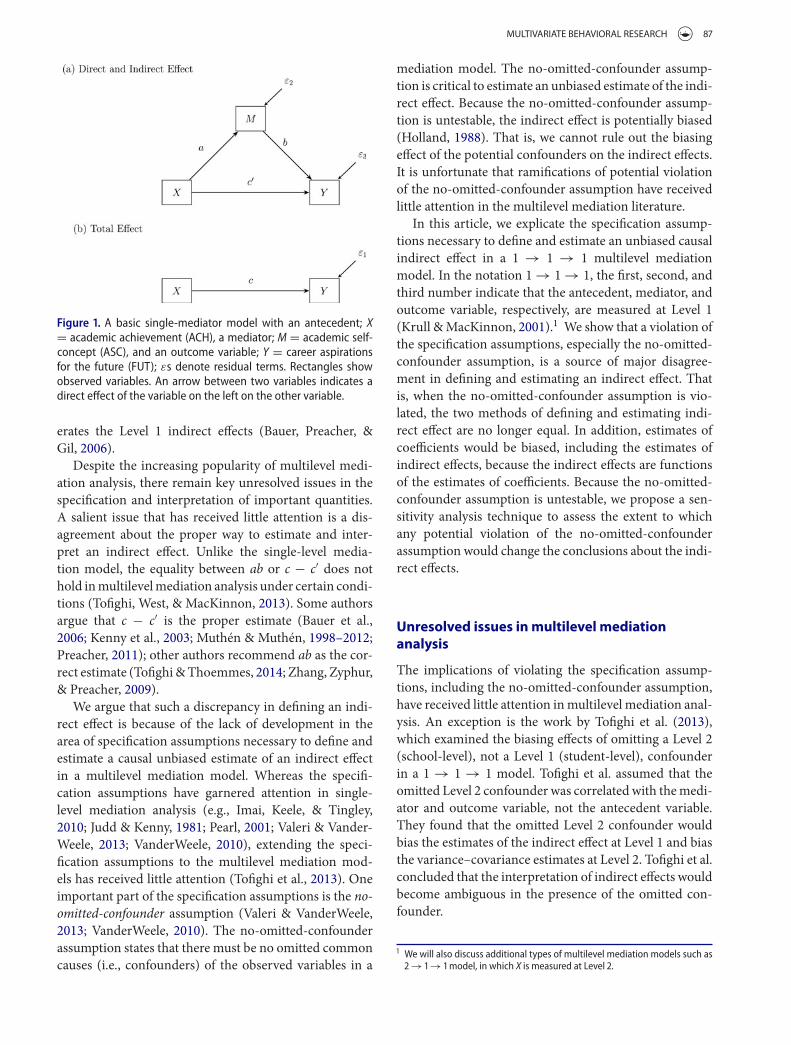


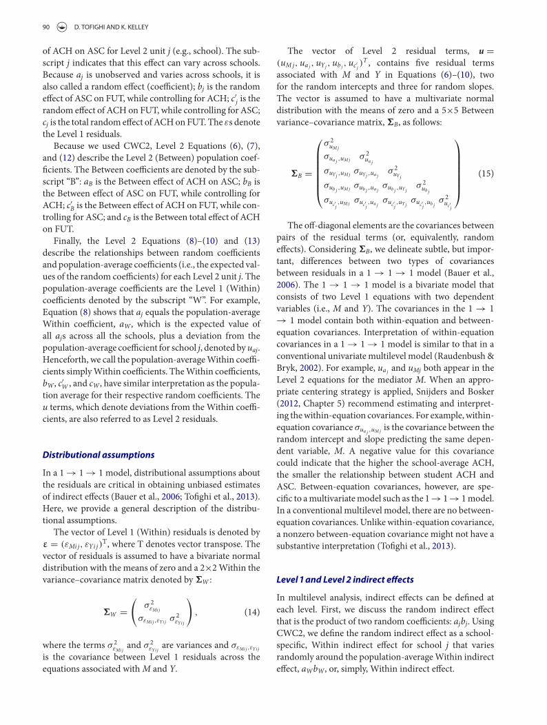
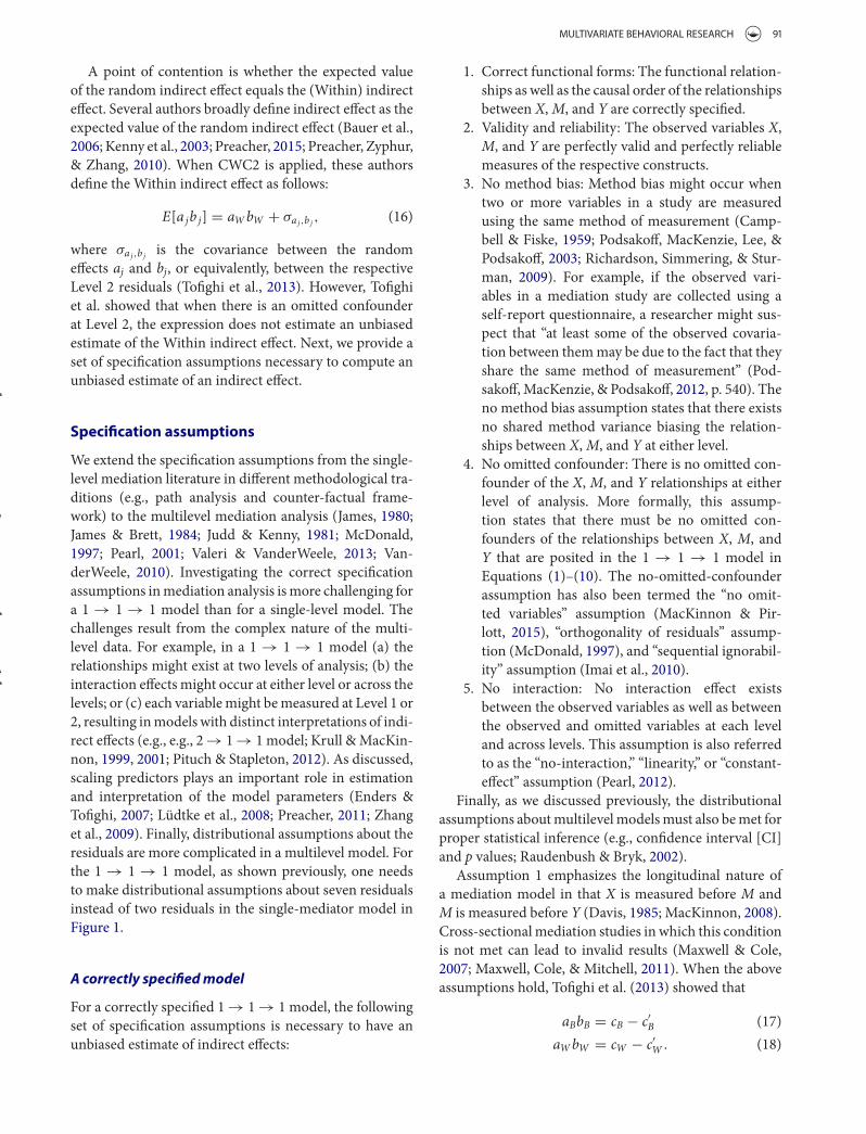
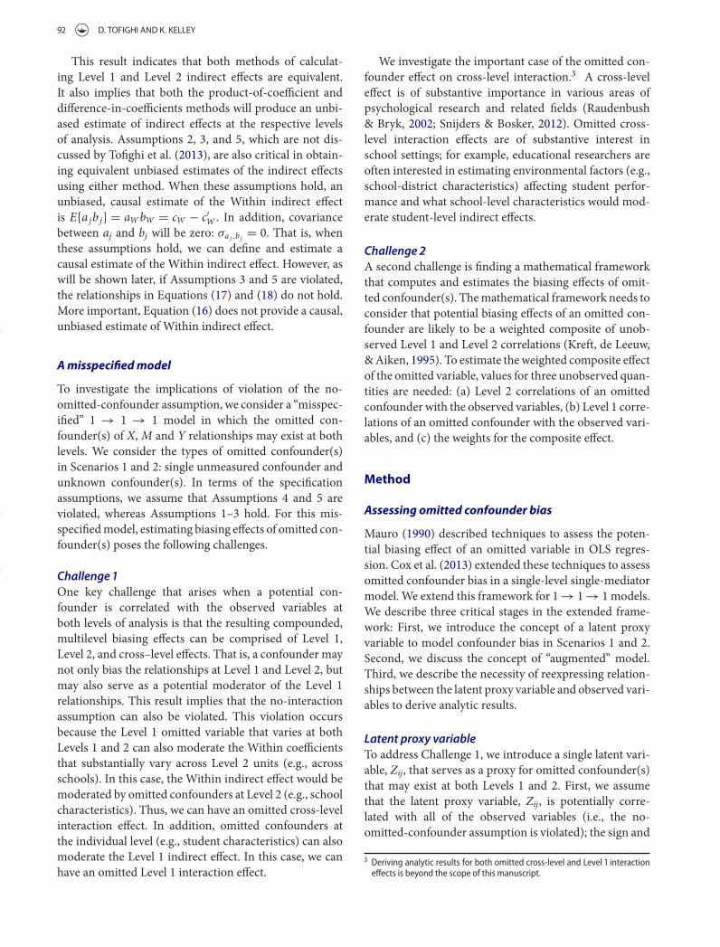

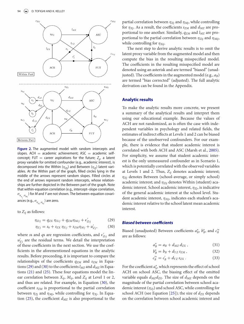

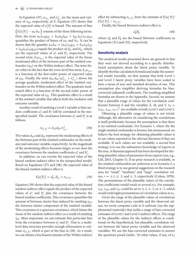
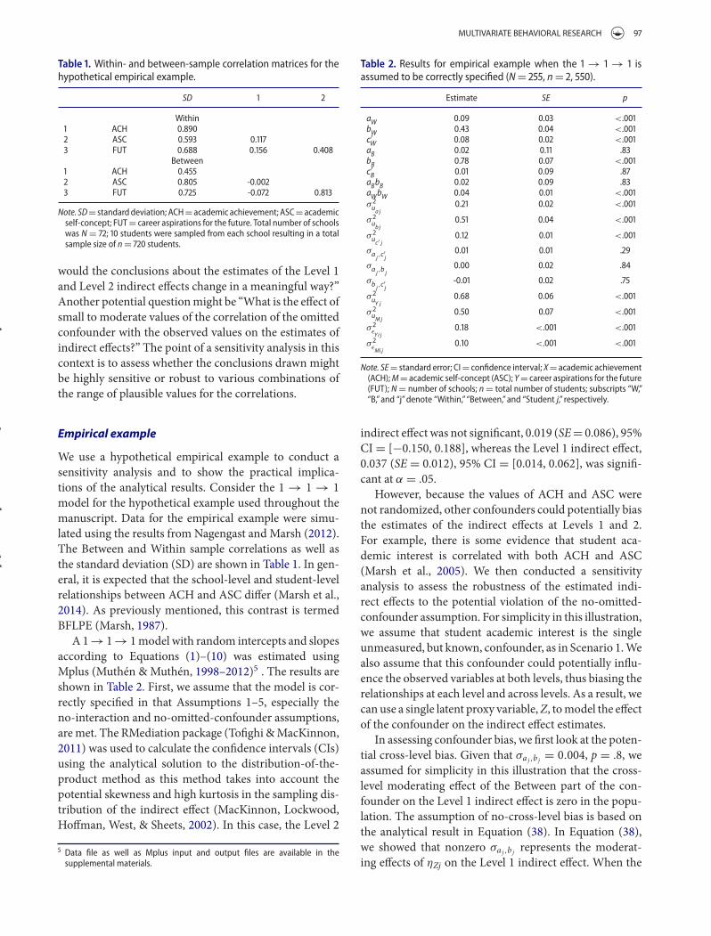

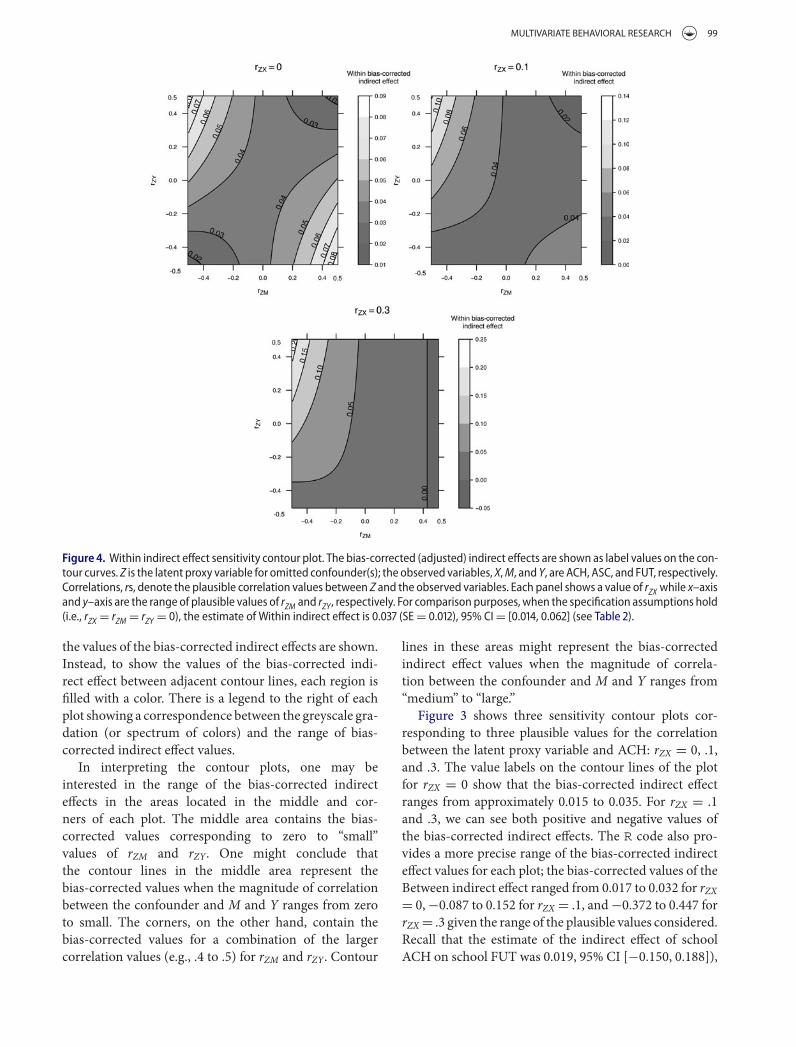


![· Web viewDischarge all prior parenting orders with respect to the children of the relationship: [X] born [omitted] 2005; [Y] born [omitted] 2007; and [Z] born [omitted] 2010.](https://static.documents.pub/doc/80x56/5fb14f41e9ac203ba6294d37/web-view-discharge-all-prior-parenting-orders-with-respect-to-the-children-of-the.jpg)


