59
Djoni Hartono Assessing policy effectiveness during the crisis: The case of Indonesia

Djoni Hartono
Assessing policy effectiveness during the crisis: The case of Indonesia

The International Institute for Labour Studies was established in 1960 as an autonomous facility of the International Labour Organization (ILO). Its mandate is to promote policy research and public discussion on issues of concern to the ILO and its constituents — government, business and labour. The Discussion Paper Series presents the preliminary results of research undertaken by or for the IILS. The documents are issued with a view to eliciting reactions and comments before they are published in their final form.

Assessing policy effectiveness during the
crisis: The case of Indonesia
Djoni Hartono
INTERNATIONAL LABOUR ORGANIZATION
INTERNATIONAL INSTITUTE FOR LABOUR STUDIES
Copyright © International Labour Organization (International Institute for Labour Studies) 2011. Short excerpts from this publication may be reproduced without authorization, on condition that the source is indicated. For rights of reproduction or translation, application should be made to the Editor, International Institute for Labour Studies, P.O. Box 6, CH-1211 Geneva 22 (Switzerland). ISBN Print: 978-92-9014-980-4 Web/pdf: 978-92-9014-981-1 First published 2011 The responsibility for opinions expressed in this paper rests solely with its author, and its publication does not constitute an endorsement by the International Institute for Labour Studies of the opinions expressed. Requests for this publication should be sent to: IILS Publications, International Institute for Labour Studies, P.O. Box 6, CH-1211 Geneva 22 (Switzerland).
Table of Contents
Abbreviations .............................................................................................................................. i Executive summary ................................................................................................................... 1
Chapter 1 Introduction ........................................................................................................... 3 Chapter 2 Research methodology........................................................................................... 5
2.1. Basic methodology of a Social Accounting Matrix (SAM) ....................................... 5 2.1.1. A basic framework of SAM ........................................................................... 5
2.1.2. The derivation of accounting multiplier matrix and employment multiplier matrix ........................................................................................................................ 6 2.2. Dynamic Social Accounting Matrix (DySAM) .......................................................... 7 2.2.1. Description of DySAM .................................................................................. 7 2.2.2. Technical framework of DySAM ................................................................... 7
Chapter 3 Crisis overview ....................................................................................................... 9 3.1. Indonesian economic performance prior to and during the 1997 Asian Financial Crisis ........................................................................................................ 9
3.2. Indonesian economic performance prior to and during the 2008 Global Economic Crisis ................................................................................................................ 10 3.3. The Government of Indonesia’s response to the crisis .............................................. 11 3.3.1. Maintain and improve people purchasing power .......................................... 12 3.3.2. Prevent employee’s contract termination and improvement on product competitiveness ....................................................................................................... 12 3.3.3. Program on infrastructures ............................................................................ 12
Chapter 4 Analysis of employment data .............................................................................. 13 4.1. Overview of Economic Growth and Employment by Sector .................................... 13 4.2. Overview of the estimation of employment in the official Indonesian SAM 2005 ... 14 4.3. Overview of the methodology used to construct the employment satellite of the DySAM ................................................................................................................... 16 4.4. Estimation of labour productivity based on DySAM ................................................ 16
4.5. Comparative analysis of two employment data sets (Labour Force Survey / DySAM versus SAM) .................................................................................................................... 18
4.6. Recommendations for estimation of employment for the DySAM employment satellite account........................................................................................... 19 4.7. New employment estimates derived for the DySAM employment satellite account for 2005 - 2008 ................................................................................................................. 19 4.8. New labour productivity estimates for 2005 -2008 ................................................... 21
Chapter 5 Simulation and results ......................................................................................... 23 5.1. Data on the realization rates of the fiscal stimulus .................................................... 23 5.2. Mapping of realization of fiscal stimulus budget on Indonesian SAM classification for each instrument ........................................................................................................... 24 5.3. List of possible scenarios on DySAM analysis ......................................................... 25
5.4. The impact of fiscal stimulus on Indonesian economic performance ....................... 26 5.4.1. Output and Employment by Sector ............................................................... 26 5.4.2. The impact of each fiscal stimulus instrument on production activities ....... 26 5.4.3. The impact of each fiscal stimulus instrument on labour income ................ 29 5.4.4. The impact of each fiscal stimulus instrument on household income .......... 32 5.4.5.The impact of each fiscal stimulus instrument on employment .................... 33 5.5. The net cost of the fiscal stimulus ............................................................................. 39
Chapter 6 Conclusion ............................................................................................................ 40 Chapter 7 Policy implication................................................................................................. 41 Annex 1: Indonesian Economic Performance before and during the Crisis ............................ 42 Annex 2: Labour Composition before and during the Crisis ................................................... 43 Annex 3: Informality by Sector before and during the Crisis .................................................. 43 Annex 4: Government Fiscal Stimulus 2009 (billion IDR) .................................................... 44 Annex 5: New Estimates of Employment ................................................................................ 46 Annex 6: New Estimates of Productivity................................................................................. 47 Annex 7:Tax Cut Instrument on Fiscal Stimulus by SAM Classification (in billion IDR) .... 48
References .............................................................................................................................. 49

i
Abbreviations BPS Badan Pusat Statistik (Central Agent of Statistics) DySAM Dynamic SAM FSP Fiscal Stimulus Policy GDP Gross Domestic Product GoI Government of Indonesia ILO International Labour Organization IO Input – Ouput KHM Kebutuhan Hidup Minimum (consumption at the minimum level) KILM Key Indicators of The Labor Market KUR Kredit Usaha Rakyat (people credit program) LFS Labour Force Survey MSME Micro, Small, Medium Enterprises NTP Nilai Tukar Petani (farmer trade index) PNPM Program Nasional Pemberdayaan Masyarakat (national program for community
development PTKP Pendapatan Tidak Kena Pajak (level of income that is not accounted in the tax) SAM Social Accounting Matrix UMR Upah Minimum Regional (regional minimum wage) VAT Value Added Tax
Assessing policy effectiveness during the crisis: The case of Indonesia DP 208
1
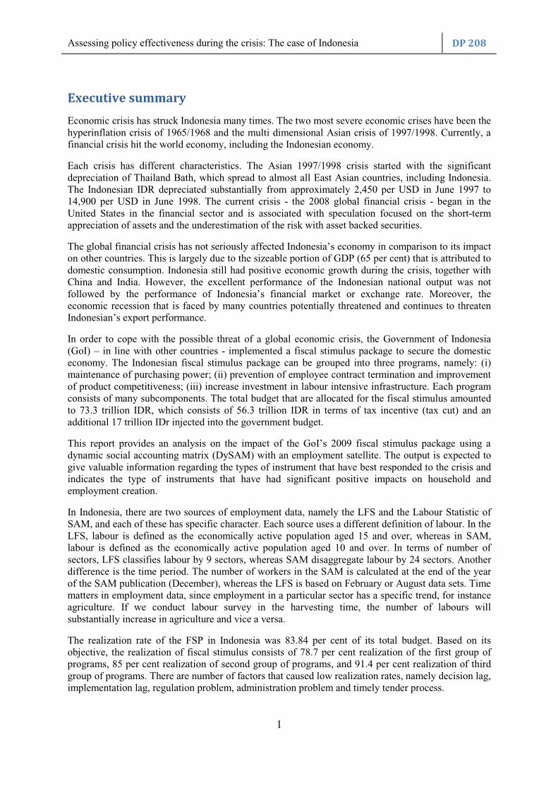
Executive summary
Economic crisis has struck Indonesia many times. The two most severe economic crises have been the hyperinflation crisis of 1965/1968 and the multi dimensional Asian crisis of 1997/1998. Currently, a financial crisis hit the world economy, including the Indonesian economy.
Each crisis has different characteristics. The Asian 1997/1998 crisis started with the significant depreciation of Thailand Bath, which spread to almost all East Asian countries, including Indonesia. The Indonesian IDR depreciated substantially from approximately 2,450 per USD in June 1997 to 14,900 per USD in June 1998. The current crisis - the 2008 global financial crisis - began in the United States in the financial sector and is associated with speculation focused on the short-term appreciation of assets and the underestimation of the risk with asset backed securities.
The global financial crisis has not seriously affected Indonesia’s economy in comparison to its impact on other countries. This is largely due to the sizeable portion of GDP (65 per cent) that is attributed to domestic consumption. Indonesia still had positive economic growth during the crisis, together with China and India. However, the excellent performance of the Indonesian national output was not followed by the performance of Indonesia’s financial market or exchange rate. Moreover, the economic recession that is faced by many countries potentially threatened and continues to threaten Indonesian’s export performance.
In order to cope with the possible threat of a global economic crisis, the Government of Indonesia (GoI) – in line with other countries - implemented a fiscal stimulus package to secure the domestic economy. The Indonesian fiscal stimulus package can be grouped into three programs, namely: (i) maintenance of purchasing power; (ii) prevention of employee contract termination and improvement of product competitiveness; (iii) increase investment in labour intensive infrastructure. Each program consists of many subcomponents. The total budget that are allocated for the fiscal stimulus amounted to 73.3 trillion IDR, which consists of 56.3 trillion IDR in terms of tax incentive (tax cut) and an additional 17 trillion IDr injected into the government budget.
This report provides an analysis on the impact of the GoI’s 2009 fiscal stimulus package using a dynamic social accounting matrix (DySAM) with an employment satellite. The output is expected to give valuable information regarding the types of instrument that have best responded to the crisis and indicates the type of instruments that have had significant positive impacts on household and employment creation.
In Indonesia, there are two sources of employment data, namely the LFS and the Labour Statistic of SAM, and each of these has specific character. Each source uses a different definition of labour. In the LFS, labour is defined as the economically active population aged 15 and over, whereas in SAM, labour is defined as the economically active population aged 10 and over. In terms of number of sectors, LFS classifies labour by 9 sectors, whereas SAM disaggregate labour by 24 sectors. Another difference is the time period. The number of workers in the SAM is calculated at the end of the year of the SAM publication (December), whereas the LFS is based on February or August data sets. Time matters in employment data, since employment in a particular sector has a specific trend, for instance agriculture. If we conduct labour survey in the harvesting time, the number of labours will substantially increase in agriculture and vice a versa.
The realization rate of the FSP in Indonesia was 83.84 per cent of its total budget. Based on its objective, the realization of fiscal stimulus consists of 78.7 per cent realization of the first group of programs, 85 per cent realization of second group of programs, and 91.4 per cent realization of third group of programs. There are number of factors that caused low realization rates, namely decision lag, implementation lag, regulation problem, administration problem and timely tender process.
Assessing policy effectiveness during the crisis: The case of Indonesia DP 208
2
Overall, all the FSP instruments have has a positive impact on Indonesian macroeconomic indicators, namely sectoral output, labour income, household income and employment by location and gender. One of the FSP instruments is personal income tax reduction. This instrument had a larger impact on production activities in almost all sectors, except for infrastructure sectors, such as labour and capital intensive roads, irrigation and the rest of the construction sector. It is important to note here that the total budget that is spent through this scenario was substantial - as much as 24.7 trillion IDR. According to the results of the simulations, the five sectors that will experience the highest impact are livestock, fishery, crops, restaurant and food, drink and tobacco sectors. It is expected that labour in the crops sector seems to benefit the most in any scenario. In terms of occupation, agriculture worker and manual worker is expected to received the largest impact. Since the structure of employment in Indonesia is majorly dominated by informal worker and mostly are men, the impact of fiscal stimulus is expected to biased to informal worker particularly on men worker.
It is worth noting that estimating the impact of the fiscal stimulus policy by using DySAM approach in this study has some limitations Those limitations are (i) the method does not address the price issue; (ii) structure of sectors in DySAM are not detail. This cause a relatively low precision on the mapping procedure; (iii) all shocks or injections are placed in exogenous matrix, thus the impact of each shock is simply the product of exogenous matrix and multiplier matrix. Since the multiplier matrix are the same for all scenarios, the impact of tax changes, tariff income changes, subsidy changes, and others shock on particular account with the same value will be treated the same and the result will be the same in magnitude. In other words, as long as we satisfy above condition, all fiscal stimulus instrument will have same multiplier effect.

Assessing policy effectiveness during the crisis: The case of Indonesia DP 208
3
Chapter 1 Introduction
Indonesia has been struggling with many crises, including economic crises. Since independence in 1945, the two most destructive crises have been the hyperinflation crisis of 1965/1968 and the multi dimensional Asian crisis of 1997/1998. The latter one changed Indonesia substantially.
The Asian 1997/1998 crisis started with the significant depreciation of the Thailand Bath, which spread to almost all East Asian countries, including Indonesia. The Indonesian IDR depreciated substantially from approximately 2,450 per USD in June 1997 to 14,900 per USD in June 1998 (Islam and Chowdhury, 2009:140). These conditions subsequently put substantial pressure on Indonesian’s economic performance, especially for producers who largely depended on imported commodities and foreign debt. From on annual average of seven percentage points, growth declined by nearly 14 percentage points in 1998. Consequently, many firms went bankrupt and this created severe loss of employment in the formal sector, and many formal workers were pushed into self-employment in the agricultural and informal economy. Churning in the labour market was high, with 30 per cent of male workers and 40 per cent of female workers changing sectors between 1997 and 1998 (World Bank, 2010:36). Moreover, the inflation rate grew to 38 per cent in the first semester of 1998 and caused a significant drop in real income (Bank of Indonesia, 1999:11). People began to lose faith in the currency and this caused a ‘run on’ many banks, particularly large-scale private banks (Bank Central Asia). As a result, 16 private banks were liquidated. The combination of the crisis of the exchange rate, destabilization of the banking sector and high inflation caused an economic collapse, which then triggered a social and politic crisis. Massive demonstrations across the country demanded that the President resign.
In the period after the crisis, price stabilization policies were adopted and Growth Domestic Product (GDP) growth averaged 4.7 percentage points between 1999 and 2003, largely due to rapid growth in minerals and crude oil exports (World Bank, 2010; Islam and Chowdhury, 2009). However, economic recovery was characterized by jobless growth and labour market participation decreased as the number of discouraged workers increased.
In 2008, a crisis, now known as ‘the global financial crisis’, hit the world economy. This crisis has different characteristics than the previous 1997/1998 Asian economic crisis. The global financial crisis began in United States in the financial sector and is associated with speculation focused on the short-term appreciation of assets and the underestimation of the risk of asset backed securities. The underestimation of risk translated to the relaxation of lending practices, which saw credit made available to riskier segments of the market - the so-called ‘sub-prime’ loans market. The assumption was that housing prices would remain stable and that options for re-financing on the basis of increasing property values would remain available. However, in 2006 housing prices began to deteriorate, which undermined equity and thus exposed risk, subsequently foreclosures began to rise. This undermined the value of financial assets based on these mortgages (mortgage backed securities), which had been given investment grade status by credit rating agencies. Concurrently, insurance provided in the speculative market through credit default swaps, which offered holders a guarantee against loan default, were also written against many of these risky mortgage loans. As a result, many financial insurance providers were unable to honour their obligations.
Economies the world over saw high levels of uncertainty, declining asset values and falling consumer demand, as the implications of failure in global financial sector began to manifest. The economic down turn has had implications for employment and progress towards poverty reduction the world over. Analysis from the International Labour Organization (ILO) Key Indicators of the Labour Market (KILM) indicates that between 2007 and 2009 up to 61 million additional people may have fallen into unemployed and up to 222 million additional workers are likely to fall into extreme poverty (ILO, 2010).

Assessing policy effectiveness during the crisis: The case of Indonesia DP 208
4
The crisis saw governments in developed and developing countries step in to prevent the collapse of the financial sector, in an attempt to restore confidence and circumvent the subsequent impact that recessions have on enterprise and households. Many governments launched job creation programs and targeted cash transfer programs. Interest rates were lowered in many countries in an attempt to improve lending conditions.
In comparison to other countries, the global financial crisis has not seriously affected Indonesia’s economy, largely due to the sizeable portion of GDP (65 per cent) that is attributed to domestic consumption. Indonesia still had positive economic growth during the crisis, together with China and India. In 2008, the Indonesian economy grew 6.1 per cent relative to previous year and then grew slower by 4.5 per cent in 2009 (Central Bank of Indonesia, 2010:29). Even though the Indonesian growth declined in 2009, in the first semester of 2010 it has shown strong signs of recovery, with growth at 5.9 percentage points (Central Agency of Statistics, 2010:1).
The excellent performance of the Indonesian national output was not followed by the performance of Indonesian financial market and exchange rate. The Jakarta Stock Exchange Index dropped nearly 50 per cent in January 2009 in comparison to January 2008. These conditions implied a massive capital outflow that negatively affected Indonesia’s economic performance. In the second quarter of 2009, the performance of the financial market started to recover, as investor confidence increased. At the end of 2009, the Jakarta Stock Exchange Index achieved a significantly higher level, at 2,534 relative to the level in the end 2008 that was only achieved 1,355 (Central Bank of Indonesia, 2010:24). A similar condition was also experienced by Indonesian exchange rate market. The IDR fluctuated during the crisis and declined to 12,150 per USD in November 2008 (Bank of Indonesia, 2009:5). The exchange rate performance began to improve from the second quartile of 2009. The IDR appreciated to 9,425 per US dollar by the end of 2009 (Bank of Indonesia, 2010:26).
Despite the fact that the Indonesian economy still performed better than other countries during the crisis, the economic recession that is faced by many countries potentially threatens Indonesian’s export performance. In line with other Asian countries, Indonesia’s export decreased due to lower demand particularly from other developed countries (Bank of Indonesia, 2010:24). Trade surplus that has existed for several years decreased from 32.7 billion USD in 2007 to 23.3 billion USD in 2008. Even though export performance has deteriorated, strong domestic demand provided a buffer and offset the negative impact of weaker performance of export (Ziegenhain, 2010:1). The crisis also potentially threaten Indonesian labour market which dominated by informal sector. If the business collapse, many workers will be drawn to informal sector and increase the Indonesian informality rate. A report by World Bank (2010) found that informal workers have a significantly less income than formal workers. Thus. It is also expected that poverty rate will increase as well as the informality rate.
In order to cope with the possible threats of global economic crisis, Government of Indonesia (GoI) implemented a fiscal stimulus package to secure domestic economy. Those polices can be grouped into three programs, namely:
1. maintenance of purchasing power;
2. prevent employee’s contract termination and improvement on product competitiveness;
3. enhanced infrastructure investment.
Each program consists of many subcomponents. Together they are expected to minimize the impact of global financial crisis on Indonesian economic performance and support employment creation.
This report provides valuable analysis on the types of instruments that have best responded to the crisis and indicates the type of instruments that have had significant positive impacts on household and employment creation. The instrument that is primarily used to undertake this analysis is a dynamic social accounting matrix, which was developed to analyze the impact and cost-effectiveness of government investments, such as those associated with the GoI’s 2009 fiscal stimulus package.

Assessing policy effectiveness during the crisis: The case of Indonesia DP 208
5
Section 1 of this report presents the introduction, which explains the background of the study. Section 2 describes research methodology. Section 3 presents the crisis overview and followed by an analysis of employment data in Section 4. The simulation and results are provided in section 5. Finally, the conclusion and policy implication are finally drawn in section 6 and section 7.
Chapter 2: Research methodology 2.1. Basic methodology of a Social Accounting Matrix (SAM) 2.1. 1. A basic framework of SAM
SAM is a double entry of traditional economic accounting, shaped partition matrix that records all economic transactions between agents, particularly among the sectors in the production block, institutions blocks (including households), and in the sectors of production factors (Pyatt and Round, 1979; Sadoulet and de Janvry, 1995; Hartono and Resosudarmo, 1998). As a data collection system, it is comprehensive and has many benefits. A SAM summarizes all the activities of transactions in an economy within a particular period of time (usually one year), thus providing a general overview of the socio-economic structure in an economy and describes the situation of income distribution.
SAM is also an important analytical tool, because: (1) through the concept of the multiplier, the SAM can show the impact of economic policy on household income and income distribution; and (2) application is relatively simple and thus comparatively easily applied.
Figure 2.1. SAM Framework
A. E X P E N D I T U R E
Endogenous Accounts Exogenous Account
TOTAL Production Factors
Institutions Production Activities
R E C E I P T S
Endogenous
Accounts
Production Factors
0
0
T13
Z1
y1
Institutions
T21
T22
0
Z2
y2
Production Activities
0
T32
T33
Z3
y3
Exogenous Account
T41
T42
T43
Z4
z
TOTAL y’1 y’2 y’3 z’
The basic framework of a SAM is a partition matrix with 4x4 dimensions, as shown in Figure 2.1. In general, the accounts in a SAM are grouped into endogenous and exogenous accounts.1 Endogenous accounts in a SAM are the main accounts, consisting of three blocks, namely: production factors, institutions and production activities. The row shows income, while the column shows expenditure. Sub-matrix Tij shows the income of the account in row i from the account of column j. Vector yi shows the total incomes of the account in row i, otherwise vector y′′′′j shows the total expenditure of the account in column j. In addition, SAM requires that the vector yi is the same with vector y′′′′j, in other words y′′′′j is a transpose of yi, for every i = j. Relationship contained in Figure 2.1 can be written in matrix form as (Defourny and Thorbecke, 1984): 1 Endogenous account is parts of SAM account that its values are determined by products of accounting multiplier matrix and exogenous account. Exogenous account is previously determined and use as injection to give impact on endogenous account.

Assessing policy effectiveness during the crisis: The case of Indonesia DP 208
6
y Ay x= + [1]
where:
y is the vector of total income
x is the vector whose members are expressed by m mnnx z=∑ where mn iz Z∈
A is the matrix whose members are expressed by mn mn na t y= where mn ijt T∈ and n jy y′∈
2.1.2. The derivation of an accounting multiplier matrix and an
employment multiplier matrix
The accounting multiplier matrix within the framework of a SAM is very important, because the matrix can capture the full impact of the change in a sector across other sectors in the economy and can also be used to explain the impact that occurs in the endogenous accounts caused by changes in exogenous accounts. This matrix is a multiplier matrix, which is common and frequently used for economic analysis. The accounting multiplier matrix is basically a standard form of the inverse matrix of the , and can be derived from the basic framework of the SAM and expressed as (Defourny and Thorbecke, 1984):
1( ) ay Ay x y Ay x y I A x y M x−= + ⇔ − = ⇔ = − ⇔ = [2]
The accounting multiplier matrix or aM is a matrix that informs of the overall impact of changes
given to a particular sectorand how this transmits to other sectors after going through the entire system in the SAM. The accounting multiplier matrix is used to simulate the effect of stimulus on the economy, especially on household income and production activities. Furthermore, to see the impact of stimulus on labour, an employment multiplier matrix can be developed. An employment multiplier matrix is derived from the following equation:
L By= [3]
where:
B is the diagonal matrix whose membership represents the ratio between labour and output (employment-output share matrix).
L is the vector whose members are the sectoral employment.
If equation [1] and [2] substituted into equation [3], equation [3] can also be written as:
1( ) ( ) aL By L B Ay x L B I A x L BM x−= ⇔ = + ⇔ = − = = [4]
where:
aBM is the employment multiplier matrix
The employment multiplier matrix or is a matrix that shows the overall impact of changes in employment within and across production activities after going through the entire system in the SAM. The employment multiplier matrix is used to simulate the effect of stimulus on employment.
Assessing policy effectiveness during the crisis: The case of Indonesia DP 208
7
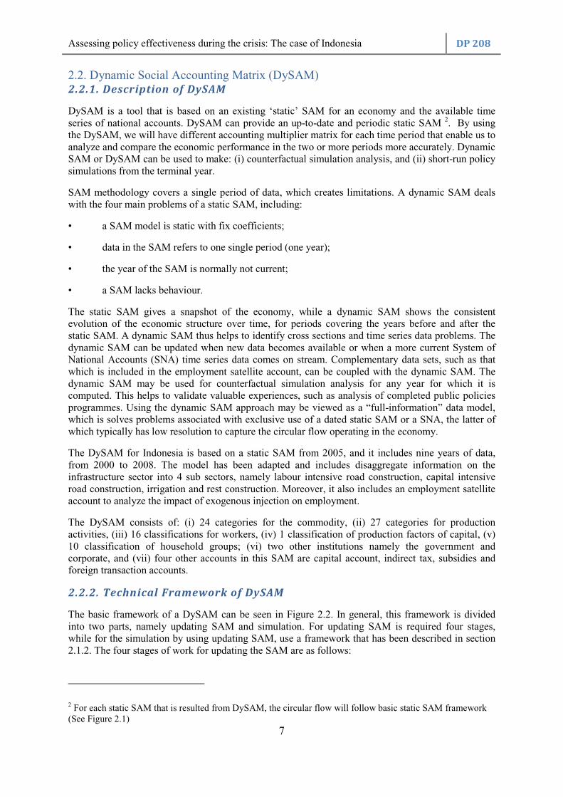
2.2. Dynamic Social Accounting Matrix (DySAM) 2.2.1. Description of DySAM
DySAM is a tool that is based on an existing ‘static’ SAM for an economy and the available time series of national accounts. DySAM can provide an up-to-date and periodic static SAM 2. By using the DySAM, we will have different accounting multiplier matrix for each time period that enable us to analyze and compare the economic performance in the two or more periods more accurately. Dynamic SAM or DySAM can be used to make: (i) counterfactual simulation analysis, and (ii) short-run policy simulations from the terminal year.
SAM methodology covers a single period of data, which creates limitations. A dynamic SAM deals with the four main problems of a static SAM, including:
• a SAM model is static with fix coefficients;
• data in the SAM refers to one single period (one year);
• the year of the SAM is normally not current;
• a SAM lacks behaviour.
The static SAM gives a snapshot of the economy, while a dynamic SAM shows the consistent evolution of the economic structure over time, for periods covering the years before and after the static SAM. A dynamic SAM thus helps to identify cross sections and time series data problems. The dynamic SAM can be updated when new data becomes available or when a more current System of National Accounts (SNA) time series data comes on stream. Complementary data sets, such as that which is included in the employment satellite account, can be coupled with the dynamic SAM. The dynamic SAM may be used for counterfactual simulation analysis for any year for which it is computed. This helps to validate valuable experiences, such as analysis of completed public policies programmes. Using the dynamic SAM approach may be viewed as a “full-information” data model, which is solves problems associated with exclusive use of a dated static SAM or a SNA, the latter of which typically has low resolution to capture the circular flow operating in the economy.
The DySAM for Indonesia is based on a static SAM from 2005, and it includes nine years of data, from 2000 to 2008. The model has been adapted and includes disaggregate information on the infrastructure sector into 4 sub sectors, namely labour intensive road construction, capital intensive road construction, irrigation and rest construction. Moreover, it also includes an employment satellite account to analyze the impact of exogenous injection on employment.
The DySAM consists of: (i) 24 categories for the commodity, (ii) 27 categories for production activities, (iii) 16 classifications for workers, (iv) 1 classification of production factors of capital, (v) 10 classification of household groups; (vi) two other institutions namely the government and corporate, and (vii) four other accounts in this SAM are capital account, indirect tax, subsidies and foreign transaction accounts.
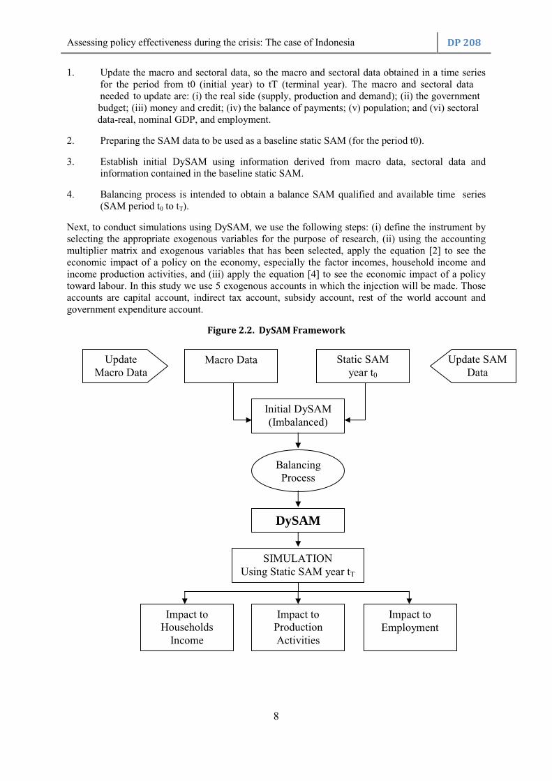
2.2.2. Technical Framework of DySAM
The basic framework of a DySAM can be seen in Figure 2.2. In general, this framework is divided into two parts, namely updating SAM and simulation. For updating SAM is required four stages, while for the simulation by using updating SAM, use a framework that has been described in section 2.1.2. The four stages of work for updating the SAM are as follows:
2 For each static SAM that is resulted from DySAM, the circular flow will follow basic static SAM framework (See Figure 2.1)
Assessing policy effectiveness during the crisis: The case of Indonesia DP 208
8
1. Update the macro and sectoral data, so the macro and sectoral data obtained in a time series for the period from t0 (initial year) to tT (terminal year). The macro and sectoral data needed to update are: (i) the real side (supply, production and demand); (ii) the government budget; (iii) money and credit; (iv) the balance of payments; (v) population; and (vi) sectoral data-real, nominal GDP, and employment.
2. Preparing the SAM data to be used as a baseline static SAM (for the period t0).
3. Establish initial DySAM using information derived from macro data, sectoral data and information contained in the baseline static SAM.
4. Balancing process is intended to obtain a balance SAM qualified and available time series (SAM period t0 to tT).
Next, to conduct simulations using DySAM, we use the following steps: (i) define the instrument by selecting the appropriate exogenous variables for the purpose of research, (ii) using the accounting multiplier matrix and exogenous variables that has been selected, apply the equation [2] to see the economic impact of a policy on the economy, especially the factor incomes, household income and income production activities, and (iii) apply the equation [4] to see the economic impact of a policy toward labour. In this study we use 5 exogenous accounts in which the injection will be made. Those accounts are capital account, indirect tax account, subsidy account, rest of the world account and government expenditure account.
Figure 2.2. DySAM Framework
Update Macro Data
Macro Data Static SAM year t0
Update SAM Data
Initial DySAM (Imbalanced)
Balancing Process
DySAM
SIMULATION Using Static SAM year tT
Impact to Employment
Impact to Production Activities
Impact to Households
Income
Assessing policy effectiveness during the crisis: The case of Indonesia DP 208
9
Chapter 3: Crisis overview 3.1. Indonesian economic performance prior to and during the 1997 Asian Financial Crisis
Prior to the 1997 Asian Financial crisis, Indonesia was one of the emerging economies in Asia. GDP grew positively at between seven to nine per cent per year from 1990 onwards. During the same period, the unemployment rate was on average 4.89 per cent. In 1990 approximately 45 per cent of the labour force worked in the agricultural sector (World Bank, 2010). In terms of the inflation rate, Indonesia experienced a relatively stable inflation rate on the level of 8.1 per cent (year on year / yoy).
One year before the 1997 Asian Financial crisis, Indonesia’s economic performance was healthy. The national output grew by 7.8 per cent, the inflation rate was at an acceptable level of an average of 6.6 per cent and the unemployment rate was on average 4.89 per cent. In terms of labour composition, 43 per cent of the labour force was employed in agricultural sector, followed by trade, restaurant and hotel sectors which employed approximately 19 per cent of workers. Approximately 14 per cent were employed in the services sector and 13 per cent in the manufacturing sector. The agricultural sector was the most dominant sector in terms of labour absorption, but the percentages of workers who worked in this sector decreased continuously from 56 per cent in 1990 to approximately 44 per cent in 1996 (Central Agency of Statistics, 2009; World Bank, 2010). This implies that employment in Indonesia started to move from the primary sector to the secondary and tertiary sector (the detail figure can be found in Annex 1 and Annex 2).
In 1997 Indonesian output grew positively by 7.4 per cent in the first quartile, 6.1 per cent in the second quartile and 4.5 per cent in the third quartile. Then, in the fourth quartile, Indonesian output contracted by -0.9 per cent - mostly due to the collapse of the manufacturing sector. The condition became worse in the next period, which saw output drop significantly to -19.4 per cent in the fourth quartile 1998. Indonesia entered into a recession and almost all sectors, except the agricultural sector experienced negative growth. The most affected sector was the banking sector that experienced the largest output drop by 43.5 per cent in the fourth quartile, followed by the construction sector (39.4 per cent) and the trade, hotel and restaurant sector (28.7 per cent).
The significant drop in growth was also accompanied by high inflation rate in 1997. Inflation rate increased up to the two digit level, amounting to 11.6 per cent. The decrease in the output and the higher inflation rate saw stagflation emerge in Indonesia. Inflation worsened in 1998 by as much as 77.6 per cent. It impacted on real income and purchasing power. In 1997, private consumption still grew positively by 5.9 per cent and in 1998 consumption dropped to -4.1 per cent.
The impact of the economic recession on employment was seen in severe loss of employment in the formal sector, and many formal workers were pushed into self-employment in the agricultural and informal sector. Due to the nature of poverty in Indonesia, the crisis was not reflected well in unemployment statistics, job destruction between sectors was however evident. For example, in 1998 the unemployment rate increased to 5.46 per cent from 4.68 per cent in 1997 (World bank, 2010). The number of workers who were employed in almost all sectors decreased except for agricultural sector and transportation sector. The worst case was in the manufacturing sector, followed by the construction sector, and trade, hotel and restaurant sector. The bankruptcy of many firms were triggering a wave of employee’ contract termination. Approximately 1.3 million of workers fell into unemployment due to contract termination in manufacturing sector. In the construction sector, approximately 678,000 workers lost their jobs followed by 406,000 others in trade, hotel and restaurant sector (Central Bank of Indonesia, 1999:38-39). Many newly unemployment workers switched to the informal economy or become entrepreneurs, with many workers turning to the agricultural sector. The agricultural sector created nearly 3.5 million new jobs in 1998. The expansion of the agricultural sector, along with the rise of the informal economy, minimized the impact of crisis on aggregate employment, but severely compromised employment quality. Total employment in 1998 was more than 87.6 million people or approximately 0.7 per cent higher than 1997. In terms of household income, real income decreased substantially even though the nominal wage increased.
Assessing policy effectiveness during the crisis: The case of Indonesia DP 208
10
This is largely due to the increasing number of workers who work in informal sector. On average the workers who work in informal sector are relatively earn less than formal sector and do not have any non-wage benefit (World Bank, 2010). As a result, more households received lower income than before and then increase the poverty level.
3.2. Indonesian economic performance prior to and during the 2008 Global Economic Crisis
After hit by the 1997 Asian Financial crisis, Indonesia has changed substantially economically, socially and politically. These changes caused a prolonging of the recovery period relative to other East Asian countries. Even now the economy has not returned to the pre-crisis growth levels. Since 2000 the Indonesian economy became more stable with the national output growing by between 5 per cent and 6 per cent per year. In 2007, Indonesia achieved 6.3 per cent on its output growth and moderate inflation rate by 11.6 per cent.
In terms of the labour market condition, the unemployment rate was higher than before, at 9.1 per cent in 2007. Based on data from Statistics Indonesia, the total labour force in August 2007 was equal to 109.9 million, which is 3.6 million higher than 2006 figures (4.69 per cent increase)(Central Agency of Statistics, 2008). The agricultural sector remained as the most dominant sector in terms of labour absorption, followed by trade sector and manufacturing sector. Indonesian labour market was dominated by informal labour, which was accounted approximately more than 70 per cent from total employment. In 2007, the number of people underemployed was high as much as 30.2 million or about 27.9 per cent from total labour force. (the detail figure can be found in Annex 1 and Annex 2).
In the first quartile of 2008, Indonesian growth was still positive and even larger than 2007. After that, output grew consistently by 6.2 and 6.3 per cent in the second and third quarters, and slightly slower at 5.27 per cent in the fourth quartile. In total, national output increased by 6.1 per cent in 2008. The decline in the growth rate, in comparison with 2007 levels, is attributed to lower growth in the manufacturing sector. The manufacturing sector experienced a quite difficult period, and Indonesian exports deteriorated from 10.63 per cent in first quartile up to 1.99 per cent in fourth quartile. Other sectors that also experienced slower growth are construction sector, trade sector and services sector.
The inflation rate in 2008 was quite high, at approximately 11.06 per cent. The consistent high inflation rate was mainly due to the increase of domestic oil prices and the price of world food crops. In May 2008 (Bank of Indonesia, 2009:5), GoI increased the domestic oil price by 28.7 per cent. Moreover, the scarcity of oil stock in some areas due to bad distribution also contributed to relatively higher inflation rate. The higher domestic oil price resulted in more expensive distribution costs. Thus, along with relatively higher prices of world food crops, the increase of the domestic oil price caused food commodity prices to rise much faster. In terms of labour statistics, the unemployment rate in 2008 was much lower than the previous year. The unemployment rate decreased from 9.11 per cent to 8.39 per cent of total labour force. Two sectors that are quite dominant in creating new job are services sector and trade sector. However, Informal labour still dominant and even increased in August 2008 relative to August 2007 (the detail figure can be found in Annex 3). In 2008, number of labourers who were underemployed also increased gradually up to 31.1 million people in August 2008 or about 27.8 per cent from total labour force. Underemployment and informal labour will move in the same direction since some persons who work less than its optimal rate (underemployment) can also be categorized as informal labour. The decrease of unemployment rate is understandable since more informal workers are employed in agricultural sector and transportation sector in line with the high output growth of those sectors. In this context, lower unemployment rate is not always a good news for the economy if the sectors that are improved are informal sector instead of formal sector. As we defined previously, workers in informal sector usually earn less than formal sector and do no received any non-wage benefit, such as insurance.
In the first quartile 2009, Indonesian national output grew by 4.53 per cent, which is much lower than the previous year. The second and third quarter continued to slow, with growth at 4.08 percentage
Assessing policy effectiveness during the crisis: The case of Indonesia DP 208
11
points and 4.16 per cent respectively. The decline in growth was mainly caused by the downturn in export performance due to world economic recession. In the fourth period, the economy showed signs of recovery, with growth at 5.43 per cent. The better economic growth in the last quartile 2009 was largely attributed to the recovery of manufacturing sector, which grew at approximately 4.16 per cent. The recovery was also supported by better performance of agricultural sector and construction sector. Accumulatively, the national output increased by 4.5 per cent in 2009. Even though the output grew slightly slower than a year before, Indonesia was one of the countries with best economic performance during the financial crisis, after China and India. One important determinant that successively prevented Indonesia from economic recession was the growth in domestic consumption. The general election and improvement in consumer confidence index contributed to the substantially high consumption growth by 5.95 per cent on average per annum. The fiscal stimulus package also supported this.
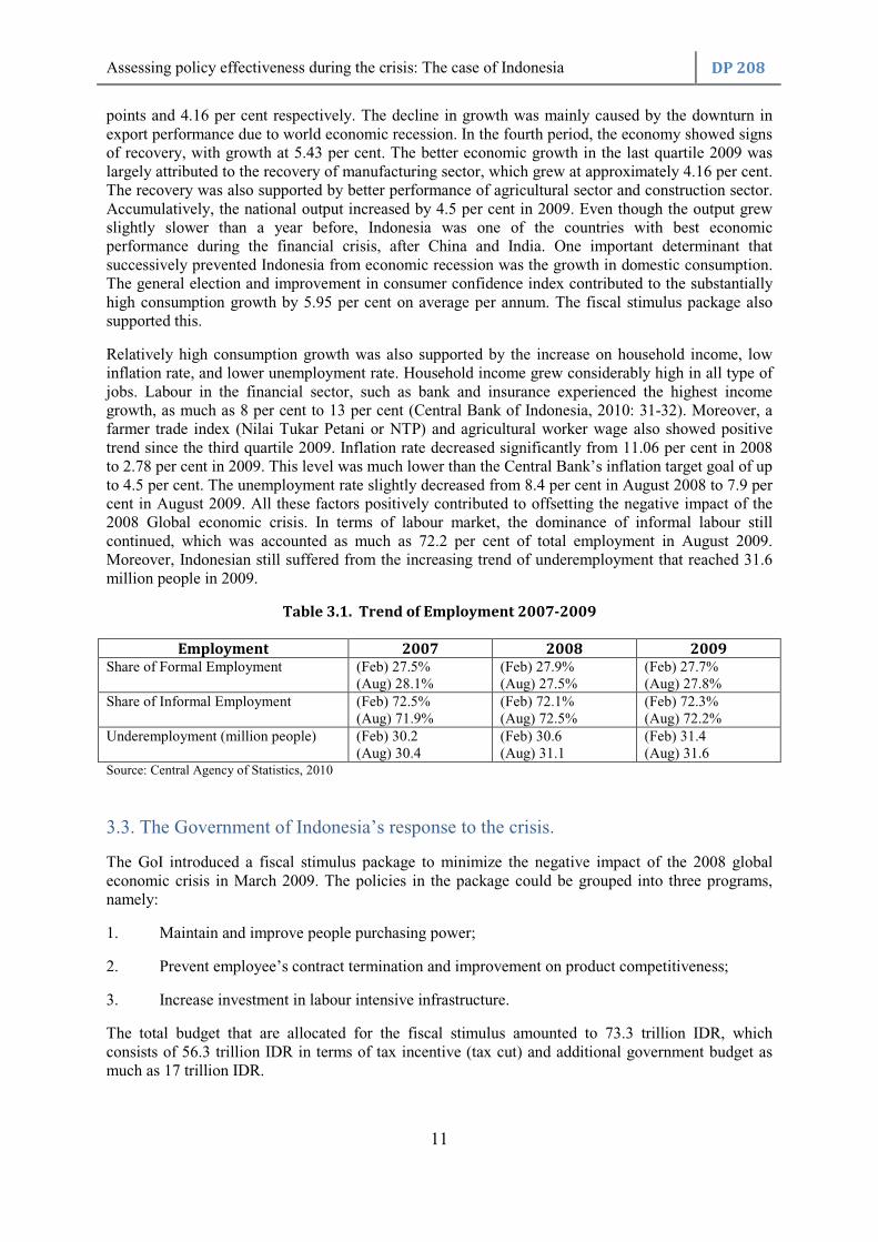
Relatively high consumption growth was also supported by the increase on household income, low inflation rate, and lower unemployment rate. Household income grew considerably high in all type of jobs. Labour in the financial sector, such as bank and insurance experienced the highest income growth, as much as 8 per cent to 13 per cent (Central Bank of Indonesia, 2010: 31-32). Moreover, a farmer trade index (Nilai Tukar Petani or NTP) and agricultural worker wage also showed positive trend since the third quartile 2009. Inflation rate decreased significantly from 11.06 per cent in 2008 to 2.78 per cent in 2009. This level was much lower than the Central Bank’s inflation target goal of up to 4.5 per cent. The unemployment rate slightly decreased from 8.4 per cent in August 2008 to 7.9 per cent in August 2009. All these factors positively contributed to offsetting the negative impact of the 2008 Global economic crisis. In terms of labour market, the dominance of informal labour still continued, which was accounted as much as 72.2 per cent of total employment in August 2009. Moreover, Indonesian still suffered from the increasing trend of underemployment that reached 31.6 million people in 2009.
Table 3.1. Trend of Employment 2007-2009
Employment 2007 2008 2009 Share of Formal Employment (Feb) 27.5%
(Aug) 28.1% (Feb) 27.9% (Aug) 27.5%
(Feb) 27.7% (Aug) 27.8%
Share of Informal Employment (Feb) 72.5% (Aug) 71.9%
(Feb) 72.1% (Aug) 72.5%
(Feb) 72.3% (Aug) 72.2%
Underemployment (million people) (Feb) 30.2 (Aug) 30.4
(Feb) 30.6 (Aug) 31.1
(Feb) 31.4 (Aug) 31.6
Source: Central Agency of Statistics, 2010
3.3. The Government of Indonesia’s response to the crisis.
The GoI introduced a fiscal stimulus package to minimize the negative impact of the 2008 global economic crisis in March 2009. The policies in the package could be grouped into three programs, namely:
1. Maintain and improve people purchasing power;
2. Prevent employee’s contract termination and improvement on product competitiveness;
3. Increase investment in labour intensive infrastructure.
The total budget that are allocated for the fiscal stimulus amounted to 73.3 trillion IDR, which consists of 56.3 trillion IDR in terms of tax incentive (tax cut) and additional government budget as much as 17 trillion IDR.
Assessing policy effectiveness during the crisis: The case of Indonesia DP 208
12
3.3.1. Maintain and improve people purchasing power
Consumption is one of the most important determinants of Indonesian economic growth, especially to prevent economic recession due to economic crisis. In order to maintain and improve purchasing power, the GoI utilized fiscal instruments, including tax and government expenditure. The Government reduced the individual tax rate, which resulted tax saving up to 24.5 trillion IDR. These tax saving policies consisted of two aspects, i.e. the reduction of tax rate for each group of household income and the increasing of level of income that is not accounted in the tax (Pendapatan Tidak Kena Pajak or PTKP). Each of those aspects contributed to as much as 13.2 trillion IDR and 15.8 trillion IDR additional savings respectively. By using a second instrument, government expenditure, the Government raised the subsidy for three commodities, namely cooking oil, bio-fuels and selected medicines. The Government spent approximately 1.35 trillion IDR on subsidies under the fiscal stimulus policies. Total fiscal stimulus aligned for the “Maintain and Improve People Purchasing Power” program was 25.8 trillion IDR. Overall, the objectives of this fiscal stimulus package are to mitigate the social impact and improve the income transfer. These can be reflected in some programs such as reduction of tax rate for each group of household income and the increasing of level of income that is not subject to tax (PTKP). (The detail figure can be found in Annex 4). 3.3.2. Prevent employee’s contract termination and improvement on
product competitiveness In order to improve domestic product competitiveness and increase the business resilience, the Government used three instruments, i.e. tax, subsidies and financing. Tax stimulus is given through the decreasing of corporate tax rate as much as 18.5 trillion IDR. In terms of subsidies, the government spent approximately 16.4 trillion IDR for tax and non tax subsidies. The tax subsidy consisted of the exemption of import duties, value added tax (VAT) on oil and gas exploration, income tax on geothermal and employee under the article 21. Meanwhile, the non-tax subsidies consisted of reduction of diesel fuel price, electricity price discount for industry, and interest rate subsidy for water companies. The last instrument that is used under this program was financing. Government gave capital investment for Askrindo and Jamkrindo to guarantee a ‘People Credit Program’ (Kredit Usaha Rakyat or KUR). The program is expected to increase the access of micro, small and medium enterprises (MSMEs) and cooperatives to financing sources. Total budget that were expected to spend under this program was 35.4 trillion IDR. (The detail figure can be found in Annex 4). Based on the details, each program has different sub objective. Corporate tax rate discount aims to save existing job, tax subsidy aims to improve income transfer and non-tax subsidy aims to mitigate the social impact that might occurred. 3.3.3. Increase investment in labour intensive infrastructure The GoI increased the total budget on infrastructure construction as much as 11.93 trillion IDR. The additional expenditure was accounted as much as 15 per cent of total government expenditure on infrastructure or 1.3 per cent of total Indonesian National Budget 2009. The highest share of infrastructure expenditure is allocated through Ministry of Public Works as
Assessing policy effectiveness during the crisis: The case of Indonesia DP 208
13
much as 6.6 trillion IDR. Sum of total government expenditure on infrastructure and fiscal stimulus on infrastructure will increase share of government expenditure on infrastructure from 8 per cent up to 9.6 per cent of total national budget. The program is focused on labour intensive projects, in order to create more jobs and to overcome the threat of employee’s contract termination. The fiscal stimulus on infrastructure was concentrated on nine types of infrastructure, namely: (1) public works infrastructure; (2) transportation infrastructure; (3) energy infrastructure; (4) public housing infrastructure; (5) special housing infrastructure; (6) road and irrigation infrastructure; (7) market infrastructure; (8) employment training; and (9) health infrastructure. Moreover, the government also allocated 721.5 billion IDR for two program, i.e. revitalization and rehabilitation of primary warehouse in the food production centers and additional budget for national programs of community empowerment (Program Nasional Pemberdayaan Masyarakat or PNPM). In 2010, Government of Indonesia allocated around 12 trillion IDR for PNPM program. The total budget allocation for the additional infrastructure investment fiscal stimulus program was 11.93 trillion IDR. All additional spending on infrastructure projects aim to create jobs and mitigate the social impact or economic downturn. The two other programs have a different objective. First, national program of community empowerment (PNPM) is implemented to provide social assistance to society. Second, skill improvement training aims to help unemployment to find jobs through employment services. (The detail figure can be found in Annex 4).
Chapter 4: Analysis of employment data 4.1. Overview of Economic Growth and Employment by Sector
Before we analyze the impact of each fiscal stimulus on Indonesian economy, it is important to understand the characteristic of sectors that are used in this study. In general we can cluster the sectors into 4 groups based on its labor multiplier index and output multiplier index, namely Cluster A, Cluster B, Cluster C, and Cluster D. Cluster A consists of sectors that have both labour multiplier and output multiplier above national average. Cluster B consists of sectors that have output multiplier above national average and labor multiplier below national average. Sectors that have output multiplier below national average and labor multiplier above national average are grouped in Cluster C. While, sectors that have both labour multiplier and output multiplier below national average are categorized as Cluster D. Table 4.1. suggests that eleven sectors out of 27 sectors are categorized as Cluster A, 9 out of 27 sectors are categorized as Cluster D, 5 out of 27 sectors are categorized as Cluster B and 2 out of 27 sectors are categorized as Cluster C.

Assessing policy effectiveness during the crisis: The case of Indonesia DP 208
14
Table 4.1. Labour Multiplier and Output Multiplier by Sector
Sector Labour Multiplier Index
Output Multiplier Index Cluster
Crops 3.06 1.18 A Other Agriculture 1.23 1.14 A Livestock 1.68 1.17 A Forestry 0.95 0.84 D Fishery 1.00 0.86 C Coal, Metal, Petroleum Mining 0.39 0.60 D Mining and Quarry 1.01 1.11 A Food, Beverages and Tobacco 1.31 1.27 A Textile, Wearing apparel, Garment and Leather 0.76 1.03 B Wood 1.05 1.09 A Paper, Print, Transp, Metal Product, other industry 0.50 0.82 D Chemical, Fertilizer, Clay and Cement 0.46 0.72 D Electricity, Gas and Water 0.46 0.95 D RoadLI 1.23 1.23 A RoadKI 0.61 0.93 D Irrigation 0.62 1.05 B Construction 0.78 0.99 D Trade Services 1.20 1.11 A Restaurant 1.71 1.31 A Hotel Affairs 0.91 1.03 B Land Transportation Services 0.96 1.14 B Air, Water Transportation and Communication 0.89 0.79 D Storage, Other Transportation Service 0.88 1.01 B Bank, Insurance, and Services 0.55 0.84 D Real Estate and Business Services 0.58 0.76 D Government, Defensive, Education, and 1.19 1.12 A Other Individual and Household Services 1.03 0.90 C
4.2. Overview of the estimation of employment in the official Indonesian SAM 2005
The number of workers in each sector in the Indonesian SAM 2005 is calculated from National Labour Force Survey (Survei Angkatan Kerja Nasional or Sakernas) and data from some other survey such as population census (Sensus Penduduk), Intercensal population survey (Survei Antar Sensus), Economic Census (Sensus Ekonomi) and the National Socio-Economic Survey (Survei Sosial Ekonomi Nasional or Susenas). SAM basically uses an adjusted Labor Force Survey (LFS). Procedures that are taken to adjust LFS are as follows:
(1) List wage and salary table by sector (24 sectors in SAM);
(2) Calculate average wage from each sector by dividing wage and salary payment account in Input Output (IO) Table with number of worker that are generated from LFS;
(3) Compare the result from the second step with wage statistic periodically.
If there is any different figure between those two statistics, Central Agency of Statistics (Badan Pusat Statistik or BPS) will adjust the number of workers that are generated from LFS. Consequently, these procedures will result in a different distribution of labour between the one that is presented in SAM

Assessing policy effectiveness during the crisis: The case of Indonesia DP 208
15
table with the one that is resulted LFS.3 Workers are divided into two categories for each sector, i.e. paid worker and unpaid worker. The number of sectors that are used in the SAM is 24. Based on Central Agency of Statistics (2008) a paid worker is defined as labourer who is involved in economic activity as a production factor and accept wages in return. Meanwhile, unpaid worker is defined as labourer who is involved in economic activity as a production factor but does not accept wages in return. The number of labourers by type and sector are presented in Table 4.2.
Table 4.2. Number of Labour by Types and Sectors in 2005 SAM
No. Main Industry
Employment
(in thousand employment)
Paid Unpaid Total Employment
1 Food crop agriculture 5,387.98 26,426.82 31,814.80
2 Other crop agriculture 1,851.89 3,764.04 5,615.93
3 Livestock and its products 1,093.40 1,354.27 2,447.67
4 Forestry and hunting 227.66 276.39 504.05
5 Fishery 575.16 1,050.12 1,625.28
6 Coal, ore and natural oil mining 314.94 0.00 314.94
7 Mining and other excavations 229.00 321.73 550.73
8 Food, beverage and tobacco industry 1,438.83 994.42 2,433.25
9 Milling industry, textile, clothing and leather 2,122.83 683.38 2,806.21
10 Timber industry and wooden products 1,099.65 1,288.79 2,388.44
11 Paper industry, printing, transportation means and metal products and other industries
1,667.33 844.05 2,511.38
12 Chemical, fertilizer, clay products and cement industry 1,192.62 539.87 1,732.49
13 Electricity, gas and clean water 179.21 11.98 191.19
14 Construction 3,192.95 1,304.61 4,497.56
15 Trading 3,515.73 12,710.75 16,226.48
16 Restaurant 866.49 1,210.17 2,076.66
17 Hotels 169.81 20.70 190.51
18 Land transportation 1,297.02 2,068.39 3,365.41
19 Air and water transportation and communication 951.28 754.26 1,705.54
20 Transportation supporting services, and storage 247.93 292.18 540.11
21 Bank and insurance 511.66 29.80 541.46
22 Real estate and company service 623.71 280.35 904.06
23 Government and defense, education, health, film and other social services
5,739.64 762.98 6,502.62
24 Individual service, household and other services 2,008.32 1,968.77 3,977.09
Total 36,505.04 58,958.82 95,463.86 Source: Central Agency of Statistics, 2008
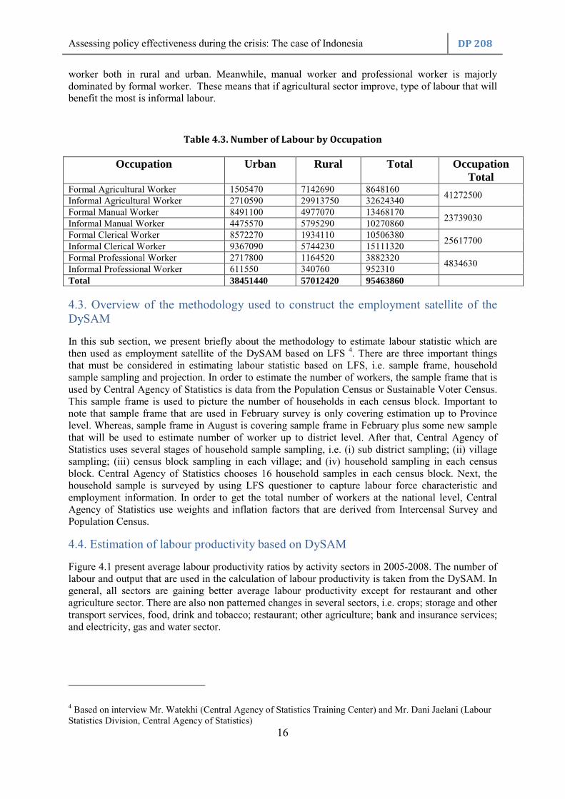
It is also interesting to analyze the labour statistic by occupation and location for both formal and informal sector. Table 4.3 shows that informality is majorly exist for agriculture worker and clerical
3 Based on interview Mr. Setyanto and Mrs. Nina Suri (Statistic of Account Division, Central Agency of Statistics)
Assessing policy effectiveness during the crisis: The case of Indonesia DP 208
16
worker both in rural and urban. Meanwhile, manual worker and professional worker is majorly dominated by formal worker. These means that if agricultural sector improve, type of labour that will benefit the most is informal labour.
Table 4.3. Number of Labour by Occupation
Occupation Urban Rural Total Occupation Total
Formal Agricultural Worker 1505470 7142690 8648160 41272500
Informal Agricultural Worker 2710590 29913750 32624340 Formal Manual Worker 8491100 4977070 13468170
23739030 Informal Manual Worker 4475570 5795290 10270860 Formal Clerical Worker 8572270 1934110 10506380
25617700 Informal Clerical Worker 9367090 5744230 15111320 Formal Professional Worker 2717800 1164520 3882320
4834630 Informal Professional Worker 611550 340760 952310 Total 38451440 57012420 95463860 4.3. Overview of the methodology used to construct the employment satellite of the DySAM
In this sub section, we present briefly about the methodology to estimate labour statistic which are then used as employment satellite of the DySAM based on LFS 4. There are three important things that must be considered in estimating labour statistic based on LFS, i.e. sample frame, household sample sampling and projection. In order to estimate the number of workers, the sample frame that is used by Central Agency of Statistics is data from the Population Census or Sustainable Voter Census. This sample frame is used to picture the number of households in each census block. Important to note that sample frame that are used in February survey is only covering estimation up to Province level. Whereas, sample frame in August is covering sample frame in February plus some new sample that will be used to estimate number of worker up to district level. After that, Central Agency of Statistics uses several stages of household sample sampling, i.e. (i) sub district sampling; (ii) village sampling; (iii) census block sampling in each village; and (iv) household sampling in each census block. Central Agency of Statistics chooses 16 household samples in each census block. Next, the household sample is surveyed by using LFS questioner to capture labour force characteristic and employment information. In order to get the total number of workers at the national level, Central Agency of Statistics use weights and inflation factors that are derived from Intercensal Survey and Population Census.
4.4. Estimation of labour productivity based on DySAM
Figure 4.1 present average labour productivity ratios by activity sectors in 2005-2008. The number of labour and output that are used in the calculation of labour productivity is taken from the DySAM. In general, all sectors are gaining better average labour productivity except for restaurant and other agriculture sector. There are also non patterned changes in several sectors, i.e. crops; storage and other transport services, food, drink and tobacco; restaurant; other agriculture; bank and insurance services; and electricity, gas and water sector.
4 Based on interview Mr. Watekhi (Central Agency of Statistics Training Center) and Mr. Dani Jaelani (Labour Statistics Division, Central Agency of Statistics)

Assessing policy effectiveness during the crisis: The case of Indonesia DP 208
17
Figure 4.1. Productivity by Economic Activity for 2005-2008
0 400000 800000 1200000
Crops
Other Agriculture
Livestock
Forestry
Fishery
Coal, Metal, Petroleum Mining
Mining and Quarry
Food, Beverages and Tobacco
Textile, Wearing apparel, Garment and
Leather
Wood
Paper, Print, Transp, Metal Product,
other industry
Chemical, Fertilizer, Clay and Cement
Electricity, Gas and Water
RoadLI
RoadKI
Irrigation
Construction
Trade Services
Restaurant
Hotel Affairs
Land Transportation Services
Air, Water Transportation and
Communication
Storage, Other Transportation Service
Bank, Insurance, and Services
Real Estate and Business Services
Government, Defensive, Education, and
Social Services
Other Individual and Household Services
2008
2007
2006
2005
Assessing policy effectiveness during the crisis: The case of Indonesia DP 208
18
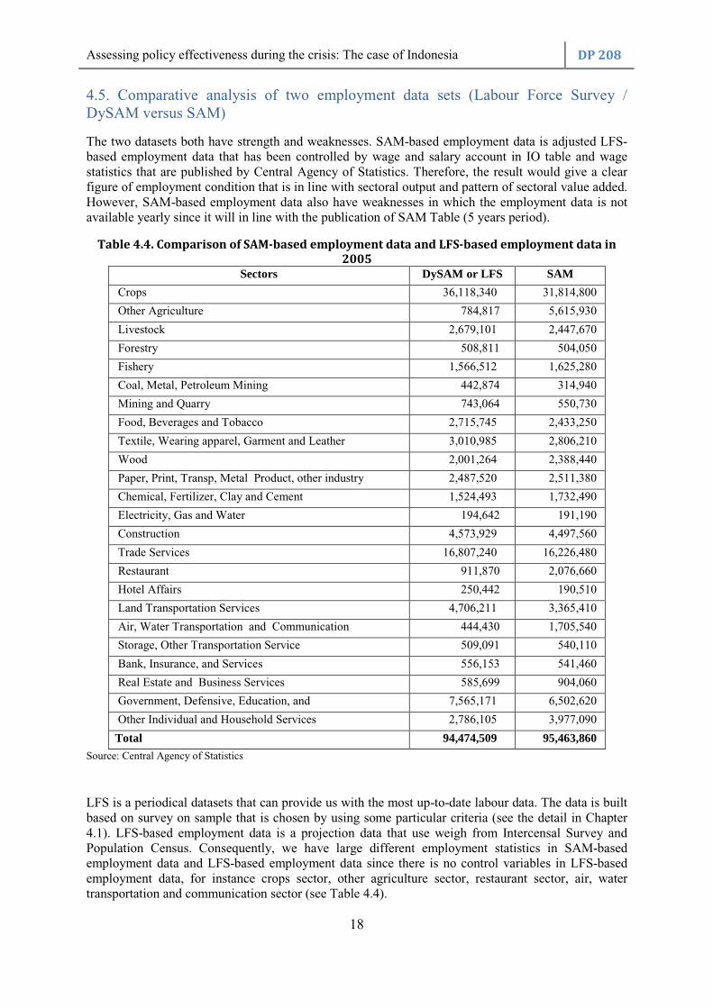
4.5. Comparative analysis of two employment data sets (Labour Force Survey / DySAM versus SAM)
The two datasets both have strength and weaknesses. SAM-based employment data is adjusted LFS-based employment data that has been controlled by wage and salary account in IO table and wage statistics that are published by Central Agency of Statistics. Therefore, the result would give a clear figure of employment condition that is in line with sectoral output and pattern of sectoral value added. However, SAM-based employment data also have weaknesses in which the employment data is not available yearly since it will in line with the publication of SAM Table (5 years period).
Table 4.4. Comparison of SAM-based employment data and LFS-based employment data in
2005
Sectors DySAM or LFS SAM
Crops 36,118,340 31,814,800
Other Agriculture 784,817 5,615,930
Livestock 2,679,101 2,447,670
Forestry 508,811 504,050
Fishery 1,566,512 1,625,280
Coal, Metal, Petroleum Mining 442,874 314,940
Mining and Quarry 743,064 550,730
Food, Beverages and Tobacco 2,715,745 2,433,250
Textile, Wearing apparel, Garment and Leather 3,010,985 2,806,210
Wood 2,001,264 2,388,440
Paper, Print, Transp, Metal Product, other industry 2,487,520 2,511,380
Chemical, Fertilizer, Clay and Cement 1,524,493 1,732,490
Electricity, Gas and Water 194,642 191,190
Construction 4,573,929 4,497,560
Trade Services 16,807,240 16,226,480
Restaurant 911,870 2,076,660
Hotel Affairs 250,442 190,510
Land Transportation Services 4,706,211 3,365,410
Air, Water Transportation and Communication 444,430 1,705,540
Storage, Other Transportation Service 509,091 540,110
Bank, Insurance, and Services 556,153 541,460
Real Estate and Business Services 585,699 904,060
Government, Defensive, Education, and 7,565,171 6,502,620
Other Individual and Household Services 2,786,105 3,977,090
Total 94,474,509 95,463,860
Source: Central Agency of Statistics
LFS is a periodical datasets that can provide us with the most up-to-date labour data. The data is built based on survey on sample that is chosen by using some particular criteria (see the detail in Chapter 4.1). LFS-based employment data is a projection data that use weigh from Intercensal Survey and Population Census. Consequently, we have large different employment statistics in SAM-based employment data and LFS-based employment data since there is no control variables in LFS-based employment data, for instance crops sector, other agriculture sector, restaurant sector, air, water transportation and communication sector (see Table 4.4).
Assessing policy effectiveness during the crisis: The case of Indonesia DP 208
19
4.6. Recommendations for estimation of employment for the DySAM employment satellite account
Based on Chapter 4.1, SAM-based employment data has been controlled by wage and salary account in IO Table and wage statistic. Therefore, employment data for DySAM employment satellite should be formulated by considering LFS data and then control by control variable which is done in SAM-based employment data. However, SAM-based employment data only available for particular year, the latest one is 2005. In this study we propose another approach to formulate DySAM employment satellite. This approach is the most feasible approach since wage and salary account in IO Table only available every 5 years. Moreover, this approach also makes corrections to the previous DySAM employment satellite, particularly on crops sector, other agriculture sector, and air, water transportation and communication sector.
This approach consists of three steps, hence:
1. Re-estimate employment statistics by sector based on LFS data and then calculate yearly growth of employment in each sector.
2. Calculate number of labour in 2006 up to 2008 by using employment statistic in SAM Table 2005 and growth of employment which is resulted in (a). Number of employment in 2005 must be exactly the same with employment statistic in SAM Table 2005.
3. Control total number of labor in (c) with total number of labor in LFS for each year and each sector. Total number of labours that are used in this approach is based on LFS data in August. Labour is defined as worker who are 10 years old and above.
4.7. New employment estimates derived for the DySAM employment satellite account for 2005 -2008
Based on steps that are taken in Chapter 4.5, we have new estimates of employment statistic which can be shown in Annex 5. The figure suggests that changes in the employment in each sector across years are not too fluctuated. Some sectors experienced increasing level of employment and some others had a negative trend of employment. The basic question that might arisen here is how much difference the result of new estimation with the one that generated by DySAM approach. Table 4.5 shows the comparison of the two datasets by looking the changes of employment in each year respect to number of labour in 2005. In general, the new estimation does not significantly change the employment dataset except for the other agriculture sector. In DySAM-based employment database, the definition of main industry in agriculture and other agriculture for 2005-2006 is different with the one for 2007-2008. Consequently, number of labour in other agriculture for 2007 increased substantially more than 17 times higher than number of labour in 2005. If we assume that the definition is unchanged, we should have employment statistic that is not significantly change across year except there is an economic shock. Table 4.5 shows that the new estimates of employment result a less fluctuated employment statistic particularly on other agriculture sector. Sector that has highest employment changes across years is restaurant sector as much as 3.9 per cent in 2007 relative to 2005.

Assessing policy effectiveness during the crisis: The case of Indonesia DP 208
20
Table 4.5. Changes of employment respect to 2005
Sectors DySAM estimation Revised estimation
2005 2006 2007 2008 2005 2006 2007 2008 Crops 1.000 0.964 0.584 0.560 1.000 0.964 0.963 0.960
Other Agriculture 1.000 0.356 17.960 18.753 1.000 0.803 0.630 0.615
Livestock 1.000 1.178 1.556 1.657 1.000 1.035 1.350 1.392
Forestry 1.000 1.231 1.219 1.327 1.000 1.207 1.161 1.261
Fishery 1.000 0.990 1.186 1.150 1.000 0.970 1.130 1.093
Coal, Metal, Petroleum Mining 1.000 1.035 1.098 1.215 1.000 1.103 1.141 1.253
Mining and Quarry 1.000 0.959 1.158 1.169 1.000 0.940 1.102 1.110
Food, Beverages and Tobacco 1.000 1.118 1.144 1.157 1.000 1.096 1.090 1.099 Textile, Wearing apparel, Garment and Leather
1.000 0.987 0.970 0.989 1.000 0.967 0.924 0.940
Wood 1.000 0.888 0.817 0.786 1.000 0.896 0.886 0.832 Paper, Print, Transp, Metal Product, other industry
1.000 0.940 1.116 1.127 1.000 0.922 1.063 1.070
Chemical, Fertilizer, Clay and Cement
1.000 1.042 1.126 1.207 1.000 1.021 1.072 1.147
Electricity, Gas and Water 1.000 1.171 0.899 1.034 1.000 1.148 0.856 0.982
RoadLI 1.000 1.059 1.177 1.245 1.000 1.038 1.121 1.183
RoadKI 1.000 0.958 1.136 1.102 1.000 0.939 1.082 1.046
Irrigation 1.000 1.011 1.156 1.137 1.000 0.991 1.101 1.080
Construction 1.000 1.021 1.100 1.164 1.000 1.001 1.048 1.106
Trade Services 1.000 1.039 0.992 1.030 1.000 1.019 0.944 0.978
Restaurant 1.000 1.711 4.110 4.136 1.000 1.677 3.914 3.929
Hotel Affairs 1.000 1.134 1.226 1.312 1.000 1.112 1.168 1.246
Land Transportation Services 1.000 0.966 0.939 0.953 1.000 0.948 0.895 0.905 Air, Water Transportation and Communication
1.000 1.090 1.321 1.645 1.000 1.065 1.255 1.567
Storage, Other Transportation Service
1.000 1.258 1.888 1.906 1.000 1.230 1.798 1.811
Bank, Insurance, and Services 1.000 1.220 1.331 1.243 1.000 1.195 1.268 1.181
Real Estate and Business Services 1.000 1.140 1.129 1.314 1.000 1.117 1.075 1.248 Government, Defensive, Education, and
1.000 1.176 1.334 1.425 1.000 1.083 1.090 1.056
Other Individual and Household Services
1.000 0.894 0.712 0.848 1.000 1.071 1.145 1.459
Source: Author’s own analysis

Assessing policy effectiveness during the crisis: The case of Indonesia DP 208
21
4.8. New labour productivity estimates for 2005 -2008
Figure 4.2 shows the new labour productivity based on new estimates of employment statistics which is mentioned in Chapter 4.6 and Annex 6. Generally, productivity statistics in each sector based on new estimation are quite similar with the DySAM-based productivity statistics in Chapter 4.3 except for particular sectors. If we compare Figure 4.1 and Figure 4.2, some sectors such as other individual and household services sector, air, water transportation and communication sector, real estate and business services sector, restaurant sector and other agriculture sector in the new labour productivity estimates have lower productivity relative to the DySAM-based productivity statistics. Meanwhile, productivity of coal, metal, petroleum mining sector in the new estimates is higher than the DySAM-based productivity statistics.
In terms of pattern of productivity changes, in the new estimates we also found that almost all sectors experienced a relatively higher productivity across years. However there are also non patterned-changes such as the productivity changes in real estate and business services sector, bank, insurance and services sectors, etc. If we compare Figure 4.1 and Figure 4.2, we found that pattern in the productivity changes for several sectors differ between the two datasets, for instance in electricity, gas and water sector and coal, metal, petroleum mining sector.

Assessing policy effectiveness during the crisis: The case of Indonesia DP 208
22
Figure 4.2. A New Estimates of Productivity by Economic Activity for 2005-2008
0 400000 800000 1200000 1600000
Crops
Other Agriculture
Livestock
Forestry
Fishery
Coal, Metal, Petroleum Mining
Mining and Quarry
Food, Beverages and Tobacco
Textile, Wearing apparel, Garment and
Leather
Wood
Paper, Print, Transp, Metal Product,
other industry
Chemical, Fertilizer, Clay and Cement
Electricity, Gas and Water
RoadLI
RoadKI
Irrigation
Construction
Trade Services
Restaurant
Hotel Affairs
Land Transportation Services
Air, Water Transportation and
Communication
Storage, Other Transportation Service
Bank, Insurance, and Services
Real Estate and Business Services
Government, Defensive, Education, and
Social Services
Other Individual and Household Services
2008
2007
2006
2005

Assessing policy effectiveness during the crisis: The case of Indonesia DP 208
23
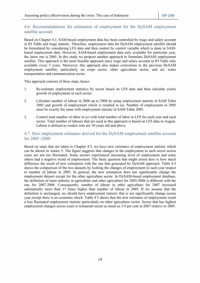
Chapter 5: Simulation and results 5.1. Data on the realization rates of the fiscal stimulus
The total realization rate of the fiscal stimulus was 83.84 per cent or equal to 61.4 trillion IDR. Based on its objective, the realization of fiscal stimulus consists of 78.7 per cent realization of the first group of programs, 85 per cent realization of second group of programs, and 91.4 per cent realization of third group of programs (See the detail on Table 5.1).
The realization of fiscal stimulus in the first group of fiscal stimulus instruments, hence to maintain and improve people purchasing power was the lowest relative to others. These are largely contributed by the very low realization rates on value added tax cut along with personal income tax cut which amounted 61.35 per cent and 79.70 per cent respectively.
In the second group of fiscal stimulus instruments, three instruments have 100 per cent and nearly 100 per cent realization rate, namely corporate income tax cut, government capital expenditure to State Owned Enterprises, and subsidy. The other 3 instruments have relatively low realization rates, especially on tariff import tax cut, which was only less than half per cent. The poor realization of these instruments was due to a relatively late implementation date. The instrument was only effective in the second semester 2009, which is late, especially as firms usually sign contracts on raw material buying in the beginning of the year. Moreover, it is also affected by the lower demand of imported raw material due to lower global demand associated with the crisis.
The highest realization rate was in the third group of program, increase investment in labour intensive infrastructure. The realization rate achieved was 91.4 per cent of the target. Almost all instruments achieved nearly 100 per cent realization except for government investment for employment program that only achieved 84.43 per cent and government investment for agricultural infrastructure that has zero realization rates. Generally, factors that became barriers in the infrastructure program implementation were lack of supporting regulation, complicated administration and accounting process, tender process, and implementation process. Beside of these factors, thrift also become another determinant, for instance in the tender process. The particular problems of each infrastructure component of the fiscal stimulus include:
1. Fiscal stimulus on transportation infrastructure: the problem occurred due to incomplete administration requirements for fund disbursement (Konawe Port), unfinished process in the provision of land (Kuala Semboja Port) and natural disaster, such as earth quake (Carocok Padang Port).
2. Fiscal stimulus on housing infrastructure: The problem arose due to Contract Change Order (CCO) in some projects and the provision of land. The consequence of CCO is non-optimal utilization of the property.
3. Fiscal stimulus on employment infrastructure: the problem occurred due to incomplete administration requirements for fund disbursement.
4. Fiscal stimulus on market infrastructure: the problem occurred due to incomplete administration requirements for fund disbursement, land provision, tender process and implementation process.
Assessing policy effectiveness during the crisis: The case of Indonesia DP 208
24
Table 5.1. Realization of the Fiscal Stimulus
Source: Ministry of Finance
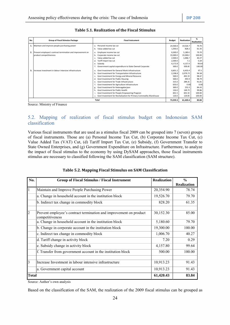
5.2. Mapping of realization of fiscal stimulus budget on Indonesian SAM classification
Various fiscal instruments that are used as a stimulus fiscal 2009 can be grouped into 7 (seven) groups of fiscal instruments. Those are (a) Personal Income Tax Cut, (b) Corporate Income Tax Cut, (c) Value Added Tax (VAT) Cut, (d) Tariff Import Tax Cut, (e) Subsidy, (f) Government Transfer to State Owned Enterprises, and (g) Government Expenditure on Infrastructure. Furthermore, to analyze the impact of fiscal stimulus to the economy by using DySAM approaches, those fiscal instruments stimulus are necessary to classified following the SAM classification (SAM structure).
Table 5.2. Mapping Fiscal Stimulus on SAM Classification
No. Group of Fiscal Stimulus / Fiscal Instrument Realization % Realization
1 Maintain and Improve People Purchasing Power 20,354.90 78.74
a. Change in household account in the institution block 19,526.70 79.70
b. Indirect tax change in commodity block 828.20 61.35
2 Prevent employee’s contract termination and improvement on product
competitiveness 30,152.30 85.00
a. Change in household account in the institution block 5,180.60 79.70
b. Change in corporate account in the institution block 19,300.00 100.00
c. Indirect tax change in commodity block 1,006.70 40.27
d. Tariff change in activity block 7.20 0.29
e. Subsidy change in activity block 4,157.80 99.64
f. Transfer from government account in the institution block 500.00 100.00
3 Increase Investment in labour intensive infrastructure 10,913.23 91.43
a. Government capital account 10,913.23 91.43
Total 61,420.43 83.84
Source: Author’s own analysis
Based on the classification of the SAM, the realization of the 2009 fiscal stimulus can be grouped as
No. Group of Fiscal Stimulus Package Fiscal Instrument Budget Realization%
Realization
1. Maintain and improve people purchasing power a. Personel Income tax cut 24,500.0 19,526.7 79.70
b. Value added tax cut 1,350.0 828.2 61.35
2. a. Employee income tax cut 6,500.0 5,180.6 79.70
b. Corporate income tax cut 19,300.0 19,300.0 100.00
c. Value added tax cut 2,500.0 1,006.7 40.27
d. Tariff Import tax cut 2,500.0 7.2 0.29
e. Subsidy 4,172.8 4,157.8 99.64
f. Government capital expenditure to State Owned Corporate 500.0 500.00 100.00
3. Increase investment in labour intensive infrastructure a. Govt Investment for General Work Infrastructure 6,601.2 6,433.4 97.5
b. Govt Investment for Transportation Infrastructure 2,198.8 2,079.73 94.58
c. Govt Investment for Energy and Mineral Resource 500.0 492.35 98.47
d. Govt Investment for Public Housing 500.0 493.9 98.79
e. Govt Investment for Trade Infrastructure 315.0 289.20 91.81
f. Govt Investment for Agriculture Infrastructure 650.0 0.00 0.00
g. Govt Investment for Ketenagakerjaan 300.0 253.3 84.43
h. Govt Investment for Public Health 150.0 149.79 99.86
i. Govt Investment for People Empowering Program 601.5 601.50 100.00
j. Govt Investment for Revitalization for Primary Commodity Warehouse 120.0 120.00 100.00
73,259.3 61,420.4 83.84 Total
Prevent employee's contract termination and improvement on
product competitiveness
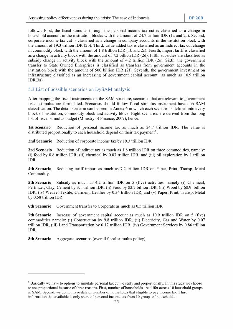
Assessing policy effectiveness during the crisis: The case of Indonesia DP 208
25
follows. First, the fiscal stimulus through the personal income tax cut is classified as a change in household account in the institution blocks with the amount of 24.7 trillion IDR (1a and 2a). Second, corporate income tax cut is classified as a change in company accounts in the institution block with the amount of 19.3 trillion IDR (2b). Third, value added tax is classified as an Indirect tax cut change in commodity block with the amount of 1.8 trillion IDR (1b and 2c). Fourth, import tariff is classified as a change in activity block with the amount of 7.2 billion IDR (2d). Fifth, subsidies are classified as subsidy change in activity block with the amount of 4.2 trillion IDR (2e). Sixth, the government transfer to State Owned Enterprises is classified as transfers from government accounts in the institution block with the amount of 500 billion IDR (2f). Seventh, the government investment on infrastructure classified as an increasing of government capital account as much as 10.9 trillion IDR(3a).
5.3 List of possible scenarios on DySAM analysis
After mapping the fiscal instruments on the SAM structure, scenarios that are relevant to government fiscal stimulus are formulated. Scenarios should follow fiscal stimulus instrument based on SAM classification. The detail scenario can be seen in Annex 6 in which each scenario is defined into every block of institution, commodity block and activity block. Eight scenarios are derived from the long list of fiscal stimulus budget (Ministry of Finance, 2009), hence:
1st Scenario Reduction of personal income tax as much as 24.7 trillion IDR. The value is distributed proportionally to each household depend on their tax payment5 .
2nd Scenario Reduction of corporate income tax by 19.3 trillion IDR.
3rd Scenario Reduction of indirect tax as much as 1.8 trillion IDR on three commodities, namely: (i) food by 0.8 trillion IDR; (ii) chemical by 0.03 trillion IDR; and (iii) oil exploration by 1 trillion IDR.
4th Scenario Reducing tariff import as much as 7.2 trillion IDR on Paper, Print, Transp, Metal Commodity.
5th Scenario Subsidy as much as 4.2 trillion IDR on 5 (five) activities, namely (i) Chemical, Fertilizer, Clay, Cement by 3.1 trillion IDR, (ii) Food by 82.7 billion IDR, (iii) Wood by 68.9 billion IDR, (iv) Weave, Textile, Garment, Leather by 0.34 trillion IDR, and (v) Paper, Print, Transp, Metal by 0.58 trillion IDR.
6th Scenario Government transfer to Corporate as much as 0.5 trillion IDR
7th Scenario Increase of government capital account as much as 10.9 trillion IDR on 5 (five) commodities namely: (i) Construction by 9.8 trillion IDR, (ii) Electricity, Gas and Water by 0.07 trillion IDR, (iii) Land Transportation by 0.17 trillion IDR, (iv) Government Services by 0.86 trillion IDR.
8th Scenario Aggregate scenarios (overall fiscal stimulus policy).
5 Basically we have to options to simulate personal tax cut, -evenly and proportionally. In this study we choose to use proportional because of three reasons. First, number of households are differ across 10 household groups in SAM. Second, we do not have data on number of households that eligible to pay income tax. Third, information that available is only share of personal income tax from 10 groups of households.

Assessing policy effectiveness during the crisis: The case of Indonesia DP 208
26
5.4. The impact of fiscal stimulus on Indonesian economic performance 5.4.1. Output and employment by sector
In this sub chapter we present the character of sector based on its output and employment. Table 5.3 show the contribution of each sector on national output and employment. In general, manufacturing sectors have relatively larger contribution on national output but lower contribution on employment. Oppositely, agriculture sector has relatively smaller contribution on national output and larger contribution on employment. Only trade sector that has relatively high contribution on both national output and employment.
Table 5.3. Contribution of Sector on National Economy in terms of Output and Employment
Sector Output Employment Crops 4% 29% Other Agriculture 2% 3% Livestock 1% 3% Forestry 0% 1% Fishery 1% 2% Coal, Metal, Petroleum Mining 6% 0% Mining and Quarry 1% 1% Food, Beverages and Tobacco 9% 3% Textile, Wearing apparel, Garment and Leather 4% 3% Wood 2% 2% Paper, Print, Transp, Metal Product, other industry 12% 2% Chemical, Fertilizer, Clay and Cement 11% 2% Electricity, Gas and Water 2% 0% RoadLI 1% 2% RoadKI 3% 1% Irrigation 4% 0% Construction 2% 1% Trade Services 9% 15% Restaurant 3% 8% Hotel Affairs 1% 0% Land Transportation Services 3% 3% Air, Water Transportation and Communication 4% 5% Storage, Other Transportation Service 1% 1% Bank, Insurance, and Services 3% 1% Real Estate and Business Services 3% 1% Government, Defensive, Education, and 5% 7% Other Individual and Household Services 3% 5%
Source: Central Agency of Statistics
5.4.2. The impact of each fiscal stimulus instrument on production
activities
The impact of each fiscal stimulus instrument across the eight scenarios for production activities is presented in this section. In general, all fiscal stimulus instruments will have positive impact on production activities. Before analyzing the impact for each fiscal instrument, it is really important to consider the magnitude of stimulus on each scenario. Scenario 8 is the accumulation of all 7 scenarios, thus the size of the shocks is the largest among others. Consequently, we can easily predict that the impact of scenario 8 will be largest relative to others.

Assessing policy effectiveness during the crisis: The case of Indonesia DP 208
27
Table 5.4. The Impact of Each Fiscal Stimulus Instrument on Production Activities
No Production Sector
Baseline
Condition Scen 1 Scen 2 Scen 3 Scen 4 Scen 5 Scen 6 Scen 7 Scen 8
(Billion IDR)
1 Crops
391.378,88
3.824,04
142,63
294.35
0,56
305,79 3,70
927.15
5,498.21
(%)
0,98
0,04
0.08
0,00
0,08 0,00
0.24
1.40
2 Other Agriculture
168.016,69
1.097,96
40,86
112.90
0,28
215,55 1,06
328.53
1,797.14
(%)
0,65
0,02
0.07
0,00
0,13 0,00
0.20
1.07
3 Livestock
118.102,58
1.227,65
45,72
76.76
0,18
96,96 1,18
298.70
1,747.15
(%)
1,04
0,04
0.06
0,00
0,08 0,00
0.25
1.48
4 Forestry and Hunting
45.260,31
98,97
3,72
4.37
0,02
20,51 0,10
225.82
353.50
(%)
0,22
0,01
0.01
0,00
0,05 0,00
0.50
0.78
5 Fishery
126.245,42
1.276,57
47,61
71.08
0,18
97,66 1,23
302.50
1,796.83
(%)
1,01
0,04
0.06
0,00
0,08 0,00
0.24
1.42
6 Coal, Metal, Petroleum Mining
596.095,05
839,34
31,12
1,046.90
0,28
585,91 0,81
527.13
3,031.49
(%)
0,14
0,01
0.18
0,00
0,10 0,00
0.09
0.51
7 MiningQuarry
59.264,29
38,44
1,42
2.41
0,01
19,76 0,04
528.37
590.46
(%)
0,06
0,00
0.00
0,00
0,03 0,00
0.89
1.00
8 Food, Drink and Tobacco
906.172,49
8.220,48
305,52
1,105.20
1,29
719,94 7,91
1,968.37
12,328.70
(%)
0,91
0,03
0.12
0,00
0,08 0,00
0.22
1.36
9 Weave, Textile, Garment and Leather
398.260,03
1.628,84
61,17
59.07
9,84
606,15 1,58
410.41
2,777.07
(%)
0,41
0,02
0.01
0,00
0,15 0,00
0.10
0.70
10 Wood
146.035,76
252,55
9,38
9.58
0,04
103,48 0,24
455.11
830.39
(%)
0,17
0,01
0.01
0,00
0,07 0,00
0.31
0.57
11
Paper, Print, Transp, Metal
Product
1.199.138,72
4.395,83
163,18
182.30
0,83
1.079,57 4,23
2,544.43
8,370.37
(%)
0,37
0,01
0.02
0,00
0,09 0,00
0.21
0.70
12
Chemical, Fertilizer, Clay and
Cement
1.068.163,96
3.484,34
129,10
199.94
1,18
3.664,37 3,34
2,520.70
10,002.97
(%)
0,33
0,01
0.02
0,00
0,34 0,00
0.24
0.94
13 Electricity, Gas and Water
165.049,14
1.063,57
39,47
43.53
0,45
142,07 1,02
415.02
1,705.14
(%)
0,64
0,02
0.03
0,00
0,09 0,00
0.25
1.03
14 RoadLI
129.764,66
29,48
1,08
1.95
0,01
3,84 0,03
1,303.43
1,339.82
(%)
0,02
0,00
0.00
0,00
0,00 0,00
1.00
1.03
15 RoadKI
297.437,90
67,57
2,48
4.47
0,02
8,80 0,06
2,987.64
3,071.05
(%)
0,02
0,00
0.00
0,00
0,00 0,00
1.00
1.03
16 Irrigation
373.375,02
84,82
3,12
5.61
0,02
11,04 0,08
3,750.39
3,855.10
(%)
0,02
0,00
0.00
0,00
0,00 0,00
1.00
1.03
17 Construction
156.119,93
35,47
1,30
2.35
0,01
4,62 0,03
1,568.16
1,611.94
(%)
0,02
0,00
0.00
0,00
0,00 0,00
1.00
1.03
18 Trade Services
864.285,82
5.212,98
186,84
239.09
1,23
550,05 4,84
2,183.26
8,378.29
(%)
0,60
0,02
0.03
0,00
0,06 0,00
0.25
0.97
19 Restaurant
329.990,27
3.050,96
114,36
107.46
0,47
241,10 2,96
807.34
4,324.66
Assessing policy effectiveness during the crisis: The case of Indonesia DP 208
28
(%)
0,92
0,03
0.03
0,00
0,07 0,00
0.24
1.31
20 Hotel Affairs
49.318,21
167,07
6,16
6.33
0,03
15,12 0,16
54.34
249.22
(%)
0,34
0,01
0.01
0,00
0,03 0,00
0.11
0.51
21 Land Transportation Service
274.825,49
1.851,16
68,26
83.02
0,43
191,82 1,77
834.43
3,030.90
(%)
0,67
0,02
0.03
0,00
0,07 0,00
0.30
1.10
22
Air, WaterTransportation and
Communication
349.882,67
2.226,71
83,00
91.99
0,43
211,80 2,15
730.03
3,346.12
(%)
0,64
0,02
0.03
0,00
0,06 0,00
0.21
0.96
23 Storage, Other Tranportation Service
66.629,08
345,14
12,72
15.51
0,09
37,53 0,33
128.22
539.55
(%)
0,52
0,02
0.02
0,00
0,06 0,00
0.19
0.81
24 Bank, Insurance, and Services
301.273,72
2.217,84
82,52
103.34
0,57
241,60 2,14
793.03
3,441.03
(%)
0,74
0,03
0.03
0,00
0,08 0,00
0.26
1.14
25 Real Estate and Business Services
302.316,35
2.009,86
74,26
83.16
0,42
197,23 1,92
880.57
3,247.43
(%)
0,66
0,02
0.03
0,00
0,07 0,00
0.29
1.07
26
Government, Defensive, Educaion,
and Other Social Services
517.755,08
2.622,13
97,67
96.03
0,39
208,65 2,53
1,519.97
4,547.38
(%)
0,51
0,02
0.02
0,00
0,04 0,00
0.29
0.88
27 Other Individu and Household Services
287.679,68
2.069,27
76,69
86.83
0,37
189,10 1,99
646.37
3,070.63
(%)
0,72
0,03
0.03
0,00
0,07 0,00
0.22
1.07
Total 9.687.837,22
49.439,03
1.831,39
4,135.57
19,62
9.770,02 47,45
29,639.45
94,882.52
Note: Baseline is the condition without fiscal stimulus injection Source: Author’s own analysis
Personal income tax reduction (scenario 1) will have larger impact on production activities in almost all sectors, except for the infrastructure sectors, such as labour and capital intensive roads, irrigation and the rest of the construction sector. It is important to note here that the total budget that are spent through this scenario is substantial - as much as 24.7 trillion IDR. According to the results of the simulations, the five sectors that will experience the highest impact are livestock, fishery, crops, restaurant and food, drink and tobacco sectors. Personal income tax reduction will increase disposable income and then lead to an increase in the purchasing power. Since Indonesian people spend a larger proportion on food products, the higher disposable income should result in higher consumption of food commodities.
Scenario 2 and scenario 6 are very similar. In both scenarios enterprises are the main concern. The differences between the two scenarios are the magnitude of the shocks and type of instrument that are used in each scenario. In scenario 2, the government uses a tax instrument, whereas in scenario 6 the government uses a transfer instrument. Consequently, the impact on production activities is nearly the same in both scenarios, except for the size of the impact. Generally, a corporate income tax reduction will cause both direct and indirect impact. A corporate income tax directly will increase corporate investment and indirectly will increase final demand of goods and services through an increase on institution transfer from corporate to government and household. The highest impact is expected to existed in crops sector, livestock sector, fishery sector, food, drink and tobacco sector, restaurant sector, bank, insurance and services sector and other individual and household services sector.
Another instrument that can be used by government is value-added tax (VAT). A VAT reduction (scenario 3) on the food sector will not only have an impact on the food sector, but also on agricultural sectors except for forestry sector. Higher activities in the food sector will cause higher demand on input for the food sector. Therefore, the production activities of the agricultural sectors, such as crops, other crops, livestock, and fishery sector will increase as well. Based on this scenario, we can see that the magnitude of the fiscal stimulus matters, since the impacts are relatively larger in

Assessing policy effectiveness during the crisis: The case of Indonesia DP 208
29
the coal, metal, petroleum mining sector and food sector. In other hand, it will only has slightly increase the production activities of chemical industry, since the budget is only 0.03 trillion IDR. This is also the case for scenario 4, in which tariff import reduction in other industry sectors is approximately 0.007 trillion IDR. Such an investment will have a very small impact on the sector approximately less than 0.01 per cent.
In scenario 5, a subsidy on a particular sector will only have a moderate impact on the chemical sector and the textile sector and other agriculture. Moreover, it will only have a small impact on food sector and paper, print and other industry sector. In scenario 7, the government invested more on infrastructure. As expected, the impact on the production activities in all sector are quite significant, especially on road sector, irrigation sector, construction sector and electricity, gas and water sector. Higher activities in the construction sector increases the demand for raw materials, therefore, the scenario sees an also increase the production activities of the mining and query sector.
In the last scenario (Scenario 8), the highest impact of all fiscal stimulus policy is expected to exist in agricultural sector and agriculture-related industry –food, drink and tobacco sector-. If we aggregate the sector, fiscal stimulus policy is expected will increase the output of manufacturing sector, construction sector and trade sector by 0.9 per cent, 1.03 per cent, and 1.04 per cent respectively. These impact are still smaller than the impact of financial crisis 2008 on those three sector in the fourth quartile 2008 (see Annex 1).
To sum up, agricultural sector seems to benefit moderately from any scenario and even received the highest impact if the fiscal stimulus policy is conducted through personal tax cut and corporate income tax cut. Manufacturing sector is expected to experienced highest impact if subsidy on activities is implemented. Interestingly, the impact of value added tax cut on manufacturing sector performance is expected not too significant in magnitude. The argument is mainly due to the size of the shock which is only 1.8 trillion IDR and mostly (about 1 trillion IDR) was distributed on Coal, Metal Petroleum Mining sector. Meanwhile, construction sector, road sector and irrigation sector is only benefit from fiscal stimulus policy on infrastructure. Due to the financial crisis 2008, sectors that are affected the most are construction sector, trade sector and manufacturing sector (Central Bank of Indonesia, 2009). Therefore, mix policies between subsidy and fiscal stimulus policy on infrastructure are types of fiscal instrument that are relevant to stimulate the sectors that are experiencing a decline due to financial crisis 2008.
5.4.3. The impact of each fiscal stimulus instrument on labour income
In terms of labour income, the impacts are strongly related with the impact on production activities, since production activity is a function of production factors. Table 5.5 suggests that personal income tax reduction will have larger impact on agricultural workers, both formal and informal in urban and rural areas. Higher production activities in the agricultural sector will result in higher demand for labour. As a result, the type of labour that will get a higher percentage change on income are those who work in the agricultural sector. Interestingly, other types of workers also experienced a large positive impact, with percentages changes between 0.37 per cent up to 0.64 per cent. These results are all rational, since personal income tax reduction also will generate higher production activities in almost all services sectors. Therefore, it will trigger higher income for all types of workers including manual, clerical and professional worker.
Corporate tax reduction (Scenario 2) and subsidy (Scenario 5) are expected to increase labour income in all types of labour with the largest impact existed on agricultural worker both formal and informal in urban and rural areas. These are completely in line with the impact on production activities in which agricultural sector are expected to increase relatively higher than others. Scenarios 4 and 6 have a relatively small impact on labour income. Even though percentage changes in Table 5.4 are zero, there are some small changes that amount to less than 0.01 per cent.
In the third scenario, VAT reduction on particular sectors is expected to increase labour income at least 0.06 per cent for all agricultural worker both informal and formal in both urban and rural. This is
Assessing policy effectiveness during the crisis: The case of Indonesia DP 208
30
mainly due to the positive impact on activities in the agricultural sectors, except for forestry and hunting. The positive growth of production activities in almost all agricultural sub-sectors is mainly contributed by the improvement of food industry performance. The second highest impact will be accepted by rural and urban formal manual workers. This is mainly due to the impressive positive impact on production activities in the coal, metal and petroleum mining sector and food drinking and tobacco (food) sector. Even though the impact of VAT reduction is substantially large for the coal, metal and petroleum mining sector and food sector, these two sectors are more capital intensive. Therefore, the impact on labour will be moderate, particularly on manual worker since the share of manual formal worker on the sectors’ labour structure is relatively higher.
Fiscal stimulus on infrastructure (Scenario 7) is expected to increase labour income for all types of labour ranging between 0.23 up to 0.42 per cent. Formal manual worker in rural areas are expected to receive the highest impact. This type of workers is largely employed in the construction process. Since construction, road, and irrigation sector are mostly affected by infrastructure stimulus, therefore the results are completely rational. In scenario 8, all fiscal stimulus policy is expected to result highest impact on all agricultural worker both informal and formal in both urban and rural. Moreover, the impact on other types of workers are also significant with an increase at least 0.89 per cent.
In conclusion, agricultural worker is expected to gain a relatively high positive impact under any scenario except fiscal stimulus policy on infrastructure (scenario 7). If government focus on stimulating manufacturing sector performance, manual worker will benefit the most and the impact will be quite evenly distributed across types of worker ranging between 0.05 per cent to 0.11 per cent. Similar condition also existed if fiscal stimulus policy is implemented through an increase of government investment on infrastructure.

Assessing policy effectiveness during the crisis: The case of Indonesia DP 208
31
Table 5.5. The Impact of Each Fiscal Stimulus Instrument on Labor Income
No. Labor Classification
Baseline
Condition Scen 1
Scen
2
Scen
3
Scen
4 Scen 5
Scen
6 Scen 7 Scen 8
(Billion Rp)
1
Formal Agricultural Worker -
Rural
106.314,06
930,93
34,70
70.94
0,16
96,64
0,90
254.14
1,388.40
(%)
0,88
0,03
0.07
0,00
0,09
0,00
0.24
1.31
2
Formal Agricultural Worker -
Urban
26.387,63
233,34
8,70
16.65
0,04
22,86
0,23
65.40
347.20
(%)
0,88
0,03
0.06
0,00
0,09
0,00
0.25
1.32
3
Informal Agricultural Worker -
Rural
328.007,35
3.009,53
112,21
233.04
0,47
282,56
2,91
773.46
4,414.18
(%)
0,92
0,03
0.07
0,00
0,09
0,00
0.24
1.35
4 Informal Agricultural Worker - Urban
32.130,10
300,94
11,22
22.09
0,05
26,37
0,29
77.84
438.79
(%)
0,94
0,03
0.07
0,00
0,08
0,00
0.24
1.37
5 Formal Manual Worker - Rural
185.177,41
682,56
25,30
66.85
0,35
180,07
0,66
829.28
1,785.07
(%)
0,37
0,01
0.04
0,00
0,10
0,00
0.45
0.96
6 Formal Manual Worker - Urban
385.275,45
1.588,32
58,84
136.98
1,02
428,38
1,52
1,340.06
3,555.12
(%)
0,41
0,02
0.04
0,00
0,11
0,00
0.35
0.92
7 Informal Manual Worker - Rural
137.773,20
589,49
21,86
40.74
0,27
157,68
0,57
511.06
1,321.67
(%)
0,43
0,02
0.03
0,00
0,11
0,00
0.37
0.96
8
Informal Manual Worker -
Urban
112.072,33
510,41
18,90
33.80
0,24
89,39
0,49
457.20
1,110.44
(%)
0,46
0,02
0.03
0,00
0,08
0,00
0.41
0.99
9 Formal Clerical Worker - Rural
85.650,98
517,29
19,08
31.61
0,12
64,42
0,49
218.28
851.29
(%)
0,60
0,02
0.04
0,00
0,08
0,00
0.25
0.99
10 Formal Clerical Worker - Urban
458.527,77
2.695,97
99,46
149.69
0,70
364,21
2,58
1,186.88
4,499.48
(%)
0,59
0,02
0.03
0,00
0,08
0,00
0.26
0.98
11 Informal Clerical Worker - Rural
139.758,36
886,00
32,06
39.75
0,20
93,20
0,83
358.21
1,410.25
(%)
0,63
0,02
0.03
0,00
0,07
0,00
0.26
1.01
12
Informal Clerical Worker -
Urban
248.147,08
1.580,39
57,30
70.37
0,35
159,40
1,48
642.88
2,512.18
(%)
0,64
0,02
0.03
0,00
0,06
0,00
0.26
1.01
13
Formal Professional Worker -
Rural
66.735,18
337,56
12,55
16.32
0,06
34,01
0,33
195.22
596.04
(%)
0,51
0,02
0.02
0,00
0,05
0,00
0.29
0.89
14 Formal Professional Worker - Urban
200.276,73
983,40
36,48
56.57
0,21
131,63
0,94
627.74
1,836.97
(%)
0,49
0,02
0.03
0,00
0,07
0,00
0.31
0.92
15 Informal Professional Worker - Rural
12.694,24
57,04
2,10
3.00
0,01
9,33
0,05
53.06
124.60
(%)
0,45
0,02
0.02
0,00
0,07
0,00
0.42
0.98
16 Informal Professional Worker - Urban
30.775,27
136,66
5,06
6.02
0,03
20,93
0,13
115.84
284.68
(%)
0,44
0,02
0.02
0,00
0,07
0,00
0.38
0.93
Total
2.555.703,14
15.039,82
555,82
994.40
4,27
2.161,08
14,40
7,706.57
26,476.36
Source: Author’s own analysis

Assessing policy effectiveness during the crisis: The case of Indonesia DP 208
32
5.4.4. The impact of each fiscal stimulus instrument on household income
Generally, the impact of all instruments are positive on household income. All types of household will get higher income due to personal income tax cut policy. It is expected that household income to increase more than 0.9 per cent relative to the baseline. Groups of household that will benefit the most are the high income household both in urban and rural. Oppositely, agricultural employee will received the lowest impact due to personal tax cut policy. These results is mainly derived from the size of the injection which are relatively larger on those two groups of households.
Table 5.6. The Impact of Each Fiscal Stimulus Instrument on Household Income
No. Household
Classification
Baseline
Condition Scen 1 Scen 2 Scen 3
Scen
4 Scen 5
Scen
6 Scen 7 Scen 8
(Billion Rp)
1 Agriculture Employee
254.677,00
2,410.60
83.96
79.41
0.27
146.59
2.18
448.05
3,171.06
(%)
0.95
0.03
0.03
0.00
0.06
0.00
0.18
1.25
2 Small Farmer
368.451,27
3,867.95
135.05
154.83
0.48
267.75
3.50
799.06
5,228.60
(%)
1.05
0.04
0.04
0.00
0.07
0.00
0.22
1.42
3 Medium Farmer
200.526,91
2,081.64
89.44
90.28
0.32
172.52
2.32
521.29
2,957.82
(%)
1.04
0.04
0.05
0.00
0.09
0.00
0.26
1.48
4 Larger Farmer
195.230,87
2,271.51
113.86
98.64
0.30
181.04
2.95
505.53
3,173.83
(%)
1.16
0.06
0.05
0.00
0.09
0.00
0.26
1.63
5 Rural Non-Labour
519.167,29
4,968.23
205.87
191.32
0.76
418.69
5.33
1,449.20
7,239.40
(%)
0.96
0.04
0.04
0.00
0.08
0.00
0.28
1.39
6 Rural Low Income
176.303,51
1,730.03
62.13
74.37
0.25
148.49
1.61
452.87
2,469.76
(%)
0.98
0.04
0.04
0.00
0.08
0.00
0.26
1.40
7 Rural High Income
439.458,95
5,959.84
211.31
202.55
0.67
396.80
5.47
1,176.90
7,953.55
(%)
1.36
0.05
0.05
0.00
0.09
0.00
0.27
1.81
8 Urban Non Labor
704.260,06
7,438.21
241.98
241.14
1.28
610.29
6.27
1,936.27
10,475.44
(%)
1.06
0.03
0.03
0.00
0.09
0.00
0.27
1.49
9 Urban Low Income
248.718,81
3,080.23
118.90
89.09
0.42
212.78
3.08
651.35
4,155.86
(%)
1.24
0.05
0.04
0.00
0.09
0.00
0.26
1.67
10 Urban High
776.700,03
10,156.02
374.97
285.95
1.18
641.67
9.71
2,149.76
13,619.26
(%)
1.31
0.05
0.04
0.00
0.08
0.00
0.28
1.75
Total
3.883.494,70
43.964,26
1.637,48
1,507.58
5,93
3.196,61
42,42
10,090.29
60,444.57
Source: Author’s own analysis
Similar with previous findings, the impact of corporate tax cut (scenario 2) on household income is expected to increase income in all types of households with highest impact on larger farmer as much as 0.06 per cent. Similar figures can also be found in the Scenario 5 with the exception on urban non labour and urban low income. If government give subsidy to manufacturing sector, urban non labour and urban low income household will also received the highest benefit. The increase in subsidy is expected to result higher household income for all groups of households, ranging between 0.06 per cent and 0.09 per cent. The smallest impact is expected to received by agricultural employee. Again the impact of scenario 4 and 6 are insignificant, and only increase household income by less than 0.01 per cent. The reasons are similar with the previous results suggesting that the shock is too small in magnitude.

Assessing policy effectiveness during the crisis: The case of Indonesia DP 208
33
Value added tax reduction (scenario 3) is expected to increase income of all groups of households, ranging between 0.03 per cent and 0.05 per cent. Agricultural employee, and urban non labor, are expected to be positively affected less than others. The highest impact will be accepted by medium farmer, larger farmer and rural high income. In scenario 7, fiscal stimulus on infrastructure, is expected to result in a relatively prevalent impact on household income. Only agricultural employee have a smaller change in income - less than 0.2 per cent - since infrastructure jobs will involve many manual worker instead of agricultural workers. In aggregate, if we measure the impact of the whole fiscal stimulus policy (scenario 8) the smallest positive impact will be accepted by agricultural employee. Meanwhile, rural high income and urban high income will benefit the most.
To sum up, the results in all scenarios suggest that the benefit of fiscal stimulus policy will be bias to medium-high income household which is reflected on the types of household who received the highest impact. Even though the impact of fiscal stimulus is also positive for agriculture employee but its magnitude is the lowest among others. These two conditions would cause a larger disparity of income between medium-high income household and agriculture employee, rural low income and urban low income. Types of households that are presented here are grouped by functional.
5.4.5. The Impact of Each Fiscal Stimulus Instrument on Employment
In this sub section we present the impact of each fiscal stimulus instrument on employment. We disaggregate employment by location, gender, informality and occupation. In general, all scenarios are expected to create more jobs in all sectors. Personal income tax reduction is expected to create new jobs, as much as 0.75 million labour places. Most of the labour places (about 60 per cent) are located in the rural areas. In terms of sectors, the crops sector is expected to get the highest positive impact, since nearly 40 per cent of the new jobs are created in this sector. These results are consistent with other findings from scenario 1, which have a relatively larger impact on the agricultural sector, agricultural workers and subsequently employment.
Corporate tax reduction is also expected to increase employment creation in a relatively smaller magnitude. In terms of location, the rural areas is expected to be more dominant than the urban areas. This is also the case for the rest of the scenarios except for in Scenario 4 in which sectors that are mostly affected are located in urban areas, for instance Textile and Leather sector. In line with previous findings, the impact of Scenario 4 and Scenario 6 are relatively very small. New jobs that can be created through this investment is low - less than 730 persons. Again, the reason is because the budget of fiscal stimulus is relatively small.
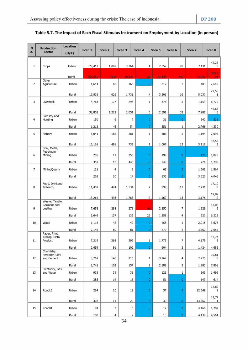
Assessing policy effectiveness during the crisis: The case of Indonesia DP 208
34
Table 5.7. The Impact of Each Fiscal Stimulus Instrument on Employment by Location (in person)
N
o.
Production
Sector
Location
Scen 1 Scen 2 Scen 3 Scen 4 Scen 5 Scen 6 Scen 7 Scen 8 (U/R)
1 Crops Urban
29,412
1,097
2,264
4
2,352
28
7,131
42,28
8
Rural
268,054
9,998
20,633
39
21,435
259
64,991
385,4
08
2
Other
Agriculture Urban
1,614
60
166
0
317
2
483
2,642
Rural
16,833
626
1,731
4
3,305
16
5,037
27,551
3 Livestock Urban
4,763
177
298
1
376
5
1,159
6,779
Rural
32,802
1,222
2,051
5
2,591
32
7,981
46,683
4 Forestry and Hunting Urban
150
6
7
0
31
0
342
536
Rural
1,212
46
54
0
251
1
2,766
4,330
5 Fishery Urban
5,041
188
281
1
386
5
1,194
7,095
Rural
13,161
491
733
2
1,007
13
3,119
18,525
6
Coal, Metal, Petroleum
Mining Urban
285
11
355
0
199
0
179
1,028
Rural
357
13
446
0
249
0
224
1,290
7 MiningQuarry Urban
121
4
8
0
62
0
1,668
1,864
Rural
263
10
17
0
135
0
3,620
4,045
8
Food, Drinkand
Tobacco Urban
11,407
424
1,534
2
999
11
2,731
17,10
8
Rural
13,264
493
1,783
2
1,162
13
3,176
19,89
2
9
Weave, Textile,
Garment and Leather Urban
7,658
288
278
46
2,850
7
1,929
13,056
Rural
3,649
137
132
22
1,358
4
920
6,222
10 Wood Urban
1,118
42
42
0
458
1
2,015
3,676
Rural
2,146
80
81
0
879
2
3,867
7,056
11
Paper, Print,
Transp, Metal Product Urban
7,219
268
299
1
1,773
7
4,179
13,746
Rural
2,459
91
102
0
604
2
1,424
4,683
12
Chemistry, Fertilizer, Clay and Cement Urban
3,767
140
216
1
3,962
4
2,725
10,81
5
Rural
2,741
102
157
1
2,882
3
1,983
7,868
13 Electricity, Gas and Water Urban
935
35
38
0
125
1
365
1,499
Rural
383
14
16
0
51
0
149
614
14 RoadLI Urban
284
10
19
0
37
0
12,549
12,89
9
Rural
302
11
20
0
39
0
13,367
13,74
1
15 RoadKI Urban
94
3
6
0
12
0
4,166
4,282
Rural
100
4
7
0
13
0
4,438
4,561
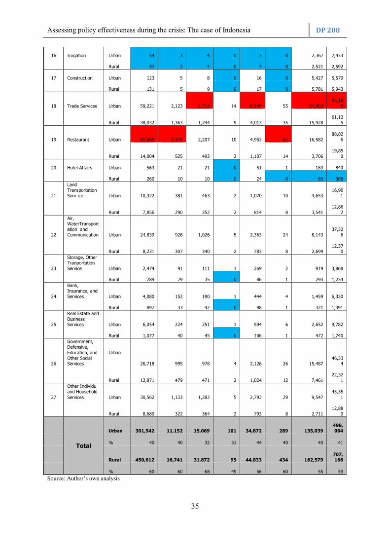
Assessing policy effectiveness during the crisis: The case of Indonesia DP 208
35
16 Irrigation Urban
54
2
4
0
7
0
2,367
2,433
Rural
57
2
4
0
7
0
2,521
2,592
17 Construction Urban
123
5
8
0
16
0
5,427
5,579
Rural
131
5
9
0
17
0
5,781
5,943
18 Trade Services Urban
59,221
2,123
2,716
14
6,249
55
24,803
95,180
Rural
38,032
1,363
1,744
9
4,013
35
15,928
61,125
19 Restaurant Urban
62,665
2,349
2,207
10
4,952
61
16,582
88,82
6
Rural
14,004
525
493
2
1,107
14
3,706
19,85
0
20 Hotel Affairs Urban
563
21
21
0
51
1
183
840
Rural
260
10
10
0
24
0
85
388
21
Land
Transportation Serv ice Urban
10,322
381
463
2
1,070
10
4,653
16,901
Rural
7,856
290
352
2
814
8
3,541
12,862
22
Air, WaterTransport
ation and Communication Urban
24,839
926
1,026
5
2,363
24
8,143
37,326
Rural
8,231
307
340
2
783
8
2,699
12,370
23
Storage, Other Tranportation
Service Urban
2,474
91
111
1
269
2
919
3,868
Rural
789
29
35
0
86
1
293
1,234
24
Bank, Insurance, and
Services Urban
4,080
152
190
1
444
4
1,459
6,330
Rural
897
33
42
0
98
1
321
1,391
25
Real Estate and
Business Services Urban
6,054
224
251
1
594
6
2,652
9,782
Rural
1,077
40
45
0
106
1
472
1,740
26
Government,
Defensive, Education, and
Other Social Services
Urban
26,718
995
978
4
2,126
26
15,487
46,334
Rural
12,871
479
471
2
1,024
12
7,461
22,32
1
27
Other Individu and Household
Services Urban
30,562
1,133
1,282
5
2,793
29
9,547
45,35
1
Rural
8,680
322
364
2
793
8
2,711
12,880
Total
Urban
301,542
11,152
15,069
101
34,872
289
135,039
498,
064
%
40
40
32
51
44
40
45
41
Rural
450,612
16,741
31,872
95
44,833
434
162,579
707,
166
%
60
60
68
49
56
60
55
59
Source: Author’s own analysis

Assessing policy effectiveness during the crisis: The case of Indonesia DP 208
36
Table 5.7 also suggest that sector that experiences relatively higher production activities does not always experience a higher employment impact and vice a versa, for instance electricity, gas and water sector, transportation sector, other agriculture sector and some services sectors. These are largely due to the characteristic of the sector. If a sector experiences higher production activities and the sector is capital intensive, the impact on the employment will be a relatively small since more capital is needed to increase the production. In Scenario 7 we can see that infrastructure stimulus will result more than 297,628 new jobs. The result is rational because infrastructure will employ a relatively large number of workers. However the impact is much smaller than the scenario 1 which can create approximately 0.75 million labour places. Important to note here that budget that are spent in this scenario is only less than half of personal tax cut policy. In scenario 8 we can see the total employment that can be created from the whole fiscal stimulus policy. It is estimated that at least 1.2 million new jobs could be created. However we should notice that the new jobs could be in formal or informal sector.

Assessing policy effectiveness during the crisis: The case of Indonesia DP 208
37
Table 5.8. The Impact of Each Fiscal Stimulus Instrument on Employment by Gender (in
persons)
No. Production Sector
Sex
Scen 1 Scen 2 Scen 3 Scen 4 Scen 5 Scen 6 Scen 7 Scen 8 (M/W)
1 Crops Men
176,262
6,574
13,567
26
14,095
170
42,735
253,430
Women
121,203
4,521
9,329
18
9,692
117
29,386
174,267
2 Other Agriculture Men
11,956
445
1,229
3
2,347
12
3,577
19,569
Women
6,491
242
667
2
1,274
6
1,942
10,624
3 Livestock Men
21,935
817
1,372
3
1,732
21
5,337
31,217
Women
15,631
582
977
2
1,234
15
3,803
22,245
4 Forestry and Hunting Men
1,077
40
48
0
223
1
2,458
3,848
Women
285
11
13
0
59
0
651
1,018
5 Fishery Men
16,572
618
923
2
1,268
16
3,927
23,326
Women
1,630
61
91
0
125
2
386
2,294
6
Coal, Metal,
Petroleum Mining Men
602
22
751
0
420
1
378
2,174
Women
40
1
50
0
28
0
25
144
7 MiningQuarry Men
281
10
18
0
145
0
3,867
4,321
Women
103
4
6
0
53
0
1,421
1,587
8 Food, Drinkand Tobacco Men
11,525
428
1,549
2
1,009
11
2,760
17,284
Women
13,146
489
1,767
2
1,151
13
3,148
19,716
9
Weave, Textile, Garment and
Leather Men
4,489
169
163
27
1,670
4
1,131
7,653
Women
6,818
256
247
41
2,537
7
1,718
11,625
10 Wood Men
1,953
73
74
0
800
2
3,519
6,420
Women
1,311
49
50
0
537
1
2,363
4,312
11 Paper, Print, Transp, Metal Product Men
7,264
270
301
1
1,784
7
4,205
13,832
Women
2,414
90
100
0
593
2
1,398
4,597
12 Chemistry, Fertilizer, Clay and Cement Men
4,539
168
260
2
4,773
4
3,284
13,030
Women
1,969
73
113
1
2,071
2
1,425
5,654
13
Electricity, Gas and
Water Men
1,205
45
49
1
161
1
470
1,932
Women
113
4
5
0
15
0
44
181
14 RoadLI Men
572
21
38
0
75
1
25,308
26,015
Women
14
1
1
0
2
0
608
625
15 RoadKI Men
190
7
13
0
25
0
8,401
8,636
Women
5
0
0
0
1
0
202
208
16 Irrigation Men
108
4
7
0
14
0
4,773
4,907
Women
3
0
0
0
0
0
115
118
17 Construction Men
248
9
16
0
32
0
10,946
11,251
Women
6
0
0
0
1
0
263
270
18 Trade Services Men
49,343
1,769
2,263
12
5,206
46
20,666
79,304
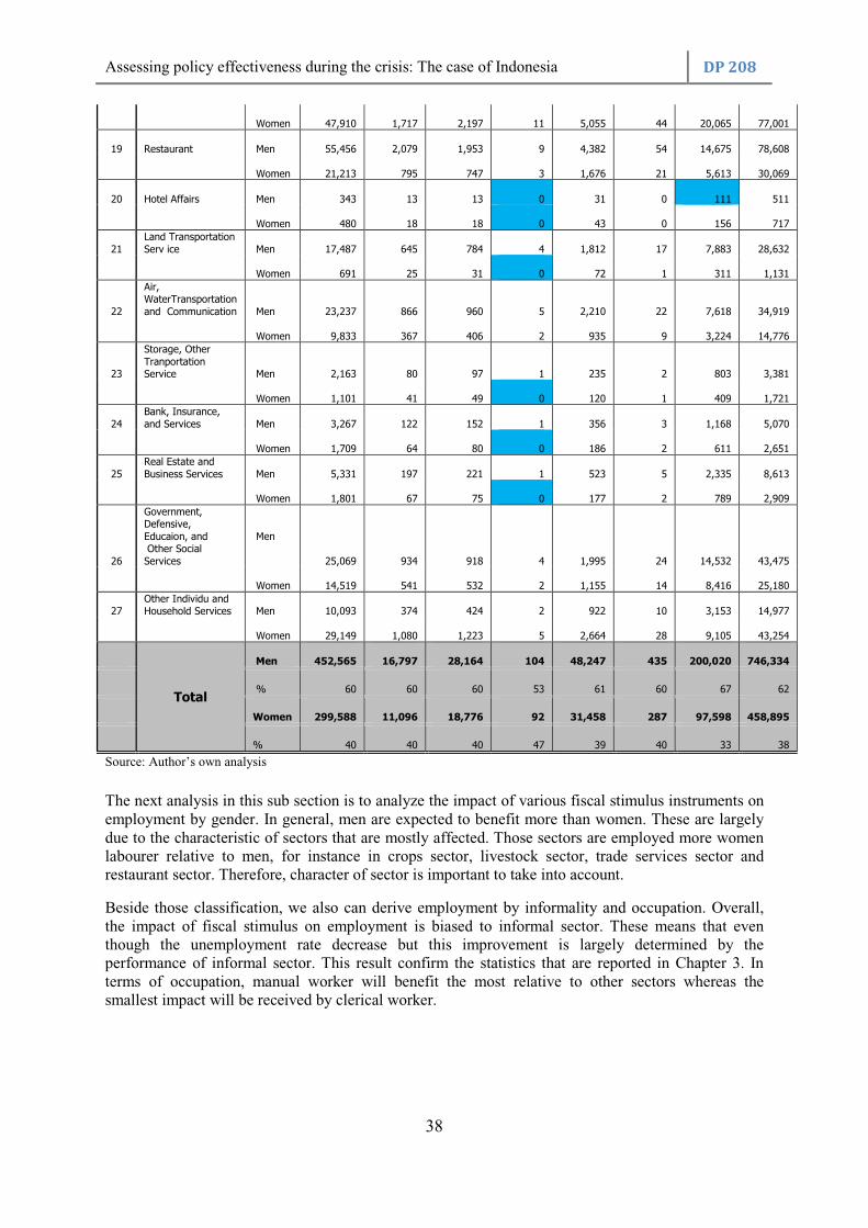
Assessing policy effectiveness during the crisis: The case of Indonesia DP 208
38
Women
47,910
1,717
2,197
11
5,055
44
20,065
77,001
19 Restaurant Men
55,456
2,079
1,953
9
4,382
54
14,675
78,608
Women
21,213
795
747
3
1,676
21
5,613
30,069
20 Hotel Affairs Men
343
13
13
0
31
0
111
511
Women
480
18
18
0
43
0
156
717
21
Land Transportation
Serv ice Men
17,487
645
784
4
1,812
17
7,883
28,632
Women
691
25
31
0
72
1
311
1,131
22
Air, WaterTransportation
and Communication Men
23,237
866
960
5
2,210
22
7,618
34,919
Women
9,833
367
406
2
935
9
3,224
14,776
23
Storage, Other
Tranportation Service Men
2,163
80
97
1
235
2
803
3,381
Women
1,101
41
49
0
120
1
409
1,721
24
Bank, Insurance,
and Services Men
3,267
122
152
1
356
3
1,168
5,070
Women
1,709
64
80
0
186
2
611
2,651
25
Real Estate and
Business Services Men
5,331
197
221
1
523
5
2,335
8,613
Women
1,801
67
75
0
177
2
789
2,909
26
Government, Defensive,
Educaion, and Other Social
Services
Men
25,069
934
918
4
1,995
24
14,532
43,475
Women
14,519
541
532
2
1,155
14
8,416
25,180
27 Other Individu and Household Services Men
10,093
374
424
2
922
10
3,153
14,977
Women
29,149
1,080
1,223
5
2,664
28
9,105
43,254
Total
Men
452,565
16,797
28,164
104
48,247
435
200,020
746,334
%
60
60
60
53
61
60
67
62
Women
299,588
11,096
18,776
92
31,458
287
97,598
458,895
%
40
40
40
47
39
40
33
38
Source: Author’s own analysis
The next analysis in this sub section is to analyze the impact of various fiscal stimulus instruments on employment by gender. In general, men are expected to benefit more than women. These are largely due to the characteristic of sectors that are mostly affected. Those sectors are employed more women labourer relative to men, for instance in crops sector, livestock sector, trade services sector and restaurant sector. Therefore, character of sector is important to take into account.
Beside those classification, we also can derive employment by informality and occupation. Overall, the impact of fiscal stimulus on employment is biased to informal sector. These means that even though the unemployment rate decrease but this improvement is largely determined by the performance of informal sector. This result confirm the statistics that are reported in Chapter 3. In terms of occupation, manual worker will benefit the most relative to other sectors whereas the smallest impact will be received by clerical worker.

Assessing policy effectiveness during the crisis: The case of Indonesia DP 208
39
Table 5.9. The Impact of Each Fiscal Stimulus Instrument on Employment by Informality and
Occupation (in persons)
Source: Author’s own analysis
Based on the result above, we can take some important findings. First, the impact of fiscal stimulus policy on employment will be biased to worker in rural area, men and informal sector. Second, crops sector seem to received highest impact for any scenario in terms of number of jobs that are created. This is rational since crops sector is a labor intensive sector and the impact of all scenario are relatively larger on crops activities that will derive higher demand on labour. Third, the impact of extra government budget on infrastructure will not only increase number of worker in construction related sector but also other sectors and even larger on crops sector, restaurant sector and trade services sector.
5. 5. The Net Cost of the Fiscal Stimulus
As previously mentioned, the Government used several types of fiscal stimulus instruments that were grouped into seven scenarios. In the first scenario, the Government decreased the personal income tax rate, which equaled to 24.7 trillion IDR decrease in government tax revenue. Based on SAM approach, the policy is expected to improve Indonesian economic performance including production activity, factor’s income and household income. Consequently, government income from taxes and tariff will increase. This is also the case for the rest of scenarios. This implies that even though in the fiscal stimulus policies increased government spending and reduced their revenue, the improvement on economic activity or household will result more government income than the baseline condition. Based on those argument, the net cost of each fiscal stimulus instrument should be considered. However, the injections that are used in the eight scenarios are differ one to another. Thus, we cannot compare the output of net cost directly.
Table 5.10. The Net Cost of the Fiscal Stimulus
Source: Author’s own analysis
Labour by Occupation and Informality Scen 1 Scen 2 Scen 3 Scen 4 Scen 5 Scen 6 Scen 7 Scen 8
Formal Agricultural Worker 9,032.06 336.79 683.49 1.36 779.55 8.73 2,268.90 13,110.87
Informal Agricultural Worker 309,983.87 11,558.63 23,457.70 46.78 26,754.32 299.45 77,869.46 449,970.21
Formal Manual Worker 139,641.82 5,158.61 7,409.45 47.24 16,722.32 133.64 69,463.92 238,577.00
Informal Manual Worker 228,495.42 8,441.02 12,124.06 77.29 27,362.67 218.68 113,663.56 390,382.70
Formal Clerical Worker 7,740.15 285.62 389.30 2.79 962.96 7.40 4,094.17 13,482.39
Informal Clerical Worker 19,109.38 705.15 961.13 6.89 2,377.42 18.27 10,107.95 33,286.19
Formal Professional Worker 32,497.13 1,199.06 1,631.23 11.77 4,042.66 31.06 17,164.07 56,576.99
Informal Professional Worker 5,653.80 208.61 283.80 2.05 703.34 5.40 2,986.18 9,843.18
Total 752,153.62 27,893.49 46,940.17 196.18 79,705.23 722.63 297,618.21 1,205,229.53
Labour by Occupation
Agricultural Worker 319,015.93 11,895.42 24,141.19 48.15 27,533.87 308.17 80,138.36 463,081.08
Manual Worker 368,137.24 13,599.64 19,533.52 124.53 44,084.98 352.32 183,127.48 628,959.71
Clerical Worker 26,849.52 990.76 1,350.43 9.69 3,340.38 25.67 14,202.13 46,768.57
Professional Worker 38,150.93 1,407.67 1,915.03 13.82 4,746.00 36.47 20,150.25 66,420.17
Total 752,153.62 27,893.49 46,940.17 196.18 79,705.23 722.63 297,618.21 1,205,229.53
Labour by Informality
Formal 188,911.16 6,980.08 10,113.48 63.16 22,507.48 180.83 92,991.06 321,747.25
Informal 563,242.46 20,913.41 36,826.69 133.02 57,197.75 541.80 204,627.16 883,482.28
Total 752,153.62 27,893.49 46,940.17 196.18 79,705.23 722.63 297,618.21 1,205,229.53
scen 1 scen 2 scen 3 scen 4 scen 5 scen 6 scen 7 scen 8
Gov Income 5,749.03 2,659.38 556.61 1.43 684.11 68.90 2,320.66 12,034.74
Govt Injection 24,707.27 19,300.00 1,834.93 7.19 4,157.80 500.00 10,913.23 61,420.43
Net Cost 18,958.24 16,640.62 1,278.32 5.76 3,473.69 431.10 8,592.57 49,385.69
B/C Ratio 23% 14% 30% 20% 16% 14% 21% 20%
Assessing policy effectiveness during the crisis: The case of Indonesia DP 208
40
An alternative solution that can be used is Benefit Cost Ratio (B/C Ratio) concept. B/C Ratio can give us an information regarding how much benefit that can be earned by government relative to the cost or budget that are spent. Among 8 scenario, indirect tax scenario will give the largest B/C ratio. If government decrease the indirect tax, sectors will develop and have more incentive to produce more. As a result, output will increase and then raise the government income from the indirect tax. Moreover, more labor and capital will be employed and result higher factor income. Consequently, household income will increase as well as the government income from income tax. Both the raise of indirect tax and income tax will increase government income.
Chapter 6: Conclusion
Employment satellite account is a very useful feature in DySAM, particularly to estimate the impact of policy scenarios on the employment. However, the accuracy of the employment data is strongly important in determining the impact, as is a good methodology for calculating the satellite account. In Indonesia, there are two sources of employment data, namely LFS and Labour Statistic of SAM. Each source uses different definition of labour. In LFS, labour is defined as the economically active population aged 15 and over, whereas in SAM, labour is defined as economically active population aged 10 and over. In terms of number of sectors, LFS classified labour by 9 sectors whereas SAM disaggregate labour by 24 sectors. Another difference is the time period. Number of labours in SAM is calculated at the end of the year of SAM publication (December) whereas the one that published in LFS is calculated at February or August. Time is matters in employment data since employment in particular sector has specific trend, for instance agriculture. If we conduct labour survey in the harvesting time, number of labour will substantially large in agriculture and vice a versa. Thus, if we want to conduct SAM analysis by using employment satellite, we must be convinced that the structure of employment data is perfectly matched with the SAM structure. There are two important points that should be considered if we want to use Indonesian employment data in SAM analysis. First, if the analysis is conducted at the same period with year of SAM publication, SAM-based employment data is more appropriate than LFS-based employment data. Second, if the analysis is conducted at the period that is not the same with year of SAM publication, we should do some adjustment on the employment data. In this study we propose alternative approach to adjust employment data that is presented in this study.
One of the benefits of DySAM with employment satellite is to analyze the impact of fiscal stimulus policy (FSP) on Indonesian macroeconomic indicators, namely sectoral output, labour income, household income and employment by location and gender. Overall, the realization rates of FSP in Indonesia achieved 83.84 per cent from its total budget. There are number of factors that cause this low realization rates, namely decision lag, implementation lag, regulation problem, administration problem and timely tender process. Based on result of policy scenario in DySAM analysis, we can conclude that the impact of each fiscal stimulus is differs from one to another. These are largely determined by type of FSP tools that are used and the characteristic of sector in which FSP is implemented. Therefore, in formulating fiscal stimulus programs, government should consider the tools and transmission mechanism of each tool to estimate the impact of each FSP instrument and then match the predicted output with the government objective.
In order to get an accurate estimation, we must ensure that a shock or injection procedure in the model is appropriate. There are three important points that should be considered in the management of shocks. First, we should be convinced that the data or magnitudes that are used for injection is correct. Second, we should ensure that mapping procedure between real data and SAM structure is appropriate and has good precision. Third, after mapping procedure, we should allocate the magnitude or size of injection (shock) on more detail account in SAM. In this step, we should convince that approach we have used is appropriate and in line with the description of scenario. For instance if we want to simulate the personal tax cut, we will face two options, whether to allocate the tax cut evenly or proportionally on ten types of households in SAM structure.
Assessing policy effectiveness during the crisis: The case of Indonesia DP 208
41
Chapter 7: Policy implication
Seven scenarios that have been presented previously could provide Government of Indonesia a very useful information regarding the impact of each and all fiscal stimulus instrument on Indonesian economic performance. All scenarios are designed based on the document of Ministry of Finance and used the realization value as the shocks. There are some lessons that can be drawn from the results. First, since the fiscal stimulus policy use either tax reduction or expansive government spending, the impact on Indonesian economic performance will be positive. However the magnitude and the most affected “stakeholders” will be differ across fiscal stimulus instrument. Second, any scenario will result a moderate and even a relatively higher impact on agricultural sector if the stimulus is conducted through personal tax cut or corporate income tax cut. Even though the main objective of some fiscal stimulus instrument are to improve the competitiveness of manufacturing sector but agricultural sector -as the primary sector- will benefit from the second round effect of the stimulus. Third, fiscal stimulus policy through subsidy and value added tax reduction seems to be the most appropriate instrument to increase the competitiveness of manufacturing industry. However, the size of fiscal stimulus budget is matters which can be seen from a relatively low impact of value added tax cut policy. If government focus to improve the performance of manufacturing industry, Government of Indonesia should allocate more budget on these two instruments, namely subsidy and value added tax reduction. Fourth, construction sector, road sector and irrigation sector is expected to benefit the most if the fiscal stimulus policy is conducted through an expansion of government budget on infrastructure. These four important findings imply that the best fiscal stimulus policy to respond the Global Financial Crisis 2008 is conducted through mix policy since the impact of the crisis is existed in almost all sectors.
Another important lesson can also be drawn in terms of the impact of fiscal stimulus on factor’s income. Type of production factor that will received the largest impact will significantly depend on the characteristic of sector that benefit from the stimulus. For instance, if the construction sector is one of sectors that received the highest benefit due to the fiscal stimulus, type of worker that is expected to benefit the most will be manual worker. This is largely due to the characteristic of construction sector that employ more manual worker relative to others.
One of the most interesting findings is on the impact of fiscal stimulus on household income. It is expected that the benefit of fiscal stimulus policy will be bias to medium-high income household. The argument is due to type of sector that received the fiscal stimulus. If government want to support the low income household (agriculture employee, rural low income and urban low income), government should impose the fiscal stimulus policy on the sector that employ worker from a low income household groups, for instance agricultural sector, and trade sector.
Gender, location, occupation and informality are another focus in this study. In line with the impact on the activities, labour in the crops sector seems to benefit the most in any scenario. In terms of occupation, we can simply conclude that the impact will be a relatively larger on agricultural worker and manual worker and it has been justified by the result in this study. Crops sector is mostly located in rural area, thus the impact of fiscal stimulus is significantly higher for employment in rural area. Since the structure of employment in Indonesia is majorly dominated by informal worker and mostly are men, the impact of fiscal stimulus is expected to biased to informal worker particularly on men worker.

Assessing policy effectiveness during the crisis: The case of Indonesia DP 208
42
ANNEX
Annex 1. Indonesian Economic Performance before and during the Crisis
Indicators 1996 1997 1998 2007 2008 2009 GDP growth: 1st Quartile 2nd Quartile 3rd Quartile 4th Quartile
5.97 % 6.81 % 7.62 % 9.64 %
7.44 % 6.11 % 4.46 % -0.92 %
-7.14 % -15.94 % -17.45 % -19.39 %
6.06 % 6.73 % 6.74 % 5.84 %
6.21% 6.30% 6.25% 5.27%
4.53% 4.08% 4.16% 5.43%
GDP by Sector Agriculture Mining Manufacturing Electricity, Gas & Water Construction Trade, Hotel & Restaurant Transport & Communication Finance Other Services
3.05% 4.73% 8.77% 14.27% 12.75% 11.26% 13.02% 5.95% 3.44%
0.81% 1.14% 2.41% 13.81% 7.36% 8.28% 10.76% 6.07% 3.97%
-2.96% -1.68% -20.53% 1.75% -36.44% -17.71% -9.91% -24.03% -3.23%
3.47% 1.93% 4.67% 10.33% 8.53% 8.93% 14.04% 7.99% 6.44%
4.83% 0.68% 3.66% 10.92% 7.51% 6.87% 16.57% 8.24% 6.23%
4.13% 4.37% 2.11% 13.78% 7.05% 1.14% 15.53% 5.05% 6.40%
Inflation rate 6.6 % 11.6 % 77.6 % 11.6 % 11.06% 2.78% Unemployment rate 4.89 % 4.68% 5.46% 9.1 % 8.39 % 7.9%
Employment Total 85,701,813 87,049,756 87,672,449
(Feb) 97,583,141 (Aug) 99,930,217
(Feb) 102,049,857 (Aug) 102,552,750
(Feb) 104,485,444 (Aug) 104,870,663
Share of Formal Employment n.a. n.a. n.a. (Feb) 27.5% (Aug) 28.1%
(Feb) 27.9% (Aug) 27.5%
(Feb) 27.7% (Aug) 27.8%
Share of Informal Employment
n.a. n.a. n.a. (Feb) 72.5% (Aug) 71.9%
(Feb) 72.1% (Aug) 72.5%
(Feb) 72.3% (Aug) 72.2%
Underemployment (million people)
n.a. n.a. n.a. (Feb) 30.2 (Aug) 30.4
(Feb) 30.6 (Aug) 31.1
(Feb) 31.4 (Aug) 31.6
Sector that suffer the most in terms of impact on labour
Industry Industry Industry Industry
Private Consumption per capita
n.a. n.a. n.a. 353,421 386,370 430,065
Growth of Household Consumption
5.9% -4.1% 5.01% 5.34% 4.85%
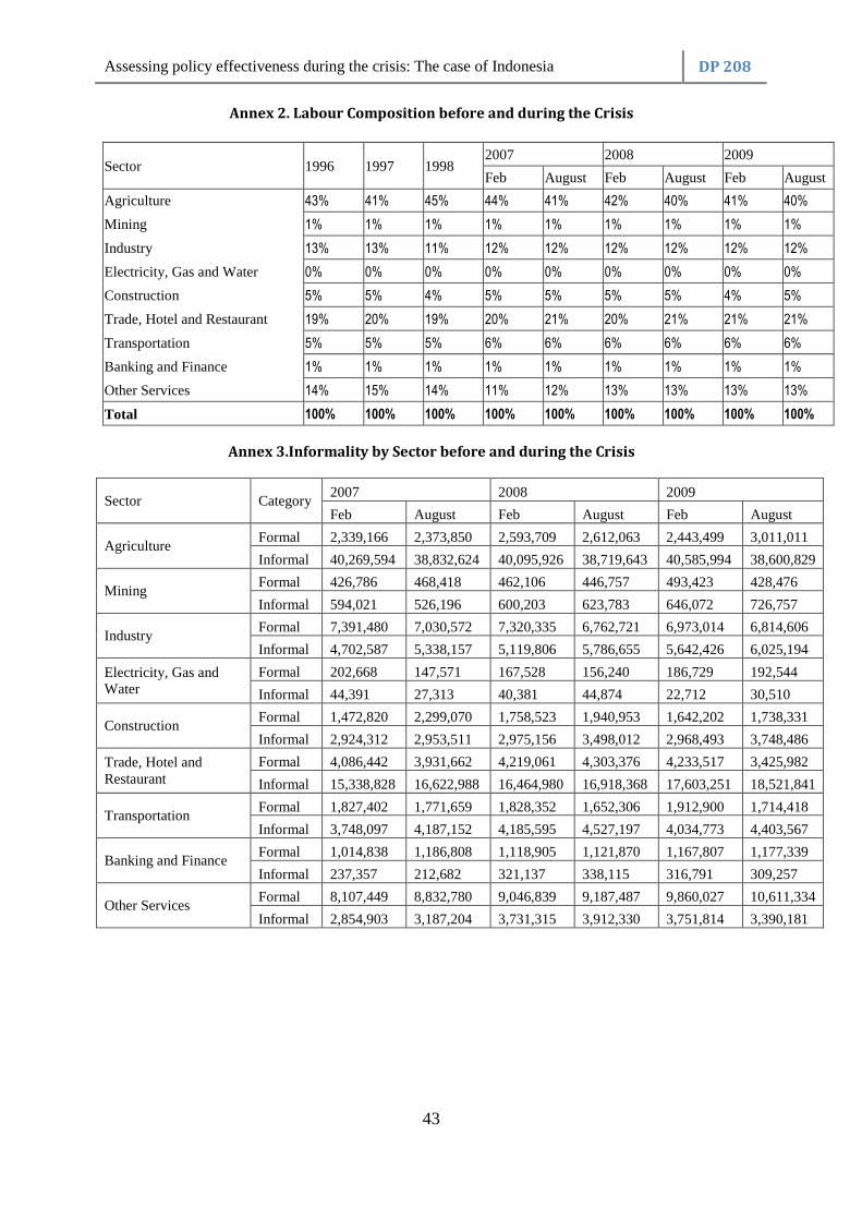
Assessing policy effectiveness during the crisis: The case of Indonesia DP 208
43
Annex 2. Labour Composition before and during the Crisis
Sector 1996 1997 1998 2007 2008 2009
Feb August Feb August Feb August
Agriculture 43% 41% 45% 44% 41% 42% 40% 41% 40%
Mining 1% 1% 1% 1% 1% 1% 1% 1% 1%
Industry 13% 13% 11% 12% 12% 12% 12% 12% 12%
Electricity, Gas and Water 0% 0% 0% 0% 0% 0% 0% 0% 0%
Construction 5% 5% 4% 5% 5% 5% 5% 4% 5%
Trade, Hotel and Restaurant 19% 20% 19% 20% 21% 20% 21% 21% 21%
Transportation 5% 5% 5% 6% 6% 6% 6% 6% 6%
Banking and Finance 1% 1% 1% 1% 1% 1% 1% 1% 1%
Other Services 14% 15% 14% 11% 12% 13% 13% 13% 13%
Total 100% 100% 100% 100% 100% 100% 100% 100% 100%
Annex 3.Informality by Sector before and during the Crisis
Sector Category 2007 2008 2009
Feb August Feb August Feb August
Agriculture Formal 2,339,166 2,373,850 2,593,709 2,612,063 2,443,499 3,011,011
Informal 40,269,594 38,832,624 40,095,926 38,719,643 40,585,994 38,600,829
Mining Formal 426,786 468,418 462,106 446,757 493,423 428,476
Informal 594,021 526,196 600,203 623,783 646,072 726,757
Industry Formal 7,391,480 7,030,572 7,320,335 6,762,721 6,973,014 6,814,606
Informal 4,702,587 5,338,157 5,119,806 5,786,655 5,642,426 6,025,194
Electricity, Gas and Water
Formal 202,668 147,571 167,528 156,240 186,729 192,544
Informal 44,391 27,313 40,381 44,874 22,712 30,510
Construction Formal 1,472,820 2,299,070 1,758,523 1,940,953 1,642,202 1,738,331
Informal 2,924,312 2,953,511 2,975,156 3,498,012 2,968,493 3,748,486
Trade, Hotel and Restaurant
Formal 4,086,442 3,931,662 4,219,061 4,303,376 4,233,517 3,425,982
Informal 15,338,828 16,622,988 16,464,980 16,918,368 17,603,251 18,521,841
Transportation Formal 1,827,402 1,771,659 1,828,352 1,652,306 1,912,900 1,714,418
Informal 3,748,097 4,187,152 4,185,595 4,527,197 4,034,773 4,403,567
Banking and Finance Formal 1,014,838 1,186,808 1,118,905 1,121,870 1,167,807 1,177,339
Informal 237,357 212,682 321,137 338,115 316,791 309,257
Other Services Formal 8,107,449 8,832,780 9,046,839 9,187,487 9,860,027 10,611,334
Informal 2,854,903 3,187,204 3,731,315 3,912,330 3,751,814 3,390,181

Assessing policy effectiveness during the crisis: The case of Indonesia DP 208
44
Annex 4. Government Fiscal Stimulus 2009 (billion IDR)
Policy Instruments Budget
I. Tax Cut 56,300.0 a. Personal Income 31,000.0 b. Corporate Income 19,300.0 c. Value Added Tax 3,500.0 - Cooking Oil 800.0 - Biofuels 200.0 - Oil and Gas Exploration 2,500.0 d. Tariff Import 2,500.0 - Airplane 416.0
- Vehicle 795.2 - Electronic 215.4 - Shipping 151.0 - Heavy equipment 106.0 - Infusion 11.4 - Water generated power plant 14.0 - Sorbitol 0.7 - Telematics 50.0 - Methyl 0.9 - Pen 3.2 - Others 736.2 II. Government Spending 16,958.5 a. Subsidies 4,522.8 - Clean Water 15.0 - Medicines 350.0 - Diesel fuel 2,779.9 - Electricity for food industry 82.7 - Electricity for textile industry 344.5 - Electricity for wood industry 68.9
- Electricity for paper industry 578.7
- Electricity for chemical industry 303.1
b. Government Transfer to Corporate 500.0
- Jamkrindo and Askrindo 500.0
c. Infrastructure Expenditure 11,935.7 - Infrastructure for flood control in Bengawan Solo 700.0 - Rehabilitation food security network 461.0 - Distribution network and installation of drinking water 450.0 - Acceleration of multi years project 900.0 - Road, bridge and irrigation 3,423.2 - Housing 243.0
- Inspection road and irrigation 424.0 - Railway 300.0 - Airport 714.0 - Extension of airport runway 145.2 - Revitalization of railroad system 100.0
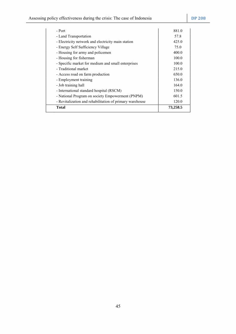
Assessing policy effectiveness during the crisis: The case of Indonesia DP 208
45
- Port 881.0 - Land Transportation 57.8 - Electricity network and electricity main station 425.0 - Energy Self Sufficiency Village 75.0 - Housing for army and policemen 400.0 - Housing for fisherman 100.0 - Specific market for medium and small enterprises 100.0 - Traditional market 215.0 - Access road on farm production 650.0 - Employment training 136.0 - Job training hall 164.0 - International standard hospital (RSCM) 150.0 - National Program on society Empowerment (PNPM) 601.5 - Revitalization and rehabilitation of primary warehouse 120.0
Total 73,258.5

Assessing policy effectiveness during the crisis: The case of Indonesia DP 208
46
Annex 5. New Estimates of Employment
Sectors 2005 2006 2007 2008
Crops 31,814,800 30,676,471 30,638,909 30,527,137
Other Agriculture 5,615,930 4,510,376 3,536,325 3,452,175
Livestock 2,447,670 2,532,195 3,303,705 3,407,475
Forestry 504,050 608,293 585,130 635,565
Fishery 1,625,280 1,577,043 1,835,992 1,775,711
Coal, Metal, Petroleum Mining 314,940 347,491 359,276 394,512
Mining and Quarry 550,730 517,510 607,137 611,464
Food, Beverages and Tobacco 2,433,250 2,665,828 2,651,551 2,673,431
Textile, Wearing apparel, Garment and Leather
2,806,210 2,713,336 2,591,724 2,636,927
Wood 2,388,440 2,140,502 2,117,101 1,987,930
Paper, Print, Transp, Metal Product, other industry
2,511,380 2,314,682 2,668,504 2,687,494
Chemical, Fertilizer, Clay and Cement 1,732,490 1,769,089 1,857,509 1,986,709
Electricity, Gas and Water 191,190 219,507 163,706 187,709
RoadLI 2,246,912 2,331,372 2,517,961 2,657,921
RoadKI 800,673 751,850 866,400 837,883
Irrigation 449,971 445,913 495,491 485,982
Construction 1,000,004 1,000,518 1,047,743 1,105,860
Trade Services 16,226,480 16,528,646 15,323,415 15,869,948
Restaurant 2,076,660 3,482,202 8,127,491 8,159,323
Hotel Affairs 190,510 211,818 222,450 237,433
Land Transportation Services 3,365,410 3,189,497 3,011,323 3,046,302
Air, Water Transportation and Communication
1,705,540 1,816,219 2,140,932 2,672,169
Storage, Other Transportation Service 540,110 664,352 971,010 978,121
Bank, Insurance, and Services 541,460 647,236 686,320 639,501
Real Estate and Business Services 904,060 1,010,097 972,040 1,128,659
Government, Defensive, Education, and 6,502,620 7,043,591 7,090,888 6,866,101
Other Individual and Household Services 3,977,090 4,258,318 4,552,102 5,801,244
Source: Author’s own analysis

Assessing policy effectiveness during the crisis: The case of Indonesia DP 208
47
Annex 6. New Estimates of Productivity
Sector 2005 2006 2007 2008
Crops 7046 7531 9010 11704
Other Agriculture 16942 21738 33139 43928
Livestock 27579 27471 25167 31575
Forestry 51881 44301 55046 65578
Fishery 44325 47073 48328 64661
Coal, Metal, Petroleum Mining 1076518 1005413 1162300 1369698
Mining and Quarry 63709 69865 71179 91454
Food, Beverages and Tobacco 211436 198871 238981 306713
Textile, Wearing apparel, Garment and Leather 80346 85629 107150 136277
Wood 34888 40116 48478 66808
Paper, Print, Transp, Metal Product, other industry 274872 307320 318620 409385
Chemical, Fertilizer, Clay and Cement 355530 361635 398471 488813
Electricity, Gas and Water 503378 455437 706219 808248
RoadLI 34467 34230 37882 46439
RoadKI 221702 243295 252351 337659
Irrigation 495210 514948 553907 730786
Construction 93172 95962 109529 134284
Trade Services 30542 30897 39834 49771
Restaurant 91606 56296 28829 37160
Hotel Affairs 148558 137685 156703 189980
Land Transportation Services 47027 51143 64698 82784
Air, Water Transportation and Communication 117071 113313 114789 119055
Storage, Other Transportation Service 70229 58835 48114 61807
Bank, Insurance, and Services 320313 276133 311252 432252
Real Estate and Business Services 192184 177252 220155 245351 Government, Defensive, Education, and Social Services 46592 44327 52619 70324
Other Individual and Household Services 42027 40448 45225 45921 Source: Author’s own analysis
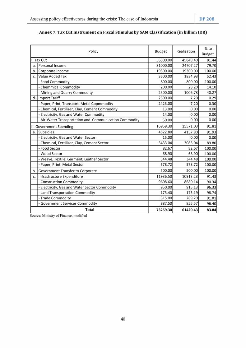
Assessing policy effectiveness during the crisis: The case of Indonesia DP 208
48
Annex 7. Tax Cut Instrument on Fiscal Stimulus by SAM Classification (in billion IDR)
Source: Ministry of Finance, modified
Policy Budget Realization % to
Budget
I. Tax Cut 56300.00 45849.40 81.44
a. Personal Income 31000.00 24707.27 79.70
b. Corporate Income 19300.00 19300.00 100.00
c. Value Added Tax 3500.00 1834.93 52.43
- Food Commodity 800.00 800.00 100.00
- Chemmical Commodity 200.00 28.20 14.10
- Mining and Quarry Commodity 2500.00 1006.73 40.27
d. Import Tariff 2500.00 7.20 0.29
- Paper, Print, Transport, Metal Copmmodity 2423.00 7.20 0.30
- Chemical, Fertilizer, Clay, Cement Commodity 13.00 0.00 0.00
- Electricity, Gas and Water Commodity 14.00 0.00 0.00
- Air-Water Transportation and Communication Commodity 50.00 0.00 0.00
II. Government Spending 16959.30 15571.03 91.81
a. Subsidies 4522.80 4157.80 91.93
- Electricity, Gas and Water Sector 15.00 0.00 0.00
- Chemical, Fertilizer, Clay, Cement Sector 3433.04 3083.04 89.80
- Food Sector 82.67 82.67 100.00
- Wood Sector 68.90 68.90 100.00
- Weave, Textile, Garment, Leather Sector 344.48 344.48 100.00
- Paper, Print, Metal Sector 578.72 578.72 100.00
b. Government Transfer to Corporate 500.00 500.00 100.00
c. Infrastructure Expenditure 11936.50 10913.23 91.43
- Construction Commodity 9608.60 8680.14 90.34
- Electricity, Gas and Water Sector Commodity 950.00 915.13 96.33
- Land Transportation Commodity 175.40 173.19 98.74
- Trade Commodity 315.00 289.20 91.81
- Government Services Commodity 887.50 855.57 96.40
73259.30 61420.43 83.84Total
Assessing policy effectiveness during the crisis: The case of Indonesia DP 208
49
References
Central Agency of Statistics (Badan Pusat Statistik or BPS), 2008. Social Accounting Matrix
2005. BPS Statistics Indonesia, Jakarta.
____________, 1997. Statistical Year Book of Indonesia 1997. Jakarta: BPS.
____________, 1998. Statistical Year Book of Indonesia 1998. Jakarta: BPS.
____________, 1999. Statistical Year Book of Indonesia 1999. Jakarta: BPS.
____________, 2007. Statistical Year Book of Indonesia 2007. Jakarta: BPS.
____________, 2008. Statistical Year Book of Indonesia 2008. Jakarta: BPS.
____________, 2009. Statistical Year Book of Indonesia 2009. Jakarta: BPS.
____________, 2010. Official Statistical Report No. 52/08/Th. XIII. 5 Agustus 2010
Central Bank of Indonesia (Bank Sentral Indonesia or BI). 1998. Indonesian Yearly
Economic Report 1997. Jakarta: BI
____________, 1999. Indonesian Yearly Economic Report 1998. Jakarta: BI
____________, 2008. Indonesian Yearly Economic Report 2007. Jakarta: BI
____________, 2009. Indonesian Yearly Economic Report 2008. Jakarta: BI
____________, 2010. Indonesian Yearly Economic Report 2009. Jakarta: BI
Defourny, J. and Thorbecke, E., 1984. Structural path analysis and multiplier decomposition
within a social accounting matrix framework. Economic Journal 94, 111-136.
Hartono, D. and Resosudarmo, B.P., 1998. Eksistensi matriks pengganda dan dekomposisi
matriks pengganda Pyatt dan Round dari sistem neraca sosial ekonomi. Ekonomi dan
Keuangan Indonesia 46 (4), 473-496.
ILO and CMEA., 2010. Indonesia Dynamic SAM Report: Concept, Methodology, Analysis
and Policy Design. Jakarta: ILO (unpublished).

Assessing policy effectiveness during the crisis: The case of Indonesia DP 208
50
Recent Discussion Paper Series Titres récents dans la série Documents de travail Títulos recientes en la serie Documentos de trabajo
Using the social capital of nationals abroad as a strategy for development in the IT sector, by Eric A. Charest. No. 172. 2007. ISBN 978-92-9014-820-3.
Los derechos sociales en el marco de las reformas laborales en América Latina, by Adrián
Goldin. No. 173. 2007. ISBN 978-92-9014-822-7. The Southern European social model: Changes and continuities in recent decades, by
Maria Karamessini. No. 174. 2007. ISBN 978-92-9014-832-6. The quest for a fair globalization three years on: Assessing the impact of the World
Commission on the Social Dimension of Globalization, by Hamish Jenkins, Eddy Lee, and Gerry Rodgers. No. 175. 2007. ISBN 978-92-9014-828-9.
Labour laws in South Asia: The need for an inclusive approach, by Kamala Sankaran. No.
176. 2007. ISBN 978-92-9014-830-2. L’effectivité du droit du travail et l’aspiration au travail décent dans les pays en dévelop- pement: une grille d’analyse, by Rachid Filali Meknassi. No. 177. 2007. ISBN 978-92-
9014-838-8. Globalization, the impact of trade liberalization, and labour law: The case of South Africa,
by Jan Theron, Shane Godfrey and Margareet Visser. No. 178. 2007. ISBN 978-92-9014-834-0.
Trade liberalization, labour law, and development: A contextualization, by Adelle Blackett.
No. 179. 2007. ISBN 978-92-9014-846-3. Labour law:A Southern African perspective, by Colin Fenwick, Evance Kalula and Ingrid
Landau. No. 180. 2007. ISBN 978-92-9014-842-5. La efectividad de la legislación laboral en América Latina, by Graciela Bensusán. No. 181.
2007. ISBN 978-92-9014-840-1. Gouvernance, droit international et responsabilité sociétale des entreprises Governance,
International Law and Corporate Societal Responsibility, edited by Jean-Claude Javillier. No. 182. 2007. ISBN 978-92-9014-836-4.
Issues in the analysis of global value chains and their impact on employment and incomes
in India, by Dev Nathan and V. Kalpana. No. 183. 2007. ISBN 978-92-9014-844-9. Explaining non-compliance with labour legislation in Latin America: A cross-country
analysis, by Adriana Marshall. No. 184. 2007. ISBN 978-92-9014-848-7.

Assessing policy effectiveness during the crisis: The case of Indonesia DP 208
51
Corporate social responsibility in multinational companies: Management initiatives or negotiated agreements? by Tony Edwards, Paul Marginson, Paul Edwards, Anthony Ferner, and Olga Tregaskis. No. 185. 2007. ISBN 978-92-9014-856-2.
The influence of the EU on the evolution of national employment models, by Jill Rubery,
Gerhard Bosch, and Steffen Lehndorff. No. 186. 2008. ISBN 978-92-9014-864-7. Harnessing globalization for development: Opportunities and obstacles, by Eddy Lee. No.
187. 2008. ISBN 978-92-9014-866-1. Deepening the Social Dimensions of Regional Integration: An Overview of Recent Trends
and Future Challenges in Light of the Recommendations of the Report of the World Commission on the Social Dimension of Globalisation, by UNU-CRIS. No. 188. 2008. ISBN 978-92-9014-870-8.
The Swedish model: Revival after the turbulent 1990s?, by Dominique Anxo, Harald
Niklasson. No. 189. 2008. ISBN 978-92-9014-872-2. Executive compensation: Trends and policy issues, by Franz Ebert, Raymond Torres and
Konstantinos Papadakis. No. 190. 2008. ISBN 978-92-9014-888-3. The effects of financial globalization on global imbalances, employment and inequality, by
Ekkehard Ernst and Verónica Escudero. No. 191. 2008. ISBN 978-92-9014-890-6. Labour, Globalization and Inequality: Are Trade Unions Still Redistributive?, by Lucio
Baccaro. No. 192. 2008. ISBN 978-92-9014-885-2. Impact of changing work patterns on income inequality, by Uma Rani. No. 193. 2008.
ISBN 978-92-9014-886-9. Policies for redistribution: The use of taxes and social transfers, by Naren Prasad. No. 194.
2008. ISBN 978-92-9014-887-6. Dynamics of labour-intensive clusters in China: Relying on low labour costs or cultivating
innovation?, Jici Wang and Lixia Mei. No. 195. 2009. 978-92-9014-926-2. Stimulus Packages to Counter Global Economic Crisis: A review, by Sameer Khatiwada.
No. 196. 2009. ISBN 978-92-9014-911-8. Effects of the crisis on the financial sector: Trends and policy issues, by Verónica Escudero.
No. 197. 2009. ISBN 978-92-9014-912-5. Global economic linkages. A model of employment and income dynamics in open
economies, by Ekkehard Ernst and Matthieu Charpe. No. 198. 2009. ISBN 978-92-9014-914-9.
Non-Standard Employment in Japan: Gender Dimensions, by Shiho Futagami. No. 200. 2010. ISBN ISBN Print: 978-92-9014-950-7.
Youth Employment in Crisis, by Byung-jin, Ha Caroline McInerney, Steven Tobin and
Raymond Torres. No. 201. 2010. ISBN 978-92-9014-942-2.
Assessing policy effectiveness during the crisis: The case of Indonesia DP 208
52
L’emploi des jeunes en période de crise, by Byung-jin, Ha Caroline McInerney, Steven
Tobin and Raymond Torres. No. 201. 2010. ISBN 978-92-9014-944-6. El empleo de los jóvenes ante la crisis, by Byung-jin, Ha Caroline McInerney, Steven Tobin
and Raymond Torres. No. 201. 2010. ISBN 978-92-9014-946-0. The Impact of the Crisis on Employment and the Role of Labour Market Institutions, by
Werner Eichhorst, Verónica Escudero, Paul Marx, Steven Tobin. No. 202. 2010. ISBN 978-92-9014-956-9.
Employment prospects: A global model of recovery and rebalancing, by Rudiger von
Arnim. No. 203. 2010. ISBN 978-92-9014-954-5. Did the financial sector profit at the expense of the rest of the economy? Evidence from the
United States, by Sameer Khatiwada. No. 206. 2010. ISBN 978-92-9014-960-6. Safeguarding jobs in times of crisis – Lessons from the German experience, by Martin
Dietz, Michael Stops and Ulrich Walwei. No. 207. 2011. ISBN 978-92-9014-976-7. Assessing policy effectiveness during the crisis: The case of Indonesia, by Djoni Hartono.
No. 208. 2011. ISBN 978-92-9014-980-4. Determinants of unemployment flows: Labour market institutions and macroeconomic
policies, by Ekkehard Ernst. No. 209. 2011. ISBN 978-92-9014-978-1. (forthcoming).
A complete list of IILS publications can be obtained from http://www.ilo.org/public/english/bureau/inst/papers/index.htm
Une liste complète de nos publications peut être obtenue sur
http://www.ilo.org/public/french/bureau/inst/papers/index.htm
Se puede obtener una lista completa de las publicaciones en http://www.ilo.org/public/spanish/bureau/inst/papers/index.htm


