econstor Make Your Publications Visible. A Service of zbw Leibniz-Informationszentrum Wirtschaft Leibniz Information Centre for Economics Siliverstovs, Boriss Working Paper Assessing predictive content of the KOF Barometer in real time KOF Working Papers, No. 249 Provided in Cooperation with: KOF Swiss Economic Institute, ETH Zurich Suggested Citation: Siliverstovs, Boriss (2010) : Assessing predictive content of the KOF Barometer in real time, KOF Working Papers, No. 249, ETH Zurich, KOF Swiss Economic Institute, Zurich, http://dx.doi.org/10.3929/ethz-a-005975789 This Version is available at: http://hdl.handle.net/10419/50326 Standard-Nutzungsbedingungen: Die Dokumente auf EconStor dürfen zu eigenen wissenschaftlichen Zwecken und zum Privatgebrauch gespeichert und kopiert werden. Sie dürfen die Dokumente nicht für öffentliche oder kommerzielle Zwecke vervielfältigen, öffentlich ausstellen, öffentlich zugänglich machen, vertreiben oder anderweitig nutzen. Sofern die Verfasser die Dokumente unter Open-Content-Lizenzen (insbesondere CC-Lizenzen) zur Verfügung gestellt haben sollten, gelten abweichend von diesen Nutzungsbedingungen die in der dort genannten Lizenz gewährten Nutzungsrechte. Terms of use: Documents in EconStor may be saved and copied for your personal and scholarly purposes. You are not to copy documents for public or commercial purposes, to exhibit the documents publicly, to make them publicly available on the internet, or to distribute or otherwise use the documents in public. If the documents have been made available under an Open Content Licence (especially Creative Commons Licences), you may exercise further usage rights as specified in the indicated licence. www.econstor.eu
Transcript
econstorMake Your Publications Visible.
A Service of
zbwLeibniz-InformationszentrumWirtschaftLeibniz Information Centrefor Economics
Siliverstovs, Boriss
Working Paper
Assessing predictive content of the KOF Barometerin real time
KOF Working Papers, No. 249
Provided in Cooperation with:KOF Swiss Economic Institute, ETH Zurich
Suggested Citation: Siliverstovs, Boriss (2010) : Assessing predictive content of the KOFBarometer in real time, KOF Working Papers, No. 249, ETH Zurich, KOF Swiss EconomicInstitute, Zurich,http://dx.doi.org/10.3929/ethz-a-005975789
This Version is available at:http://hdl.handle.net/10419/50326
Standard-Nutzungsbedingungen:
Die Dokumente auf EconStor dürfen zu eigenen wissenschaftlichenZwecken und zum Privatgebrauch gespeichert und kopiert werden.
Sie dürfen die Dokumente nicht für öffentliche oder kommerzielleZwecke vervielfältigen, öffentlich ausstellen, öffentlich zugänglichmachen, vertreiben oder anderweitig nutzen.
Sofern die Verfasser die Dokumente unter Open-Content-Lizenzen(insbesondere CC-Lizenzen) zur Verfügung gestellt haben sollten,gelten abweichend von diesen Nutzungsbedingungen die in der dortgenannten Lizenz gewährten Nutzungsrechte.
Terms of use:
Documents in EconStor may be saved and copied for yourpersonal and scholarly purposes.
You are not to copy documents for public or commercialpurposes, to exhibit the documents publicly, to make thempublicly available on the internet, or to distribute or otherwiseuse the documents in public.
If the documents have been made available under an OpenContent Licence (especially Creative Commons Licences), youmay exercise further usage rights as specified in the indicatedlicence.
www.econstor.eu
KOF Working Papers
No. 249January 2010
Assessing Predictive Content of the KOF Barometer in Real Time
Boriss Siliverstovs
ETH ZurichKOF Swiss Economic InstituteWEH D 4Weinbergstrasse 358092 ZurichSwitzerland
We investigate whether the KOF Barometer–a leading indicator regularly released by the KOF Swiss
Economic Institute–can be useful for short-term out-of-sample prediction of year-on-year quarterly real
GDP growth rates in Switzerland. We find that the KOF Barometer appears to be useful for prediction
of GDP growth rates. Even the earliest forecasts, made seven months ahead of the first official GDP
estimate, allow us to predict GDP growth rates more accurately than forecasts based on an univariate
autoregressive model. At every subsequent forecast round as new monthly releases of the KOF Barometer
become available we observe a steady increase in forecast accuracy.
Keywords: Leading indicators, forecasting, Bayesian model averaging, Switzerland
JEL code: C53, C22.
∗We are grateful to Marc Gronwald and to the participants at the KOF Brown Bag Seminar (Zurich, Switzerland) as wellas at the XIV Spring Meeting of Young Economists (Istanbul, Turkey) for constructive comments on the earlier draft of thepaper. The usual disclaimer applies.
1 Introduction
Various decision-making institutions face a great deal of uncertainty regarding not only the future discourse
of the economy but also regarding its current stance. The uncertain knowledge about the current state
of economic activity—usually measured by GDP—stems from the fact that quarterly GDP data are only
available with a significant delay. In case of the United States such delay is about one month after the end of
the reference quarter and in the European countries GDP data are released with delay of about two months.
Moreover, as practice shows, the first release of GDP data often undergoes (substantial) revisions made by
statistical agencies as more complete information becomes available later.
Up to date, a significant body of literature has evolved that attempts to reduce the uncertainty about
current and future developments in economy by relying on the coincident/leading indicators (both quanti-
tative and qualitative) that are readily available to decision makers and whose publication precedes that of
quarterly GDP data, or any other data of interest. The quantitative indicators are either macroeconomic
or financial variables. A typical example of the quantitative coincident indicators are industrial produc-
tion, total personal income less transfer payments, total manufacturing and trade sales, and employees on
nonagricultural payrolls, available at the monthly frequency, that were used in Stock and Watson (1988)
to construct a coincident index model. The qualitative indicators are constructed on basis of business and
consumer tendency surveys and they reflect an assessment of the current situation as well as recent and
expected developments as perceived by businessmen and consumers, respectively.
In this paper, we investigate the usefulness of the leading indicator (the KOF Barometer) for short-term
forecasting of GDP growth rates in Switzerland. The multi-sectoral KOF Barometer is regularly released
on the monthly basis by the KOF Swiss Economic Institute. The principal use of the KOF Barometer
is to provide a snapshot of the current economic situation well ahead of the first official release of the
quarterly growth rates of real GDP, typically published after two months of the end of a reference quarter.
The reference time series is the real GDP observed at the quarterly frequency released by the Swiss State
Secretariat for Economic Affairs (Seco). Our aim is to assess predictive value1 of the KOF Barometer
by comparing predictions of GDP growth rates produced with the model that includes the KOF Barometer
against those produced with a benchmark univariate autoregressive model. To this end, we compare accuracy
of forecasts made starting as early as seven months ahead of the first official publication for a reference
quarter. Furthermore, we capitalize on the fact that the KOF Barometer is released at the end of each
month and, subsequently, produce the sequence of forecasts that precede the first official release by six, five,
four, three, and two months; such that, the last forecast is made at the very end of a reference quarter. In
addition to verifying the presence of the predictive value of the BTS, this sequential approach to forecasting
allows us to address questions like, 1) Do earliest forecasts have any predictive value of GDP growth rates?,
2) How quickly improvement in forecast accuracy takes place as additional information is incorporated into
forecasting equation, or at which forecast horizon additional information results in largest marginal increase
in forecast accuracy? 3) Has the predictive content of the KOF Barometer been affected by the current
1According to Okun (1962, p. 218), “A variable has predictive value if it makes a positive contribution to the accuracy offorecasting as an addition to other available information”.
1
crisis?
Our study contributes to the literature in the following two ways. First, it is worth mentioning that despite
of the widespread use of business tendency surveys in forecasting of either GDP or manufacturing/industrial
growth rates (e.g., see Abberger, 2007; Hansson et al., 2005; Lemmens et al., 2005; Balke and Petersen, 2002;
Lindstrom, 2000; Kauppi et al., 1996; Oller and Tallbom, 1996; Bergstrom, 1995; Markku and Timo, 1993;
Oller, 1990; Hanssens and Vanden Abeele, 1987; Terasvirta, 1986; Zarnowitz, 1973, inter alia), in most cases,
the forecasts are made using the latest-available data. The importance of using real-time instead of latest-
available data has been already emphasized in numerous studies as it has been shown, for example, by Diebold
and Rudebusch (1991) and, more recently, by Croushore (2005) that the favorable conclusions on forecasting
properties of leading indicator indexes obtained using latest-available data may be substantially weakened
or even reversed when forecasting exercise is replicated using real-time data sets. Despite of advantages from
using real-time data, their use in assessing forecasting properties of leading indicator models is still limited as
collection of such databases is rather a formidable task. In sum, the question on predictive value of leading
indicators is far from being resolved as there is a rather limited number of studies that address this question
in real time. Therefore, additional studies further investigating this question are needed. Hence, the main
contribution of our study to the forecasting literature is that we provide an additional empirical piece of
work that utilizes the real-time approach in assessing predictive value of leading indicators—constructed
from business tendency surveys—for short-term forecasting of GDP growth rates.
Secondly, we employ the Bayesian model averaging framework instead of relying on a single-best model
approach based either on minimization of some information criteria or a more sophisticated model selection
procedures, like PcGets advocated in Hendry and Krolzig (2001), that is still a rather standard practice
while forecasting with leading indicator models, e.g., see a seminal study of Stock and Watson (2002) or a
more recent study such as Golinelli and Parigi (2008). Advantages of Bayesian model averaging are well
documented in practice (e.g., see Hoeting, Raftery, and Volinsky, 1999). In forecasting context, such an
approach allows us to incorporate the following three types of uncertainty in the models forecasts: error
term uncertainty, parameter uncertainty, and model selection uncertainty. Observe that predictions based
on a single model typically accommodate only the first and, at best, the second sources of uncertainty. At
the same time, the third type of uncertainty is typically ignored in a single-best model approach. However,
we believe that accounting for model selection uncertainty is especially important when dealing with real-
time data vintages that often undergo (substantial) revisions inducing both changes in temporal dependence
structure of a time series of interest as well as changes in interdependence structure between the variables.
The rest of the paper is structured as follows. Section 2 relates the present paper to earlier research on
forecasting the Swiss GDP using the tendency surveys. Section 3 describes the data used in our predictive
exercise. The econometric model utilized in our study is described in Section 4. Section 5 discusses results
of out-of-sample predictions. The final section concludes.
2
2 Literature review
In Switzerland, Business Tendency Surveys are collected at the KOF Swiss Economic Institute at the Swiss
Federal Institute of Technology (ETH), Zurich. Consequently, most of the research involving BTS has been
done at KOF. An interested reader may consult the following studies: Jacobs and Sturm (2009), Koberl
and Lein (2008), Muller and Koberl (2008b), Muller, Wirz, and Sydow (2008), Rupprecht (2008), Schenker
(2008), Graff and Etter (2004), and Etter and Graff (2003). However, there are only two studies—Graff
(2009) and Muller and Koberl (2008a)—that are directly related to our study as they evaluate predictive
value of business tendency surveys for Swiss GDP.
At the KOF Swiss Economic Institute, assessing of the current economic situation with tendency surveys
has a long tradition. The first version of the KOF Barometer was developed in 1976 and its slightly modified
version in 1998 has been published until March 2006. Since April 2006, the traditional KOF Barometer
has been substituted with the new KOF Barometer based on the multi-sectoral design (Graff, 2006, 2009).
Graff (2009) compares predictive accuracy of the old KOF Barometer with that of a new one for the forecast
period from 2003Q1 until 2006Q2. The most interesting feature of Graff (2009) is that a distinction between
real-time and latest-available data is clearly made in construction and using the constructed barometer in
out-of-sample forecasting. However, while coming close to simulating forecasting exercise in real time, Graff
(2009) utilizes for forecast comparison the latest-available figures for the reference time series of real GDP
as they were known in 2006Q3. This fact may somewhat bias the reported results when compared with
those that could have been obtained in a genuine real-time exercise; i.e., when real-time vintages for both
time series of a leading indicator and a reference time series are utilized. Graff (2009) reports a significant
improvement in forecast accuracy of the new KOF Barometer over the traditional one. This, however, might
be at least partly explained by the fact that the components of the new KOF Barometer have been pre-
selected using the information for the whole forecast period that was not available to a forecaster had he
made his predictions in real time.
Muller and Koberl (2008a) suggest a novel approach to using BTS for forecasting of GDP growth rates
that is based on semantic cross validation analysis of firms’ answers to BTS questionnaires. The main
feature of the approach of Muller and Koberl (2008a) is that the constructed indicator is available in real
time, undergoes no revisions, and it is based on a single indicator rather than on pooling information from
several indicators as done in case of the KOF Barometer. However, in contrast to the KOF Barometer that is
released every month, the indicator of Muller and Koberl (2008a) is only available at a quarterly frequency.
Muller and Koberl (2008a) present the results of an out-of-sample forecasting exercise suggesting that their
approach to constructing a leading indicator is useful for out-of-sample forecasting of GDP growth rates,
but, again, the latest-available GDP data have been used in evaluating the predictive value of this semantic
indicator. Nevertheless, it must be added that the semantic approach to GDP forecasting is an ongoing
endeavor and at present real-time forecasts are regularly released every quarter since 2007Q4. Due to the
fact that Muller and Koberl (2008a) suggest a rather different way to construct a leading indicator we view
their approach to GDP forecasting complementary to ours rather than substitutive. Future research will
3
shed more light on comparative advantages of these two approaches, provided that there will be a sufficient
amount of real-time forecasts.
In sum, while we address a similar question as in Graff (2009) and Muller and Koberl (2008a) our study
distinguishes itself from those two papers at least in two important aspects. First of all, we conduct our
exercise in real time; i.e., using real-time vintages both for the KOF Barometer as well as for the GDP growth
rates. This also means that the composition of the KOF Barometer has not been subject to pre-selection
using information for the whole forecast period that was not available in real time. Secondly, Graff (2009) and
Muller and Koberl (2008a) utilize a single-best model approach in forecasting of GDP growth rates, whereas
we employ a Bayesian model averaging framework allowing us to take into account two additional sources
of uncertainty omitted from either of these two studies: parameter estimation as well as, more importantly,
model selection uncertainties.
3 Data
The reference time series is the real GDP observed at the quarterly frequency released by the Swiss State
Secretariat for Economic Affairs (Seco)[code: TS41808000] being forecast with the KOF Barometer [code:
TS12130800]. Both time series were downloaded from the KOF Database. We conduct the exercise in real
time. For this purpose, we employ the vintages of the KOF Barometer starting with the earliest vintage
released in April 2006. This implies that we can use the KOF Barometer for earliest prediction of GDP
growth rates starting with the forecast for the third quarter of 2006. We end our forecasting exercise in
2009Q3; i.e., the latest quarter for which the data has been officially released to date. Since we aim predicting
the GDP growth rates released at the first official publication, we employ the real-time dataset of all GDP
releases starting with the fourth quarter of 2005.
4 Model
Since the Seco releases GDP figures in the beginning of the third month in each quarter; i.e., two months
later after the end of the reference quarter, and since the KOF Barometer is published at the end of every
month, we have opted for the following forecast timing setup, see Table 1. Table 1 illustrates our sequential
approach to making forecasts of GDP growth rates subject to availability of both KOF Barometer and of
GDP figures in real time. Our first GDP forecast for the target quarter τ + 1 is made in the beginning of
the second month of the previous quarter τ when the values of the KOF Barometer are available for the first
months of the current quarter τ . At this moment, the GDP figure is only available for the quarter τ−2. The
second forecast round takes place in the beginning of the third month of quarter τ when the GDP figure for
the previous quarter τ−1 are released. The dark-gray color correspondingly illustrates for which months and
quarter(s) both the barometer and the GDP values are available at each forecast round. Similarly, we make
the third and the fourth forecasts when our information set has been increased by the values of the KOF
Barometer for the third month of the quarter τ and for the first months of the quarter τ + 1, respectively.
4
Observe that the fifth and the final sixth forecasts are made when information set increases not also because
of the respective values of the KOF Barometer for the second and the third months of the quarter τ + 1
but also due to newly published GDP figures for the quarter τ . In sum, we produce the sequence of six
forecasts for every quarter accounting for data availability at the end points of our sample. This means that
our first forecast precedes the first official release of GDP data by seven months and our last forecast—by
two months.
Such asynchronous release of the GDP data as well as of the KOF Barometer implies that we have a
missing end-point problem. We overcome this feature of our data set by shifting the whole time series of
the KOF Barometer forward to cover all months of the target quarter τ +1. In this way, we estimate model
parameters for the sample for which both values of GDP and of the indicator are available and use the
future values of the indicator that now are available for the targer quarter in order to obtain out-of-sample
forecasts. In Table 1 we show the months for which we shift the KOF Barometer at each forecast round by
light-gray color.
The model that corresponds to such a solution of the missing end-point problem is the autoregressive
distributed lag (ARDL) model in the following form:
Yτ = α0 +
p∑
i=i⋆
αiYτ−p +
q∑
j=0
βjXτ−q + ετ , (1)
where Yτ is the year-to-year quarterly growth rates of real GDP observed in quarter τ . We calculate Yτ by
taking the fourth-order difference of the logarithmic transformation of the reference time series. Xτ is an
appropriate quarterly aggregation of monthly values of the KOF Barometer Xτ,t for t = 1, 2, 3; first, we shift
forward the values of the KOF Barometer as described above; second, we keep observations corresponding to
the last month of each calender quarter. Observe that the index i⋆ takes values of three for the first forecast
round, two—for the second, third, and fourth forecast rounds, and it takes value of one for the fifth and the
last, sixth, forecast rounds, reflecting the availability of GDP data for the respective forecast rounds. ετ is
a disturbance term satisfying usual model assumptions.
As a benchmark model we chose the following univariate autoregressive model which is naturally nested
in the ARDL model above:
Yτ = α0 +
p∑
i=i⋆
αiYτ−p + ετ . (2)
It retains the same structure as Equation (1) but excludes values of the leading indicator. By comparing
the forecasts produced by the model with the leading indicator with those produced by such a benchmark
model, we can evaluate both in-sample as well as out-of-sample predictive content of the KOF Barometer.
In general, an ARDL equation allows 2k combinations of regressors, where k is the number of regressors
except the constant term, which is always retained in estimation. Given such a multitude of equation spec-
ifications, we chose to conduct our exercise using the Bayesian model averaging (BMA) approach, rather
than concentrating on a “single-best” model approach. The BMA approach allows us to incorporate three
following sources of uncertainty while making now- and forecasts: error term uncertainty, parameter uncer-
5
tainty, and model selection uncertainty. Observe that predictions based on a single-model approach typically
accommodate only the first and, at best, the second sources of uncertainty. Assessment of model uncertainty
and, henceforth, its incorporation in the prediction process, per definition, is ruled out in the latter ap-
proach. The equation parameters have been estimated using the Monte Carlo Markov Chain simulation
algorithm, which allows us easily to produce the finite-sample predictive densities, rather than those based
on the asymptotic approximation. On the basis of these predictive densities, the point- as well as the interval
forecasts of GDP growth rates can be readily calculated.
Another advantage of the BMA procedure is that it allows one to evaluate the informative content of the
leading indicator in the current setup as follows. If the leading indicator has a low in-sample explanatory
power than models involving this indicator will receive a rather low posterior probability. This implies that
models without the KOF Barometer will be assigned higher posterior probability than models with the
leading indicator. The opposite is, of course, possible. If the KOF Barometer has a large predictive content
for the reference time series, then models with that indicator will dominate model specifications without this
indicator in terms of the assigned posterior probability.
The BMA approach allows us to consider either all possible combinations of the regressors in our predictive
exercise or to concentrate out a subset of the most likely models. According to the former approach, for
model comparison one has to evaluate posterior probabilities for all the possible combinations of lags of Y
and X. This may require a significant computational time. To get around this, we followed Madigan and
Raftery (1994) and applied an approach of model selection based on Occam’s window. According to this
approach we exclude “(a) models that are much less likely than the most likely model-say 20 times less likely,
corresponding to a BIC (or BIC’) difference of 6; and (optionally) (b) models containing effects for which
there is no evidence-that is, models that have more likely submodels nested within them. The models that
are left are said to belong to Occam’s window, a generalization of the famous Occam’s razor, or principle of
parsimony in scientific explanation. When both (a) and (b) are used, Occam’s window is said to be strict,
and when only (a) is used it is said to be symmetric” (Raftery, 1995, p. 146). One can adjust the severity
of model selection procedure by changing ratio in (a), and/or apply a strict rather than symmetric Occam’s
window.
5 Results
In this section we present our estimation results addressing the following three questions regarding the
out-of-sample predictive ability of the chosen leading indicator:
1. Do earliest forecasts have any predictive value of GDP growth rates?
2. How quickly improvement in forecast accuracy takes place as additional information is incorporated
in forecasting equation, or at which forecast horizon additional information results in largest marginal
increase in forecast accuracy?
3. Has forecasting ability of the model with the KOF Barometer been affected by recent crises?
6
However, before addressing these three questions presented above we first report in-sample estimation
results based on the BMA procedure using the symmetric Occam’s window2. A typical output of the BMA
procedure is reported in Table 2. The estimation sample used in the sixth forecast round corresponds
to the period from 1993(4) until 2009(2). The forecast quarter is 2009(3). According to the forecasting
scheme described in Table 1, at this forecast round the values of the KOF Barometer are available up to
the last month of the third quarter of 2009 and the GDP data are available until 2009(2). As seen, a
total number of 17 models have been selected into the Occam’s window with the maximum and minimum
posterior probability of 0.301 and 0.015. The model with the highest posterior probability turns out to be the
most parsimonious model with the following regressors: own lags of the dependent variable Yt−1, Yt−4, Yt−5
and the contemporaneous value of the KOF Barometer Xt, justifyng leading-indicator properties of the
KOF Barometer. Furthermore, according to the inclusion frequency the contemporaneous value of the KOF
Barometer has been retained in every of the selected 17 models; another fact illustrating potential relevance
of the KOF-Barometer for short-term forecasting of GDP growth rates in Switzerland.
In Table 3 we report the summary of the BMA for every forecast round and every forecast quarter,
generalizing the estimation results reported in the previous paragraph for a single forecast quarter and a single
forecast round. In order to save space we report number of models selected in symmetric Occam’s window,
model maximum and minimum posterior probabilities, and, most importantly, inclusion probability of the
contemporaneous value of the KOF Barometer in the selected models in Occam’s window. Observe that with
exception of the first forecast round3, we generally observe decreasing model selection uncertaintly (measured
either by a number of models selected into Occam’s window or model maximum posterior probability) for
a given forecast quarter due to additional information added into forecasting equation in the form of newly
released values of the GDP and the KOF Barometer. It is rather remarkable that in all but three cases
reported in Table 3 the inclusion probability of the contemporaneous value of the KOF Barometer Xt is
100%, i.e., it has been retained in every model selected in Occam’s window practically for all forecast rounds
and all forecast quarters. This strongly indicates that the KOF Barometer possesses leading-indicator
properties, based on in-sample evidence at least. Of course, the next task is investigating whether this
encouraging conclusion also holds in out-of-sample forecasting exercise.
In order to answer the first posed question on how far in future can we forecast using the KOF Barometer
we computed the root mean squared forecast errors (RMSFE) for the both models estimated with and
without the barometer. The corresponding RMSFE along with some basic descriptive statistics of the
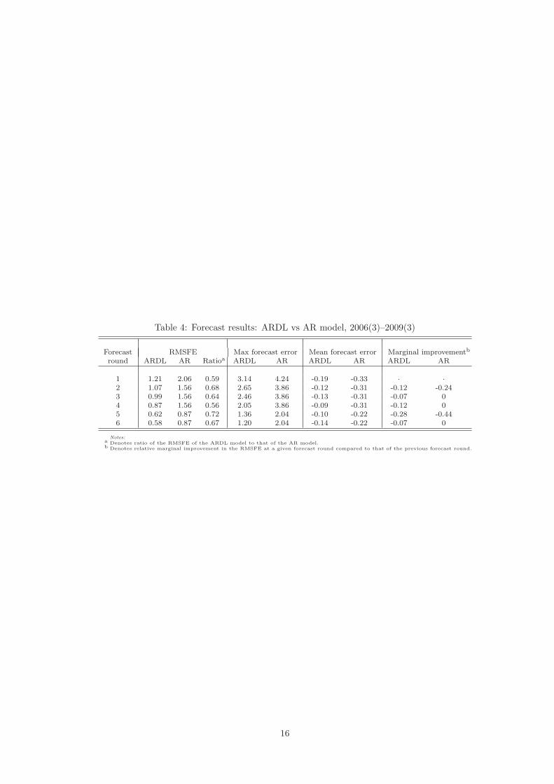
observed forecast errors are reported in Table 4 for the whole forecast sample, 2006(3)–2009(3). As seen, for
all forecast rounds, the model with the KOF Barometer yields a sizable improvement in forecast accuracy
over that reported for the univariate model. In fact, depending on a forecast round, the corresponding ratio
2Bayesian Model Averaging was carried out using the BMA package for R. Estimation of model parameters was carried outusing the MCMCpack package for R. All optional parameters for these two packages were left at their default values. Themaximum ratio of 20 for excluding models in Occam’s window has been used.
3A rather small number of models selected into the Occam’s window at the first forecast round e.g. compared to that forthe second forecast round can be explained by the fact that the forecast model employed for the first round is smaller than thatemployed for the second forecast round. The former model has only three own lags of the dependent variable Yt−3, Yt−4, Yt−5
whereas the other model has four lags—Yt−2, Yt−3, Yt−4, Yt−5, reflecting the availability of GDP data in real time, see Section4 and Table 1 for model specification and timing setup.
7
of the RMSFE of the ARDL model to that of the AR model varies between 0.56 and 0.72, implying an
improvement in forecast accuracy up to 44% in terms of RMSFE. It is also worthwhile mentioning that the
corresponding ratio for the earliest forecast round is solid 0.59, implying that substantial gains in forecast
precision can be achieved by using the model with the KOF Barometer as early as seven months before
the official release of GDP data. As expected, we observe further increase in forecast accuracy with every
forecast round as new information in terms of both GDP and the KOF Barometer values is incorporated in
every sequential forecast round. Thus, for the ARDL model the RMSFE falls from 1.21 reported for the first
forecast round to 0.58 in the last sixth forecast round. For the univariate AR model the corresponding values
of the RMSFE are 2.06 and 0.87, respectively. The model with the KOF Barometer produces also lower
maximum forecast error than that observed for the AR model and the forecasts of the former model appear
to be less biased than those of the latter model, although we observe a tendency of both models to overpredict
actual GDP growth rates. The forecasts of both the ARDL and AR models along with the corresponding
95% predictive intervals as well as the actual realizations of the real GDP quarterly year-on-year growth
rates are reported in Figures 1–6 for each forecast round.
The information reported in Table 4 also allows us to address the second question at which forecast round
the largest improvement in forecast accuracy is achieved. The column labeled as “Marginal improvement”
reports the relative reduction in RMSFE at a given forecast round compared to the previous forecast round.
Unsurprisingly, for the AR model we observe that reduction in RMSFE only occurs at the second and
fifth forecast rounds when, according to Table 1, an update of the GDP takes place. On the contrary,
for the ARDL model we observe reduction in RMSFE at each sequential forecast round, indicating that
incorporation of more recent values of the KOF Barometer (as well as of the GDP data) into the forecasting
equation results in gradual improvement in forecast accuracy. The largest marginal reduction in relative
RMSFE by 28% and 44% for both ARDL and AR models, respectively, occurs at the fifth forecast round,
i.e., about three months before an official release.
Finally, in order to address the third question on whether forecasting ability of the model with the
KOF Barometer has been changed during the current crisis compared to that observed in the pre-crisis
period. The relevant information is presented in Table 5 where we report RMSFE computed over the rolling
window of eight quarters rather than for the whole forecast period as displayed in Table 4 above. Several
observations can be made. First, similarly to the results observed for the whole forecast period, for a
given rolling forecast window we observe a steady increase in forecast accuracy with each forecast round
as more timely information is incorporated into forecasting equation; this equally refers to the ARDL as
well as the univariate AR model. Secondly, for the first four forecast rounds both for the ARDL and AR
models we observe a sharp deterioration in forecast accuracy starting from the rolling window 2007(1)–
2008(4) comparted to that observed for two previous rolling windows 2006(3)–2008(2) and 2006(4)–2008(3).
A further decrease in forecasting accuracy takes place for the next rolling window 2007(2)–2009(1). The
associated deterioration in forecast accuracy could be explained by relatively large forecast errors in quarters
2008(4) and 2009(1) as reflected in Figures 1–6. For the last two rolling windows for these four forecast rounds
the magnitude of RMSFE largerly remains stabile. Thirdly, for the last two forecast rounds for the ARDL
8
model we observe increase in RMSFE starting from the rolling window 2007(1)–2008(4) which stabilizes
at the window 2007(3)–2009(2). The evolution of RMSFE for each rolling window and forecast round is
graphically summarized in Figure 7. All in all, we can conclude that the magnitude of RMSFE observed for
the pre-crisis period has increased about two times compared to the period that also includes the current
crisis. However, this increase in RMSFE took place proportionally both for the ARDL and AR models such
that the ratio of RMSFE of these two models has been affected to a much smaller degree and depending on
evaluation window and forecast round takes values in the interval from 0.48 till 0.74 as shown in the lower
panel of Table 5. These values of the relative RMSFE are compatible with those observed for the whole
forecast period reported in Table 4.
6 Conclusion
In this paper we investigate whether the leading-indicator model based on the KOF Barometer which is
regularly published by the KOF Swiss Economic Institute on a monthly basis has any predictive power that
can be used for short-term forecasting of year-on-year quarterly real GDP growth rates in Switzerland well
ahead of the official data release by the Swiss State Secretariat for Economic Affairs (Seco). The forecasting
accuracy of the model with the KOF Barometer has been compared to a benchmark univariate autoregressive
model. Since the KOF Barometer is based on the business tendency surveys collected at the KOF, we also
investigate a more general question whether surveys, that are based on qualitative or “soft” data, are useful
for a quantitative short-run prediction of the so-called “hard” data. To this end, we produced a sequence
of forecasts for every quarter during the forecast sample from 2006(3) until 2009(3). We start with the
first forecast made about seven months ahead of GDP release by Seco, followed by the second forecast that
precedes GDP release by six months, etc., till the final sixth forecast made about two months ahead of the
first official GDP estimate. The important feature of our forecasting exercise is that at every forecast vintage
we employ the real-time data set that could have been available to a forecaster at the respective time in the
past. The real-time data set constructed for this purpose includes all real-time vintages of GDP data as well
as of the KOF Barometer.
Our main findings are as follows. First, the model with the KOF Barometer provides a substantial
improvement in forecast accuracy over the benchmark model as far as seven months ahead of the official
data release. Second, at every subsequent forecast round we observe increase in forecast accuracy as reflected
in steadily declining values of RMSFE criterion. The value of RMSFE for a model with the KOF Barometer
decreases from 1.21 achieved at the first forecast round till 0.58—at the last sixth forecast round. This has
to be compared to the corresponding values attained by the autoregressive model: 2.06 and 0.87, for the first
and sixth forecast rounds, respectively. The largest increase in forecast accuracy, however, is achieved at the
fifth forecast round; i.e., about three months ahead of an official data release. Third, during the period of
current crisis we find that the forecasting ability of the model with a leading indicator has deteriorated in
absolute value. Using the rolling window for computation of RMSFE, we find that for the leading-indicator
model inclusion of the quarters when the current crisis has been unfolding resulted in twice as large values of
9
RMSFE compared to that reported for the pre-crisis period. At the same time, we would like to emphasize
that forecast accuracy produced by the benchmark model has also deteriorated to a similar degree such that
in relative terms the forecasting performance of the model with the KOF Barometer remained relatively
unaffected by recent economic crisis.
All in all, based on the reported results of our forecast exercise the KOF Barometer possesses a definite
predictive content that can be used for early forecasts as well as nowcasts of the GDP growth rates up to
seven months prior to an official release.
References
Abberger, K. (2007). Forecasting quarter-on-quarter changes of German GDP with monthly business ten-
dency survey results. Ifo Working paper 40, Ifo Institute for Economic Research at the University of
Munich.
Balke, N. S. and D. Petersen (2002). How well does the Beige Book reflect economic activity? Evaluating
qualitative information quantitatively. Journal of Money, Credit and Banking 34 (1), 114–136.
Bergstrom, R. (1995). The relationship between manufacturing production and different business survey
series in Sweden 1968-1992. International Journal of Forecasting 11 (3), 379–393.
Croushore, D. (2005). Do consumer-confidence indexes help forecast consumer spending in real time? The
North American Journal of Economics and Finance 16 (3), 435–450.
Diebold, F. X. and G. D. Rudebusch (1991). Forecasting output with the composite leading index : A
real-time analysis. Journal of the American Statistical Association 86 (415), 603–610.
Etter, R. and M. Graff (2003). Estimating and forecasting production and orders in manufacturing industry
from business survey data: Evidence from Switzerland, 1990-2003. Swiss Journal of Economics and
Statistics 139 (4), 507–553.
Golinelli, R. and G. Parigi (2008). Real-time squared: A real-time data set for real-time GDP forecasting.
International Journal of Forecasting 24 (3), 368–385.
Graff, M. (2006). Ein multisektoraler Sammelindikator fur die Schweizer Konjunktur. Schweizerische
Zeitschrift fur Volkswirtschaft und Statistik 142, 529–577.
Graff, M. (2009). Does a multi-sectoral design improve indicator-based forecasts of the GDP growth rate?
Evidence for Switzerland. Applied Economics , forthcoming.
Graff, M. and R. Etter (2004). Coincident and leading indicators of manufacturing industry: Sales, produc-
tion, orders and inventories in Switzerland. Journal of Business Cycle Measurement and Analysis 1 (1),
109–113.
10
Hanssens, D. M. and P. M. Vanden Abeele (1987). A time-series study of the formation and predictive
performance of EEC production survey expectations. Journal of Business & Economic Statistics 5 (4),
507–519.
Hansson, J., P. Jansson, and M. Lof (2005). Business survey data: Do they help in forecasting GDP growth?
International Journal of Forecasting 21 (2), 377–389.
Hendry, D. F. and H.-M. Krolzig (2001). Automatic Econometric Model Selection Using PcGets. London:
Timberlake Consultants Ltd.
Hoeting, J., D. M. A. Raftery, and C. Volinsky (1999). Bayesian model averaging: A tutorial. Statistical
Science 14, 382–401.
Jacobs, J. P. and J.-E. Sturm (2009). The information content of KOF indicators on Swiss current account
data revisions. Journal of Business Cycle Measurement and Analysis 2008 (2), 35–57.
Kauppi, E., J. Lassila, and T. Terasvirta (1996). Short-term forecasting of industrial production with
business survey data: Experience from Finland’s great depression 1990-1993. International Journal of
Forecasting 12 (3), 373–381.
Koberl, E. and S. M. Lein (2008). The NAICU and the Phillips Curve - An approach based on micro data.
Working paper 08-211, KOF Swiss Economic Institute, ETH Zurich.
Lemmens, A., C. Croux, and M. G. Dekimpe (2005). On the predictive content of production surveys: A
pan-European study. International Journal of Forecasting 21 (2), 363–375.
Lindstrom, T. (2000). Qualitative survey responses and production over the business cycle. Working Paper
Series 116, Sveriges Riksbank (Central Bank of Sweden).
Madigan, D. and A. E. Raftery (1994). Model selection and accounting for model uncertainty in graphical
models using Occam’s window. Journal of the American Statistical Association 89, 1535–1546.
Markku, R. and T. Timo (1993). Business survey data in forecasting the output of Swedish and Finnish
metal and engineering industries: A Kalman filter approach. Journal of Forecasting 12 (3-4), 255–271.
Muller, C. and E. Koberl (2008a). Business cycle measurement: A semantic identification approach using
firm level data. Working paper 08-212, KOF Swiss Economic Institute, ETH Zurich.
Muller, C. and E. Koberl (2008b). The speed of adjustment to demand shocks: A Markov-chain measurement
using micro panel data. Working paper 07-170, KOF Swiss Economic Institute, ETH Zurich.
Muller, C., A. Wirz, and N. Sydow (2008). A note on the Carlson-Parkin method of quantifying qualitative
data. Working paper 07-168, KOF Swiss Economic Institute, ETH Zurich.
Okun, A. M. (1962). The predictive value of surveys of business intentions. The American Economic
Review 52 (2), 218–225.
11
Oller, L.-E. (1990). Forecasting the business cycle using survey data. International Journal of Forecast-
ing 6 (4), 453–461.
Oller, L.-E. and C. Tallbom (1996). Smooth and timely business cycle indicators for noisy Swedish data.
International Journal of Forecasting 12 (3), 389–402.
Raftery, A. E. (1995). Bayesian model selection in social research. Sociological Methodology 25, 111–163.
Rupprecht, S. M. (2008). When do firms adjust prices? Evidence from micro panel data. Working paper
07-160, KOF Swiss Economic Institute, ETH Zurich.
Schenker, R. (2008). Comparing quantitative and qualitative survey data. Working paper 07-169, KOF
Swiss Economic Institute, ETH Zurich.
Stock, J. H. and M. W. Watson (1988). A probability model of the coincident economic indicators. NBER
Working Papers 2772, National Bureau of Economic Research, Inc.
Stock, J. H. and M. W. Watson (2002). Macroeconomic forecasting using diffusion indexes. Journal of
Business and Economic Statistics 20 (2), 147–162.
Terasvirta, T. (1986). Model selection using business survey data: Forecasting the output of the Finnish
metal and engineering industries. International Journal of Forecasting 2 (2), 191 – 200.
Zarnowitz, V. (1973). A review of cyclical indicators for the United States: Preliminary results. NBER
Working Papers 0006, National Bureau of Economic Research, Inc.
12
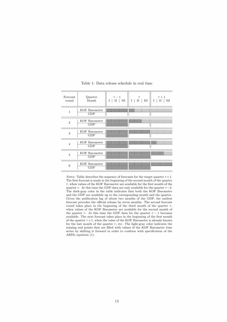
Table 1: Data release schedule in real time
Forecast Quarter τ − 1 τ τ + 1round Month I II III I II III I II III
1KOF Barometer
GDP
2KOF Barometer
GDP
3KOF Barometer
GDP
4KOF Barometer
GDP
5KOF Barometer
GDP
6KOF Barometer
GDP
Notes: Table describes the sequence of forecasts for the target quarter τ+1.The first forecast is made in the beginning of the second month of the quarterτ , when values of the KOF Barometer are available for the first month of thequarter τ . At this time the GDP data are only available for the quarter τ−2.The dark-gray color in the table indicates that both the KOF Barometerand the GDP are available up to the corresponding month and the quarter.Given the publication lag of about two months of the GDP, the earliestforecast precedes the official release by seven months. The second forecastround takes place in the beginning of the third month of the quarter τ ,when values of the KOF Barometer are available for the second month ofthe quarter τ . At this time the GDP data for the quarter τ − 1 becomesavailable. The next forecast takes place in the beginning of the first monthof the quarter τ+1, when the value of the KOF Barometer is already knownfor the last month of the quarter τ , etc. The light-gray color indicates themissing end points that are filled with values of the KOF Barometer timeseries by shifting it forward in order to conform with specification of theARDL equation (1).
13
Table 2: Results of the BMA procedure (symmetric Occam’s window), 1993(4)–2009(2), Forecast round 6
Notes:a Denotes inclusion frequency of each regressor in the models retained in the symmetric Occam’s window, see equation (1).b,c EV and SD stand for “Expected Value” and “Standard Deviation” of the posterior distribution of the model parameters.
14
Table 3: Summary of the BMA procedure (symmetric Occam’s window), all forecast rounds
Forecast round 1 Forecast round 2Forecast Number of Posterior probabilityb Inclusion Number of Posterior probability Inclusionquarter modelsa max min frequency (Xt)c models max min frequency (Xt)
Forecast round 3 Forecast round 4Number of Posterior probability Inclusion Number of Posterior probability Inclusionmodels max min frequency (Xt) models max min frequency (Xt)
Forecast round 5 Forecast round 6Number of Posterior probability Inclusion Number of Posterior probability Inclusionmodels max min frequency (Xt) models max min frequency (Xt)
Notes:a Denotes number of models selected in symmetric Occam’s window.b Denotes maximum and minimum of assigned posterior probabilities of the models retained in the symmetric Occam’s window.c Denotes inclusion frequency of the contemporaneous values of the KOF Barometer Xt in the models retained in the symmetric Occam’s window, see
equation (1).
15
Table 4: Forecast results: ARDL vs AR model, 2006(3)–2009(3)
Forecast RMSFE Max forecast error Mean forecast error Marginal improvementb
Notes:a Denotes ratio of the RMSFE of the ARDL model to that of the AR model.b Denotes relative marginal improvement in the RMSFE at a given forecast round compared to that of the previous forecast round.
16
Table 5: Forecast results: ARDL vs AR model, rolling forecast sample
Table entries are RMSFE reported for the rolling window for each forecast round for the ARLDand AR models in the upper and middle panels, respectively. The ratio of RMSFE of the ARDLto that of the AR model is reported in the lower panel.
17
2007 2008 2009
−2.5
0.0
2.5
5.0
GDP yoy 95%
ARDL 95%
2007 2008 2009
−2.5
0.0
2.5
5.0
GDP yoy 95%
AR 95%
Figure 1: Forecast round 1: (Upper panel) Forecasts of the ARDL model with a 95% predictive interval,Actual values of the quarterly year-on-year real GDP growth rates (first release); (Lower panel) Forecasts ofthe AR model with a 95% predictive interval, Actual values of the quarterly year-on-year real GDP growthrates (first release)
18
2007 2008 2009
−5.0
−2.5
0.0
2.5
5.0
GDP yoy 95%
ARDL 95%
2007 2008 2009
−2.5
0.0
2.5
5.0
GDP yoy 95%
AR 95%
Figure 2: Forecast round 2: (Upper panel) Forecasts of the ARDL model with a 95% predictive interval,Actual values of the quarterly year-on-year real GDP growth rates (first release); (Lower panel) Forecasts ofthe AR model with a 95% predictive interval, Actual values of the quarterly year-on-year real GDP growthrates (first release)
19
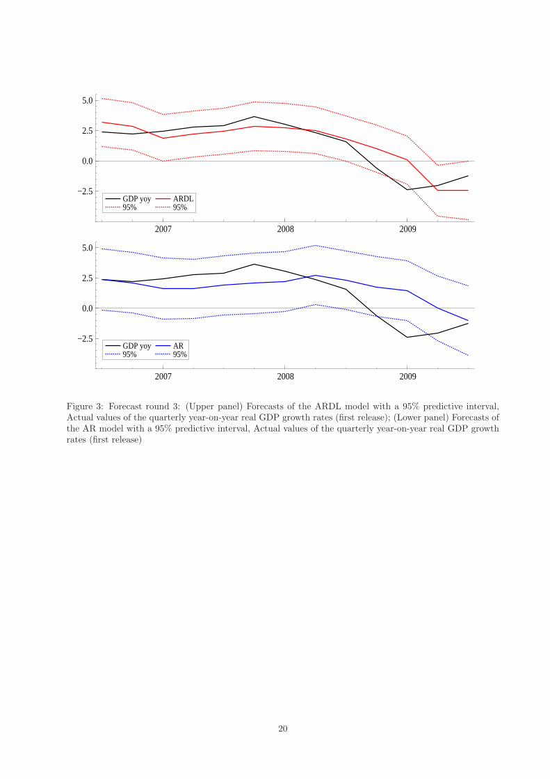
2007 2008 2009
−2.5
0.0
2.5
5.0
GDP yoy 95%
ARDL 95%
2007 2008 2009
−2.5
0.0
2.5
5.0
GDP yoy 95%
AR 95%
Figure 3: Forecast round 3: (Upper panel) Forecasts of the ARDL model with a 95% predictive interval,Actual values of the quarterly year-on-year real GDP growth rates (first release); (Lower panel) Forecasts ofthe AR model with a 95% predictive interval, Actual values of the quarterly year-on-year real GDP growthrates (first release)
20
2007 2008 2009
−2.5
0.0
2.5
5.0
GDP yoy 95%
ARDL 95%
2007 2008 2009
−2.5
0.0
2.5
5.0
GDP yoy 95%
AR 95%
Figure 4: Forecast round 4: (Upper panel) Forecasts of the ARDL model with a 95% predictive interval,Actual values of the quarterly year-on-year real GDP growth rates (first release); (Lower panel) Forecasts ofthe AR model with a 95% predictive interval, Actual values of the quarterly year-on-year real GDP growthrates (first release)
21
2007 2008 2009−5.0
−2.5
0.0
2.5
5.0
GDP yoy 95%
ARDL 95%
2007 2008 2009−5.0
−2.5
0.0
2.5
5.0
GDP yoy 95%
AR 95%
Figure 5: Forecast round 5: (Upper panel) Forecasts of the ARDL model with a 95% predictive interval,Actual values of the quarterly year-on-year real GDP growth rates (first release); (Lower panel) Forecasts ofthe AR model with a 95% predictive interval, Actual values of the quarterly year-on-year real GDP growthrates (first release)
22
2007 2008 2009−5.0
−2.5
0.0
2.5
5.0
GDP yoy 95%
ARDL 95%
2007 2008 2009−5.0
−2.5
0.0
2.5
5.0
GDP yoy 95%
AR 95%
Figure 6: Forecast round 6: (Upper panel) Forecasts of the ARDL model with a 95% predictive interval,Actual values of the quarterly year-on-year real GDP growth rates (first release); (Lower panel) Forecasts ofthe AR model with a 95% predictive interval, Actual values of the quarterly year-on-year real GDP growthrates (first release)