Page 1
Assessing Risk-based Policies for Pretrial Release and
Split Sentencing in Los Angeles County Jails
Mericcan Usta∗, Lawrence M. Wein†
July 23, 2015
∗Management Science & Engineering Department, Stanford University, Stanford, CA 94305,
[email protected] †Graduate School of Business, Stanford University, Stanford, CA 94305, [email protected]
1
Page 2
Abstract
Court-mandated downsizing of the CA prison system has led to a redistribution of
detainees from prisons to CA county jails, and subsequent jail overcrowding. Using data
that is representative of the LA County jail system, we build a mathematical model
that tracks the flow of individuals during arraignment, pretrial release or detention,
case disposition, jail sentence, and possible recidivism during pretrial release, after a
failure to appear in court, during non-felony probation and during felony supervision.
We assess 64 joint pretrial release and split-sentencing (where low-level felon sentences
are split between jail time and mandatory supervision) policies that are based on the
type of charge (felony or non-felony) and the risk category as determined by the CA
Static Risk Assessment tool, and compare their performance to that of the policy LA
County used in early 2014, before split sentencing was in use. In our model, policies
that offer split sentences to all low-level felons optimize the key tradeoff between public
safety and jail congestion by, e.g., simultaneously reducing the rearrest rate by 7%
and the mean jail population by 20% relative to the policy LA County used in 2014.
The effectiveness of split sentencing is due to two facts: (i) convicted felony offenders
comprised ≈ 45% of LA County’s jail population in 2014, and (ii) compared to pretrial
release, split sentencing exposes offenders to much less time under recidivism risk per
saved jail day.
2
Page 3
To mitigate severe prison overcrowding, the U.S. Supreme Court (Brown v. Plata,
2011) forced the state of California (CA) to reduce its prison population by 25% within
two years. In response, CA passed the Public Safety Realignment Act (Assembly Bill 109,
often referred to as realignment), which called for low-level (i.e., non-serious, non-violent,
non-sex-related) felonies and state parole violations to be punishable by incarceration in
county jails rather than state prisons. Although realignment has successfully reduced the
state prison population, it has caused a significant increase in the CA jail population: of the
58 CA counties, 19 (including LA County) have court-ordered jail population caps [1] (some
counties rent jail space from other counties), and 21 counties are receiving CA state funds
to add > 10k additional jail beds [2].
CA counties have two primary options for reducing jail overcrowding in the short run.
They can offer pretrial release to defendants, in the hope that these defendants appear
in court and do not recidivate (i.e., commit another crime) prior to case disposition. In
addition, Assembly Bill 1468 requires that – unless the court finds it is not in the interest
of justice – as of January 1, 2015 low-level felony sentences be split between jail time and
mandatory supervision. To aid in these decisions, correctional systems throughout the U.S.
employ risk-based tools that use a defendant’s demographic data and criminal history to
predict the likelihood of recidivism and of appearing in court. These tools are moderately
predictive, achieving an area under the curve of the receiver operating characteristic curve
of ≈ 0.7 [3], meaning, e.g., that the probability a three-year recidivist has a higher risk score
than a three-year non-recidivist is 0.7.
To investigate jail management under these circumstances, we build a simulation model
that tracks the flow of inmates over time in LA County jails, which is the world’s largest
jail system. In our model, individuals arrive for arraignment as one of six types, according
to whether their current charge is a felony or non-felony, and whether their risk category is
low, medium or high in the California Static Risk Assessment (CSRA) tool [4], which is one
3
Page 4
of the risk tools used in CA. Using a queueing network model for process flow and statis-
tical models for risk-based recidivism and failure to appear in court, we follow individuals
through arraignment, pretrial detention or release, case disposition and jail sentence, as well
as recidivism that may occur during pretrial release, after a failure to appear in court, during
regular probation for non-felonies, and during supervision of a split sentence for felonies. We
assess 64 joint pretrial release and split-sentencing policies that are risk-based, and compare
them to the status quo policy that LA County was using in 2014; despite the passage of
Assembly Bill 1468, LA County used split sentencing only sparingly in early 2015 (Fig. 6 in
[5]). Our goal is to identify policies that optimize the tradeoff between public safety – as
measured by the annual rearrest rate of anyone on pretrial release, after a failure to appear
in court, on regular probation or on supervision during a split sentence – and jail congestion,
as measured by the mean jail population or the mean amount of jail overcrowding (i.e.,
population in excess of jail capacity).
Methods
The model is depicted in Fig. 1, the policies are described in Tables 1-2, and a list
of model parameters and their values are given in Tables 3-4. Details of the parameter
estimation procedure appear in the Supporting Information (SI).
Process Flow. New inmates arrive to the county jail system according to a renewal process,
where the time between consecutive arrivals has an Erlang distribution. The county jail has
a fixed capacity, but we assume that some detainees are held in a different jail (e.g., in
another county or at a U.S. Immigration and Customs Enforcement facility) if the current
jail population exceeds its capacity. The arriving defendants are randomly assigned to one of
six types, according to a combination of their charge (non-felony or felony, where the former
consists of misdemeanors and lesser charges) and their CSRA risk category (low, medium
or high), where the risk category and charge probabilities are assumed to be statistically
independent. After a short random delay, defendants undergo arraignment, during which
4
Page 5
the first of two key decisions is made: based on a defendant’s charge-risk type, either release
the defendant until case disposition (i.e., pretrial release) or hold him (we adopt the male
gender throughout) in custody until case disposition (our model does not incorporate the
many arrests that do not result in arraignment [9]).
The time delay from arraignment until case disposition is random and depends upon a
defendant’s charge (non-felony vs. felony) and pretrial release vs. custody status, but not on
his CSRA risk. Defendants on pretrial release possess two competing random times: the time
from arraignment to recidivism (which is based on a statistical model that depends on his
CSRA risk but not on his charge, and which can be infinite) and the time from arraignment
until case disposition. If the former time is shorter than the latter time, then the defendant
recidivates before case disposition; his recidivism charge is assumed to be the same as his
original charge and his risk is unchanged (note that CSRA and some other risk tools do
not use the current charge as a predictive variable due to its lack of predictiveness [4]).
The recidivating defendant re-enters the jail and waits for a new arraignment, and the new
pretrial release vs. custody decision takes into account his recent recidivism, as described
later.
If the time from arraignment to case disposition is shorter than the time from arraign-
ment to recidivism for a defendant on pretrial release, he does not recidivate before case
disposition. In this case, we assume that the likelihood of failing to appear in court for case
disposition depends on the defendant’s risk category but not on his charge type. If he does
not appear in court, then his time from arraignment to recidivism remains active, and he
may recidivate at a later time, at which point he is treated in the same way as those who
recidivate before case disposition.
Case disposition for non-felonies has three possible outcomes, with probabilities that
depend upon the pretrial release vs. custody status: acquittal/dismissal (and exit from the
system), probation, or a jail term that also includes a probation component. The random
5
Page 6
length of probation is statistically identical, whether or not it is preceded by a jail term.
Similarly, felony cases have four possible dispositions with probabilities that depend upon
the release vs. custody status: acquittal/dismissal, probation, jail (without probation), and
prison, where those going to prison exit our model. The length of the post-sentence jail
term depends on both the charge (non-felony vs. felony) and the pretrial status (release
vs. custody). Later we discuss the key assumption that the time from arraignment to case
disposition, the court outcome and the length of the post-sentencing jail term depend on
whether the offender is released or detained prior to trial.
The second of our two policy decisions is made during case disposition of felonies:
whether or not – depending upon the risk category of the offender – to offer split sentences
for felonies (all felons in our model are low-level felons that are eligible for split sentencing).
Felons receiving a split sentence spend the first half of their post-sentence jail term in jail,
and spend the second half out on mandatory community supervision, where the 50-50 split
is based on recent reports from CA counties [5, 17, 18]. Finally, offenders on probation or
supervision are assumed to recidivate according to the same statistical model as offenders on
pretrial release, but – in contrast to recidivists on pretrial release, who are typically released
for a shorter amount of time – they are assigned a new charge at random (although their
risk does not change) before returning for re-arraignment, and the new pretrial release vs.
custody decision takes into account his recent recidivism, as described later.
Policies. Our pretrial release decisions are based on an offender’s charge-risk type, and the
split-sentencing decisions for felons are based on their risk category. We restrict ourselves
to policies that are independent of the current number of inmates in jail and are monotonic
in risk; i.e., if a certain offender is offered pretrial release then all offenders with the same
charge and with the same or lower risk is also offered pretrial release, and if a felon is offered
a split sentence then all felons with the same or lower risk is also offered a split sentence.
Hence, because there are four options for each risk category (offering the option to no one,
6
Page 7
to only low-risk individuals, to low- and medium-risk individuals, or to everyone) and three
decisions (pretrial release for non-felonies, pretrial release for felonies, split-sentencing for
felonies), we consider 43 = 64 policies that correspond to all combinations of one option
from each of the three columns in Table 1.
In addition, we consider a policy that represents the status quo in LA County in early
2014. This policy does not offer split-sentencing to any offenders because LA County’s use
of split sentencing was < 1% during June 2013 - May 2014 (Fig. 6 in [5]). The probability
of pretrial release in LA County depended upon the charge-risk type (Table 2), and these
probabilities are estimated using data in [9, 19, 20] (§1 in SI).
The decisions in Tables 1 and 2 apply only to new arrivals. If an offender recidivates
during pretrial release, then he is detained after rearraignment under the 64 policies in
Table 1 and the status quo policy. If an offender recidivates during probation or supervision,
then he is offered pretrial release with probability 0.2 if his recidivism charge is a non-felony
and with probability 0.1 if his recidivism charge is a felony, independent of an offender’s risk
category (§2 in SI); these pretrial release probabilities are based on financial conditions (i.e.,
defendants are able to post bail or a bond, which is rarely denied in LA County) rather than
risk, and are applied to all 65 policies.
Performance Measures. Our key tradeoff is between public safety and jail congestion.
We measure public safety by the annual number of jailed rearrests of (i.e., recidivist crimes
by) anyone on pretrial release, probation or supervision, or after a failure to appear in court.
We measure jail congestion in two ways: by the mean size of the jail population over the
length of the simulation, or by the mean amount of overcrowding, which is the mean of the
number of inmates in excess of the county jail capacity at each point in time.
Parameter Estimation.
Jail Capacity. The jail capacity of 19,000 is approximately halfway between the functional
bed capacity (set at 90% of capacity to allow for seasonal fluctuations and the need to
7
Page 8
separate special-need and high-risk inmates) of LA County projection options A and C
(19,530) and option B (18,630) in Table 14 of [6]. This estimate is also consistent with the
rated (by the Board of State and Community Corrections) capacity with the inclusion of
fire camps of 19,474 (page 4 of [7]) minus the ≈ 500 prison inmates and transfers that are
housed in jail.
Interarrival Times. The interarrival time distribution is derived from arraignment data (e.g.,
[8]) during 2008-2012 in LA County (§3 in SI).
Time Delay From Arrest To Arraignment. The parameters for the time delay from arrest
to arraignment are derived from 2008 data from LA County [9] via maximum likelihood
estimation (§4 in SI).
Charge Proportion. Using the “Cases Matched from PIMS to AJIS” column in Table 3 of [9],
we estimate that the proportion of defendants who have a felony charge is 49,549/112,201=0.442,
and the proportion who have a non-felony charge is 0.558.
Risk Tool. We initially considered two risk tools, Correctional Offender Management Pro-
filing for Alternative Sanctions (COMPAS) [21] and CSRA [4], that have been used by CA
correctional agencies and externally validated (albeit on pre-alignment state parole popu-
lations rather than post-alignment jail populations). The main advantage of COMPAS is
that it has a finer granularity of risk (10 risk categories) than CSRA (three risk categories).
However, we chose to adopt CSRA in this study because its validation study for recidivism
[10] has finer temporal granularity and less right-censoring (recidivism at 1, 2 and 3 years
for 110,313 parolees) than the COMPAS validation study [22] (recidivism at 2 years for a
sample of 24,418 parolees), both of which are required to develop a reliable statistical model
for time to recidivism. Here, recidivism refers to an arrest and return to custody, which
is the most relevant definition for jail capacity and cost [21]. However, because we could
not locate any studies that calibrated the CSRA risk tool to failure-to-appear data, we use
COMPAS (after aggregating its 10 risk categories into CSRA’s three risk categories, as in
8
Page 9
page 20 in [11]) to estimate the risk-based likelihood of failing to appear in court.
Risk Proportion. We use the risk category breakdown of the 110,313 parolees in Table 15 of
[10] to get the proportions in Table 3.
Time to Recidivism. Using maximum likelihood estimation, we fit five models (§5 in SI) to
the raw data in Table 15 of [10] (recidivism within 1 year, 2 years and 3 years for each of three
risk categories): a lognormal model (where the mean parameter is an affine function of the
risk score), a split lognormal model (where a proportion of the population – independent of
risk – never recidivate [23] and the others recidivate according to a lognormal distribution),
a split lognormal model with heteroskedasticity (the standard deviation parameter is also an
affine function of the risk score), a proportional hazards model [24], and a split proportional
hazards model. The split lognormal model with heteroskedasticity provides the best fit (§5
in SI). The lognormal distribution exhibits a unimodal hazard rate, which captures a brief
period of desistance followed by a peak incidence of recidivism and a slowdown thereafter
(Fig. 1 in SI). The split improves the empirical fit, as seen in earlier studies (e.g., [25]).
Failure to Appear. We use a study that validates the COMPAS tool using 18 months of data
from Broward County’s (FL) jail system [11] to estimate the failure-to-appear probabilities
in Table 3 (§6 in SI).
Time from Arraignment to Disposition. We use maximum likelihood estimation to fit log-
normal and gamma distributions to arrest-to-disposition time data from [9] (§7 in SI).
Case Disposition Probabilities. The 14 case disposition probabilities in Table 4 are estimated
in §8 in SI using Bayes rule and data in Table 4 of [9], pages 57 and 129 of [9] and Table 1
in [13], and odds ratio estimates on page 10 of [12].
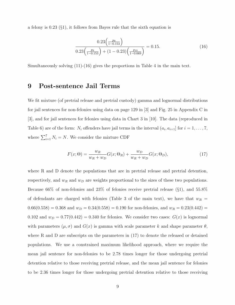
Post-sentence Jail Terms. We fit mixture (of pretrial release and pretrial custody) lognormal
and gamma distributions for jail sentences using non-felony data on page 129 in [9] and
Fig. 25 in Appendix C in [9], and felony data in Chart 3 in [14] (§9 in SI).
Length of Probation. Although typical non-felony probation duration is widely reported by
9
Page 10
criminal law offices as one year (with no minimum and a maximum of three years) [15] and
typical felony probation duration is given as three years (with a minimum of one year and a
maximum of five years) [16], we could not locate data on their distribution. Consequently, we
chose triangular distributions with these ranges and with modes as their typical durations.
Results
For all reported results, we simulate 1000 runs of 2000 days each – collecting statistics
only after the 900th day – and report on the mean of the 1000 replications.
Model Validation of Jail Population and Composition. We begin by simulating
the status quo policy (Table 2) and find that the total jail population, the composition of
felons vs. non-felons and sentenced vs. non-sentenced, and the amount of overcrowding are
generally consistent with reported values for LA County (Table 5).
A Simple Metric. To provide a framework for interpreting our main results, we introduce
a simple metric that quantifies the tradeoff involved in the three components of our policies
(Table 1): pretrial release for non-felons, pretrial release for felons, and split sentences for
felons. Each decision entails releasing a defendant or offender for an amount of time, and
– in exchange for the increased recidivism risk - we are reducing the jail population by one
person for a possibly different amount of time. Our metric, which we call the risk ratio, is the
amount of time that a defendant or offender is released divided by the number of jail-days
saved, where both of these quantities are conditioned on the person not recidivating. By our
modeling assumptions, this ratio is 1.0 for split sentencing because the number of jail-days
saved is the same as the number of days on supervision. In contrast, calculating the means
of the gamma and lognormal distributions specified in Table 4, we see (Table 6) that the
pretrial release of a non-felon achieves an average reduction of 8 jail-days in exchange for a
recidivism risk over an average of 128 days (for a ratio of 16) and the pretrial release of a
felon achieves an average reduction of 53 jail-days in exchange for a recidivism risk over an
average of 191 days (for a ratio of 3.6). Although this ratio is crude – it fails to account for
10
Page 11
the reduction in jail-days saved due to recidivism on supervision or before case disposition,
the larger reduction in jail-days saved if a defendant fails to appear in court, and the future
increase in jail population after a recidivist is rearraigned. Nonetheless, this ratio provides
a first-order quantification of the nature of these tradeoffs. This ratio reveals that – for a
specified risk category (low, medium or high) - split sentencing offers the most favorable
tradeoff, followed by the pretrial release for felons, with the pretrial release of non-felons
generating the least desirable tradeoff.
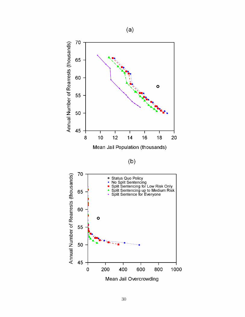
Main Results. In our numerical results, the mean jail overcrowding is a nondecreasing
function of the mean jail population; consequently, we focus most of our discussion on the
tradeoff between the annual rearrest rate and the mean jail population. Our main results
(Fig. 2a) show the performance of the status quo policy and four tradeoff curves, one for each
of the split-sentencing options in Table 1. Each of the four tradeoff curves connects up to 16
points, one for each of the 16 possible pretrial release policies in Table 1. The optimal pretrial
release policies for these four tradeoff curves are specified in Fig. 3, using the numbering
system in Table 1. In total, eight of the 64 policies are dominated by other policies that use
the same split-sentencing option (i.e., these other policies achieve simultaneous reductions
in rearrest rate and mean jail population) and do not appear in Fig. 3. Not surprisingly
(Table 5), the dominated policies favor the pretrial release of non-felons over felons; e.g., in
Fig. 3a, the two dominated pretrial release policies are (2,0) and (3,0), using the numbering
system in Table 1. For a given split-sentencing option, we connect these points to create
a tradeoff curve only for ease of visualization, and did not assess the performance of any
policies that randomize between different points on a tradeoff curve.
The main insight from Fig. 2a is the importance of offering split sentencing to high-
risk felons. The reduction in the performance measures between the tradeoff curve that
offers split sentencing to all felons and the tradeoff curve that offers split sentencing to only
low- and medium-risk felons is much larger than the reduction in the performance measures
11
Page 12
between the tradeoff curve offering split sentencing to only low- and medium-risk felons and
the tradeoff curve offering no split sentencing. This result is due to the low risk ratio of
split sentencing (Table 6), coupled with the facts that convicted felons make up a significant
portion of the jail population (Table 5) and the majority of them are high risk (Table 4).
Relative to the status quo policy, the tradeoff curve that provides split sentencing to all
felons achieves a 29% reduction in the jail population level at the same rearrest rate, or,
e.g., simultaneously reduces the jail population by 20% and the rearrest rate by 7%. The
suboptimality of the status quo policy relative to all four of these tradeoff curves stems from
the fact that the status quo policy is not purely risk-based (Table 2).
The four curves in Fig. 2a do not exhibit the strong convexities that would be associated
with increasing marginal risk at a higher release rate. The one exception is the near vertical
jump from (3,2) to (0,3) (Fig. 3), where a switch from pretrial releasing all non-felons and
some felons to pretrial releasing all felons and no non-felons leads to a very small reduction
in jail population but a significant increase in the rearrest rate.
The optimal tradeoff curve among all 64 policies is the lower-left envelope of the four
tradeoff curves, which consists of the entire leftmost (i.e., split sentencing for everyone) curve
and the bottom portions of the other three curves. The only scenario in which offering split
sentencing to all felons is not optimal is where it is deemed important to minimize the total
rearrest rate below 51.5k/yr (which is the lowest level achievable by any policy that offers
split sentencing to all felons). Comparing the lower endpoints of the two leftmost curves in
Fig. 2a, we see that disallowing split sentencing for high-risk felons while continuing to offer
split sentencing to other felons and pretrial release to everyone, the average annual rearrest
rate can be decreased by 2%, but the jail population increases by 14%; this change represents
a much less attractive tradeoff than when the total arrest rate is > 51.5k/yr. In contrast, if
the primary concern is with jail overcrowding rather than the mean jail population, then less
aggressive jail population reduction policies can be considered because many of the policies
12
Page 13
from Table 1 totally eliminate jail overcrowding (Fig. 2b; the analog of Fig. 3 for the jail
overcrowding metric appears in Fig. 2 in SI).
Despite the risk ratios in Table 6, it may not be practical to use a more aggressive
pretrial release policy for felonies than for non-felonies. Consequently, we restrict our con-
sideration of policies to those that treat felonies at least as strictly (with respect to pretrial
release) as non-felonies of the same risk category; i.e., we only allow pretrial release policies
(i,j) such that i≥j. The resulting tradeoff curves with this additional restriction appear in
Fig. 3 of SI, and are nearly linear.
Discussion
While LA County may be the most prominent example, many other counties in CA
[1, 2] and throughout the U.S. are struggling with overcrowding. Our model allows us to
assess how pretrial release and split-sentencing decisions impact the key tradeoff between
public safety and jail congestion. In our view, the study’s main contributions are in (i)
developing a mathematical model that captures the salient features of the problem and
provides a framework for quantifying the tradeoff between public safety and jail congestion,
(ii) introducing a simple metric - the risk ratio in Table 6 – that sheds light on the varying
amount of risk inherent in each type of decision in Table 1, (iii) identifying key data needs,
and (iv) highlighting key assumptions and issues. However, there are a number of limitations
to our study that need to be addressed before our main results can be directly applied. Hence,
before discussing our main results, we describe the limitations of the study, from a data and
a structural viewpoint.
Limitations. There are several shortcomings in the data. First, the survival model used
to determine the time to recidivism is the same, regardless of whether a person is out on
pretrial release, has failed to appear in court, is on probation after a non-felony, or is on
supervision during the latter part of a split sentence for a low-level felony. Moreover, the
recidivism model is calibrated using pre-alignment state parolee data, which is a different
13
Page 14
population than the post-alignment jail population that is the focus of our model. Because
many state prisoners and parolees became the responsibility of the county jail system during
realignment, it is possible that the pre-alignment parole population does not behave very
differently than the post-alignment jail population. But before our model can be applied to
a CA county jail system, the risk models commonly used in CA (e.g., CSRA and COMPAS)
need to be validated separately for the jail subpopulations that are on pretrial release, after
failure to appear in court, non-felony probation and low-level felony supervision.
On a similar note, we also estimate the risk profile of defendants entering arraignment
in our model from the risk profile of released state parolees during pre-alignment. Because
many offenders arraigned on non-felony charges have a felony background, this assumption
may not be as bold as it appears at first blush. Nonetheless, our model needs to use the
risk profile of the actual jail population before it can be reliably used. We also assume that
risk category and charge type are statistically independent, and this assumption should be
investigated, which requires separate risk distributions for non-felons and felons.
The only failure-to-appear data we found that is sufficiently detailed for our purposes
are from Broward County, FL [11], which may have a different defendant population than
LA County. The failure-to-appear probability in [11] is consistent with other estimates from
KY (page 2 in [29]) and a nationwide study of federal prisoners [12], although lower than a
0.4 estimate from a large urban center [30]. In addition, the data in [11] do not include the
time of each defendant’s case disposition, which prevents us from assessing (e.g., via logistic
regression) whether the likelihood of appearing in court is impacted by the arraignment-to-
disposition delay.
The CA jail system continues to be in flux due to the November 4, 2014 passage
of Proposition 47 (Safe Neighborhoods and Schools Act), which reclassifies several drug-
and theft-related offenses as non-felonies and allows for resentencing of previously convicted
felons. This change altered the composition and total population of CA jails, and the
14
Page 15
immediate reduction in jail population in November 2014 was largely counteracted by an
increase in time served for traditional jail inmates (pages 3-4 in [5]). Our model needs to
account for these recent changes before it can be used in CA.
A provocative aspect of our model – and indeed of the U.S. correctional system – is
that the time from arraignment to case disposition, the court outcomes and the length of
post-sentencing jail terms depend on whether the offender is released or held in custody prior
to trial. More specifically, the delays are shorter, the outcomes are more severe and the jail
terms are longer for those held in custody. These phenomena have been observed elsewhere
in the literature (§2b of [31]), even after controlling for prior convictions, the severity of the
current charge, and the strength of the evidence against the defendant [32]. However, we
assume that these structural differences, which can be seen by comparing the columns in
Table 4, hold regardless of the aggressiveness of the pretrial release policy (Table 1). As a
result, awarding a defendant pretrial release reduces the jail population in our model in three
ways: it keeps the offender out of jail before case disposition, it reduces the likelihood that
he is returned to jail at case disposition, and it reduces his jail time if he is returned to jail.
There may be some merit in this assumption (beyond the results in [31, 32]) because those on
pretrial release have a greater opportunity to impress jurors and judges (e.g., by appearing in
a socially acceptable attire instead of a jail uniform, maintaining a job and not recidivating)
and to provide a strong legal defense [31]. However, it is also likely that the pretrial release
decisions are based partially on data that are not included in our model; e.g., that judges
set higher bonds – leading to less likely pretrial release – when they view the probability of
acquittal as low [33], or when they incorporate retribution concerns (e.g., LA County does
not accept inmates with bail < $25k for non-felonies, and so courts set the bail ≥ $25k if they
want to guarantee detention [9]). To the extent that this is true, we may be overestimating
the benefit (in terms of a reduction in jail population and retribution) of pretrial release.
However, because our main result is that an aggressive split-sentencing policy is optimal,
15
Page 16
this assumption – by overstating the benefits of pretrial release – is conservative.
Another implicit set of assumptions is the model’s boundaries. While the correctional
system has many interacting parts [2], we consider several important aspects as exogenous.
One aspect is court processing capacity and prosecution behavior, both of which can delay
case disposition [31]. Note that by assuming exogenous delays until case disposition, we do
not capture the counterintuitive fact (implied by priority queueing theory in equation (3.42)
in [34] under the assumptions of a Markovian system with nonpreemptive priority) that if
there is an increase in the pretrial release rate, the average waiting times (i.e., the time from
arraignment to case disposition) for those in pretrial custody and those in pretrial release
both decrease (even though the mean overall waiting time remains the same). Another
exogenous aspect of the model is probation capacity and related rehabilitation services ca-
pacity. Indeed, the stated goal of CA realignment is to reduce recidivism of low-level felons
by localizing their rehabilitation services [2]. Although the number of probationers increased
during realignment, LA County has greatly enhanced staffing and has reached most of its
goals for caseload per probation officer (Table 3 in [35]). We also take policing capacity and
crime clearance policy as exogenously specified.
Our results naıvely assume that all of these policies are fully enforceable. In practice,
even though the proportion of eligible low-level felons receiving split sentences increased from
< 1% in May 2014 to 27.7% in Feb 2015 (Fig. 6 of [5]), many judges were not offering split
sentences in the months after the passage of AB 1468. Moreover, some low-level felons may
prefer to spend their entire sentence in jail rather than on mandatory community supervision
(pg 12 in [36]). Similarly, the predicted improvements achieved by pretrial release will
inevitably require a shift from a cash-based bail process to a risk-based bail process [31, 37].
Finally, we note that for simplicity and for equity concerns, we consider only policies that
are independent of the current jail population. In other queueing systems with no waiting
rooms, such as some telecommunications systems, it is known that system performance can
16
Page 17
be enhanced by using flow management policies that depend on the current queue length
[38].
Results. Our model predicts that offering all low-level felons – including those in the
high-risk category – split sentences is the key to achieving a substantial improvement in
performance, and can simultaneously reduce the mean jail population level and the annual
rearrest rate relative to the status quo policy that attempts to mimic LA County’s policy
in early 2014. This result is not inconsistent with the observation in the prison setting that
the most effective way to substantially reduce the prison population is to focus on prisoners
who serve long sentences [39].
In addition, we introduce the risk ratio metric (Table 6), which explains why – for a
given CSRA risk level – split sentencing for felonies is more effective than pretrial release for
felonies, which in turn is more effective than pretrial release for non-felonies. The large risk
ratios for pretrial release are due to the courts prioritizing cases of defendants in custody
over cases of defendants under pretrial release; indeed, the pretrial risk ratios would be 1.0 in
Table 6 – the same as the risk ratio for split sentencing – if the courts processed cases in a first-
come first-served manner. In light of the fact that prioritizing defendants in custody reduces
the jail population relative to using first-come first-served, the high risk ratios in Table 6
are due to a systemic aspect of the criminial justice system that is not easily fixed (e.g.,
without significantly increasing court capacity), and hence split sentencing is intrinsically a
more attractive option than pretrial release from a purely operational standpoint.
The slopes of the curves in Fig. 2 are ≈ −2 crimes per jail-year, which is somewhat
higher than the empirical estimate of -1.2 crimes per prison-year from CA realignment (al-
though their estimate from a simpler cross county model is -2.5 crimes per prison-year) [40].
It would be interesting to understand the reason for this discrepancy, particularly whether
it is due to improved supervision or the localization of rehabilitation services during realign-
ment. The additional crimes due to prison downsizing in [40] were not violent and were
17
Page 18
dominated by auto thefts, at a cost of $9533 per crime. The differential cost of detention rel-
ative to supervision is ≈ $40k/yr ($113/day for detention [41] minus $1533/yr for probation,
page 12 in [42]), implying a marginal return from incarceration of ≈ 50%, which is higher
than the marginal return of 23% in [40]. In either case, a comparison with the marginal
returns from additional police of 160% [43] or additional substance abuse disorder treatment
of 156-300% [44] suggests that there may be more cost-effective ways than incarceration to
reduce crime.
Conclusion
Although our results need to be confirmed by calibrating every aspect of the model with
data from a single county, they suggest that split sentencing for all low-level felons is the key
lever in managing the tradeoff between public safety and jail congestion, as demonstrated
by a representative model and a powerful yet simple metric.
Acknowledgment
This research was supported by the Graduate School of Business, Stanford University
(L.M.W.) and by a Joseph and Laurie Lacob Faculty Fellowship (L.M.W.). We thank Joan
Petersilia for helpful conversations.
References
[1] California State Department of Finance. AB 1468 Report. Sacramento, CA January 15,
2015.
[2] Petersilia, J. California prison downsizing and its impact on local criminal justice sys-
tems. Harvard Law & Policy Review 8, 327-357, 2014.
[3] Yang, M., Wong, S. C. P., Coid, J. The efficacy of violence prediction: a meta-analytic
comparison of nine risk assessment tools. Psychological Bulletin 136, 740-767, 2010.
18
Page 19
[4] Turner, S., Hess, J., Jannetta, J. Development of the California Static Risk Assessment
Instrument (CSRA). Center for Evidence-Based Corrections working paper, UC Irvine,
Irvine, CA, November 2009.
[5] Powers, J. E., Delgado, M. Public safety realignment implementation - May 2015 update.
Countywide Criminal Justice Coordination Committee, May 5, 2015.
[6] Austin, J., Naro-Ware, W., Ocker, R., Harris, R., Allen, R. Evaluation of the current
and future Los Angeles County jail population. JFA Institute Report, April 10, 2012.
[7] American Civil Liberties Union of Southern California. Los Angeles County Jail plan
introduced 2/6/13. Memo, February 19, 2013.
[8] LA County Sheriff’s Department. Year in review 2012. Monterey Park, CA, 2013.
[9] Vera Institute of Justice. Los Angeles County jail overcrowding reduction project, final
report: revised. Vera Institute of Justice, New York, NY, September 2011.
[10] Beard, J., Toche, D., Beyer, B., Babby, W., Allen, D., Grassel, K., Maxwell, D., Nakao,
M. 2013 outcome evaluation report. California Department of Corrections and Rehabil-
itation, January 2014.
[11] Blomberg, T., Bales, W., Mann, K., Meldrum, R., Nedelec, J. Validation of the COM-
PAS risk assessment classification instrument. College of Criminology and Criminal
Justice, Florida State University, Tallahassee, FL, September 2010.
[12] Lowenkamp, C. T., Lemke, R., Latessa, E. The development and validation of a pretrial
screening tool. Federal Probation 72, 3, 2-9, 2008.
[13] Jahr, S. Court realignment data - calendar year 2013. Judicial Council of CA, San
Francisco, CA, August 22, 2014.
19
Page 20
[14] Delgado, M. Public safety realignment implementation update - year one report. Coun-
tywide Criminal Justice Coordination Committee, November 28, 2012.
[15] Shouse California Law Group. Misdemeanor (summary) probation in California. Ac-
cessed at www.shouselaw.com/misdemeanor-probation.html on June 19, 2015.
[16] Shouse California Law Group. How “felony probation” works in California. Accessed at
www.shouselaw.com/felony-probation.html on June 19, 2015.
[17] Freedman, A. E., Lynn-Whaley, J., Carmody, K., Rosenbaum, B. Santa Clara County
AB109 public safety realignment interim evaluation. Resource Development Associates,
March 6, 2013.
[18] Sharkey, J., Cosden, M., Hunnicutt, K., Donahue, M., Schiedel, C. Public safety realign-
ment in Santa Barbara County, Preliminary evaluation report, UCSB, Santa Barbara,
CA, 2013.
[19] VanNostrand, M., Keebler, G. Pretrial risk assessment in the federal court. U.S. Dept.
of Justice, Washington, D.C., April 14, 2009.
[20] Hickert, A., Worwood, E. B., Prince, K. Pretrial release risk study, validation, & scoring:
final report. Utah Criminal Justice Center, U. of Utah, Salt Lake City, UT, April 2013.
[21] CA Department of Corrections and Rehabilitation. COMPAS assessment tool launched.
Accessed at http://www.cdcr.ca.gov/rehabilitation/docs/FS−COMPAS−Final−4-15-
09.pdf on June 10, 2015.
[22] Farabee, D., Zhang, S., Roberts, R. E. L., Yang, J. COMPAS validation study: final
report. Semel Institute for Neuroscience and Human Behavior, UCLA, Los Angeles,
CA, August 15, 2010.
20
Page 21
[23] Schmidt, P., Witte, A. D. Predicting criminal recidivism using “split population” sur-
vival time models. J. Econometrics 40, 141-160, 1989.
[24] Kalbfleisch, J. D., Prentice, R. L. The statistical analysis of failure time data. John
Wiley & Sons, New York, NY, 1980.
[25] Chung, C.-F., Schmidt, P., Witte, A. D. Survival analysis: a survey. J. Quantitative
Criminology 7, 59-98, 1991.
[26] Board of State and Community Corrections California. About the jail population dash-
board. Accessed at https://public.tableau.com/profile/kstevens#!/vizhome/ACJR- Oc-
tober2013/About on July 19, 2015.
[27] Delgado, M. Public safety realignment implementation update - December 2012 to Jan-
uary 2013. Countywide Criminal Justice Coordination Committee, March 4, 2013.
[28] Public Safety Realignment Team. Public safety realignment: year-two report. County
of Los Angeles, CA, December 2013.
[29] Cate, J. Written testimony for March 21, 2013 hearing of Little Hoover Commission,
CA State Association of Counties, Sacramento, CA, 2013.
[30] Berk, R., Bleich, J., Kapelner, A., Henderson, J., Barnes, G., Kurtz, E. Using regression
kernels to forecast a failure to appear in court. Dept. of Criminology, U. Pennsylvania,
Philadelphia, PA, Auguest 23, 2014.
[31] Manns, J. Liberty takings: a framework for compensating pretrial detainees. John M.
Olin Center for Law, Economics, and Business, discussion paper no. 512, Harvard Uni-
versity, Cambridge, MA, 2005.
[32] Frazier, C. E., Bishop, D. M. The pretrial detention of juveniles and its impact in case
dispositions. J. Criminal Law & Criminology 1132, 1139-1152, 1985.
21
Page 22
[33] Landes, W. M. Legality and reality: some evidence on criminal procedure. J. Legal
Studies 287, 333-335, 1974.
[34] Gross, D., Harris, C. M. Fundamentals of queueing theory, 2nd edition. John Wiley &
Sons, New York, 1985.
[35] Public Safety Realignment Team. Public safety realignment: year-three report. County
of Los Angeles, CA, January 2015.
[36] Barton-Bellessa, S. M., Hanser, R. D.. Community-based corrections: a text/reader.
Sage Publications, Thousand Oaks, CA, 2012.
[37] Pretrial Justice Institute. Rational and transparent bail decision making: moving from
a cash-based to a risk-based process. Gaithersburg, MD, March 2012.
[38] Kelly, F. P. Loss Networks. Annals Applied Probability 1, 319-378, 1991.
[39] Tonry, M. Remodeling American sentencing: a ten-step blueprint for moving past in-
carceration. Criminology & Public Policy 13, 503-533, 2014.
[40] Lofstrom, M., Raphael, S. Incarceration and crime: evidence from California’s realign-
ment sentencing reform. Goldman School of Public Policy, U. California, Berkeley, CA,
2015.
[41] Greene, J. A. The cost of responding to immigration detainers in California: preliminary
findings. Justice Strategies, August 22, 2012.
[42] Golden, M., Siegel, J., Forsythe, D. Cost-benefit analysis. Vera Institute of Justice, New
York, NY. 2006.
[43] Chalfin, A., McCrary, J. Are U.S. cities underpoliced?: theory and evidence. Berkeley
Law School, U. California, Berkeley, CA, 2013.
22
Page 23
[44] Wen, H., Hockenberry, J. M., Cummings, J. R. The effect of substance abuse disorder
treatment use on crime: evidence from public insurance expansions and health insurance
parity mandates. National Bureau of Economics Research paper no. 20537, 2014.
23
Page 24
Pretrial Release for Non-felony Pretrial Release for Felony Split-sentencing for Felony
0 - no one 0 - no one no one
1 - only low risk 1 - only low risk only low risk
2 - low and medium risk 2 - low and medium risk low and medium risk
3 - everyone 3 - everyone everyone
Table 1: The 64 policies are all combinations of one option from each of the three columns.
The numbers in the pretrial release columns are used in Fig. 3 to refer to these policies.
Charge Risk Probability of Pretrial Release
non-felony low 0.80
non-felony medium 0.70
non-felony high 0.60
felony low 0.55
felony medium 0.31
felony high 0.10
Table 2: The pretrial release probabilities for the status quo policy in LA County (see §2 in
SI for derivations). The status quo policy does not offer split-sentencing to any offenders.
24
Page 25
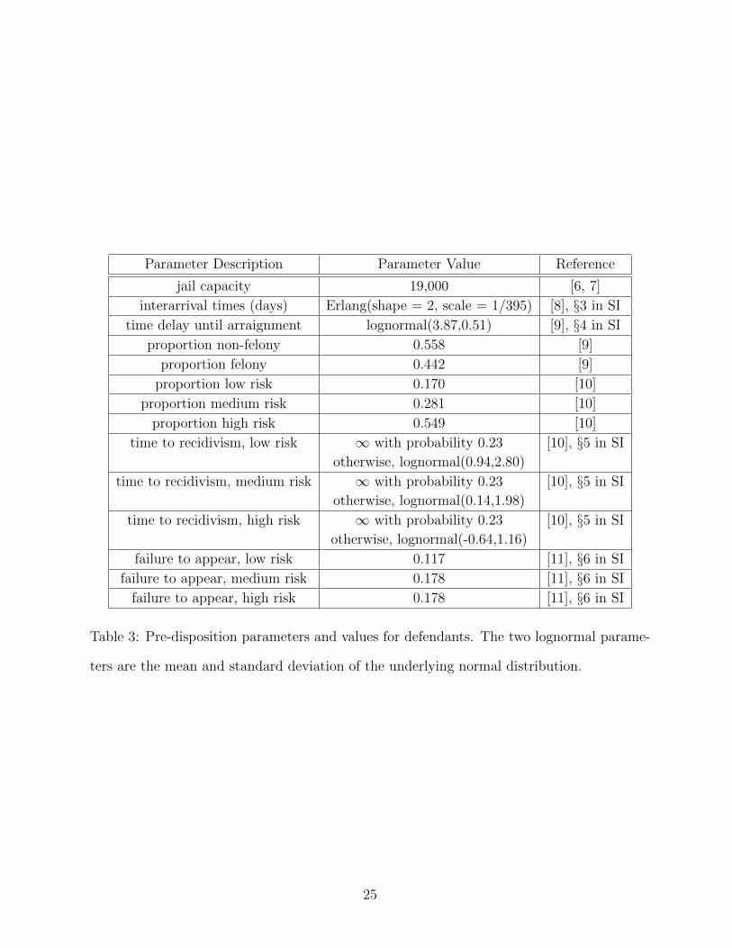
Parameter Description Parameter Value Reference
jail capacity 19,000 [6, 7]
interarrival times (days) Erlang(shape = 2, scale = 1/395) [8], §3 in SI
time delay until arraignment lognormal(3.87,0.51) [9], §4 in SI
proportion non-felony 0.558 [9]
proportion felony 0.442 [9]
proportion low risk 0.170 [10]
proportion medium risk 0.281 [10]
proportion high risk 0.549 [10]
time to recidivism, low risk ∞ with probability 0.23 [10], §5 in SI
otherwise, lognormal(0.94,2.80)
time to recidivism, medium risk ∞ with probability 0.23 [10], §5 in SI
otherwise, lognormal(0.14,1.98)
time to recidivism, high risk ∞ with probability 0.23 [10], §5 in SI
otherwise, lognormal(-0.64,1.16)
failure to appear, low risk 0.117 [11], §6 in SI
failure to appear, medium risk 0.178 [11], §6 in SI
failure to appear, high risk 0.178 [11], §6 in SI
Table 3: Pre-disposition parameters and values for defendants. The two lognormal parame-
ters are the mean and standard deviation of the underlying normal distribution.
25
Page 26
Parameter DescriptionNon-felony Felony
ReferencePretrial Pretrial Pretrial Pretrial
Release Custody Release Custody
time from arraignment gamma gamma lognormal gamma [9], §7 in SI
to disposition (days) (1.07,119.78) (0.46,16.80) (5.13,0.47) (0.67,76.81)
proportion dismissed 0.207 0.052 0.153 0.069 [9], §8 in SI
proportion probation 0.481 0.280 0.681 0.534 [9, 12, 13]
§8 in SI
proportion jail (and 0.312 0.668 0.066 0.208 [9, 12, 13]
(probation if non-felony) §8 in SI
proportion prison — — 0.100 0.189 [9, 12, 13]
§8 in SI
post-sentence jail term gamma gamma lognormal lognormal [9, 14]
(days for non-felony, (0.368,29.92) (0.397,77.08) (1.203,0.633) (2.064,0.628) §9 in SI
months for felony)
length of probation triangular triangular triangular triangular [15, 16]
(years) (0,3,1) (0,3,1) (1,5,3) (1,5,3)
Table 4: Parameters and values related to case disposition. The gamma parameters are the
shape and the scale. The lognormal parameters are the mean and standard deviation of the
underlying normal distribution. The triangular parameters are the minimum, the maximum,
and the mode.
26
Page 27
Statistic Simulation of Reported Values
Status Quo Policy
mean jail population 17,744 ±48 18,693 in 2013 [26]
17,712 in Oct. 2012 [27]
16,448 in Feb. 2012 [6]
felons in jail 14,026 ±43 (79%) 17,259 (0.923) in 2013 [26]
0.78 in Dec. 2011 [6]
non-felons in jail 3718 ±13 (21%) 1434 (0.077) in 2013 [26]
0.22 in Dec. 2011 [6]
sentenced inmates 10,182 ±35 (57.4%) 8845 (0.473) in 2013 [26]
8378 (0.451) in June 2013 [28]
0.55 in Dec. 2011 [6]
non-sentenced inmates 7562 ±19 (42.6%) 9848 (0.527) in 2013 [26]
10,198 (0.549) in June 2013 [28]
0.45 in Dec. 2011 [6]
fraction of time overcrowded 0.151 ±0.009 0.132 in 2012 [8, 26]
Table 5: Model validation of the status quo policy.
Decision Mean Increase in Mean Reduction Risk
Recidivism Exposure (Days) in Jail-Days Ratio
pretrial release of non-felony 128 8 16.0
pretrial release of felony 191 53 3.6
Table 6: The tradeoff and its ratio. The means in the second and third columns are derived
from the gamma and lognormal parameters in Table 4. The risk ratio is the second column
divided by the third column. The risk ratio equals 1.0 for split sentencing of felons.
27
Page 28
Figure Legends
Fig. 1: A depiction of the process flow. The two key decisions (dotted lines) are whether
to offer pretrial release (denoted by PTR?) and split sentencing (SS?), where the latter is
available only to felons. The key tradeoff is between public safety, as measured by recidivism
(dashed lines), and jail population, which is the total number of inmates waiting for arraign-
ment, in pretrial custody or serving a post-sentence jail term. Each arrival has a charge type
(non-felony or felony) and a CSRA risk category (low, medium or high), and some of the
routing probabilities and time durations are functions of charge type, risk category and/or
pretrial status (release or custody).
Fig. 2: For each of the four options for split sentencing in the right column of Table 1, the
optimal (i.e., optimizing over the remaining 16 options in Table 1) tradeoff curves of the
annual rearrest rate vs. (a) the mean jail population and (b) mean jail overcrowding. The
circle denotes the status quo policy for LA County in early 2014.
Fig. 3: For each of the four tradeoff curves in Fig. 2a, the optimal policy along the different
points on the curve. Each policy is denoted by a pair of numbers, where the first number
corresponds to the pretrial release for non-felonies (left column of Table 1) and the second
number corresponds to the pretrial release for felonies (middle column of Table 1).
28
Page 32
SUPPORTING INFORMATION
1 Status Quo Pretrial Release Probabilities
To derive the six probabilities of pretrial release conditioned on risk category and charge
that appear in Table 2 in the main text, we proceed in three steps: compute the pretrial
detention probability conditioned only on risk category, then compute the pretrial detention
probability conditioned only on charge, and then derive the probability of pretrial detention
conditioned jointly on risk and charge.
We first derive the probability that a defendant of each risk category (regardless of
charge) is released prior to trial, using a nationwide study of federal courts [1] and a study
of Salt Lake County (UT) jails [2]. We note that – like LA County – the federal courts and
Salt Lake County allow for commercial bail, bounty hunters and a uniform bail schedule.
On page 31 of [1], risk categories 1 and 2 correspond to low risk, category 3 corresponds
to medium risk, and categories 4 and 5 correspond to high risk. The five risk categories
have equal numbers of defendants in them. By Fig. 23 in [1], the release probabilities are
(0.871+0.623)/2=0.747 for low risk, 0.494 for high risk, and (0.400+0.279)/2=0.3395 for
high risk.
The seven risk categories in [2] are equally probable by construction, with risk cate-
gories 1, 2-3, and 4-7 corresponding to low, medium and high risk (Table 17 in [2]). We denote
the events that a defendant belongs to the low, medium and high risk category by L, M and
H, and denote the events of pretrial release and detention by R and D. Our goal is to compute
conditional probabilities P (R|L), P (R|M) and P (R|H). By construction of the risk categories,
we know P(L)=0.143, P(M)=0.286 and P(H)=0.571. Table 19 of [2] gives the conditional
probabilities P (L|R)=0.43, P (L|D)=0.25, P (M|R)=0.26, P (M|D)=0.22, P (H|R)=0.31 and
P (H|D)=0.53. On page 5 of [2], the sample size includes 4986 defendants with pretrial release
interviews and 2981 without pretrial release interviews. Of a random sample of 1456 from
1
Page 33
the 4986 defendants with pretrial release interviews, 390 were not released. Assuming that
all 2981 defendants without pretrial release interviews were detained, we estimate that (1-
390/1456)4986= 3650 were released and (390/1456)4986+2981 = 4317 were detained, giving
P (R)=0.458 and P (D)=0.542. We substitute all of these probabilities into the law of total
probability to get
P (R|L) =P (L|R)P (R)
P (L|R)P (R) + P (L|D)P (D)= 0.593. (1)
Replacing L in (1) by M and H yields P (R|M)=0.500 and P (R|H)=0.331. Finally, taking
an average of these conditional probabilities over the two studies [1, 2], we assume that the
probability of release for a defendant of low, medium or high risk is 0.667, 0.500 and 0.333,
respectively. Therefore, the conditional probabilities of pretrial detention given risk category
are P (D|L)=0.333, P (D|M)=0.500 and P (D|H)=0.667.
Having derived the pretrial detention probabilities conditioned on risk, we now compute
the pretrial detention probabilities conditioned on charge. By the top right box on page 79
of [3], the probability that a felon in LA County was released is 0.23 and the probability that
a defendant with a non-felony in LA County was released is 0.66. Letting N denote non-
felony and F denote felony, the conditional probabilities of pretrial detention given charge are
P (D|N)=0.34 and P (D|F)=0.77. Using the risk proportions in Table 1 of the main text, we
find that the probability of being detained is P (D)=0.549(0.667)+0.281(0.500)+0.170(0.333)
=0.563.
Our goal now is to derive a mathematical expression for the conditional probability
of pretrial detention given the charge type C (either N or F) and risk category R (either
L, M or H), which we denote by P (D|C,R), in terms of the probabilities P (D|R), P (D|C)
and P (D) calculated above. By our assumption that C and R are independent, it follows
that P (C|R)=P (C) and P (C|R,D)=P (C|D). By the definition of conditional probability, we
have P (C|D)=P (C,D)/P (D) and P (C|R,D)=P (C,D|R)/P (D|R). Substituting the right sides
2
Page 34
of these two equations into P (C|R,D)=P (C|D) yields P (C,D|R)/P (D|R)=P (C,D)/P (D).
Substituting P (D|C)P (C) for P (C,D) in this equation and rearranging gives
P (C,D|R)
P (C)=P (D|C)P (D|R)
P (D). (2)
Finally, we find that
P (D|C,R) =P (D,C|R)
P (C|R), (3)
=P (D,C|R)
P (C)because C and R are independent, (4)
=P (D|C)P (D|R)
P (D)by (2). (5)
Substituting the numerical values above into the right side of (5) and then noting that the
conditional probability of release given crime type and risk category is 1-P (D|C,R), we get
the conditional release probabilities in Table 2 of the main text.
2 Pretrial Release After Recidivism
According to Table 2 of [3], 20-21% of felons in LA County receive financial release. Table 19
in the Appendix of [4] states that 19% of felons receive financial release in LA County,
confirming the numbers in [3]. When averaged over the 75 largest counties in the U.S.,
Table 6 in [4] states that 33% of felons receive financial release and Table 8 in [4] states that
18% of felons with custody history receive financial release. Extrapolating these nationwide
numbers back to LA County, we estimate that 18(19)/33=10.4% of felons in LA County
with custody history receive financial release. For lack of data on non-felony defendants, we
assume that 20% (10%, respectively) of defendants charged with non-felonies (respectively,
felonies) during a recidivism event receive financial release.
3
Page 35
3 Interarrival Times
The arraignments under custody from the LA County Sheriff’s Department’s Year in Review
reports (e.g., [5]) for the years 2008-2012 give an average of 350.4/day with no obvious long-
term trend (Table 1). There is little variability over the time of year (page 36 of Appendix C
in [3]), and we ignore the fact that fewer arraignments occur over the weekend (page 34
of Appendix C in [3]). We estimate the squared coefficient of variation (i.e., the variance
divided by the square of the mean) of the interarrival times to be 0.465 from the data
in Table 1 by assuming that the times between consecutive arrivals are independent and
identically distributed. The Erlang distribution is characterized by its shape parameter and
scale parameter. The Erlang shape parameter is the reciprocal of the squared coefficient
of variation, and so we set the shape parameter equal to two. The mean of an Erlang
distribution is the product of its shape and scale parameters. Because the arrival rate of
350/day includes recidivists, who account for slightly less than half of the total number of
arrivals, we adjust the rate of new arrivals to be 193/day so that the total arrival rate is
350/day. This yields a shape parameter of 1/395.
4 Time to Arraignment
Arraignment data from LA County in 2008 states that 4% of defendants were arraigned
within 24 hours of arrest, 56.4% were arraigned within 48 hours, 70.4% were arraigned
within 72 hours, and 95% were arraigned within 96 hours (page 63 of [3]). The maximum
likelihood estimate for the lognormal parameters from these data yield the values in Table 3
of the main text.
4
Page 36
5 Time to Recidivism
Let the cumulative distribution function (CDF) F (t; Θ, j) be the probability that an offender
recidivates within t time units of being released, given that he is of risk category j (where
j = 1, 2, 3 correspond to low, medium and high risk) under parameter set Θ. These CDFs
are specified for our five models in Table 2. Let Nj be the number of offenders in the CSRA
cohort [6] with risk category j, where N =∑3
j=1 Nj. Let Njk be the number of offenders
in the CSRA cohort with risk category j that did not recidivate within k − 1 years but did
recidivate within k years. The data from [6] are N = 110, 313, N1 = 18, 768, N2 = 31, 024,
N3 = 60, 521, N11 = 4845, N12 = 1681, N13 = 641, N21 = 12, 002, N22 = 3403, N23 = 1269,
N31 = 33, 243, N32 = 7925 and N33 = 2584. We choose the values of Θ to maximize the
log-likelihood function,
3∑j=1
Nj1 logF (1; Θ, j) +3∑j=1
Nj2 log(F (2; Θ, j)− F (1; Θ, j))
+3∑j=1
Nj3 log(F (3; Θ, j)− F (2; Θ, j)) +3∑j=1
(Nj −Nj1 −Nj2 −Nj3) log(1− F (3; Θ, j)). (6)
The estimation results (Table 3) suggest that the lognormal models outperform the
proportional hazards models (as measured by the negative log-likelihood values), and the
split is statistically significant in the lognormal model only if we incorporate risk-associated
heteroskedasticity. We use the split lognormal model with heteroskedasticity, and the three
probability density functions (one for each risk category) are pictured in Fig. 1. Using
quarterly average cumulative recidivism probabilities for three years from Fig. 2 of [6], we
perform a granular cross-validation and find that the pointwise root mean square error
between the predicted (by the split lognormal model with heteroskedaticity) and actual
probabilities is 0.022, with a pointwise maximum difference of 0.049.
5
Page 37
6 Failure To Appear
We use a validation study of COMPAS for predicting failure to appear in court in Broward
County, FL [7]. COMPAS’s 10 risk scores were aggregated into CSRA’s three risk categories,
where scores 1-4, 5-7 and 8-10 correspond to low, medium and high risk (page 20 of [7]).
Table 13 in [7] gives failure-to-appear probabilities for the three risk groups at six different
follow-up periods, but does not provide information on the time from arraignment to dis-
position. Hence, we cannot attempt to estimate (e.g., via logistic regression) whether the
failure-to-appear probability depends on the arraignment-to-disposition delay. To minimize
right-censoring (i.e., due to a case disposition date that is far in the future), we use their
largest follow-up period of 12 months; these data are reproduced in Table 4. Because the
failure-to-appear probability is slightly higher for medium risk than high risk (the same is
true for follow-up periods of three months and six months in Table 13 in [7]), we combine
medium risk and high risk in our analysis. Hence, we assume that the failure-to-appear
probability is 0.117 for low risk and is [456(0.180)+163(0.172)]/(456+163)=0.178 for both
medium risk and high risk.
7 Time from Arraignment to Case Disposition
Because the time from arrest to arraignment is typically much smaller than the time from
arraignment to disposition, we use arrest-to-disposition time data from pages 55-56 in [3],
which appear in Table 5, to estimate the time from arraignment to disposition, using both
gamma and lognormal distributions. Lognormal provides a better fit (using the Kolmogorov
distances in Table 5) for felonies in pretrial release, and gamma (with an increasing failure
rate for those released and a decreasing failure rate for those in custody) provides a better
fit for felonies under pretrial custody and for all non-felonies.
6
Page 38
8 Case Disposition Probabilities
The 14 case disposition probabilities in Table 4 in the main text are derived in three groups.
Ignoring the ongoing cases in Table 4 of [3] and combining acquitted and dismissed cases,
we estimate the four proportion dismissed values that appear in Table 4 in the main text
(e.g., for felons on pretrial release, (1635+46)/(12,154-1168)=0.153).
We denote the proportion of non-felony charges that are put on probation after pretrial
release, put on probation after pretrial custody, receive a jail sentence after pretrial release
and receive a jail sentence after pretrial custody by p1, p2, p3 and p4, respectively. We
jointly solve for these four unknowns using four equations. The first two equations use the
proportion dismissed values, 0.207 and 0.052, in Table 4 in the main text:
p1 + p3 = 1− 0.207, (7)
p2 + p4 = 1− 0.052. (8)
The third equation specifies that the proportion of all non-felony charges that result in jail
sentences is 7310/16,891 = 0.433 (page 129 of [3]):
0.66p3 + (1− 0.66)p4 = 0.433, (9)
where 0.66 was estimated in §1. The final equation uses the result that the odds ratio to be
jailed for a non-felony in pretrial custody relative to a non-felony under pretrial release is
4.44 (page 10 in [8]):
p4(1− p3)
p3(1− p4)= 4.44. (10)
Solving (7)-(10) jointly gives the proportions in Table 4 in the main text.
The remaining six case disposition probabilities are derived jointly. We denote the
proportion of felons who are put on probation after pretrial release, put on probation after
pretrial custody, receive a jail sentence after pretrial release, receive a jail sentence after
7
Page 39
pretrial custody, are sent to prison after pretrial release, and are sent to prison after pretrial
custody by p5, p6, p7, p8, p9 and p10, respectively. We jointly solve for these six unknowns
using six equations. The first two equations use the proportion dismissed values, 0.153 and
0.069:
p5 + p7 + p9 = 1− 0.153, (11)
p6 + p8 + p10 = 1− 0.069. (12)
The third equation states that the proportion of felons that get probation is, using the last
four columns in Table 1 in [9], 23,476/41,725=0.563:
0.23p5 + (1− 0.23)p6 = 0.563, (13)
where 0.23 was estimated in §1. Similarly, the fourth equation specifies that the proportion
of all felons that receive jail sentences is (7407+125)/41,725 = 0.181 (the last four columns
in Table 1 in [9]):
0.23p7 + (1− 0.23)p8 = 0.181. (14)
As in (10), the fifth equation uses the result that the odds ratio to be jailed for a felony in
pretrial custody relative to a felony under pretrial release is 3.32 (page 10 in [8]):
(p8 + p10)(1− p7 − p9)
(p7 + p9)(1− p8 − p10)= 3.32. (15)
The sixth equation states that the probability of pretrial release given a prison charge (as
opposed to a prison sentence) is 0.15 (page 57 in [3]), which we derive using Bayes rule as
follows. Using the proportion dismissed values 0.153 and 0.069, we find that the probability
of a prison charge given pretrial release is p9/(1 − 0.153), and the probability of a prison
charge given pretrial custody is p10(1−0.069). Because the probability of pretrial release for
8
Page 40
a felony is 0.23 (§1), it follows from Bayes rule that the sixth equation is
0.23(
p91−0.153
)0.23
(p9
1−0.153
)+ (1− 0.23)
(p10
1−0.069
) = 0.15. (16)
Simultaneously solving (11)-(16) gives the proportions in Table 4 in the main text.
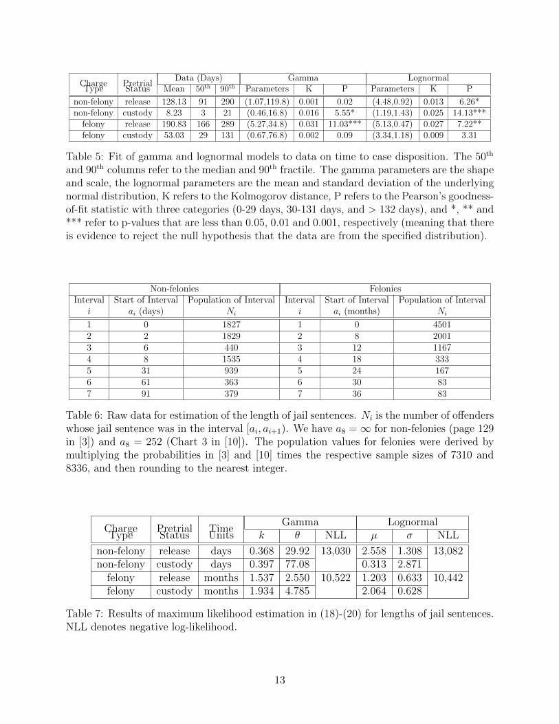
9 Post-sentence Jail Terms
We fit mixture (of pretrial release and pretrial custody) gamma and lognormal distributions
for jail sentences for non-felonies using data on page 129 in [3] and Fig. 25 in Appendix C in
[3], and for jail sentences for felonies using data in Chart 3 in [10]. The data (reproduced in
Table 6) are of the form: Ni offenders have jail terms in the interval (ai, ai+1] for i = 1, . . . , 7,
where∑7
i=1Ni = N . We consider the mixture CDF
F (x; Θ) =wR
wR + wDG(x; ΘR) +
wDwR + wD
G(x; ΘD), (17)
where R and D denote the populations that are in pretrial release and pretrial detention,
respectively, and wR and wD are weights proportional to the sizes of these two populations.
Because 66% of non-felonies and 23% of felonies receive pretrial release (§1), and 55.8%
of defendants are charged with felonies (Table 3 of the main text), we have that wR =
0.66(0.558) = 0.368 and wD = 0.34(0.558) = 0.190 for non-felonies, and wR = 0.23(0.442) =
0.102 and wD = 0.77(0.442) = 0.340 for felonies. We consider two cases: G(x) is lognormal
with parameters (µ, σ) and G(x) is gamma with scale parameter k and shape parameter θ,
where R and D are subscripts on the parameters in (17) to denote the released or detained
populations. We use a constrained maximum likelihood approach, where we require the
mean jail sentence for non-felonies to be 2.78 times longer for those undergoing pretrial
detention relative to those receiving pretrial release, and the mean jail sentence for felonies
to be 2.36 times longer for those undergoing pretrial detention relative to those receiving
9
Page 41
pretrial release (page 10 of [8]). Hence, setting r = 2.78 for non-felonies and r = 2.36 for
felonies, and setting F (0; Θ) = 0 and F (∞; Θ) = 1, we solve
minΘ=(ΘR,ΘD)
−7∑i=1
Ni ln(F (ai+1; Θ)− F (ai; Θ)), (18)
subject to eµD+σ2D/2 = reµR+σ2
R/2 if G(x) is lognormal, (19)
subject to kDθD = rkRθR if G(x) is gamma. (20)
The results appear in Table 7, and we adopt the distribution with the lower negative log-
likelihood: gamma for non-felonies and lognormal for felonies.
10
Page 42
References
[1] VanNostrand, M., Keebler, G. Pretrial risk assessment in the federal court. U.S. Dept.
of Justice, Washington, D.C., April 14, 2009.
[2] Hickert, A., Worwood, E. B., Prince, K. Pretrial release risk study, validation, & scoring:
final report. Utah Criminal Justice Center, U. of Utah, Salt Lake City, UT, April 2013.
[3] Vera Institute of Justice. Los Angeles County jail overcrowding reduction project, final
report: revised. Vera Institute of Justice, New York, September 2011.
[4] Bureau of Justice Statistics. Felony defendants in large urban counties, 2006. Bureau of
Justice Statistics Bulletin, NCJ 228944, May 2010.
[5] LA County Sheriff’s Department. Year in review 2012. Monterey Park, CA, 2013.
[6] Beard, J., Toche, D., Beyer, B., Babby, W., Allen, D., Grassel, K., Maxwell, D., Nakao,
M. 2013 outcome evaluation report. California Department of Corrections and Rehabil-
itation, January 2014.
[7] Blomberg, T., Bales, W., Mann, K., Meldrum, R., Nedelec, J. Validation of the COM-
PAS risk assessment classification instrument. College of Criminology and Criminal
Justice, Florida State University, Tallahassee, FL, September 2010.
[8] Lowenkamp, C. T., VanNostrand, M., Holsinger, A. Investigating the impact of pretrial
detention on sentencing outcomes. Laura and John Arnold Foundation report, Houston,
TX, November 2013.
[9] Jahr, S. Court realignment data - calendar year 2013. Judicial Council of CA, San
Francisco, CA, August 22, 2014.
[10] Delgado, M. Public safety realignment implementation update - year one report. Coun-
tywide Criminal Justice Coordination Committee, November 28, 2012.
11
Page 43
Year Number of Arraignments Under Custody
2008 122,4362009 126,3522010 130,9592011 134,2712012 125,965
Table 1: Raw data to estimate the interarrival time distribution [5].
Model Parameter Set CDF(Sign Constraint)
lognormal β(−), µ, σ(+) 12
(1 + erf
(ln t−µ−βT x√
2σ
))split lognormal β(−), µ,σ(+), δ(+) δ
2
(1 + erf
(ln t−µ−βT x√
2σ
))split lognormal with heteroskedasticity β(−), µ,σ(+), δ(+), γ(−) δ
2
(1 + erf
(ln t−µ−βT x√
2(σ+γT x)
))proportional hazards β(+), λ 1− e(−λt)eβx
split proportional hazards β(+), λ, δ(+) δ(
1− e(−λt)eβx)
Table 2: Five survival models for time to recidivism.
Model β µ σ δ γ λ NLL p-value
lognormal -1.10 2.94 2.59 118,698 base-(1.13,1.07) (2.87,3.01) (2.55,2.63)
split lognormal -1.10 2.94 2.59 1.00 118,698 1.00split lognormal -0.80 1.74 3.62 0.77 -0.82 118,310 < 10−3
heteroskedasticity -(0.84,0.76) (1.64,1.84) (3.51,3.74) (0.76,0.78) -(0.78,0.87)proportional 0.56 0.10 129,390 base
hazardssplit proportional 0.69 0.69 0.18 120,522 < 10−3
hazards
Table 3: Results from the maximum likelihood estimation in (6), with 95% confidence in-tervals in parentheses for the two models that provide the best fit. NLL is negative log-likelihood, and p-value is the likelihood ratio test of the enhanced model relative to the base(lognormal or proportional hazards) model.
Risk Category Sample Size Failure-to-Appear Probability
low 1901 0.117medium 456 0.180
high 163 0.172
Table 4: Raw data for estimation of the failure-to-appear probabilities, reproduced fromTable 13 in [7]. The sample size is the number of defendants in each risk category whodid not recidivate during their first 12 months under pretrial release. The failure-to-appearprobability is the proportion of these defendants who failed to appear for a court date duringtheir first 12 months of pretrial release.
12
Page 44
Charge PretrialData (Days) Gamma Lognormal
Type Status Mean 50th 90th Parameters K P Parameters K P
non-felony release 128.13 91 290 (1.07,119.8) 0.001 0.02 (4.48,0.92) 0.013 6.26*non-felony custody 8.23 3 21 (0.46,16.8) 0.016 5.55* (1.19,1.43) 0.025 14.13***
felony release 190.83 166 289 (5.27,34.8) 0.031 11.03*** (5.13,0.47) 0.027 7.22**felony custody 53.03 29 131 (0.67,76.8) 0.002 0.09 (3.34,1.18) 0.009 3.31
Table 5: Fit of gamma and lognormal models to data on time to case disposition. The 50th
and 90th columns refer to the median and 90th fractile. The gamma parameters are the shapeand scale, the lognormal parameters are the mean and standard deviation of the underlyingnormal distribution, K refers to the Kolmogorov distance, P refers to the Pearson’s goodness-of-fit statistic with three categories (0-29 days, 30-131 days, and > 132 days), and *, ** and*** refer to p-values that are less than 0.05, 0.01 and 0.001, respectively (meaning that thereis evidence to reject the null hypothesis that the data are from the specified distribution).
Non-felonies FeloniesInterval Start of Interval Population of Interval Interval Start of Interval Population of Interval
i ai (days) Ni i ai (months) Ni
1 0 1827 1 0 45012 2 1829 2 8 20013 6 440 3 12 11674 8 1535 4 18 3335 31 939 5 24 1676 61 363 6 30 837 91 379 7 36 83
Table 6: Raw data for estimation of the length of jail sentences. Ni is the number of offenderswhose jail sentence was in the interval [ai, ai+1). We have a8 =∞ for non-felonies (page 129in [3]) and a8 = 252 (Chart 3 in [10]). The population values for felonies were derived bymultiplying the probabilities in [3] and [10] times the respective sample sizes of 7310 and8336, and then rounding to the nearest integer.
Charge Pretrial TimeGamma Lognormal
Type Status Units k θ NLL µ σ NLL
non-felony release days 0.368 29.92 13,030 2.558 1.308 13,082non-felony custody days 0.397 77.08 0.313 2.871
felony release months 1.537 2.550 10,522 1.203 0.633 10,442felony custody months 1.934 4.785 2.064 0.628
Table 7: Results of maximum likelihood estimation in (18)-(20) for lengths of jail sentences.NLL denotes negative log-likelihood.
13
Page 45
Fig. 1: The lognormal probability density functions for the time to recidivism for the threerisk categories.
14
Page 46
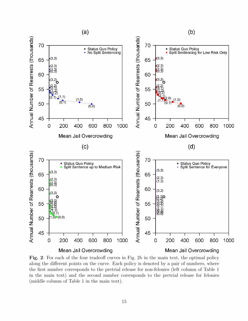
Fig. 2: For each of the four tradeoff curves in Fig. 2b in the main text, the optimal policyalong the different points on the curve. Each policy is denoted by a pair of numbers, wherethe first number corresponds to the pretrial release for non-felonies (left column of Table 1in the main text) and the second number corresponds to the pretrial release for felonies(middle column of Table 1 in the main text).
15
Page 47
Fig. 3: For each of the four options for split sentencing in the right column of Table 1, theoptimal (i.e., optimizing over the remaining 16 options in Table 1) tradeoff curves of theannual rearrest rate vs. (a) the mean jail population and (b) mean jail overcrowding,restricting to policies that treat felonies at least as strictly (with respect to pretrial release)as non-felonies of the same risk category. The circle denotes the status quo policy for LACounty in early 2014.
16