Page 1
Assessing the applicability of the ASME V&V20 Standard forUncertainty Quantification of CFD in Nuclear Systems Fluid Modeling
by
Andres Felipe Alvarez
Submitted to the Department of Nuclear Science and Engineeringin partial fulfillment of the requirements for the degree of
Bachelor of Science in Nuclear Science and Engineering
at the
Massachusetts Institute of Technology
June 2017
c©2017 Massachusetts Institute of Technology. All rights reserved.
Author . . . . . . . . . . . . . . . . . . . . . . . . . . . . . . . . . . . . . . . . . . . . . . . . . . . . . . . . . . . . . . . . . . . . . . . . . . . .Department of Nuclear Science and Engineering
May 18, 2017
Certified by. . . . . . . . . . . . . . . . . . . . . . . . . . . . . . . . . . . . . . . . . . . . . . . . . . . . . . . . . . . . . . . . . . . . . . . .Emilio Baglietto
Norman C. Rasmussen Associate Professor, Nuclear Science and EngineeringThesis Supervisor
Accepted by . . . . . . . . . . . . . . . . . . . . . . . . . . . . . . . . . . . . . . . . . . . . . . . . . . . . . . . . . . . . . . . . . . . . . . .Michael Short
Assistant Professor, Nuclear Science and EngineeringChair, NSE Department Committee for Undergraduate Students
Page 3
Assessing the applicability of the ASME V&V20 Standard
for Uncertainty Quantification of CFD in Nuclear Systems
Fluid Modeling
by
Andres Felipe Alvarez
Submitted to the Department of Nuclear Science and Engineeringon May 18, 2017, in partial fulfillment of the
requirements for the degree ofBachelor of Science in Nuclear Science and Engineering
Abstract
Advanced modeling and simulation (M&S) of nuclear systems could offer a key con-tribution in enhancing the competitiveness and safety performance of nuclear powerplants. Large multi-organizational initiatives such as the Consortium for AdvancedSimulation of Light Water Reactors (CASL) and the Nuclear Energy Advanced Mod-eling and Simulation (NEAMS) emphasizes the importance of M&S research to theU.S. nuclear industry. Uncertainty Quantification (UQ) represents a fundamentalarea of research necessary to expand the application of M&S into nuclear industry,but the field is still not mature, and no general consensus exists on current UQ meth-ods. In this study, the ASME V&V20 — a proposed methodology for UQ of CFD —is applied to a benchmark nuclear system turbulent mixing case in an effort to assessthe applicability and limitations of the standard.
Thesis Supervisor: Emilio BagliettoTitle: Norman C. Rasmussen Associate Professor, Nuclear Science and Engineering
3
Page 5
Acknowledgments
I would like to first, and foremost thank Professor Emilio Baglietto for his time and
guidance in the development of this report. Professor Baglietto has served as an
incredible mentor for me, showing great patience and encouragement during my time
at MIT. It was a true honor to serve as one of his first undergraduate students at
MIT.
Secondly, I would also like to thank all those who contributed to the research
in this study. Thank you to Etienne Demarly, Ravi Kishore, and Ben Magolan for
helping get started in my research during the summer of 2016. A special thanks to
Mike Acton for taking the time to review UQ methodology with me and for helping
in the revision of this thesis. Finally, thank you Professor Short for taking the time
to review this thesis and ensure its quality.
Professor Neil Todreas has served as role model for me during my four years of
undergraduate studies at MIT. I cannot express how much I have appreciated his
mentorship, friendship, encouragement and wisdom. I want to thank him for taking
me under his supervision and for teaching me the fundamentals of great engineering
leadership.
During my time working on this study, I was blessed to be surrounded by friendly
and caring peers. I would like to thank the Nuclear Department’s class of 2017 for
their friendship and support. I would also like to give a thank you to Heather Barry
for helping create a welcoming community in the Nuclear Department. A thank
you to my fellow brothers at Phi Kappa Sigma who I have shared countless great
experiences with. I would like to recognize the MIT Gordon Engineering Leadership
Program and its participants for instilling in me fundamental leadership principles.
Lastly, I would like to thank the MIT Energy club for letting me serve as their Vice
President and for the incredible opportunities associated with the role.
Finally, I would like to thank my parents for supporting me throughout my entire
life. They sacrificed a lot to make it to the United States. This degree will ensure
that their efforts were not to waste.
5
Page 7
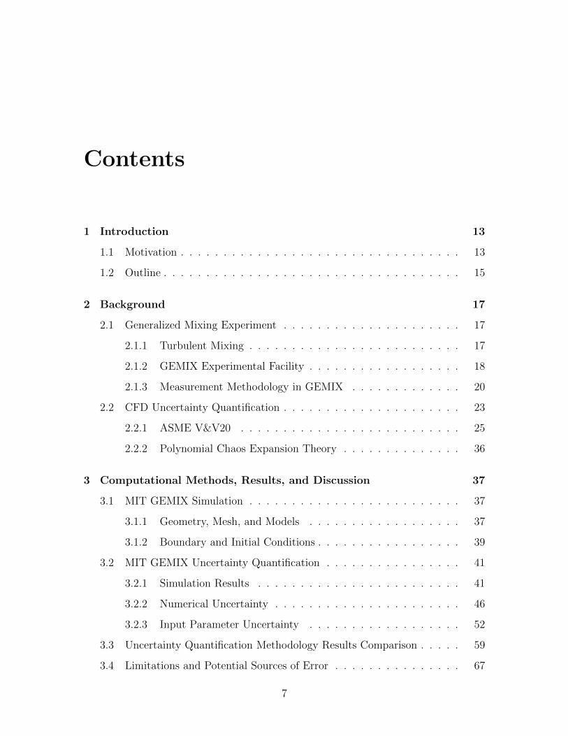
Contents
1 Introduction 13
1.1 Motivation . . . . . . . . . . . . . . . . . . . . . . . . . . . . . . . . . 13
1.2 Outline . . . . . . . . . . . . . . . . . . . . . . . . . . . . . . . . . . . 15
2 Background 17
2.1 Generalized Mixing Experiment . . . . . . . . . . . . . . . . . . . . . 17
2.1.1 Turbulent Mixing . . . . . . . . . . . . . . . . . . . . . . . . . 17
2.1.2 GEMIX Experimental Facility . . . . . . . . . . . . . . . . . . 18
2.1.3 Measurement Methodology in GEMIX . . . . . . . . . . . . . 20
2.2 CFD Uncertainty Quantification . . . . . . . . . . . . . . . . . . . . . 23
2.2.1 ASME V&V20 . . . . . . . . . . . . . . . . . . . . . . . . . . 25
2.2.2 Polynomial Chaos Expansion Theory . . . . . . . . . . . . . . 36
3 Computational Methods, Results, and Discussion 37
3.1 MIT GEMIX Simulation . . . . . . . . . . . . . . . . . . . . . . . . . 37
3.1.1 Geometry, Mesh, and Models . . . . . . . . . . . . . . . . . . 37
3.1.2 Boundary and Initial Conditions . . . . . . . . . . . . . . . . . 39
3.2 MIT GEMIX Uncertainty Quantification . . . . . . . . . . . . . . . . 41
3.2.1 Simulation Results . . . . . . . . . . . . . . . . . . . . . . . . 41
3.2.2 Numerical Uncertainty . . . . . . . . . . . . . . . . . . . . . . 46
3.2.3 Input Parameter Uncertainty . . . . . . . . . . . . . . . . . . 52
3.3 Uncertainty Quantification Methodology Results Comparison . . . . . 59
3.4 Limitations and Potential Sources of Error . . . . . . . . . . . . . . . 67
7
Page 8
4 Conclusion & Future Work 69
Bibliography 72
8
Page 9
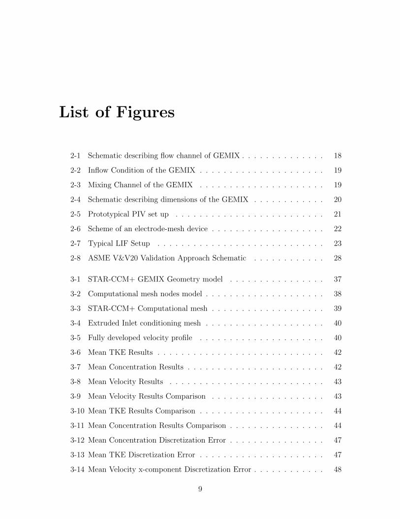
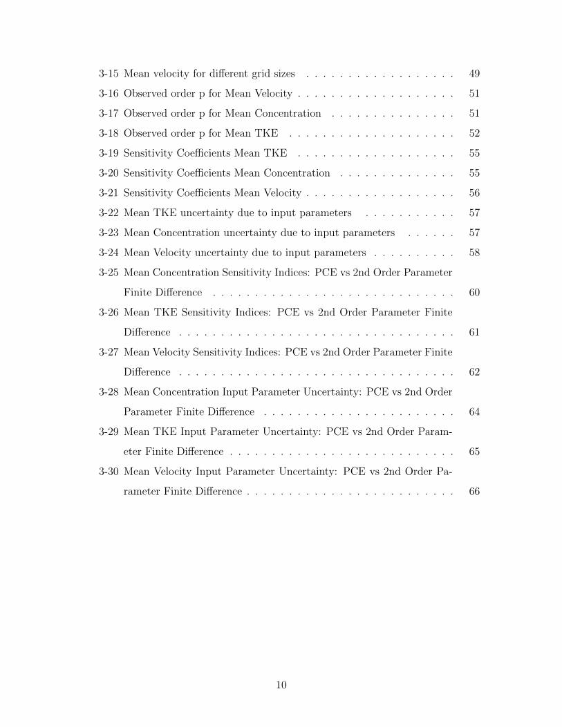
List of Figures
2-1 Schematic describing flow channel of GEMIX . . . . . . . . . . . . . . 18
2-2 Inflow Condition of the GEMIX . . . . . . . . . . . . . . . . . . . . . 19
2-3 Mixing Channel of the GEMIX . . . . . . . . . . . . . . . . . . . . . 19
2-4 Schematic describing dimensions of the GEMIX . . . . . . . . . . . . 20
2-5 Prototypical PIV set up . . . . . . . . . . . . . . . . . . . . . . . . . 21
2-6 Scheme of an electrode-mesh device . . . . . . . . . . . . . . . . . . . 22
2-7 Typical LIF Setup . . . . . . . . . . . . . . . . . . . . . . . . . . . . 23
2-8 ASME V&V20 Validation Approach Schematic . . . . . . . . . . . . 28
3-1 STAR-CCM+ GEMIX Geometry model . . . . . . . . . . . . . . . . 37
3-2 Computational mesh nodes model . . . . . . . . . . . . . . . . . . . . 38
3-3 STAR-CCM+ Computational mesh . . . . . . . . . . . . . . . . . . . 39
3-4 Extruded Inlet conditioning mesh . . . . . . . . . . . . . . . . . . . . 40
3-5 Fully developed velocity profile . . . . . . . . . . . . . . . . . . . . . 40
3-6 Mean TKE Results . . . . . . . . . . . . . . . . . . . . . . . . . . . . 42
3-7 Mean Concentration Results . . . . . . . . . . . . . . . . . . . . . . . 42
3-8 Mean Velocity Results . . . . . . . . . . . . . . . . . . . . . . . . . . 43
3-9 Mean Velocity Results Comparison . . . . . . . . . . . . . . . . . . . 43
3-10 Mean TKE Results Comparison . . . . . . . . . . . . . . . . . . . . . 44
3-11 Mean Concentration Results Comparison . . . . . . . . . . . . . . . . 44
3-12 Mean Concentration Discretization Error . . . . . . . . . . . . . . . . 47
3-13 Mean TKE Discretization Error . . . . . . . . . . . . . . . . . . . . . 47
3-14 Mean Velocity x-component Discretization Error . . . . . . . . . . . . 48
9
Page 10
3-15 Mean velocity for different grid sizes . . . . . . . . . . . . . . . . . . 49
3-16 Observed order p for Mean Velocity . . . . . . . . . . . . . . . . . . . 51
3-17 Observed order p for Mean Concentration . . . . . . . . . . . . . . . 51
3-18 Observed order p for Mean TKE . . . . . . . . . . . . . . . . . . . . 52
3-19 Sensitivity Coefficients Mean TKE . . . . . . . . . . . . . . . . . . . 55
3-20 Sensitivity Coefficients Mean Concentration . . . . . . . . . . . . . . 55
3-21 Sensitivity Coefficients Mean Velocity . . . . . . . . . . . . . . . . . . 56
3-22 Mean TKE uncertainty due to input parameters . . . . . . . . . . . 57
3-23 Mean Concentration uncertainty due to input parameters . . . . . . 57
3-24 Mean Velocity uncertainty due to input parameters . . . . . . . . . . 58
3-25 Mean Concentration Sensitivity Indices: PCE vs 2nd Order Parameter
Finite Difference . . . . . . . . . . . . . . . . . . . . . . . . . . . . . 60
3-26 Mean TKE Sensitivity Indices: PCE vs 2nd Order Parameter Finite
Difference . . . . . . . . . . . . . . . . . . . . . . . . . . . . . . . . . 61
3-27 Mean Velocity Sensitivity Indices: PCE vs 2nd Order Parameter Finite
Difference . . . . . . . . . . . . . . . . . . . . . . . . . . . . . . . . . 62
3-28 Mean Concentration Input Parameter Uncertainty: PCE vs 2nd Order
Parameter Finite Difference . . . . . . . . . . . . . . . . . . . . . . . 64
3-29 Mean TKE Input Parameter Uncertainty: PCE vs 2nd Order Param-
eter Finite Difference . . . . . . . . . . . . . . . . . . . . . . . . . . . 65
3-30 Mean Velocity Input Parameter Uncertainty: PCE vs 2nd Order Pa-
rameter Finite Difference . . . . . . . . . . . . . . . . . . . . . . . . . 66
10
Page 11
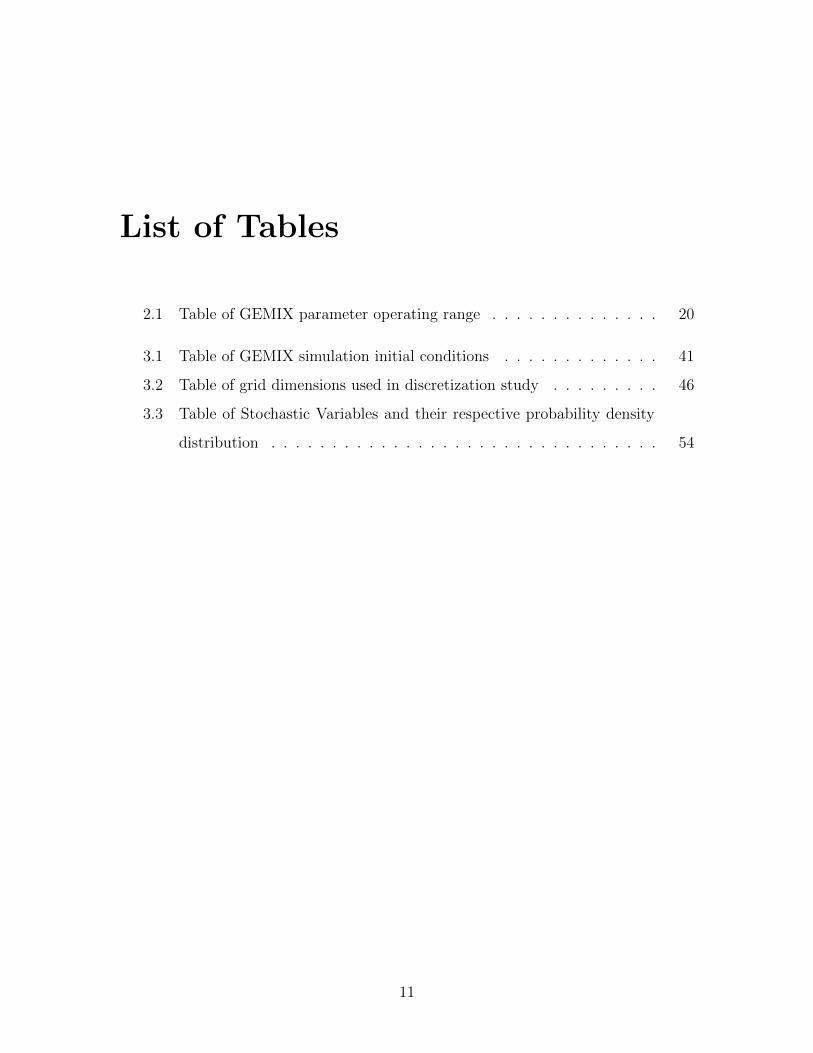
List of Tables
2.1 Table of GEMIX parameter operating range . . . . . . . . . . . . . . 20
3.1 Table of GEMIX simulation initial conditions . . . . . . . . . . . . . 41
3.2 Table of grid dimensions used in discretization study . . . . . . . . . 46
3.3 Table of Stochastic Variables and their respective probability density
distribution . . . . . . . . . . . . . . . . . . . . . . . . . . . . . . . . 54
11
Page 13
Chapter 1
Introduction
1.1 Motivation
In the contemporary U.S. market, nuclear power is playing an important role in
baseload and clean energy production. In 2015, the United States produced 19.5
percent of its electricity from nuclear power. [1] In 2014, nuclear energy provided
62.9 percent of carbon free electricity in the United States. [2] As part of an effort to
maintain and improve the performance and safety of nuclear power plants the United
States has dedicated 82 million dollars in 2016 to nuclear energy research. [3]
A significant portion of this U.S. nuclear energy research effort is in advanced
modeling and simulation (M&S), with two notable U.S. led initiatives being the Nu-
clear Energy Advanced Modeling and Simulation (NEAMS) program and Consortium
for Advanced Simulation of Light Water Reactors (CASL). The U.S. Department of
Energy’s (DOE) NEAMS program aims at developing a simulation tool kit that uses
leading-edge computational methods to accelerate the development and deployment
of nuclear power technologies that employ enhanced safety and security features,
produce power more cost-effectively, and utilize natural resources more efficiently.[4]
Another U.S. DOE M&S initative is the Consortium for Advanced Simulation of
Light Water Reactors (CASL) which aims at providing coupled, high fidelity, us-
able capabilities needed to address light water reactor (LWR) operational and safety
performance-defining phenomena. [5] Collaboration between the two initiatives exists,
13
Page 14
with particular emphasis creating tools that can simulate safety defining phenomena
in nuclear reactors such departure from nucleate boiling (DNB), CRUD accumulation
on fuel assemblies, and grid-to-rod fretting (GTRF).
In certain key areas of nuclear systems modeling, such as DNB modeling, tradi-
tional thermal hydraulic codes are insufficiently accurate and fail to capture smaller
details in the physical phenomenon occurring. DNB is when a rapid heat transfer
decrease occurs as a result of an insulating steam blanket that forms on the fuel rod
surface as temperature increases. [3] In order to avoid fuel damage within a pressur-
ized water reactors (PWR) the DNB ratio limit must not be reached. Hence, greater
accuracy in DNB modeling would enhance safety and performance of PWRs.
Computational fluid dynamics (CFD) has been introduced in nuclear systems
modeling as part of the U.S. effort to develop tools that can accurately model nuclear
safety performance defining phenomenon, such as DNB, GTRF, and CRUD build-on.
Tools like CFD are useful for studying nuclear systems because it allows for more
accurate simulation of localized fluid phenomena that are either not reproducible
experimentally or extremely costly to evaluate. For example, fuel rod failure due to
grid-to-rod fretting (GTRF) – fretting wear caused by flow induced vibrations on
grid supports and the fuel rod – accounted for over 70% of the fuel leaks in U.S.
pressurized water reactors (PWRs). CFD offers greater accuracy in computing the
flow turbulence force that drive these fuel rod vibrations. Thus, analysis of localized
turbulent forces from CFD simulations can provide valuable insight into the cause of
these fuel rod failures which would otherwise be unobtainable experimentally or with
traditional thermal hydraulic codes.
An area of CFD that requires particular attention is validation and verification.
CFD has proven to be a reliable tool when used properly, but in order to extend its
application to nuclear systems and to allow for its more consistent adoption there
exists a need establish a methodology for quantifying uncertainties and errors in the
results. Several methodologies for evaluating error and uncertainty caused by mesh
refinement and input parameters have been proposed in the past, but it has not been
until recently in 2009 that a verification and validation standard was published by the
14
Page 15
American Society of Mechanical Engineers (ASME). [6] Prior to the utilization of this
CFD uncertainty quantification methodology in the nuclear industry an assessment
of the applicability and limitations of this AMSE V&V20 standard is required.
This study focuses on performing uncertainty quantification work for simulations
of the generic mixing experiment (GEMIX) in an effort to better understand the ap-
plicability of the ASME V&V20 standard to CFD simulations of turbulent mixing.
The GEMIX — performed at the Paul Scherrer Institute (PSI) — is a benchmark
study of turbulent mixing of two parallel streams of water at different densities(but
equal velocities) inside a square channel. GEMIX data from PSI and simulations
performed by Politecnio Di Milano (POLIMI) scientists aim at providing accurate
predictions of two channel turbulent mixing within a square channel. One study, led
by PDM researcher Antonio Buccio, performed a polynomial chaos expansion method
for uncertainty quantification of GEMIX simulation input parameters. Using Buc-
cio’s study as a reference, this study aims at assessing the performance of the ASME
V&V20 methodology for quantifying uncertainty in GEMIX simulation. Understand-
ing the advantages and limitations of the ASME V&V20 methodology will aide the
nuclear industry in developing a robust methodology for quantifying uncertainty in
CFD simulations with nuclear applications.
1.2 Outline
Chapter 2 presents the background information necessary to understand various as-
pects of this thesis. The characteristics, motivation, relevant measurements and set
up of the Generalized Mixing Experiment (GEMIX) will be discussed in the first
section of this chapter. A detailed review of uncertainty quantification methodology
using the ASME V&V20 approach will follow. In addition, a short section will dis-
cuss the Polynomial Chaos Expansion method used for input parameter uncertainty
quantification by Buccio. [7]
Chapter 3 summarizes the computational methods used to construct the GEMIX
simulation, tests conducted to perform uncertainty quantification evaluations, and
15
Page 16
present the findings of the test investigations. First, a description of the STAR-
CCM+ simulation will illustrate the mesh and will describe the different models used
to represent fluid mixing layer physics. Followed, a discussion on boundary and
initial conditions used within the GEMIX simulation. The second portion of this
chapter will apply the ASME V&V20 methodology, described in the Chapter 2, to
GEMIX simulation solution results. A comparison will then be conducted on this
study’s sensitivity indices and the sensitivity indices computed in the Polynomial
Chaos Expansion study. The final section will list limitations and potential sources
of error in this study.
Chapter 4 summarizes the results from the ASME V&V20 study of the GEMIX
simulation. Future work necessary for further evaluating the success of this UQ
method will be discussed. This will include a description of additional simulation
runs, different UQ methodology comparisons, and the need for more experimental
data.
16
Page 17
Chapter 2
Background
2.1 Generalized Mixing Experiment
2.1.1 Turbulent Mixing
Turbulent flows and their mixing characteristics are fundamentally relevant for many
engineering designs and is largely present in nuclear systems. In particular cases,
insufficient or unsteady turbulent mixing has been related with unanticipated failures.
[8] [9] The consequences of thermal mixing in nuclear power plants is well described by
thermal fatigue induced crack formed in the residual heat removal system of Civaux
NPP unit 1 in 1998. [10]
Material degradation by thermal mixing occurs when temperature fluctuations,
induced by density driven mixing, cause oscillating thermal stresses at local surfaces
that in turn cause material fatigue and cracking. Thermal mixing occurs when two
streams with strong temperature differences mix, that in turn induce strong density
gradients. Under normal nuclear power plant operating conditions, temperature dif-
ferences can be as high as 160 ◦C, resulting in density differences of up to 10 % which
induce the thermal mixing effect. [7] As a result, in order to prevent pipe cracking
or leaks from thermal fatigue it is crucial to understand the effects of mixing coolant
streams under different coolant properties, temperatures, and density interfaces. [12]
17
Page 18
2.1.2 GEMIX Experimental Facility
In support of understanding the basic mechanisms driving turbulent mixing researchers
at the Paul Scherrer Institute have performed GEneric MIxing eXperiment (GEMIX).
GEMIX studies the basic mechanisms that promote or define mixing in the presence
of temperature and density gradients under isokinetic mixing conditions. [13] A
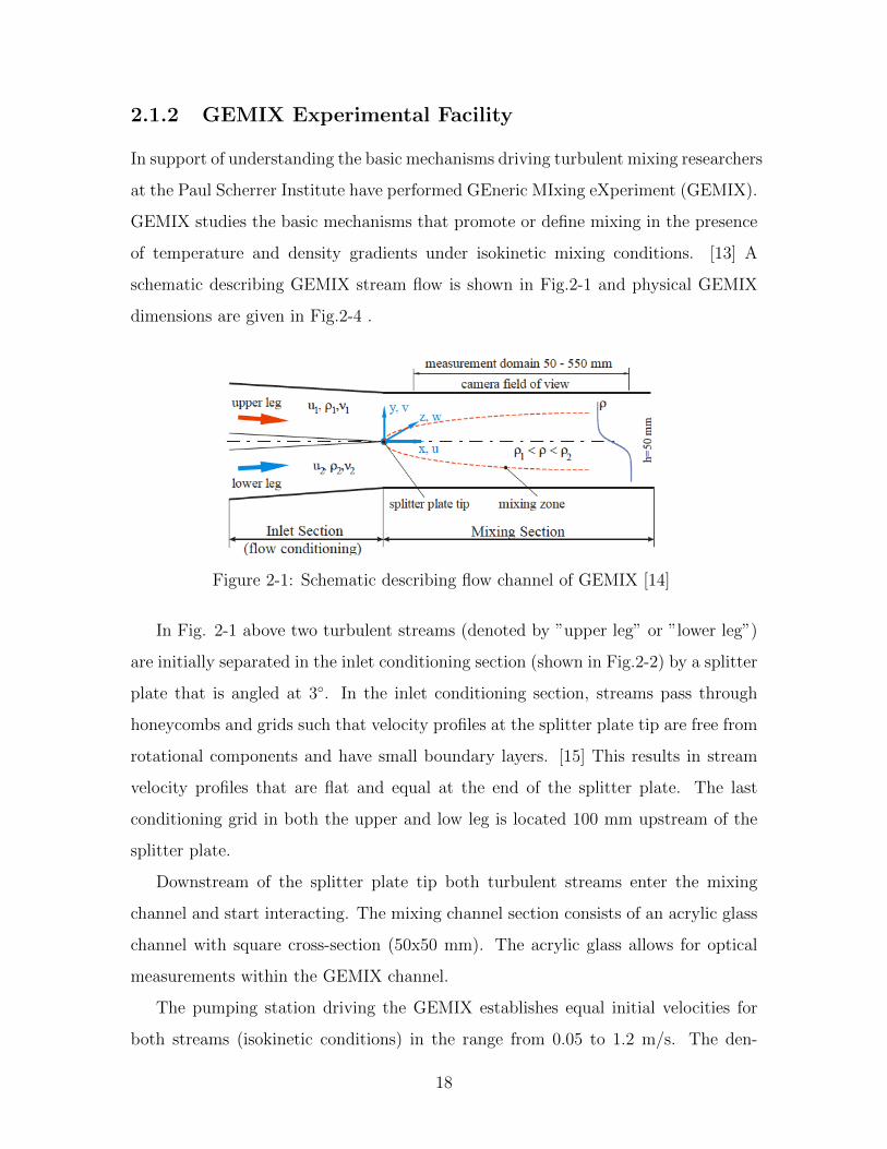
schematic describing GEMIX stream flow is shown in Fig.2-1 and physical GEMIX
dimensions are given in Fig.2-4 .
Figure 2-1: Schematic describing flow channel of GEMIX [14]
In Fig. 2-1 above two turbulent streams (denoted by ”upper leg” or ”lower leg”)
are initially separated in the inlet conditioning section (shown in Fig.2-2) by a splitter
plate that is angled at 3◦. In the inlet conditioning section, streams pass through
honeycombs and grids such that velocity profiles at the splitter plate tip are free from
rotational components and have small boundary layers. [15] This results in stream
velocity profiles that are flat and equal at the end of the splitter plate. The last
conditioning grid in both the upper and low leg is located 100 mm upstream of the
splitter plate.
Downstream of the splitter plate tip both turbulent streams enter the mixing
channel and start interacting. The mixing channel section consists of an acrylic glass
channel with square cross-section (50x50 mm). The acrylic glass allows for optical
measurements within the GEMIX channel.
The pumping station driving the GEMIX establishes equal initial velocities for
both streams (isokinetic conditions) in the range from 0.05 to 1.2 m/s. The den-
18
Page 19
Figure 2-2: Inflow Condition of the GEMIX [14]
Figure 2-3: Mixing Channel of the GEMIX [14]
sity ρ, and the kinematic viscosity of both streams, ν, are adjusted by varying the
temperature and/or adding sucrose to the fluid in one leg to increase the density
difference. Density differences of up to 1.5% are achieved by heating one of the fluids.
For density differences above 1.5% sucrose is added. The fluid used in each leg is
either conductive tap water or non-conductive distilled water.
Full operating specifications for GEMIX is presented in Table 2.1 below. More
background on GEMIX set up can be found in [7], [14], and [15].
19
Page 20
Parameter Value
Density Difference (∆ρ) 0 %— 10%Reynolds number (Re) 2,500 — 60,000
Stream Velocity (u) 0.05 — 1.20 m/sStream Temperature Difference (∆T ) 0K — 50K
Table 2.1: GEMIX parameter operating range [16] [15]
Figure 2-4: Schematic describing dimensions of the GEMIX [7]
2.1.3 Measurement Methodology in GEMIX
The experimental measurement domain for GEMIX covers a range of x = 50mm
and x = 550mm downstream from the splitter plate tip (with respect to grid sys-
tem defined in Fig. 2-4.) Development of the velocity field and concentration field
downstream of the splitter plate is observed in the measurement domain using three
different flow measurement techniques; Particle Image Velocimetry(PIV), Wire-Mesh
sensors (WMS), and Laser Induced Fluorescence (LIF).
Partilce Image Velocimetry (PIV)
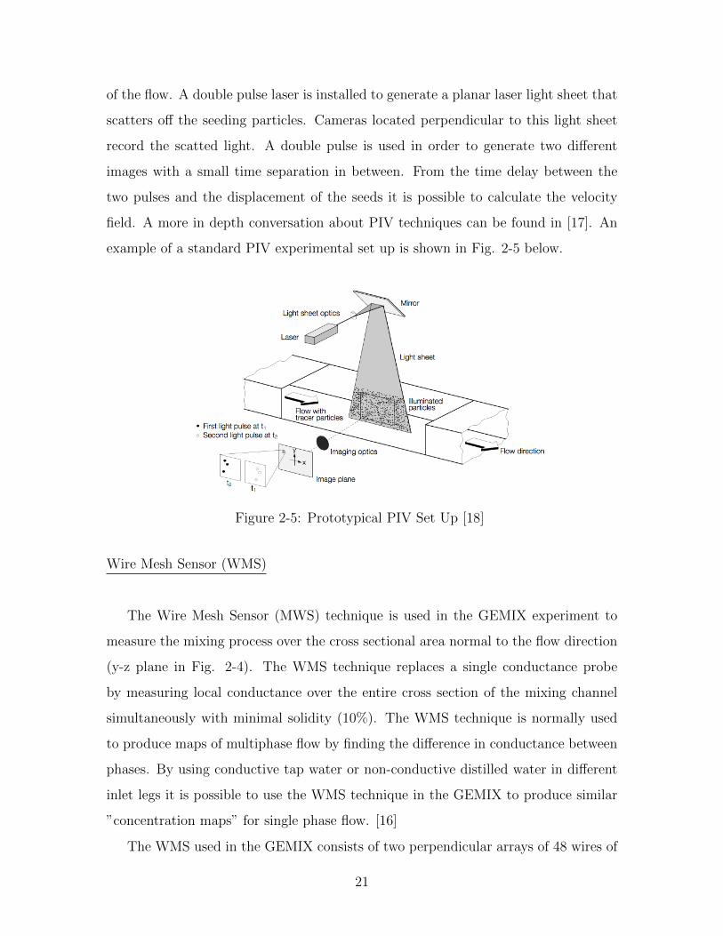
Particle Image Velocimetry (PIV) is employed to evaluate the instantaneous flow
velocity field in x-y plane of the GEMIX. [7] To start a PIV experiment small seeding
particles are injected into the flow of the experiment. These small particles are tiny,
neutrally buoyant and they can either be an aerosol or a solid depending on the nature
20
Page 21
of the flow. A double pulse laser is installed to generate a planar laser light sheet that
scatters off the seeding particles. Cameras located perpendicular to this light sheet
record the scatted light. A double pulse is used in order to generate two different
images with a small time separation in between. From the time delay between the
two pulses and the displacement of the seeds it is possible to calculate the velocity
field. A more in depth conversation about PIV techniques can be found in [17]. An
example of a standard PIV experimental set up is shown in Fig. 2-5 below.
Figure 2-5: Prototypical PIV Set Up [18]
Wire Mesh Sensor (WMS)
The Wire Mesh Sensor (MWS) technique is used in the GEMIX experiment to
measure the mixing process over the cross sectional area normal to the flow direction
(y-z plane in Fig. 2-4). The WMS technique replaces a single conductance probe
by measuring local conductance over the entire cross section of the mixing channel
simultaneously with minimal solidity (10%). The WMS technique is normally used
to produce maps of multiphase flow by finding the difference in conductance between
phases. By using conductive tap water or non-conductive distilled water in different
inlet legs it is possible to use the WMS technique in the GEMIX to produce similar
”concentration maps” for single phase flow. [16]
The WMS used in the GEMIX consists of two perpendicular arrays of 48 wires of
21
Page 22
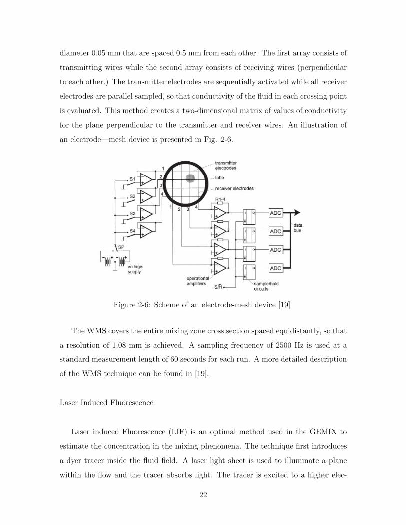
diameter 0.05 mm that are spaced 0.5 mm from each other. The first array consists of
transmitting wires while the second array consists of receiving wires (perpendicular
to each other.) The transmitter electrodes are sequentially activated while all receiver
electrodes are parallel sampled, so that conductivity of the fluid in each crossing point
is evaluated. This method creates a two-dimensional matrix of values of conductivity
for the plane perpendicular to the transmitter and receiver wires. An illustration of
an electrode—mesh device is presented in Fig. 2-6.
Figure 2-6: Scheme of an electrode-mesh device [19]
The WMS covers the entire mixing zone cross section spaced equidistantly, so that
a resolution of 1.08 mm is achieved. A sampling frequency of 2500 Hz is used at a
standard measurement length of 60 seconds for each run. A more detailed description
of the WMS technique can be found in [19].
Laser Induced Fluorescence
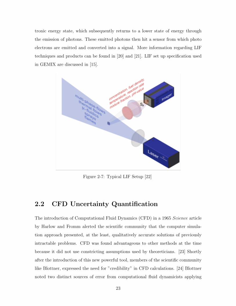
Laser induced Fluorescence (LIF) is an optimal method used in the GEMIX to
estimate the concentration in the mixing phenomena. The technique first introduces
a dyer tracer inside the fluid field. A laser light sheet is used to illuminate a plane
within the flow and the tracer absorbs light. The tracer is excited to a higher elec-
22
Page 23
tronic energy state, which subsequently returns to a lower state of energy through
the emission of photons. These emitted photons then hit a sensor from which photo
electrons are emitted and converted into a signal. More information regarding LIF
techniques and products can be found in [20] and [21]. LIF set up specification used
in GEMIX are discussed in [15].
Figure 2-7: Typical LIF Setup [22]
2.2 CFD Uncertainty Quantification
The introduction of Computational Fluid Dynamics (CFD) in a 1965 Science article
by Harlow and Fromm alerted the scientific community that the computer simula-
tion approach presented, at the least, qualitatively accurate solutions of previously
intractable problems. CFD was found advantageous to other methods at the time
because it did not use constricting assumptions used by theoreticians. [23] Shortly
after the introduction of this new powerful tool, members of the scientific community
like Blottner, expressed the need for ”credibility” in CFD calculations. [24] Blottner
noted two distinct sources of error from computational fluid dynamicists applying
23
Page 24
inappropriate governing equations or using inaccurate solution procedures. It was in
1986 that the ASME Journal of Fluids Engineering formally announced the need for
”verification and validation” in the policy statement below: [25]:
The Journal of Fluids Engineering will not accept for publication any paper re-
porting the numerical solutions of a fluids engineering problem that fails to address
the task systematic truncation error testing and accuracy estimation
The difficulty in obtaining reliable CFD results is in part because CFD is a knowl-
edge based activity, and despite CFD software being available, the knowledge known
by expert users is not always available. This has led to a number of initiatives in the
scientific community to develop ”standard best practices” for verifying and validating
CFD calculations. Notable examples include the BPGs developed by the European
Research Community on Flow, Turbulence, and Combustion (ERCOFTAC); the Eu-
ropean Thematic Network for Quality and Trust in the Industrial Application of CFD
(QNET-CFD); the Organization for Economic Co-operation and Development /Nu-
clear Energy Agency/Committee on the Safety of Nuclear Installations CFD working
groups; and the American Society of Mechanical Engineers (ASME), ”Standard for
Verification and Validation in Computational Fluid Dynamics and Heat Transfer.”
[26] [27] [28] [6]
The focus of this study is to evaluate the applicability, capabilities and limitations
of the ASME proposed V&V20 on high quality, CFD grade GEMIX data, for which a
UQ study has been previously performed with Polynomial Chaos Expansion (PCE).
[6] [7] PCE is an uncertainty propagation method that uses stochastic variables in
a mathematical series form to estimate the probability density function (PDF) of a
system response. PCE has advantages among other UQ methods (such as Monte
Carlo) as it uses a significantly smaller number of sampling points for multivariate
models; thus reducing computational expenses. PCE, although not the primary focus
of this study, serves as point a reference when assessing the proposed ASME V&V20
standard.
24
Page 25
2.2.1 ASME V&V20
The primary objective of the ASME verification and validation (V&V) 20 document is
to provide a standard for quantifying model uncertainty computed from the compari-
son of solution and experimental data for a specified variable at a specified validation
point. The following sections will lay out the fundamental nomenclature, equations,
and methods necessary for the ASME V&V20 validation approach.
Errors and Uncertainties
The ASME V&V20 standard uses the following definitions:
(1) error (of measurement), δ : ”result of a measurement minus a true value of the
measurand” [29]
(2) uncertainty (of measurement), u : ”parameter, associated with the result of a
measurement, that characterizes the dispersion of the values that could reasonably
be attributed to the measurand ” [29]
Under these definitions, an error, δ, is a quantity that has a particular sign and
magnitude, and a specific error, δi, is the difference caused by an error source i be-
tween a quantity (measured or simulated) and its true value. Error whose sign and
magnitude is known is assumed to be removed by correction in this standard. Thus,
any remaining error is said to be of unknown sign and magnitude, and uncertainty,
u, is estimated with the assumption that, ±u, characterizes the range containing δ.
Validation Approach
The ASME V&V20 validation process compares a simulation result (solution) and
an experimental result (data) for specified variables under certain conditions in order
to quantify the degree to which a model is an accurate representation of the real world
25
Page 26
from the perspective of the intended uses of the model (put simply, the quantifying
error in the model δmodel). To start the validation approach, denote the predicted
value — of a variable of interest U— from a simulation solution as S, the value
determined from experimental data as D, and the true value as T . The validation
comparison error, E, is defined as the difference between the solution value (S) and
the experimental value (D).
E = S −D (2.1)
The error in the solution value, S, is defined as the difference between S and the true
value T .
δS = S − T (2.2)
Similarly, the error in the experimental value, D, is defined as the difference between
D and the true value T .
δD = D − T (2.3)
Using Eq. 2.1, Eq. 2.2, and Eq. 2.3 the validation error, E, is expressed as
E = S −D = (T + δS) = (T + δD) = δS − δD (2.4)
Thus, the validation comparison error E is the difference of all errors in the simulation
result and the experimental result, and its sign and magnitude are known once S and
D are determined.
Errors in the predicted simulation result, S, can be assigned to three categories:
(a) the error δmodel due to modeling assumptions and approximations.
(b) the error δnum due to the numerical solution of the equations.
(c) the error δinput in the simulation result due to errors in the simulation input
parameter.
The total simulation error, δS, is summation of the three errors aforementioned
26
Page 27
above.
δS = δmodel + δnum + δinput (2.5)
The objective of the validation exercise, however, is to estimate δmodel within an
uncertainty range. Using Eq. 2.4 and Eq. 2.5, δmodel is defined as
δmodel = E − (δnum + δinput − δD) (2.6)
Under the assumption that S and D have been determined, the sign and magnitude
of E are known from Eq. 2.1. However, the magnitudes and signs of δnum, δinput, and
δD are still unknown.
It is noted in the ASME standard that once S and D have been determined, their
values will always differ by an equivalent fixed amount from the true value T . Thus,
all errors affecting S and D are considered to be ”fossilized” [30] and δnum, δinput,
δmodel, and δD are all considered systematic errors. This indicates that unum, uinput,
and uD are systematic uncertainties associated with the aforementioned systematic
errors δ. Under the ISO guidelines [31], there is no distinction made mathematically
between uncertainties defined as ”systematic” and ”random.” A systematic error is a
single realization from a parent population of possible values from a systematic error
source, and the corresponding systematic uncertainty, u, is the estimated standard
deviation of that parent population.
Applying the mathematical definitions of systematic error and uncertainty, a vali-
dation standard uncertainty, uval, is defined as the estimate of the standard deviation
of the parent population of combined errors (δnum + δinput − δD). Where, if all three
errors are effectively independent, uval is expressed as
uval =√u2num + u2input − u2D (2.7)
Using the relationship shown in Eq. 2.6 and Eq. 2.7,
E ± uval (2.8)
27
Page 28
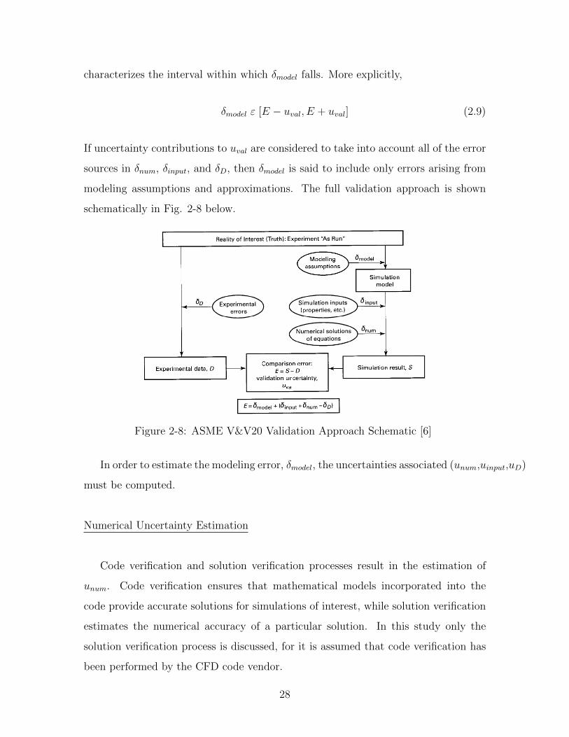
characterizes the interval within which δmodel falls. More explicitly,
δmodel ε [E − uval, E + uval] (2.9)
If uncertainty contributions to uval are considered to take into account all of the error
sources in δnum, δinput, and δD, then δmodel is said to include only errors arising from
modeling assumptions and approximations. The full validation approach is shown
schematically in Fig. 2-8 below.
Figure 2-8: ASME V&V20 Validation Approach Schematic [6]
In order to estimate the modeling error, δmodel, the uncertainties associated (unum,uinput,uD)
must be computed.
Numerical Uncertainty Estimation
Code verification and solution verification processes result in the estimation of
unum. Code verification ensures that mathematical models incorporated into the
code provide accurate solutions for simulations of interest, while solution verification
estimates the numerical accuracy of a particular solution. In this study only the
solution verification process is discussed, for it is assumed that code verification has
been performed by the CFD code vendor.
28
Page 29
In solution verification, error and uncertainty estimates are similar, but not equiv-
alent calculations. Error estimates are used to provide an improvement in a certain
calculation, while uncertainty estimations are intended to provide ”banding” of nu-
merical error in a certain calculation. For example, if the calculation for flow velocity
using a particular grid is v and the associated error estimate is ε, then the ”improved”
value (closer to the true value vT ) will be (v − ε). In contrast, the uncertainty es-
timate, Up%, is used to provide an interval (v ± Up%) that characterizes the range
within which the true value vT falls with a probability of p%. A common uncertainty
target is to estimate the uncertainty band with a probability of 95% (similar to the
2σ confidence intervals used in Gaussian distribution).
The solution verification process starts with the estimation of numerical error.
Systematic grid refinement studies are commonly used in solution verification pro-
cesses to estimate this ”error.” One of the most popular approaches to estimate error
is the Richardson Extrapolation Method. [32] [33]
Richardson Extrapolation (RE) assumes that discrete solutions, f , have a series
representation in the grid spacing h (or ∆) of
f = fexact + g1h+ g2h2 + g3h
3 + ... (2.10)
The functions g1, g2, etc. are defined in the continuum and do not depend on any
discretization For second order methods, g1 = 0. The concept is then to combine
two separate discrete solutions f1 and f2 on two different grids with uniform discrete
spacings of h1 (finer grid) and h2 (coarser grid) in order to solve for g2 at the grid
points in Eq. 2.10 and then obtain a more accurate estimation of fexact. The result
is expressed in the following equation[33]:
fexact =h22f1 − h21f2h22 − h21
+H.O.T. (2.11)
In the expression above H.O.T. are higher order terms. If a grid refinement ratio
r = h2h1
is defined, then Eq. 2.11 can be expressed as the correction to the fine grid
29
Page 30
solution f1 and the H.O.T are dropped. [34]
fexact u f1 +f1 − f2r2 − 1
(2.12)
Grid doubling is often associated with RE, however, it is not required and the grid
ratio may be any real number. The grid ratio does not have to be an integer, but a
ratio greater than 1.3 is recommended for practical problems. [6]
Eq. 2.12 is considered to be 4th order accurate if f1 and f2 are 2nd order accurate,
however, this is only true if odd powers are absent in the expansion shown in Eq. 2.10.
In derivation above, Richardson managed to remove odd powers in the expansion by
using a 2nd order centered difference schemes. If uncentered differences are used,
such as the upstream weighting of advection terms, even if the methods are second
order, the RE extrapolation is 3rd order accurate. [34]
Without assuming the absence of odd powers in Eq. 2.10, the equation above (Eq.
2.12) can be further generalized [35] to p-th order methods and r-value of grid ratio.
fexact u f1 +f1 − f2rp − 1
(2.13)
Eq. 2.13 is a p +2 order (central difference scheme) accurate error estimator of the
fine grid solution. The estimated fractional error E1 for the fine grid solution f1 is
thus
E1[FineGrid] =ε
rp − 1(2.14)
Where,
ε =f2 − f1f1
(2.15)
The error estimator E1 itself does not provide a very good confidence interval, and is
certainly not a bound on error. However, within the CFD community there exists a
practical confidence level for the ε in Eq. 2.15 obtained using a grid doubling and a
verified second order accuracy code.
Prior to the Richardson Extrapolation being performed to estimate error, it is
recommended that iterative convergence be achieved. Iterative error can cause noise
30
Page 31
in the proceeding the uncertainty estimation process, especially since RE amplifies
iterative error.[34] The common rule of thumb for iterative error — although not
necessarily justified [6] — is to require at least three orders of magnitude decrease
in properly normalized residuals for each equation solved over the computational
domain. Potential methods for quantifying iterative uncertainty have been suggested
by Ferziger in [36] and referenced by the ASME in [37].
If the uncertainty contributed by estimated iterative error is much less than the
uncertainty contributed by the discretization error, then we take the numerical un-
certainty to be equivalent to the uncertainty caused by discretization error.
unum = uh (2.16)
Otherwise, the two sources of uncertainty must be combined.
unum = uh + uiter (2.17)
To estimate the numerical uncertainty associated with the discretization error of
the fine grid, E1, the Grid Convergence Index (GCI) methodology is applied. The
concept is to use GCI to approximately relate ε of Eq. 2.15 — obtained using any
grid convergence study performed (order p and grid ratio r) — to the ε that would be
expected from a grid convergence study of the same problem with the fine grid using
p = 2 and r = 2. Essentially, the GCI relates the results from any grid refinement
test to the expected results from a grid doubling using a second-order method. GCI
is expressed below in Eq. 2.18.
GCI[FineGrid] = Fs|ε|
rp − 1, Fs = 3 (2.18)
It should be noted that for a grid doubling (r=2) with a second order method (p=2)
we obtain that GCI = |ε|, as intended by the initial definition of GCI. In Eq. 2.18 Fs
is defined as the ”factor of safety” over the RE estimator E1. The use of Fs = 3 is
meant to make grid doubling with second order methods the standard or comparison.
31
Page 32
A safety factor of Fs = 3 has been recommended for two-grid convergence studies,
but a safety factor of Fs = 1.25 is a less overly conservative choice for convergence
studies with a minimum of three grids to experimentally demonstrate the observed
order of convergence p on the actual problem. A more detailed discussion on the use
of safety factors can be found in [34].
The recommended procedure for performing a GCI estimation is presented below:
[37] [6]
(1) Define a representative cell, mesh, or grid size h. For example, for three-
dimensional calculations.
h =
[1
N
N∑i=1
(∆Vi)
]1/3(2.19)
For two dimensional calculations,
h =
[1
N
N∑i=1
(∆Ai)
]1/2(2.20)
Where ∆Vi is the volume, ∆Ai is the area of the i-th cell, and N is the total number
of cells used for the computations.
(2) Select three significantly different sets of grids and run simulations to deter-
mine the values of key variables important to the objective of the simulation study
(φ). It is desirable that the grid refinement factor r = hcoarse/hfine be greater than
1.3. The grid refinement, however, be done systematically, that is, the refinement
itself should be structured even if the grid is unstructured. It is highly recommended
not use grid refinement ratios (rx = 1.2, ry = 1.5) in different directions because er-
roneous observed p values are produced. Geometrically similar cells are required in
order to prevent noisy and incorrect p values.
(3) Let h1, h2, h3 and r21 = h2/h1, r32 = h3/h2, and calculate the apparent order
32
Page 33
p of the method using the expressions below
p =1
ln(r21)|ln|ε32/ε21|+ q(p)| (2.21)
q(p) = ln
(rp21 − srp32 − s
)(2.22)
s = 1 · sgn(ε32/ε21) (2.23)
Where ε32 = φ3−φ2, ε21 = φ2−φ1 and φk denotes the soltuion in the k-th grid. Note
that q(p) = 0 for r21 = r32. Eq. 2.21 can be solved using fixed-point iteration with
the initial guess equal to the first term.
(4) Calculate the extrapolated values from
φ21ext = (rp21φ1 − φ2)/(r
p21 − 1) (2.24)
Similarly calculate φ32ext.
(5) Calculate and report the following error estimates, along with the apparent
order p
Approximate relative error:
ε21a =
∣∣∣∣φ1 − φ2
φ1
∣∣∣∣ (2.25)
Extrapolated relative error:
ε21ext =
∣∣∣∣φ12ext − φ1
φ12ext
∣∣∣∣ (2.26)
Grid Convergence Index:
GCI21Fine =1.25e21arp21 − 1
(2.27)
33
Page 34
In order to agree with the international standard use of one standard deviation 1σ,
this ASME standard developed Eq. 2.7 using the 1σ standard and the corresponding
uncertainty unum. If the procedure adopted for other uncertainty components is
to base everything on the expanded uncertainty U95%, then Unum = GCI and no
statistical assumption for the distribution is required. Otherwise to convert GCI
from Unum to the unum needed in Eq. 2.7 it will be necessary to make an assumption.
If the error distribution is Gaussian about the fine grid solution, the value of unum
would be obtained by using an expansion factor of k = 2.
unum = Unum/k = GCI/2 (2.28)
For poorly behaved problems (oscillatory convergence), the error distribution about
the fine grid is roughly Gaussian. For well behaved and highly resolved problems
the error distribution is roughly Gaussian about the extrapolated solution φ21ext found
in Eq. 2.24. Thus the error distribution about the fine solution becomes a shift
Gaussian. Conservative analysis of unum for this case suggests an expansion factor of
k = 1.5.
Input Uncertainty Estimation
Computational simulations contain experimentally determined parameters that
have a certain uncertainty associated with them. These uncertainties propagate
through the model of the system being assessed. A pipe flow example would be
estimating the uncertainty in the friction coefficient given uncertainty in flow veloc-
ity measurements. In the ASME V&V20 standard a global and local method for
quantifying input uncertainty is presented. This section discusses the local approach
suggested in the standard for estimating input uncertainty uinput.
The the sensitivity coefficient method takes a local view for uncertainty estima-
tion. This method analyzes the response of the system in a small neighborhood of
the nominal parameter vector. Using a linear Taylor series expansion in parameter
space, the input uncertainty propagation equation for a simulation result S with n
34
Page 35
uncorrelated random input parameters is expressed as
u2input =n∑i=1
(δS
δXi
uXi
)2
(2.29)
where S is the simulation result (either a point value or integral quantity ), Xi is the
input parameter, and uXi is the corresponding standard uncertainty in parameter Xi.
The partial derivatives, δS/δXi, are called sensitivity coefficients of the simulation
result S with respect to input parameter Xi.
In order to calculate the parameter input uncertainty the sensitivity coefficients
must be solved for. The method to compute the sensitivity coefficient begins by run-
ning a simulation with nominal values of the parameter vector X. A second simulation
is run with a perturbed value (Xi + ∆Xi ) for input parameter Xi. The sensitivity
coefficient is then computed using a second order finite difference approximation in
the parameter space.
δS
δXi
=S(X1, X2, . . . , Xi + ∆X, . . . , Xn)− S(X1, X2, . . . , Xi −∆Xi, . . . , Xn)
2∆Xi
+O(∆X2i )
(2.30)
Using this method 2n +1 simulations will be required to compute n second order
sensitivity coefficients. One of the challenges associated with this method is selecting
an appropriate perturbation size ∆Xi. If ∆Xi is too large then truncation errors in
Eq. 2.30 will be too large. If ∆Xi is too small then machine round off errors become
significant. Numerical experimentation is recommended when using this method.
Experimental Uncertainty
Experimental uncertainty analysis is used to determine the uncertainty estimate
uD. The process for experimental uncertainty analysis is to calculate the uncertainties
of individual measured variables and to use those uncertainties to estimate the uncer-
tainty of the experimental solution, D, derived from those variables.This study does
not have access to the GEMIX experimental uncertainties, thus the full ASME valida-
tion study cannot completed. This study will instead focus on analyzing the GEMIX
35
Page 36
simulation solution uncertainty. For a full explanation on experimental uncertainty
analysis reference [6], [38], and [39].
2.2.2 Polynomial Chaos Expansion Theory
Polynomial Chaos Expansion (PCE) method is based on spectral representation of
uncertainty using orthogonal polynomials The PCE method consists of projecting the
output of a model onto a basis of orthogonal stochastic polynomials with a set of ran-
dom input variables. This stochastic projection provides a convenient representation
of model output variability with respect to the set of random input variables. The
model response is expressed as
R(ξ) =inf∑k=0
ckψk(ξ) (2.31)
where ψk are selected orthogonal basis of the random variables (ξ) and ck are the
deterministic coefficients. The computation of coefficients ck allow for the estimation
of the response R. A Sobol Decomposition method can be used on this PCE model
response to obtain Sobol indices that represent the effect of each input parameter on
the output parameter.
The full mathematical description of the PCE and Sobol decomposition method is
outside the scope of this study. Instead, this study will focus on comparing GEMIX
simulation sobol indices computed using a PCE study [7] with the sensitivity coef-
ficients computed in this study using the ASME V&V20 methodology. This study
aims at highlighting the discrepancies between the two methodologies for computing
sensitivity indices.
36
Page 37
Chapter 3
Computational Methods, Results,
and Discussion
3.1 MIT GEMIX Simulation
3.1.1 Geometry, Mesh, and Models
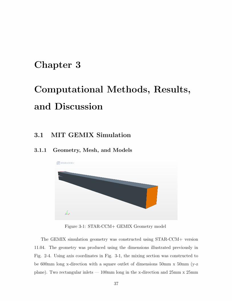
Figure 3-1: STAR-CCM+ GEMIX Geometry model
The GEMIX simulation geometry was constructed using STAR-CCM+ version
11.04. The geometry was produced using the dimensions illustrated previously in
Fig. 2-4. Using axis coordinates in Fig. 3-1, the mixing section was constructed to
be 600mm long x-direction with a square outlet of dimensions 50mm x 50mm (y-z
plane). Two rectangular inlets — 100mm long in the x-direction and 25mm x 25mm
37
Page 38
in the y-z plane— are connected to the mixing section at a three degree angle (splitter
plate).
Figure 3-2: Computational mesh used to construct STAR-CCM+ simulation model[40]
The computational mesh for this simulation was constructed using the direct
mesher in STAR-CCM+. A quadrilateral mesher was used to produce a uniform
mesh with 100 nodes in the x-direction and 30 nodes in the z-direction. Additional
refinement in the y-axis was introduced to capture turbulent mixing phenomenon that
occurred in the center of the mixing channel. To produce this additional refinement,
a prism layer method with a hyperbolic tangent stretching function was employed.
Using a prism layer stretching factor of 1.5, the refinement in the y-axis becomes
finer as the mesh approaches the center) of the mixing section. The final grid used
contains 432,000 cells. The final simulation mesh used in this study is presented in
3-3.
The simulation uses steady state and incompressible flow conditions. To reduce
computational time, a segregated flow model was used. The segregated flow model in
STAR-CCM+ uses a 2nd-Order upwind scheme as the discretization scheme. A multi-
component liquid non reacting model was employed to capture the concentration of
mixing between the lower and upper inlet fluid streams. Water at a temperature of
23oC and a density of 992kg/m3 was considered at both legs. The boundary layer of
the splitter was resolved with a low Reynolds k-e model, while adopting an all y+
model for all other wall boundaries.
38
Page 39
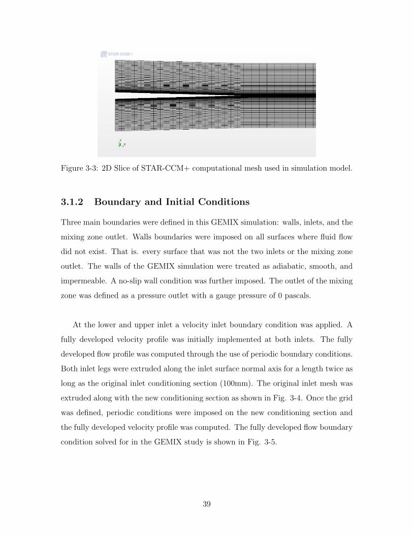
Figure 3-3: 2D Slice of STAR-CCM+ computational mesh used in simulation model.
3.1.2 Boundary and Initial Conditions
Three main boundaries were defined in this GEMIX simulation: walls, inlets, and the
mixing zone outlet. Walls boundaries were imposed on all surfaces where fluid flow
did not exist. That is. every surface that was not the two inlets or the mixing zone
outlet. The walls of the GEMIX simulation were treated as adiabatic, smooth, and
impermeable. A no-slip wall condition was further imposed. The outlet of the mixing
zone was defined as a pressure outlet with a gauge pressure of 0 pascals.
At the lower and upper inlet a velocity inlet boundary condition was applied. A
fully developed velocity profile was initially implemented at both inlets. The fully
developed flow profile was computed through the use of periodic boundary conditions.
Both inlet legs were extruded along the inlet surface normal axis for a length twice as
long as the original inlet conditioning section (100mm). The original inlet mesh was
extruded along with the new conditioning section as shown in Fig. 3-4. Once the grid
was defined, periodic conditions were imposed on the new conditioning section and
the fully developed velocity profile was computed. The fully developed flow boundary
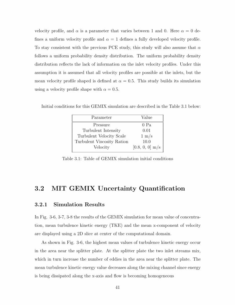
condition solved for in the GEMIX study is shown in Fig. 3-5.
39
Page 40
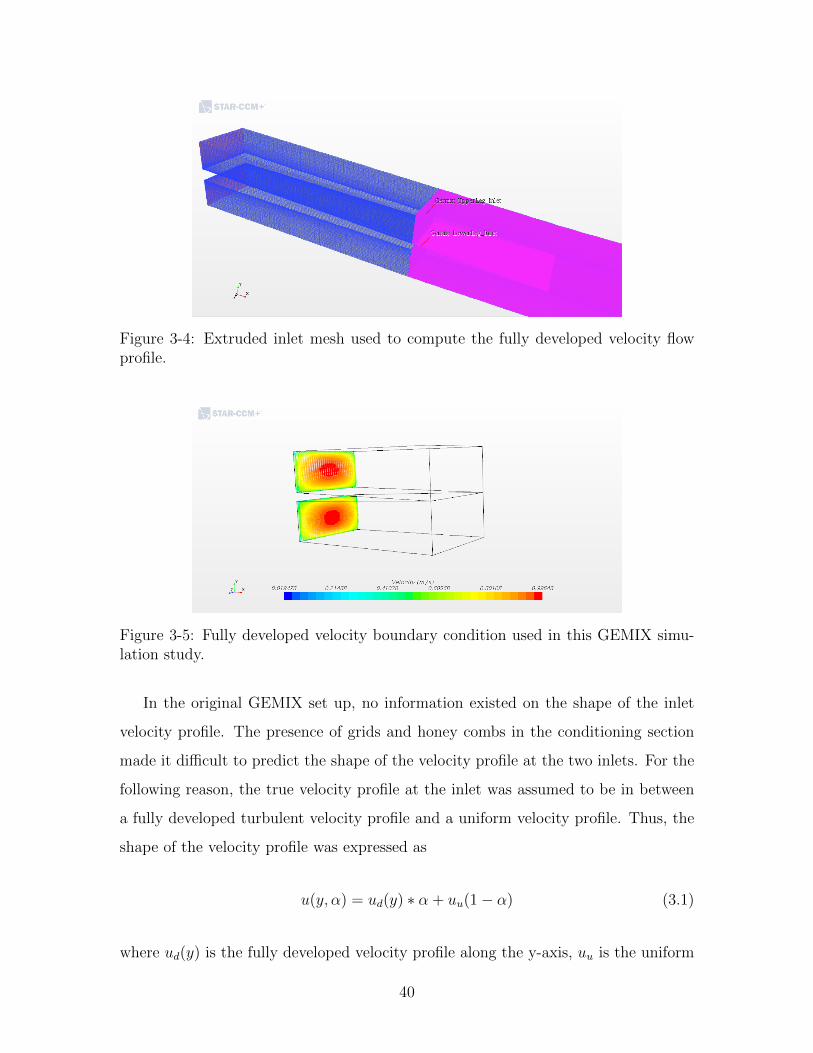
Figure 3-4: Extruded inlet mesh used to compute the fully developed velocity flowprofile.
Figure 3-5: Fully developed velocity boundary condition used in this GEMIX simu-lation study.
In the original GEMIX set up, no information existed on the shape of the inlet
velocity profile. The presence of grids and honey combs in the conditioning section
made it difficult to predict the shape of the velocity profile at the two inlets. For the
following reason, the true velocity profile at the inlet was assumed to be in between
a fully developed turbulent velocity profile and a uniform velocity profile. Thus, the
shape of the velocity profile was expressed as
u(y, α) = ud(y) ∗ α + uu(1− α) (3.1)
where ud(y) is the fully developed velocity profile along the y-axis, uu is the uniform
40
Page 41
velocity profile, and α is a parameter that varies between 1 and 0. Here α = 0 de-
fines a uniform velocity profile and α = 1 defines a fully developed velocity profile.
To stay consistent with the previous PCE study, this study will also assume that α
follows a uniform probability density distribution. The uniform probability density
distribution reflects the lack of information on the inlet velocity profiles. Under this
assumption it is assumed that all velocity profiles are possible at the inlets, but the
mean velocity profile shaped is defined at α = 0.5. This study builds its simulation
using a velocity profile shape with α = 0.5.
Initial conditions for this GEMIX simulation are described in the Table 3.1 below:
Parameter Value
Pressure 0 PaTurbulent Intensity 0.01
Turbulent Velocity Scale 1 m/sTurbulent Viscosity Ration 10.0
Velocity [0.8, 0, 0] m/s
Table 3.1: Table of GEMIX simulation initial conditions
3.2 MIT GEMIX Uncertainty Quantification
3.2.1 Simulation Results
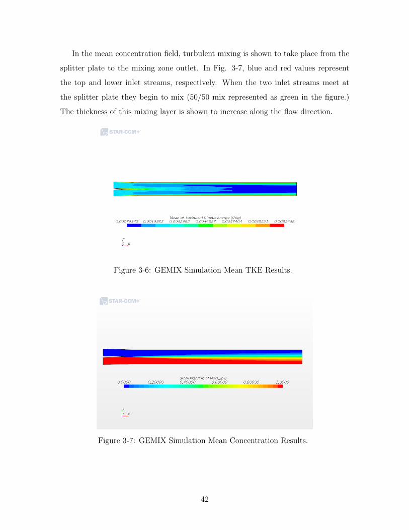
In Fig. 3-6, 3-7, 3-8 the results of the GEMIX simulation for mean value of concentra-
tion, mean turbulence kinetic energy (TKE) and the mean x-component of velocity
are displayed using a 2D slice at center of the computational domain.
As shown in Fig. 3-6, the highest mean values of turbulence kinetic energy occur
in the area near the splitter plate. At the splitter plate the two inlet streams mix,
which in turn increase the number of eddies in the area near the splitter plate. The
mean turbulence kinetic energy value decreases along the mixing channel since energy
is being dissipated along the x-axis and flow is becoming homogeneous
41
Page 42
In the mean concentration field, turbulent mixing is shown to take place from the
splitter plate to the mixing zone outlet. In Fig. 3-7, blue and red values represent
the top and lower inlet streams, respectively. When the two inlet streams meet at
the splitter plate they begin to mix (50/50 mix represented as green in the figure.)
The thickness of this mixing layer is shown to increase along the flow direction.
Figure 3-6: GEMIX Simulation Mean TKE Results.
Figure 3-7: GEMIX Simulation Mean Concentration Results.
42
Page 43
Figure 3-8: GEMIX Simulation Mean Velocity [x-component] Results.
In Fig. 3-9, 3-10, and 3-11 the mean velocity, mean TKE, and mean concentration
results of the GEMIX simulation are plotted against the experimental results of the
GEMIX facility and the mean polynomial chaos expansion (PCE) simulation values
produced in [7].
Figure 3-9: Mean Velocity [x] Results Comparison
43
Page 44
Figure 3-10: Mean TKE Results Comparison
Figure 3-11: Mean Concentration Results Comparison
44
Page 45
Simulation mean velocity and concentration profile results show agreement with
fluid physics, experimental results and mean PCE simulation results. The simulation
results in Fig. 3-9 show the mean velocity profile flatten downstream in the mixing
section 1, which is consistent with physical expectation of flow becoming more devel-
oped down stream. Discrepancies between the k-e model mean x-component velocity
results and the mean PCE velocity results at near walls can be attributed to the use
of wall functions.
The simulation mean TKE profile results fit the experimental measurements and
the mean PCE simulation results fairly well. At x=60mm and x=150mm, the simu-
lation mean TKE profile under predicts the experimental TKE peak at y=0mm. A
possible explanation for this discrepancy is in the use of the Reynolds average ap-
proach. Larger coherent eddy structures that appear near the splitter plate may not
be accounted for under the k-e model, thus the k-e model is under predicting the
turbulent kinetic energy that exists near the splitter plate. It should be noted that
experimental TKE measurements at x=450mm show larger TKE values than previ-
ous plane measurements. It is not necessarily clear whether the increase in TKE near
the outlet is a result of larger coherent structure or a measurement error. Further
experimental measurements near the outlet are required to assess this effect.
For the mean concentration profile, the GEMIX simulation results slightly over
predicts the experimentally measured thickness of the mixing layer near the splitter
plate. The k-e model occasionally over predicts the eddy viscosity, leading to a
slightly thicker mixing layer. Experimental concentration measurements using both
the Wire Mesh Sensors (WMS) and Laser Induced Fluorescence (LIF) are presented
alongside PCE and GEMIX simulation results in Fig. 3-11. Physically, the GEMIX
simulation mean concentration profile results show an increasing mixing layer moving
downstream which is expected.
1It should be noted that x=0mm is located at the splitter plate. Thus, x=60mm is the planeclosest to the splitter plate while x=450mm is the plane closest to the mixing section outlet. Movingdownstream is moving from x=60mm to x=450mm.
45
Page 46
3.2.2 Numerical Uncertainty
The first step to quantifying solution uncertainty is to solve for the numerical uncer-
tainty. In the ASME V&V20 standard, the two main sources of numerical uncertainty
are due to iterative convergence error and discretization error. Iterative convergence
error was confirmed to be negligible in this simulation; on the order of 10−7. Hence,
uncertainty due to discretization error is deemed to be equivalent to the numerical
uncertainty (Eq. 2.16).
The discretization study was performed on a 2D GEMIX simulation with varying
degrees of refinement along the y-axis. Specifications for the three grids can be found
in Table 3.2 below. Grid refinement along the x-axis is greater along the mixing section
(100 nodes) than the inlet legs (20 nodes). Mixing zone grid refinement along the
y-axis used a prism layer stretching factor of 1.5 and node dimensions along the x-axis
remained constant for all grids. A total grid refinement ratio of 1.414 was utilized.
A larger grid refinement ratio would require either additional y-axis refinement or
y-axis coarsening. Additional refinement along the y-axis would provide negligible
changes in solution value, providing little to no useful information. Coarsening the
grid further, say less than 30 cells along the y-axis,would result in the simulation no
longer capturing the mixing behavior near the splitter plate. As a result of these
constraints, the grid refinement ratio greater than 1.3 was determined to be optimal
for the study.
Using the following grids, a Richardson Extrapolation study — described in sec-
tion 2.2.1— was performed to determine the numerical uncertainty due to discretiza-
tion error. The results of the discretization study are presented in Fig. 3-12, Fig.
3-14, and Fig. 3-13.
Simulation X-Nodes Y-Nodes #Cells
A 20 100 120 14400B 20 100 60 7200C 20 100 30 3600
Table 3.2: Table of grid dimensions used in discretization study.
46
Page 47
Figure 3-12: Mean Concentration standard numerical uncertainty (unum)
Figure 3-13: Mean TKE standard numerical uncertainty (unum)
47
Page 48
Figure 3-14: Mean Velocity [x] standard numerical uncertainty (unum)
Numerical uncertainty due to discretization error is most dominant within the
concentration profile computations near the splitter plate and the edges of the mixing
layer. At x=150mm and y= -2.5mm the concentration profile numerical uncertainty is
the greatest, with the mean concentration uncertainty bound ranging±0.77. It should
be noted that this uncertainty measurement is overly conservative and unphysical
since the boundaries of mean concentration values are between 0 and 1. As the mixing
layer further develops downstream the uncertainties due to discretization decrease
along the center (y=0mm). Numerical uncertainty, however, increases near the edges
of the mixing layer. This is expected for as the mesh becomes coarser the mixing
layer becomes less pronounced. That is, the eddy viscosity is being averaged over
larger cells which artificially increase the size of the mixing layer.
Mean TKE profile computations show similar numerical uncertainty behavior near
the splitter plate, and additional discretization sensitivity near the walls of the mixing
section. At x-60mm discretization error near the splitter plate dominates, with a
maximum numerical uncertainty bound of ± 0.01 m2/s2 at y= ±5 mm. Similar to
the behavior shown in the mean concentration profiles, it is shown that discretization
error near the center of the mixing section decreases downstream. An exception to
48
Page 49
this behavior occurs at x=450mm with an unexpectedly large numerical uncertainty
near the outlet. A large numerical uncertainty for the TKE profile exists near the
walls of the mixing section. Further examining Fig. 3-6 shows a sharp TKE gradient
near the wall of the mixing section. This sharp gradient, resulting from the use of
wall functions, is likely the cause of the large numerical uncertainties shown near the
wall in Fig. 3-13.
On the contrast, mean x-component velocity profile computation is fairly insensi-
tive to discretization error. Discretization error near the outlet of the mixing section
is fairly low, varying on the order of 10−2 m/s at the largest. The single largest con-
tribution to numerical uncerntainty for the velocity profile occurs at x=150mm near
the y=±10mm. A deeper investigation at the Richardson extrapolation showed the
extrapolated value at these points equating to 0.28 m/s. These low velocity point
values can be attributed to the fact that applying the Richardson extrapolation meth-
ods require solutions to be sufficiently close to the asymptotic range. Fig. 3-15 below
shows that monotonic convergence condition is not reached for solutions of different
grid sizes.
Figure 3-15: Mean velocity values along the y-axis for different grid sizes
49
Page 50
One of the challenges using the Richardson extrapolation method is that often
solutions are far from the asymptotic range. More specifically, we note that the
observed order of convergence p is typically greater or less than the actual order p.
Second order discretization methods were used in this simple physics simulation, thus
the actual order p should be in theory 2. Very few observed order p values in this
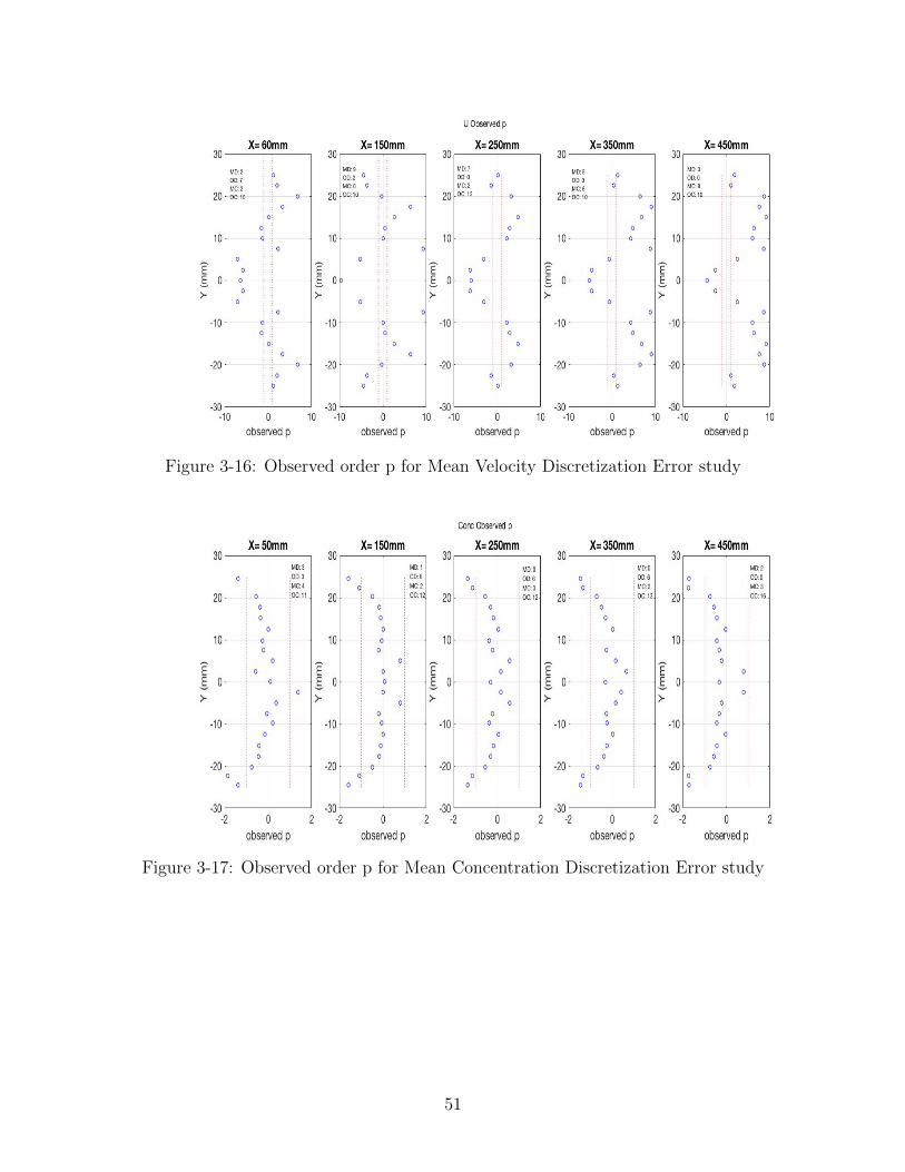
discretization study fall close to the actual order p. Fig. 3-16,3-18, and 3-17 showcase
the observed order p values over different positions on the y-axis. Included within
these figures are the number of instances of Monotonic Convergence (MC), Monotonic
Divergence (MD), Oscillatory Convergence (OC), and Oscillatory Divergence (OD).
In this turbulent mixing case, the non linearities in the mixing physics and in
gradient limiting became the dominant factor, producing non-monotonic convergence
behavior. In the figures below, the majority of computed p-value were either negative
or very close to zero. P-values that approach zero result in unrealistically large
discretization error estimates, while negative p-values are not useful. Conversely,
in certain circumstances (such as in 3-16) p-values approached large values such as
ten. Very large p-values such as these result in vanishingly small discretization errors.
The computed observed p-values demonstrate the difficulties associated with applying
the Richardson Extrapolation method to a turbulent case with non linear gradient
limiters and a small growth ratio.
50
Page 51
Figure 3-16: Observed order p for Mean Velocity Discretization Error study
Figure 3-17: Observed order p for Mean Concentration Discretization Error study
51
Page 52
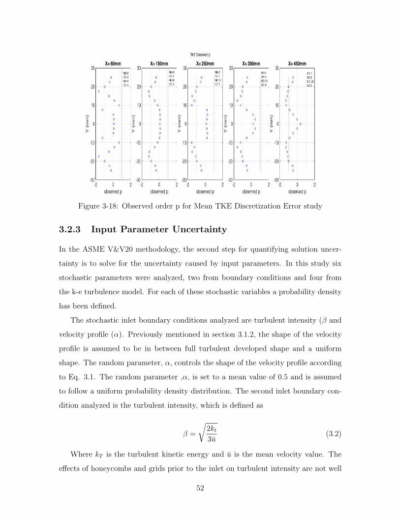
Figure 3-18: Observed order p for Mean TKE Discretization Error study
3.2.3 Input Parameter Uncertainty
In the ASME V&V20 methodology, the second step for quantifying solution uncer-
tainty is to solve for the uncertainty caused by input parameters. In this study six
stochastic parameters were analyzed, two from boundary conditions and four from
the k-e turbulence model. For each of these stochastic variables a probability density
has been defined.
The stochastic inlet boundary conditions analyzed are turbulent intensity (β and
velocity profile (α). Previously mentioned in section 3.1.2, the shape of the velocity
profile is assumed to be in between full turbulent developed shape and a uniform
shape. The random parameter, α, controls the shape of the velocity profile according
to Eq. 3.1. The random parameter ,α, is set to a mean value of 0.5 and is assumed
to follow a uniform probability density distribution. The second inlet boundary con-
dition analyzed is the turbulent intensity, which is defined as
β =
√2kt3u
(3.2)
Where kT is the turbulent kinetic energy and u is the mean velocity value. The
effects of honeycombs and grids prior to the inlet on turbulent intensity are not well
52
Page 53
known. For this reason, the turbulent intensity at the inlets has been defined as a
stochastic variable. Previous experimental studies used Eq. 3.3 to compute the mean
turbulent intensity at the inlet.
β = 0.16Re−1/8 (3.3)
Experimental results found the mean value of turbulent intensity to be 5%. [7] The
exact value of turbulent intensity at the inlet, however, is not known exactly. Thus, a
normal distribution was associated with the center mean value of turbulent intensity
(Using Eq. 3.3. The resulting standard deviation of this mean 1%.
The four other stochastic variables chosen were the empirical coefficients (Cµ, Cε2 , σk, σε)
used within the k-e model. Each of the coefficients will use their conventional values
as the center of the normal distributions and standard deviations for these empirical
coefficients were taken from [41]. When perturbing the values of the k-e coefficients
for the local sensitivity testing the following relations between model coefficients were
imposed. [42]
Cε1 =Cε22.1
+1.1
2.1(3.4)
σε =κ2√
Cµ(Cε2 − Cε1); κ = 0.4187 (3.5)
It should be noted that there are challenges associated with selecting k-e turbu-
lence model coefficients as stochastic variables for a local sensitivity study. The first
challenge is the fact that the k-e coefficients are empirically derived to get good agree-
ment with experimental results. If a k-e coefficient is perturbed in a sensitivity study
then one is no longer adhering to the particular conditions for which the coefficient
was computed. The second challenge is that by perturbing the k-e coefficients one is
implicitly stating that there is a correct k-e model, but the coefficients are incorrect.
Turbulence models and coefficients are derived for certain physical experiments, thus
altering the coefficients in a particular model for a different physical condition would
53
Page 54
not improve accuracy of the model. Finally, under the ASME V&V20 standard,
the computation of sensitivity coefficients rely on the fact that input parameters are
independently correlated. As shown in Eq. 3.5, σε is correlated to Cmu and Cε2 .
Nonetheless, this study will continue with the local sensitivity analysis of these k-e
coefficients in an effort to compare and contrast sensitivity coefficients produced in
the PCE study. [7]
In Table 3.3 below, the stochastic variables selected for the input parameter un-
certainty study are summarized. Along with each stochastic variable is a respective
probability density distribution and mean. The following distributions were selected
to match assumptions made in [7].
Stochastic Variable Probability Distribution Distribution Parameters
α Uniform µ = 0.5, σ = 8.33x10⁻²
β Normal µ = 0.05, σ = 0.01Cµ Normal µ = 0.09, σ = 2.4x10⁻³
Cεµ Normal µ = 1.92, σ = 1.174x10⁻¹
σκ Normal µ = 1.23, σ = 0.1661σε Normal µ = 0.7, σ = 0.1
Table 3.3: Table of Stochastic Variables and their respective probability density dis-tribution
Using the Table above, and Eq. 2.30, the sensitivity coefficients for the mean x-
component velocity, mean TKE, and mean concentration were solved. The sensitivity
coefficients profiles are displayed in Fig. 3-19, 3-20, and 3-21.
54
Page 55
Figure 3-19: Sensitivity Coefficients Mean TKE
Figure 3-20: Sensitivity Coefficients Mean Concentration
55
Page 56
Figure 3-21: Sensitivity Coefficients Mean Velocity
Upon computing the sensitivity coefficients, it is clear the two most dominant
input parameters for velocity, TKE, and concentration were the k-e coefficient Cµ
and inlet turbulent intensity (β). The high sensitivity index for Cµ can partly be
explained by the fact that Cµ’s standard deviation was very small. When applied to
Eq. 2.30, the standard deviation is placed in the denominator, which in turn computes
a high sensitivity index. Turbulent intensity, as expected, played a critical role by
controlling the initial level of mixing occurring at the splitter plate. An unexpected
result was the small sensitivity index values of the velocity profile parameter α. It
is possible that the velocity profile develops along the inlet legs prior to reaching the
splitter plate. If the velocity profile develops during the inlet leg length, then the
inlet velocity profile would contribute little to the input parameter uncertainty (as is
suggested in these results).
Using the sensitivity coefficients computed above, Table 3.3, and Eq. 2.29 the
input parameter standard uncertainties for TKE, velocity, concentration were solved.
The standard uncertainties due to input parameter are displayed in Fig. 3-22, 3-23,
and 3-24.
56
Page 57
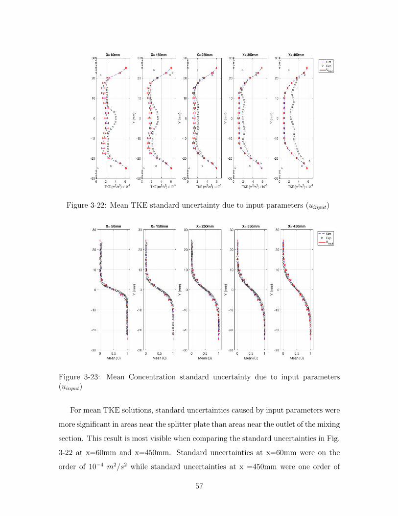
Figure 3-22: Mean TKE standard uncertainty due to input parameters (uinput)
Figure 3-23: Mean Concentration standard uncertainty due to input parameters(uinput)
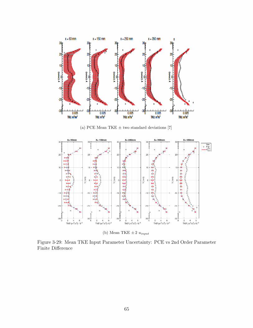
For mean TKE solutions, standard uncertainties caused by input parameters were
more significant in areas near the splitter plate than areas near the outlet of the mixing
section. This result is most visible when comparing the standard uncertainties in Fig.
3-22 at x=60mm and x=450mm. Standard uncertainties at x=60mm were on the
order of 10−4 m2/s2 while standard uncertainties at x =450mm were one order of
57
Page 58
Figure 3-24: Mean Velocity standard uncertainty due to input parameters (uinput)
magnitude less at 10−5 m2/s2. The standard uncertainties near the splitter plate
are a direct result of uncertainties caused by the inlet turbulent intensity conditions.
The higher the turbulent intensity at the inlet, the greater the TKE near the splitter
plate. Previous results in Fig. 3-22 support this result, demonstrating that the TKE
profile solution is most directly affected by the turbulent intensity at the inlet near
the splitter plate. That is, the highest sensitivity index occurs at x=60mm. However,
as the flow develops downstream the mixing section, the sensitivity of the TKE profile
solution to the turbulent intensity conditions decreases. This sensitivity coefficient
pattern is consistent with the smaller input parameter uncertainties demonstrated in
Fig. 3-22 near the outlet.
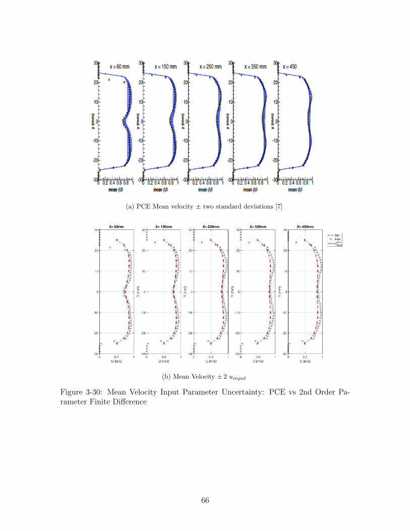
Standard uncertainties produced by input parameters are less significant for mean
x-component velocity profiles and mean concentration profiles. The effects of turbu-
lent intensity tends to not affect the mean x-component velocity profile along the
mixing section. The input standard uncertainty for the mean x-component velocity
profile was on the order of 10−3 m/s all throughout the mixing section. Standard
uncertainties due to input parameters were larger near the splitter plate for concen-
tration profiles, but not by an order of magnitude as was seen in the TKE profile
58
Page 59
shapes. Input parameter uncertainties for the concentration profiles were low near
the walls, and on the order of 10−2 in the mixing layer.
3.3 Uncertainty Quantification Methodology Re-
sults Comparison
In this section the results presented in the PCE study — conducted by Politecnio Di
Milano (PDM) researchers [7] — will be compared to the results presented in section
3.2.3 above.
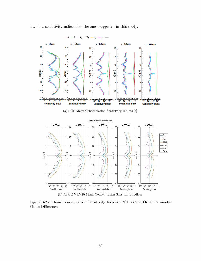
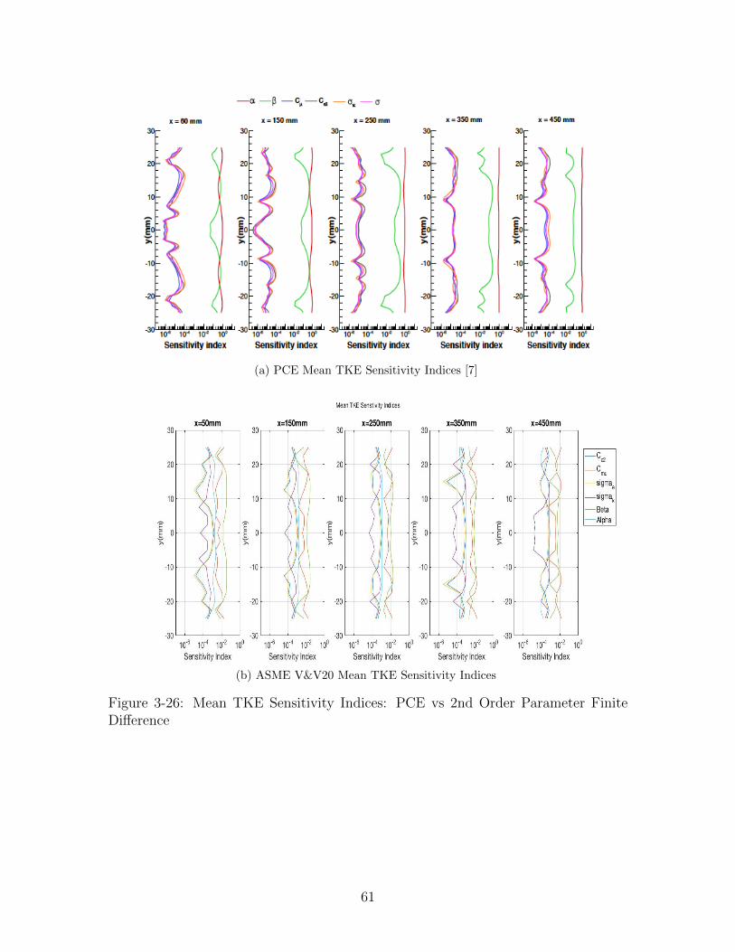
The profile shape of the sensitivity indices produced by the PCE and the ASME
V&V20 method demonstrate noticeable differences, however, the two methods share
similar conclusions. Taking a look at Fig. 3-25, 3-26, and 3-27 it is shown that the
smallest sensitivity indices for both methods are contributed by k-e turbulence model
coefficients (σε , σκ , Cε2). For the PCE study, Cµ has a much smaller contribution to
the overall solution sensitivity than what is reported in this study using the ASME
V&V20 methodology. As mentioned previously, the large sensitivity indices presented
for Cmu in this study can be contributed to the large influence of small standard
deviations on the parameter finite difference equation (Eq. 2.30). Another conclusion
is that both methods show that overall GEMIX model solution is most sensitive to
the turbulent intensity (β) conditions at the inlets. In addition, the β sensitivity
profile shape is closely mirrored between the two methods for mean TKE and mean
velocity.
The biggest discrepancy in the results is in the influence of the random velocity
profile variable α. In the PCE study it was found that the shape of the velocity profile
had the largest effect on the overall GEMIX simulation solution. Using the method
described in the ASME V&V20, it was found that α had a marginally smaller effect
on the GEMIX simulation solution than β. A deeper analysis of the velocity profile
along the inlet legs is necessary, for it is possible that the velocity profile is being
developed along the inlet lets. If this is the case, then velocity profile is expected to
59
Page 60
have low sensitivity indices like the ones suggested in this study.
(a) PCE Mean Concentration Sensitivity Indices [7]
(b) ASME V&V20 Mean Concentration Sensitivity Indices
Figure 3-25: Mean Concentration Sensitivity Indices: PCE vs 2nd Order ParameterFinite Difference
60
Page 61
(a) PCE Mean TKE Sensitivity Indices [7]
(b) ASME V&V20 Mean TKE Sensitivity Indices
Figure 3-26: Mean TKE Sensitivity Indices: PCE vs 2nd Order Parameter FiniteDifference
61
Page 62
(a) PCE Mean Velocity Sensitivity Indices [7]
(b) ASME V&V20 Mean Velocity Sensitivity Indices
Figure 3-27: Mean Velocity Sensitivity Indices: PCE vs 2nd Order Parameter FiniteDifference
62
Page 63
PCE and ASME V&V20 results are compared with experimental measurements in
Fig. 3-28, 3-29, and 3-30. The PCE mean with ± two standard deviations as well as
the experimental results are plotted on top (plot a). The simulation results obtained
in section 3.2.1 with ± two standard deviations of input parameter uncertainty —
U95%input = 2 ∗ uinput — and experimental results are plotted on the bottom (plot b).
An analysis of these plots show that the ASME V&V20 method produces smaller
input uncertainty boundaries than the PCE methodology (with mean concentration
being the exception). In Fig. 3-29, PCE mean TKE uncertainty bounds tend to be
larger than the uncertainty bounds produced using the ASME V&V20 methodology.
Similarly, in Fig. 3-30, the uncertainty bounds for the velocity profile in the bottom
chart (ASME V&V20) are much lower in magnitude in contrast to the uncertainty
bounds in the top chart (PCE). A potential explanation for the larger PCE uncer-
tainty bounds is the greater sensitivity of the PCE TKE and velocity solutions to the
random velocity profile variable α.
It should be noted that for mean concentration values uncertainty bounds are low
in magnitude for both UQ methods; indicating that uncertainties caused by input
parameters do not effect the concentration significantly. In general, experimental
concentration measurements tended to fall within the input parameter uncertainty
bounds for both UQ methods. For TKE and velocity profiles, however, only the
PCE method bounded experimental measurements in input parameter uncertainty
estimates. The ASME V&V20 input parameter uncertainty bounds produced for
the velocity profile were very small, indicating little sensitivity to input parameter
choice and not touching any experimental measurements. The ASME V&V20 input
parameter uncertainty bounds produced for the TKE profile were significantly more
pronounced; showing an influence to input parameter. The ASME V&V20 TKE
profile uncertainty bounds captured experimental TKE measurements near the edge
of the mixing layer, but failed in touching experimental measurements in the center
of the mixing section (y=0mm).
63
Page 64
(a) PCE Mean Concentration ± two standard deviations [7]
(b) Mean Concentration ± 2 uinput
Figure 3-28: Mean Concentration Input Parameter Uncertainty: PCE vs 2nd OrderParameter Finite Difference
64
Page 65
(a) PCE Mean TKE ± two standard deviations [7]
(b) Mean TKE ± 2 uinput
Figure 3-29: Mean TKE Input Parameter Uncertainty: PCE vs 2nd Order ParameterFinite Difference
65
Page 66
(a) PCE Mean velocity ± two standard deviations [7]
(b) Mean Velocity ± 2 uinput
Figure 3-30: Mean Velocity Input Parameter Uncertainty: PCE vs 2nd Order Pa-rameter Finite Difference
66
Page 67
3.4 Limitations and Potential Sources of Error
One of the main challenges experienced when performing the ASME V&V20 method
was quantifying the discretization error. In particular, the size of the modeled domain
and the relatively small variation of the distribution in the geometry make it particu-
larly challenging to adopt a sufficiently large refinement ratio. The current standard
suggests coarsening the grid by a grid ratio 2. In this particular instance coarsening
the grid by a ratio of 2 would result grid that could not capture the physics occurring
near the mixing layer, which would in turn lead to high discretization errors. In order
to avoid not capturing the mixing layer physics three grids with a refinement ratio
of 1.4 was selected. Using a three grid discretization study lead to difficulties with
asymptotic convergence of solutions. Thus, producing localized numerical uncertain-
ties that underestimate or overestimate actual numerical uncertainties. Advancement
in a method applicable to turbulent simulations with finite volume second order meth-
ods would greatly be welcomed by the community. For example, least square GCI
provides a manner in which to deal with non-monotonic convergence, but requires
adoption of large conservative margins and therefore large final uncertainty.
One of the difficulties with performing an uncertainty quantification study is as-
sessing input parameters. Inserting improper input parameters into a uncertainty
quantification study will result in meaningless results. Thus, ensuring that bounds
placed on parameters are correct is essential in a proper UQ study. In this study, the
velocity profile shape was described by a random variable α with a uniform proba-
bility distribution. The validity of this assumption is not known, hence using this
assumption may lead to an overestimation or underestimation of input parameter
uncertainty.
It is important to also note that results compared between the PCE study and this
study came from different CFD codes. The simulation used in this ASME V&V20
study was produced using STAR-CCM+ software. The simulation used to in the
PCE study was ANSYS FLUENT CFD software. In order to best compare the
results from these two CFD codes an intentional effort was made to keep physical
67
Page 68
models, boundary conditions, and initial conditions as consistent as possible.
The lack of experimental uncertainty results currently means that a full validation
cannot be conducted on the GEMIX simulation. Additionally, a need exists for more
accurate TKE profile results near the pressure outlet of the GEMIX. Currently, the
TKE profile at x=450mm contains larger TKE values than some profiles closer to the
splitter plate.
68
Page 69
Chapter 4
Conclusion & Future Work
In this study the ASME V&V20 methodology was used to to quantify the uncer-
tainty of CFD simulations of the GEMIX experiment. Due to lack of experimental
uncertainty data, this study proceeded to verify the solution by computing the numer-
ical and input parameter uncertainties. The input parameter uncertainty evaluated
using the ASME V&V20 methodology was then compared to a Polynomial Chaos
Expansion method for quantifying input parameter uncertainty.
GEMIX simulation results matched fairly well with experimental and mean PCE
results previously presented. The under predicted TKE profile values at x=60mm
were attributed to the k-e model not capturing larger coherent eddy structures that
drive mixing near the splitter plate. Similarly, slight over predictions in mixing layer
thickness were contributed to the k-e model’s tendency to over predict eddy viscosity.
All TKE, velocity, and concentration plots along the mixing section were consistent
with physics associated to developing flow.
Discretization error was found to be most prominent near the splitter plate on
the center plane (y=0mm) than in other regions along the mixing section. Numerical
uncertainty for concentration profiles were found to be overly conservative and un-
physical, with some localized numerical uncertainties ranging between ±0.77. This
result was expected, since for a coarser mesh the mixing layer is less pronounced and
the eddy viscosity becomes averaged over a larger cell (artificially increasing the size of
the mixing layer.) The TKE profile shows a maximum numerical uncertainty bound
69
Page 70
of ±0.01 m2/s2 at y=± 5mm and x = 60mm. Discretization error for the TKE
profile near the center of the mixing section (i.e. y=0mm) was shown to decrease
downstream. The velocity profile was found to be most insensitive to discretization
error with the large numerical uncertainty being on the order of 102 m/s.
An investigation into the Richardson extrapolation method highlighted challenges
associated with asymptotic convergence of localized values. An investigation of TKE,
concentration, and velocity observed p values showed a great variance dependent on
y-axis location. Most of these localized values were in oscillatory convergence, with
very few in monotonic convergence. An issue that led to these instabilities was the
particular physics of the mixing layer case. When performing the grid coarsening the
refinement along the mixing layer was lost, causing sharp gradients near the mixing
layer.
In order to perform the input parameter uncertainty analysis, six stochastic vari-
ables were introduced to handle uncertain boundary conditions and the coefficients
in the k-e turbulence model. Using the distribution parameters described in Table
3.3, the sensitivity coefficients and input parameter uncertainties were solved for. The
sensitivity coefficient study concluded that the turbulent intensity inlet condition was
the most influential parameter in the computation of TKE, U, and concentration pro-
files. The sensitivity coefficients also showed that the influence of the k-e turbulence
model coefficients is small. Using the sensitivity coefficients the input parameter un-
certainties were solved for TKE, U and concentration. Input parameter uncertainties
for mean TKE profiles were found to be most significant near the splitter plate, while
input parameter uncertainties were found to be less significant for mean x-component
velocity and mean concentration profiles. Having independent parameters was shown
to be an important limitation using the sensitivity coefficient method suggested by
the ASME V&V20 standard.
Input parameter uncertainties and sensitivity coefficients from this study were
then compared with mean PCE uncertainties / sensitivity indices and experimental
measurements. Mean PCE uncertainty bounds were found to be larger than the un-
certainty bounds solved through the ASME V&V20 input uncertainty study. The
70
Page 71
larger uncertainty in the PCE could potentially be caused by the greater PCE solu-
tion dependence on the velocity profile parameter α. Most PCE uncertainty bounds
touched or captured experimental measurements, but the input parameter uncertain-
ties in this study only captured concentration measurements.
The work conducted in this study has shown that even benchmark turbulent mix-
ing cases experience difficulties when the ASME V&V20 methodology is applied for
uncertainty quantification. Limitations associated with the ASME V&V20 methodol-
ogy include the need for solution asymptotic convergence, loss of physics when coars-
ening grid in limited geometric space, the need for independent variables to compute
sensitivity coefficients, and the need for accurate parameter boundaries (General UQ
issue). This study did show, however, that despite these limitations, input parameter
uncertainty results were similar between the ASME V&V20 method and the PCE
method.
Future work in this area should focus on resolving the limitations and potential
sources of error described in section 3.4. A least squared Richardson extrapolation
should be conducted on the GEMIX simulation to get better asymptotic convergence
data. An investigation should be conducted on the GEMIX inlet profile to help reduce
the uncertainties associated with the random parameter α. A PCE analysis should
be conducted using the data from this study to reduce the uncertainties associated
with using different CFD codes.
71
Page 73
Bibliography
[1] U.s. nuclear power plants. ”https://www.nei.org/Knowledge-Center/Nuclear-
Statistics/US-Nuclear-Power-Plants”, 2016.
[2] U.s. energy information administration - eia - independent statistics and analysis.
”https://www.eia.gov/nuclear/”, 2014.
[3] KEITH RIDLER. Feds announce $82 million for nuclear energy research.
”http://bigstory.ap.org/article/74050bc0b3c546dfb7b6da512189a559/feds-
announce-82-million-nuclear-energy-research”, 06 2016.
[4] Neams: The nuclear energy advanced modeling and simulation program.
”https://energy.gov/sites/prod/files/2013/07/f2/NEAMS
[5] The consortium for advanced simulation of lwrs. Web, May 2017.
[6] Standard for Verification and Validation in Computational Fluid Dynamics and
Heat Transfer - V&V 20, 2009.
[7] Antonio Buccio. Uncertainty quantification of cfd simulation for turbulent mix-
ing. n.p., 2015.
[8] K-J. Metzner U Wilke. Thermal fatigue evaluation of piping system ”tee” —
connections (therfat). Nuclear Engineering and Design, 235:473–484, 2005.
[9] C Walker M Simiano R Zboray H-M Prasser. Investigations on mixing phe-
nomena in single-phase flows in a t-junction geometry. Nuclear Enginering and
Design, 2009.
73
Page 74
[10] S. Chapuliota C. Gourdina T. Payenb J.P. Magnaudc A. Monavond. Hydro-
thermal-mechanical analysis of thermal fatigue in a mixing tee. Nuclear Engi-
neering and Design, 2005.
[11] Elia Merzari Andres Alvarez Oana Marin Aleksandr Obabko Steve Lomper-
ski Shashi Aithal. Thermal striping in nuclear reactors: Pod analysis of les
simulations and experiment. APS Division of Fluid Dynamics, 2015.
[12] Hyeong Kweon Jong Kim Jang Lee. Fatigue design of nuclear class 1 piping
considering thermal stratification. Nuclear Engineering and Design, 2008.
[13] Paul Scherrer Institute. Facility projects. https://www.psi.ch/teg/projects, 04
2017.
[14] A Badillo B Niceno J Fokken R Kapulla. Uncertainty quantification of the effect
of random inputs on computational fluid dynamics simulations of the gemix
experiment using metamodels. 2014.
[15] J Fokken R Kapulla G Galgani O Schib K Pawa H.M. Prasser. Lif-measurements
and self-similarity considerations in a stably stratified isokinetic turbulent mixing
layer. 2010.
[16] E.C. Eggertson R Kapulla J Fokken H.M Prasser. Turbulent mixing and its
effects on thermal fatigue in nuclear reactors. International Journal of Mathe-
matical, Computational, Physical, Electrical and Computer Engineering, 2011.
[17] Ronald Adrian Jerry Westerweel. Particle Image Velocimetry. Cambridge Uni-
versity Press, 2011.
[18] M. Raffel C.E. Willert S.T. Wereley J. Kompenhans. Particle image velocimetry:
A practical guide. Springer Berlin Heidelberg, 2017.
[19] H.M. Prasser A. Bottger J. Zschau. A new electrode-mesh tomograph for gas-
liquid flows. Flow Measurement and Instrumentation, 1998.
[20] LaVision. Lif in liquid fluids, product manual.
74
Page 75
[21] LaVision. Focus on fluid dynamics. Web., 2017.
[22] Laser induced fluorescence. http://www.lavision.de/en/techniques/lif-
plif/index.php, 04 2017.
[23] F.H. Harlow and J.E. Fromm. Computer experiments in fluid dynamics. Scien-
tific Journals, 212(3):104–110, 1965.
[24] F. G. Blottner. Introduction to the proceedings of the 3rd aiaa computational
fluid dynamics conference. In Proceedings of the 3rd AIAA Computational Fluid
Dynamics Conference, pages 1–2, June 1977.
[25] P.J. Roache, K. Ghia, and F. White. Editorial policy statement on the control
of numerical accuracy. ASME Journal of FLuids Engineering, 108(1):2, 3 1986.
[26] European research community on flow, turbulence,
and combustion best practices guidlines for cfd.
http://www.ercoftac.org/publications/ercoftac best practice guidelines/dispersed multi-
phase flows dmpf/.
[27] Charles Hirsch. A thematic network for quality and trust in the industrial ap-
plication of computational fluid dynamics (qnet-cfd). Chinese Journal of Aero-
nautics, 19:105–113, 05 2006.
[28] Best practice guidelines for the use of cfd in nuclear reactor safety applications.
OECD Nuclear Energy Agency, 2015.
[29] International vocabulary of basic and general terms in metrology. In Interna-
tional Organization for Standardization, 2nd, Geneva,Switzerland, 1993.
[30] H.W. Coleman W.G. Steele. Experimentation and Validation, and Uncertainty
Analysis for Engineers. John Wiley & Sons, 3rd edition, 2009.
[31] H.W. Coleman F. Stern. Uncertainties in cfd code validation. ASME J. Fluids
Engineering, 119:795–803, 12 1997.
75
Page 76
[32] L. F. Richardson. The approximate arithmetical solution by finite differences
of physical problems involving differential equations, with an application to the
stresses in a masonry dam. Transactions of the Royal Society of London, 1910.
[33] L.F. Richardson A.J. Gaunt. The deferred approach to the limit. part i. single
lattice. part ii. interpenetrating lattices. Transactions of the Royal Society of
London, 1927.
[34] Patrick J. Roache. Verification And Validation In Computational Science And
Engineering. Hermosa Publishers, 1998.
[35] L. Eca M. Hoekstra. An evaluation of verification procedures for cfd applications.
24th Symposium on Naval Hydrodynamics, 07 2002.
[36] J.H. Ferziger. Estimation and reduction of numerical error. In ASME Winter
Annual Meeting, San Fransisco, CA, 12 1989.
[37] P.J. Roache K. Ghia I.B. Celik C.J. Freitas H.W. Coleman P.E. Raad. Pro-
cedure for estimation and reporting of uncertainty due to discretization in cfd
applications. ASME Journal of Fluids Engineering, 130(7):4, 07 2008.
[38] Test uncertainty. ASME PTC 19.1-2005, 2005.
[39] Iso guide to the expression of uncertainty in measurement. ISO, 1995.
[40] Arnoldo Badillo Bojan Niceno. Uncertainty quantification in cfd simulations of
isokinetic turbulent mixing layers. In The 15th International Topical Meeting on
Nuclear Reactor Thermal-Hydraulics, 2013.
[41] Matthew Dunn Babak Shotorban Abdelkader Frendi. Uncertainty quantification
of turbulence model coefficients via latin hypercube sampling method. Journal
of Fluids Engineering, 2011.
[42] Stephen Pope. Turbulent flows. Cambridge university press, 2000.
76