Assessing the Real-Time Informational Content

of Macroeconomic Data Releases for Now-/Forecasting GDP:

Evidence for Switzerland§

Boriss Siliverstovs∗ Konstantin A. Kholodilin∗∗

December 5, 2009

Abstract

This study utilizes the dynamic factor model of Giannone et al. (2008) in order to make now-/forecasts

of GDP quarter-on-quarter growth rates in Switzerland. It also assesses the informational content of

macroeconomic data releases for forecasting of the Swiss GDP. We find that the factor model offers

a substantial improvement in forecast accuracy of GDP growth rates compared to a benchmark naive

constant-growth model at all forecast horizons and at all data vintages. The largest forecast accuracy is

achieved when GDP nowcasts for an actual quarter are made about three months ahead of the official

data release. We also document that both business tendency surveys as well as stock market indices

possess the largest informational content for GDP forecasting although their ranking depends on the

underlying transformation of monthly indicators from which the common factors are extracted.

Keywords: Business tendency surveys, Forecasting, Nowcasting, Real-time data, Dynamic factor model

JEL code: C53, E37.

§We are grateful to Domenico Giannone for sharing with us the code used in Giannone et al. (2008). We also acknowledgethe help related to data access and management we received from Christian Busch, Matthias Bannert as well Fabiano Cuccu.All the computations have been performed in OX version 5.10 (Doornik, 2007), figures—in R-2.9.2.

∗ETH Zurich, KOF Swiss Economic Institute, Weinbergstrasse 35, 8092 Zurich, Switzerland, e-mail:

boriss.siliverstovs@kof.ethz.ch∗∗DIW Berlin, Mohrenstraße 58, 10117 Berlin, Germany, e-mail: kkholodilin@diw.de

1 Introduction

This paper explores the real-time informational content of various macroeconomic data releases both for

nowcasting and one-quarter-ahead forecasting of the Swiss GDP employing the approach suggested in Gian-

none et al. (2008). Giannone et al. (2008) provide a unified statistical framework that combines the following

aspects characterizing the real-life decision-making process of a policy maker: i) extraction of a (useful) sig-

nal from a large number of various economic indicators, ii) accounting for asynchronous releases of various

blocks of macroeconomic data when updating actual now-/forecasts such that a typical situation of being

confronted with an unbalanced panel of available indicators—a so called ”jagged edge”—is naturally incor-

porated into the statistical model, iii) ”bridging” the economic indicators available at the monthly frequency

with the quarterly GDP now-/forecasts.

Giannone et al. (2008) suggest using an approximate dynamic factor model estimated in two steps. In the

first step the common factors are extracted by the static principal components analysis using the balanced

panel of monthly indicators. The balanced panel is achieved by truncation of the available unbalanced panel

at the data block with the largest publication lag. In the second step the common factors are extracted by

means of Kalman filter for the whole sample of interest.

By now, the use of a large-scale factor models for economic forecasting enjoy a wide popularity (e.g.,

see Siliverstovs and Kholodilin, 2009; Schumacher and Breitung, 2008; Schumacher, 2007; Kholodilin and

Siliverstovs, 2006; Forni et al., 2005; Stock and Watson, 2002a,b; Sancho and Camacho, 2002; Artis et al.,

2001; Forni et al., 2000, inter alia). The approach of Giannone et al. (2008) distinguishes itself from this

extensive literature in that it is the first study attempting to single out marginal change in forecast accuracy

attributable to a particular block release of macroeconomic data. According to Giannone et al. (2008), a

block release that effects the forecast accuracy to the largest extent possesses also the most of real-time

information helping predicting quarterly GDP.

Our study contributes to the literature in the following three ways. First, to the best of our knowledge,

it represents the first attempt to predict the growth rate of the Swiss GDP for the current quarter (nowcast)

as well as for the next quarter (forecast) using a large-scale factor model. The previous research either used

a single leading indicator model (Muller and Koberl, 2008) or it used a leading indicator (KOF-Barometer)

extracted from a small-scale static factor model (Graff, 2009; Siliverstovs, 2009) for predicting GDP growth

rates in Switzerland. Our study also distinguishes itself from these studies in that we choose the quarter-on-

quarter seasonally adjusted GDP growth rates as a target prediction variable rather than the year-on-year

quarterly GDP growth rate that these earlier studies aimed to predict. In doing so, we conform to Giannone

et al. (2008) in the choice of the variable of interest.

Second, despite a wide applicability of factor-based models, the research question on the informational

content of different macroeconomic data releases pursued in Giannone et al. (2008) so far did not gain much

popularity. In fact, we are aware of only one additional study that investigates this issue; Aastveit and

Trovik (2007) provide another case study for Norway. It is worthwhile noting that these both studies arrive

at somewhat contradictory conclusions regarding which block of variables has a largest positive impact on

1

forecast accuracy. Giannone et al. (2008) conclude that the Philadelphia Federal Bank surveys as well as

the report on the employment situation contribute the most to increase in forecast accuracy whereas the

impact of financial variables (including several stock market indices) is found to be negligible. On contrary,

Aastveit and Trovik (2007) find that the stock market variables are an important factor in reducing forecast

uncertainty1. In a given situation our study provides another case study investigating importance of various

data releases for now-/forecasting GDP. In our study both stock market and the business tendency surveys

are included in the factor model allowing us to compare the contribution of these variables to forecast

accuracy reinforcing conclusions of either of these two studies.

Third, in our simulation of a real-time forecasting we attempt to perform as to the largest extent possible.

In particular, we utilize the real-time vintages of the target variable—the seasonally adjusted quarter-on-

quarter GDP growth rates—and access the contribution of various data releases to improvement of forecast

accuracy with respect to the first officially figure published by the State Secretariat for Economic Affairs

(SECO). The importance of using real-time instead of latest-available data has been already emphasized in

numerous studies as it has been shown, for example, by Diebold and Rudebusch (1991) and, more recently,

by Croushore (2005) that the favorable conclusions on forecasting properties of leading indicator indexes

obtained using latest-available data may be substantially weakened or even reversed when forecasting exercise

is replicated using real-time data sets. Furthermore, the real-time flavor is also kept as much as possible in

constructing the panel of our monthly indicators. Some of them undergo no (stock market variables, interest

rates and exchange rates) or rather minor revisions (business tendency surveys). At the same time we have

several blocks of the variables (trade and retail variables, prices, and employment) that were subject to both

seasonal adjustment and later revisions for which we have no real-time vintages.

We find that the factor model offers a substantial improvement in forecast accuracy of GDP growth rates

compared to a benchmark naive constant-growth model at all forecast horizons and all data vintages. The

largest forecast accuracy is achieved when GDP nowcasts for an actual quarter are made about three months

ahead of the official data release. We also document that both business tendency surveys as well as stock

market indices possess the largest informational content for GDP forecasting although their ranking depends

on the underlying transformation of monthly indicators from which the common factors are extracted.

The paper is structured as follows. In Section 2 the modeling approach of Giannone et al. (2008) is

presented. Section 3 contains description of data used. The results of our forecasting exercise are presented

in Section 4. In the next section the model performance in forecasting the current crisis is scrutinized. The

final section concludes.

2 Model

As mentioned above, an important feature of the approach of Giannone et al. (2008) is that it allows to

measure the marginal impact on reduction in model prediction uncertainty as new macroeconomic data are

released. In order to see this, we need the following notation. Denote Ωv a collection of all information sets

1Aastveit and Trovik (2007) does not include surveys in the their factor model as they are only available at the quarterlyfrequency in Norway.

2

that correspond to the flow of b blocks of newly released macroeconomic data during a month v, such that

Ωv = Ωvj ; j = 1, ..., b,

where

Ωvj = Xit|vj; t = 1, ..., Tivj ; i = 1, ..., n

is an information set available to a forecaster after a block j was released in a given month v. This information

set is comprised from monthly indicators Xit|vjwith the subindex i = 1, .., n indicating individual time series

and the subindex t = 1, ..., Tivj denotes the corresponding period of observed values for a given time series.

This means that Tivj denotes the last period for which time series i in vintage vj has a valid observation.

Furthermore, denote a quarter q by its last month. Then imposing the restriction that the sample starts

in the first month of a quarter, we have q = 3k with k = 1, 2, .... Due to a stable release pattern of monthly

data blocks a given vintage vj is released three times per quarter generating the following information sets

Ωvj with v = 3k − 2, 3k − 1, 3k in the first, second and third months of quarter, respectively.

Let y3k be GDP growth rate for a given quarter q = 3k. Then for each information set Ωvj with

v = 3k − 2, 3k − 1, 3k the forecast is computed as a projection of y3k on the available information set

y3k|vj= E

[y3k|Ωvj

;M], v = 3(k − h)− 2, 3(k − h)− 1, 3(k − h), j = 1, ..., b (1)

for a given underlying model M . The letter h denotes the forecast horizon such that for h = 1 we produce

one-quarter ahead forecasts and for h = 0 we produce forecasts for the current quarter, i.e., nowcasts.

Observe that Equation (1) denotes the so-called “bridge regression” that utilizes information available at

monthly frequency in order to forecast quarterly variable of interest.

Recall that the magnitude of interest is the uncertainty surrounding the forecast at a given vintage, or,

more precisely, its evolution over time from vintage to vintage. Following Giannone et al. (2008), we measure

the forecast uncertainty associated with a given vintage as follows

Vy3k|vj= E

[(y3k|vj − y3k)

2;M]. (2)

It is expected that as more timely data become available this uncertainty measure will have a tendency to

decrease, i.e., Vy3k|vj≤ Vy3k|vj−1

, allowing to assess informational content of each data block release.

Giannone et al. (2008) suggest a following approximate dynamic factor model with the monthly indicators

xt|vj = (x1t|vj, ..., xnt|vj

)′ are assumed to be driven by r unobserved common factors Ft = (f1t, ..., frt)′ with

r ≪ n and individual-specific idiosyncratic components ξt|vj = (ξ1t|vj, ..., ξnt|vj )

′ such that in matrix notation

the model reads

xt|vj= µ+ ΛFt + ξt|vj

, (3)

where µ = (µ1, ..., µn)′ is a vector of individual specific intercepts and Λ is a n× r matrix of factor loading

3

coefficients. The common factors are assumed to follow a vector autoregressive process

Ft = AFt−1 +But, ut ∼WN(0, Iq) (4)

where A is a r × r parameter matrix satisfying a stationarity restriction such that all roots of (Ir − Az) lie

outside the unit circle, B is a r × q matrix of full rank q, and ut is a q−dimensional white-noise process,

representing shocks to the common factors. Specifying the equation for factor dynamics allows one to imple-

ment the Kalman smoother in order to compute recursively the expected value of the common factors also

in the presence of missing observations in the end of the sample, i.e, the “jagged edge”, due to asynchronous

data releases.

Additional assumptions include a white-noise process for idiosyncratic shocks ξt|vj in Equation (2), i.e.,

E(ξt|vjξ′t−s|vj

) with s > 0 for all j and v, zero cross-correlation, i.e., E(ξt|vjξ′t|vj ) = Ψt|vj = diag(ψ1t|vj , ..., ψnt|vj

),

as well as the assumption of Gaussian error terms.

Denote the expected value of the common factors for a given underlying model M as

Ft|vj = E(Ft|Ωvj ;M)

and the associated factor estimation uncertainty as

Vvj = E[(Ft − Ft|vj )(Ft − Ft|vj)′;M)].

Both these quantities of interest are available as a standard output of the Kalman filter.

Giannone et al. (2008) suggest to compute now-/forecasts GDP by projecting the quarterly GDP growth

growth rates on the estimated monthly factors that have been converted to quarterly frequency by keeping

only their values in the last month of quarter, F3k|vjwith k = 1, ..., ⌊Tyvj/3⌋ where Tyvj is the last month in

quarter for which GDP is available for a given vintage vj . Thus, rather than projecting GDP on the whole

information set available for some vintage vj as shown in Equation (1) that may be a rather formidable

task, Giannone et al. (2008) suggest projecting on a few common factors resulting in a parsimonious forecast

model

y3k|vj= γ0 + γ′F3k|vj , (5)

whose parameters can be easily estimated by OLS. The h−quarter ahead forecasts are made for each of the

following months in quarter v = 3(k− h)− 2, 3(k− h)− 1, 3(k− h). Naturally, for h = 0 the nowcasts of the

current quarter GDP is produced.

The associated forecast uncertainty is computed as

Vy3k|vj= γ′Vvj γ + V ar(e3k|vj ),

where e3k|vj = y3k|vj− y3k|vj are the estimated residuals in the forecasting model.

4

3 Data

The data set of monthly indicators consists of 562 indicators sub-divided into the following 10 blocks: Pur-

chasing Managers Index in manufacturing supplied by Credit Suisse (9 time series, “PMGR”), consumer price

indexes (30, “CPI”), labour market indicators (6, “LABOUR”), producer price indexes (11, “PPI”), busi-

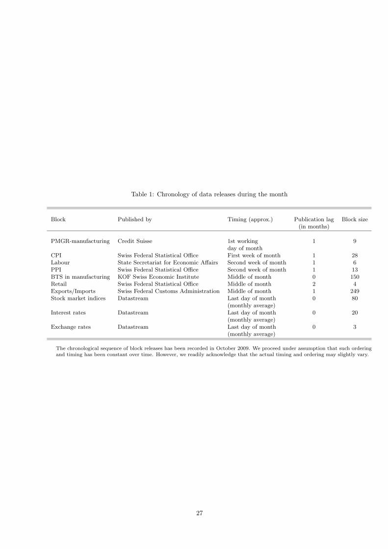
ness tendency surveys in manufacturing collected at the KOF Swiss Economic Institute (150, “CHINOGA”),

retail trade (4, “RETAIL”), exports and imports (249, “TRADE”), stock market indices (80, “STMKT”),

interest rates (20, “INT.RATE”), and exchange rates (3, “EXCH.RATE”). The chronological sequence of

block releases has been recorded in October 2009 and the further assumption has been made that it was

preserved during the forecast sample in our “pseudo” real-time exercise. It generally corresponds to the

actual release pattern although its timing and ordering may slightly vary from month to month in real life.

For each month we constructed 10 vintages of data reflecting gradual expansion of the available information

set by the newly released data.

Information on the monthly indicators is presented in Table 1. Observe that blocks of macroeconomic

data differ both in terms of size and timeliness. The largest block is the block containing the exports and

imports statistics, followed by the KOF surveys. The smallest block is one with the exchange rates, followed

by retail trade, labour-market indicators, and the PMGR block where the number of indicators is below 10.

In our setup the timeliest block is the KOF surveys released in the middle of the month with zero publishing

lag. Following Giannone et al. (2008), we consider only monthly averages of the financial variables that are

incorporated in the model at the end of each month. Observe that these variables are available at the daily

frequency and by considering their monthly averages we are likely to downplay importance of these variables

for forecasting accuracy, on the one hand. On the other hand, the informational content of the financial

variables, e.g., stock market indices, may be impaired by their high variability when those are followed at

daily frequency. In this case, considering only monthly averages is likely to smooth the noise out, thus

positively influencing forecast accuracy. The retail variables are those with the largest publication lag of two

months. The rest of blocks are released with lag of one month.

Prior to estimation all data except both blocks of surveys have been transformed to stationarity2. Fur-

thermore, Giannone et al. (2008) suggest to transform all variables in order to ensure that these correspond to

a quarterly quantity when observed at the end of the quarter3. In sequel we will refer to such transformation

as the end-of-quarter equivalent transformation (EQE-transformation, in short). For the sake of brevity, we

present both sets of the results, i.e., those based on original stationary variables and their quarterly-quantity

equivalents. The data set of monthly indicators that is balanced at the beginning of the estimation sample

after all necessary transformations and which is used for extraction of common factors starts in the first

month of last quarter of 2000, i.e., in 2000M10. A rather late starting date is mainly due to the fact that

the KOF business tendency surveys in manufacturing (“CHINOGA”-block) are only available since 1999.

The target variable that we forecast are the quarter-on-quarter seasonally adjusted GDP growth rates.

2See Appendix for the complete list of the monthly components and their transformation description.3This is achieved by application of the following filter on the initial monthly time series xt: yt = xt + 2 ∗ xt−1 + 3 ∗ xt−2 +

2 ∗ xt−3 + xt−4.

5

Since in real time a lot of attention is paid to the first officially released figures we assess the forecast accuracy

of our factor model with respect to that figure. To this end, we utilize the real-time vintages of all releases

of the target variable since the first quarter of 2005. The forecast sample ends in the second quarter of 2009,

leaving us with 18 forecasts per vintage.

4 Results

In this section we describe the obtained results. We do it for two sets of indicator variables. First, we consider

the data set composed using the variables transformed to stationarity (whenever necessary). In particular,

we apply the stationarity transformation to all blocks of variables except “CHINOGA”- and “PMGR”-

blocks. We spared these two blocks from stationarity transformation for following reasons: the application

of first-differencing of survey indicators resulted in much worse forecasting performance of the factor model

compared to the case without this transformation, and since these type of variables by construction are

bounded—a feature which is not consistent with properties of unit-root processes. Secondly, we follow

the suggestion of Giannone et al. (2008) and report the results obtained using the data set composed of

the transformed-to-stationarity variables for which their quarterly equivalents observed at the end of each

quarter were computed. For each data set we report the results obtained using the dynamic factor model

based on one extracted factor and then we check the robustness of these results by reporting those obtained

by extracting two factors.

We limit ourselves to the maximum of two extracted factors for the following reasons. First, the estimation

sample is rather limited leaving us with 15 observations used for estimation of parameters of the bridging

equation (5) in the very beginning of our forecasting exercise4. In the end, we have 34 observations for

producing the nowcast using the latest available information set—in the last month of the last reference

quarter 2009Q2. Hence by keeping the maximum number of factors to two we work with a parsimonious

forecasting model and are not exposed to the risk of overfitting the model. Secondly, both Giannone et al.

(2008) and Aastveit and Trovik (2007) use models with two common factors. Koop and Potter (2004) also

emphasize the importance of parsimony in model selection for forecasting reporting that an optimal number

of factors on average is close to two.

4.1 Data set with stationary indicators: without EQE-transformation

4.1.1 A factor model with q = 1, p = 1

We start the analysis of the forecasting performance of the dynamic factor model with its simplest speci-

fication; we allow for one common factor, i.e., p = 1, and, correspondingly, one common shock q = 1, see

Equations (3) and (4) describing the model.

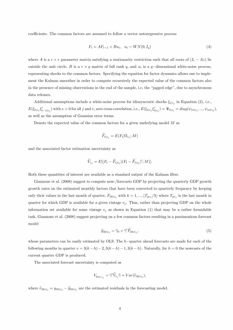
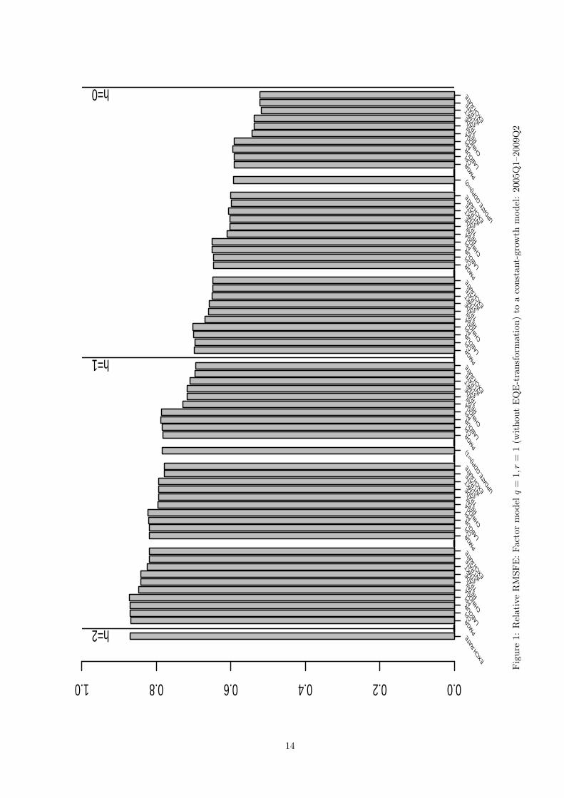
Figure 1 reports the relative RMSFE measure of the RMSFE obtained at a given vintage to the RMSFE

4The estimation sample of the bridge equation covers 2000Q4–2004Q2 in order to make the first h = 2 forecast of growthrate in 2005Q1 made in the last month of 2004Q3.

6

of a naive constant-growth model, estimated using the same period5. Each vintage within a given month

is labeled by the name of the corresponding block that expands the available information set. Observe

that in addition to ten vintages in each month we evaluate also the extent to which changes in forecasting

accuracy can be attributed to extending by one quarter the estimation sample used in the forecasting “bridge

regression” by incorporating the latest vintage of the quarterly GDP growth rates. We label such vintages

as “UPDATE.GDP (h=1)” and “UPDATE.GDP (h=0)” depending on the timing of the GDP update. In

this way we verify whether the estimated coefficients of the bridge regression change or not as a result of

increasing the estimation sample and of revisions in quarterly growth rates. In case of coefficient instability

we would observe large changes in the corresponding values of the RMSFE compared to that observed for

the previous data vintage based on the same set of monthly indicators. As shown below the estimated

coefficients in the bridge regression practically are not effected by such action.

In order to establish a benchmark for evaluating marginal changes in forecast uncertainty we started

with two-quarter ahead forecasts, h = 2, computed when all data releases for the respective quarter where

published. The corresponding relative RMSFE is the first bar on the left side of Figure 1. The next bar

“PMGR” corresponds to the model where the factor has been extracted from the data set updated in the

beginning of the first month in quarter by incorporating newly released Purchasing Managers’ Index block

that typically takes place in the first working day of month, see Table 1. Starting with the bar “PMGR” the

relative RMSFE are reported corresponding to one-quarter ahead forecasts produced during the next three

months. After these three months the bars correspond to the RMSFE for the models evaluated during the

forecast quarter, i.e., nowcasts.

Observe that the relative RMSFE is always less than one implying that our factor model offers an

improvement in forecast accuracy over the constant-growth model as far as two quarters ahead. Furthermore,

the relative RMSFE have a strong tendency to decrease as more and more information is utilized in making

out-of-sample forecasts. In fact, it decreases from 87% for the only two-quarter ahead forecast to 70% for the

best one-quarter ahead forecast, and then further to 52% for the best nowcast made in the last month of the

reference quarter. According to Figure 1 the biggest marginal decrease in the relative RMSFE occurs when

the business tendency surveys “CHINOGA” are incorporated into the model. According to Table 1, these

surveys are the first block with zero publication lag, i.e., it is related to the actual month when forecasts

being made. All data blocks released prior to “CHINOGA”-block have the publication lag of one month.

So far our results indicate that the largest informational content for forecasting have the business tendency

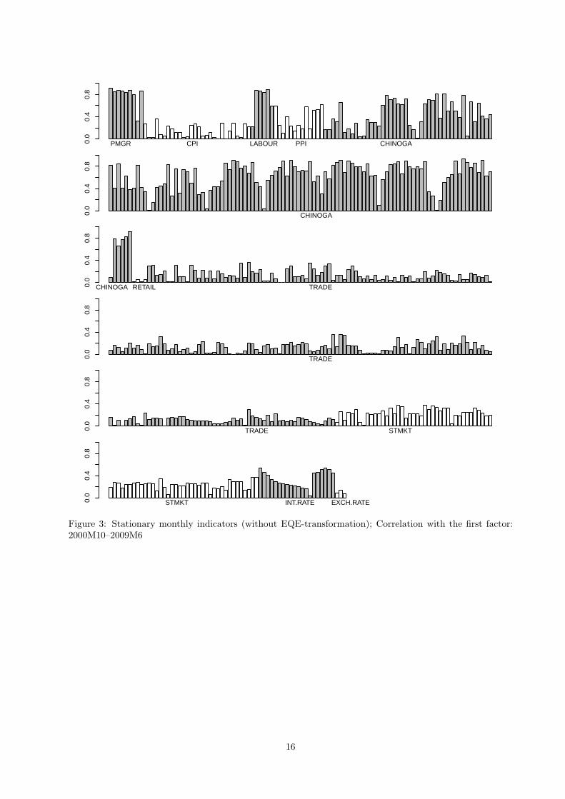
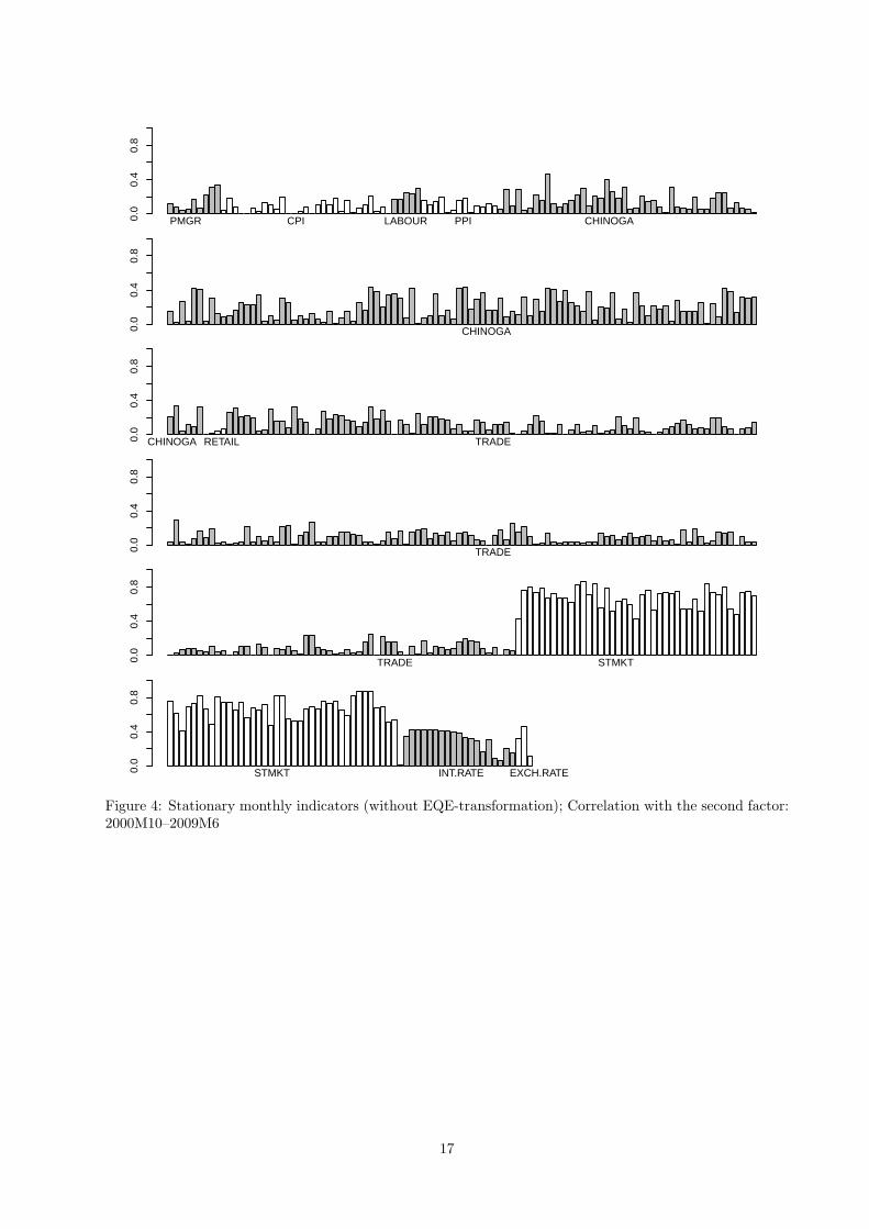
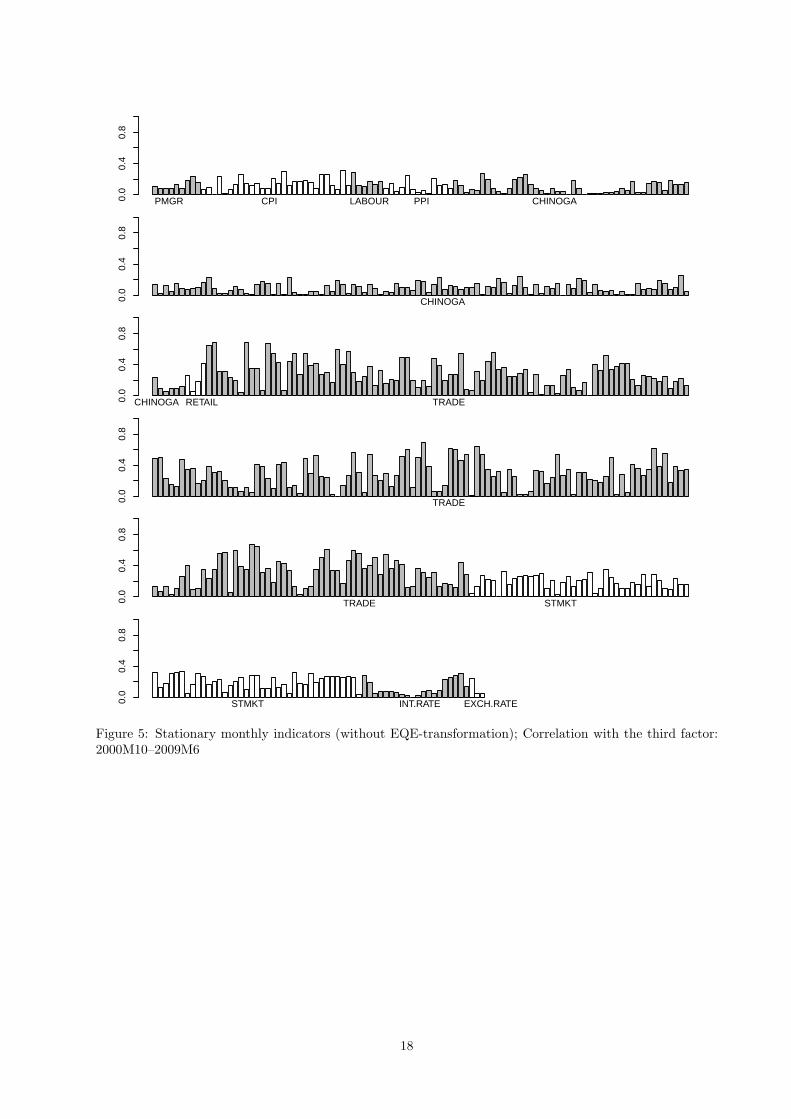
surveys collected at KOF. In order to understand driving forces behind this finding we plotted the (absolute)

correlations of extracted factors with the indicators, see Figures 3–5 for correlations with the first, the second,

and the third factors, respectively. As seen, there is a strong association of each factor with a particular

block(s) of variables. Thus, the first factor exhibits very high correlation with “PMGR”, “LABOUR”, and,

especially, with “CHINOGA”, which is the largest block among these three blocks. There also a medium-

strength correlation is observed with the block of interest rates. The second common factor primarily

5Using the extended sample starting in 1992Q1 for out-of-sample growth forecasts for a constant-growth model results inpractically the same results. Here we use the same estimation sample in order to make the RMSFE obtained by the competingmodels comparable.

7

correlates with the stock market indices “STMKT”. Finally, the third factor mostly correlates with the

exports-imports indicators although correlation strength is not that large.

Based on the correlation analysis we can readily explain the finding that the block “CHINOGA” has

the largest informational content in a given setup. First, this block of the variables exhibits the highest

correlation with the first common factor used to produce forecasts. Second, this block is the timeliest one,

i.e., in our chronological release sequence it is the first block containing information on the same month when

it is released. Hence the fact that newly released information that primarily feeds into the first common

factor and in doing so it clearly improves forecast accuracy seems to confirm aspirations of many economists

and policy-makers that the qualitative soft data in the form of business tendency surveys provide a useful

information on the current as well as future stand of economic activity in a timely manner. This finding also

conforms to that reached in Giannone et al. (2008) regarding the importance of surveys for nowcasting the

US economy.

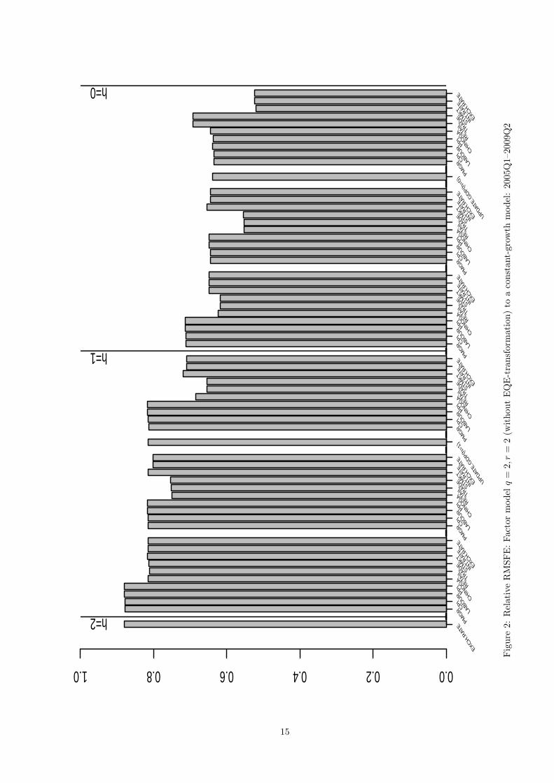
4.1.2 A factor model with q = 2, r = 2

In this subsection we investigate the robustness of the obtained results by evaluating forecasting performance

of the dynamic factor model with two common factors. Based on the results of the correlation analysis

presented above we impose two common factors p = 2 and two common shocks q = 2 that feed into these

common factors. Recall that the first common factor is primarily associated with “PMGR”, “LABOUR”,

and “CHINOGA” data blocks, whereas the second factor—with the block of stock market indices “STMKT”.

The resulting relative RMSFE are displayed in Figure 2. Several observations can be made. First, adding

the second factor to the forecasting model does not change the earlier result on the relatively large importance

of surveys. In fact the associated marginal increase in forecast accuracy is much stronger pronounced for

all “CHINOGA”-releases within a month except for the release in the last month of nowcasting quarter

when no noticeable improvement can be observed. Second, the incorporation of the block of stock market

indices “STMKT”, whose components are highly correlated with the second factor, somewhat obscures

forecast accuracy in this two-factor model. A likely reason for this surprising finding is that when extracting

common factors from the monthly data set we do not perform the transformation suggested in Giannone

et al. (2008) that converts monthly time series to its end-of-quarter equivalents. The sensitivity of the results

with respect to application of this transformation is investigated in the next subsection.

4.2 Data set with stationary indicators: EQE-transformation

4.2.1 A factor model with q = 1, r = 1

In this section we repeat the forecasting exercise but this time using monthly indicators converted to its end-

of-quarter equivalents as advocated in Giannone et al. (2008). Observe that this transformation is applied

to all blocks of variables but the “CHINOGA”-block where this transformation appears to superfluous and

unnecessary as it only results in much worse forecast performance. As the “PMGR”-block also represents

the business tendency surveys we likewise retained untransformed indicators in this block. Although the

8

question of whether to transform or not to transform the “PMGR”-block is of much less importance due to

the fact that it is released after the “CHINOGA”-block and its size is much smaller.

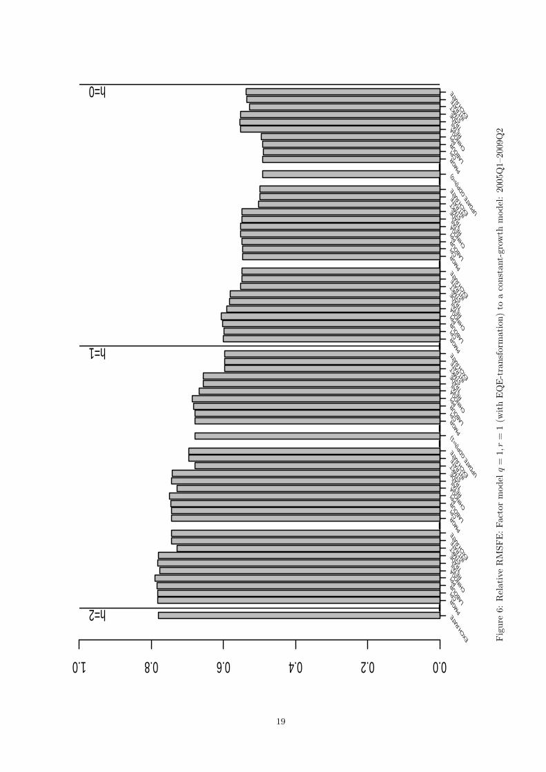
We start with the forecasting model based on one common factor. The corresponding relative RMSFE is

displayed in Figure 6. The first observation is that our earlier conclusion on the largest informational content

of surveys is no longer supported in this model. In fact, the largest marginal change occurs when the stock

market indices are incorporated in the forecasting model. This is true for all months except the last one

when inclusion of further data blocks starting with survey-block slightly worsens accuracy of nowcast. The

second observation is that the overall forecast accuracy when compared with the one-factor model without

such transformation has been boosted. Thus for the two-quarter ahead forecast the relative RMSFE ratio

has gone down from 87% to 78%, for the best one-quarter ahead forecast—from 70% to 60%, and finally for

the best nowcast—from 52% to 49% with an additional notice that the RMSFE ratio of 49% is achieved in

the beginning of the last month of quarter for the model with transformed variables whereas the RMSFE

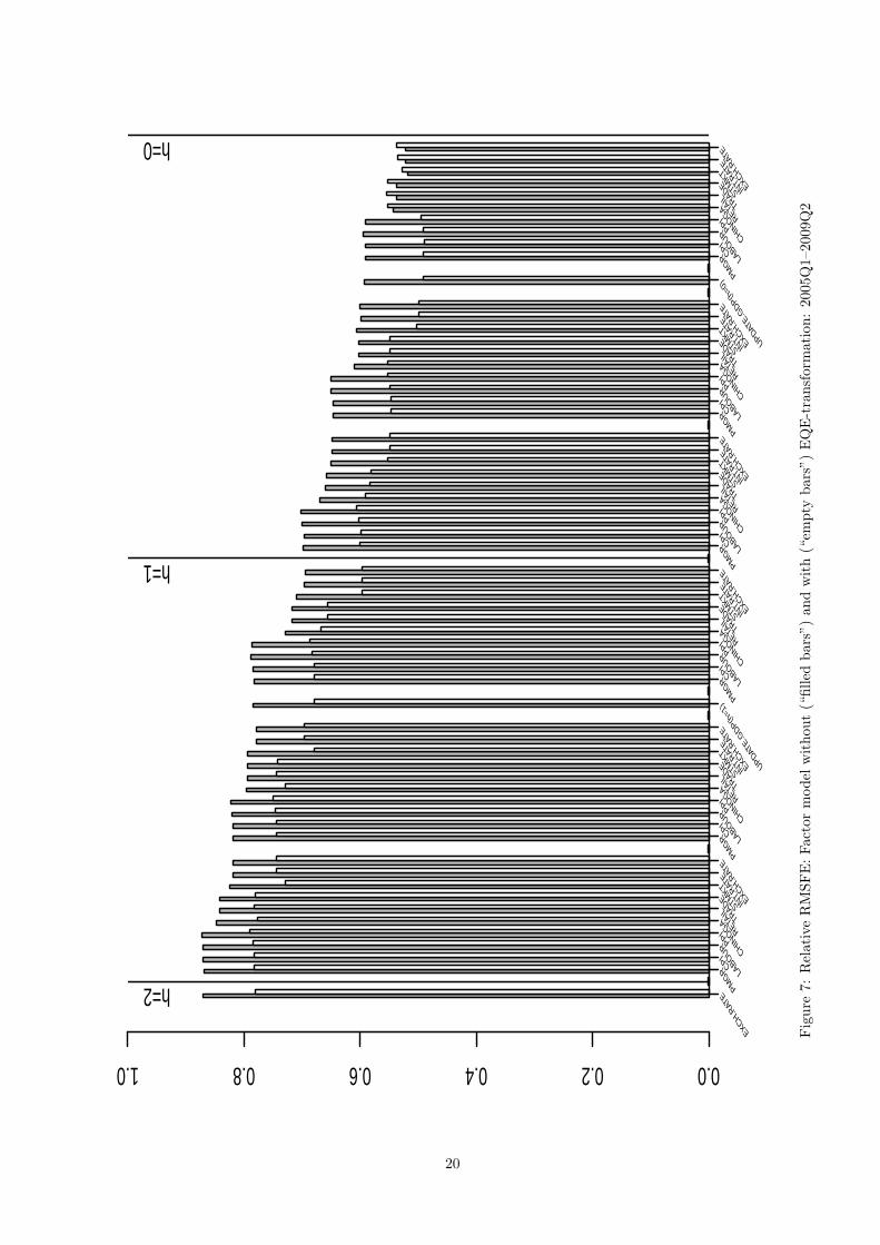
ratio of 52% is achieved in the end of the same month, i.e., at a much later point of time. Figure 7 compares

forecast performance of these two models confirming the superior forecast accuracy of the factor model based

on the transformed data.

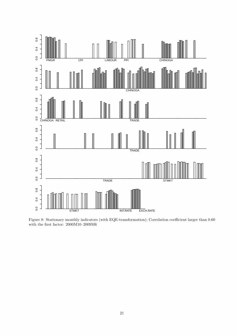
In order to understand the sources of improvement in forecast accuracy we compared correlations of the

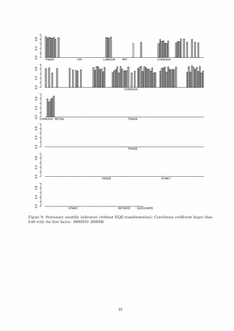
extracted factor with the transformed indicators, see Figure 8. The corresponding correlation with indicators

without EQE-transformation is presented in Figure 9. Observe that in order to facilitate comparison we

reported only correlations that in absolute value are larger than the chosen threshold of 0.60 in both figures.

The first thing to notice immediately that the first factor in the former model is highly correlated with

indicators from all blocks but “RETAIL” and “EXCH.RATE”. This is in sharp contrast to the earlier

finding that the first factor mostly correlates with “PMGR”, “LABOUR”, and “CHINOGA” blocks and the

selected correlations presented in Figure 9 further emphasize the point. Hence the former model exploits

information contained in different blocks composing the large panel to much better extent.

Analysis of correlations suggests also a tentative explanation why the earlier observation presented in

Section 4.1.1 on the largest informational content of “CHINOGA”-block is not supported in the current setup

but it is rather attributed to “STMKT”-block. According to Figure 8 both “CHINOGA”- and “STMKT”-

blocks appear to be the most important blocks that contribute to dynamics of the common factor. Hence

the release of “CHINOGA”-block earlier in the month represents only partial information that determines

the out-sample dynamics of the common factor, the remaining information is incorporated in the model only

when “STMKT”-block is released, jointly leading to improved forecast accuracy.

We also would like to make a comment regarding performance of the Purchasing Managers’ Index

(“PMGR”) block. According to both Figures 8 and 9 the variables in this block exhibit very high correlation

with the extracted factor. Hence it appears to be a highly relevant indicator that deservingly attracts a

lot of attention both by practitioners as well as by the media whenever it is released. In current setup we,

however, did not find that this block has a significant impact on forecast accuracy. This can be traced to

the fact that its release takes place more than two weeks later than the release of “CHINOGA”-block and

is barely preceded by incorporation of “STMKT”-block into the forecasting model. Hence the information

9

contained in “PMGR”-block is likely to be already accommodated in the forecasting model at the moment

of its release.

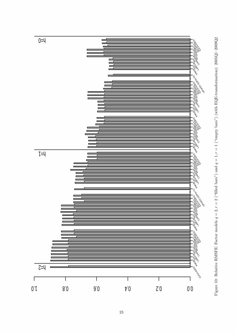
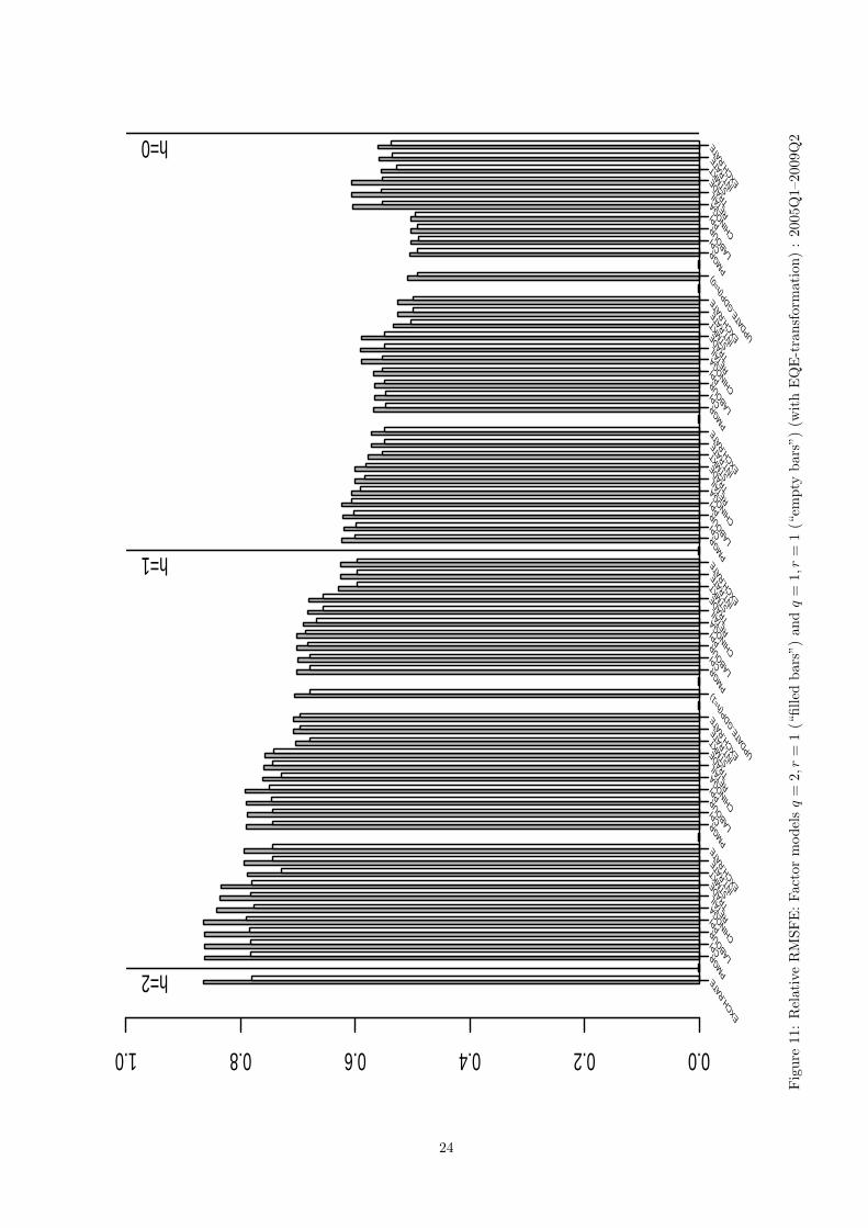
4.2.2 A factor model with q = 2, r = 2 and q = 1, r = 2

In this section we investigate the forecasting performance of factor models with two factors. More specifically,

first consider a model where we impose two common shocks q = 2 as well as two common factors r = 2,

similarly to the analysis reported in Section 4.1.2. Secondly, we consider an intermediate-case model with

one common shock feeding into two common factors, i.e., imposing q = 1, r = 2. The forecast performance

evaluation for the former and the latter models compared to that of the more parsimonious model with

q = 1, r = 1 considered in the previous section is presented in Figures 10 and 11, respectively. The main

conclusion drawn from these figures is that inclusion of the second factor into the forecasting model only

resulted in the inferior forecasting performance compared to a single-factor model. This implies that in a

given setup the common dynamics in our panel which is relevant to forecasting GDP is well captured by the

first common factor. This conclusion is also supported by the fact that in the forecasting “bridge regression”

the second factor was found to be insignificantly different from zero at the usual levels.

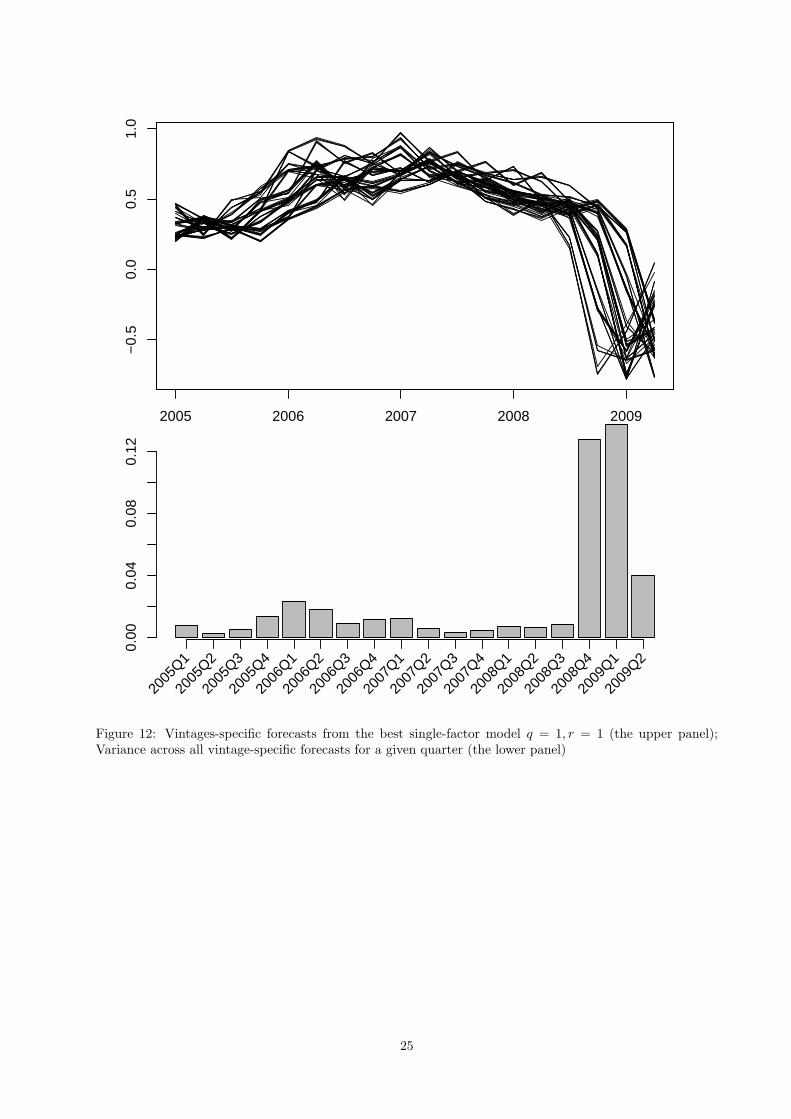
5 Forecasting GDP during the current crisis

In this section we further investigate how the factor model in its preferred specification performed during

the whole forecast sample paying a special attention to its ability to forecast the Swiss GDP during the

current crisis. The relevant information is displayed in Figure 12. The upper panel of Figure 12 displays all

vintage-specific forecasts, whereas the lower panel contains the variance of quarter-specific forecasts across all

vintages, measuring response sensitivity of subsequent forecasts to the continuous flow of new information.

It is striking to observe that during the pre-crisis period the computed dispersion has been largely constant

whereas since 2008Q4 we observe a sharp increase in forecast responsiveness to new pieces of information

illustrating the rapidly unfolding crisis triggered by the unexpected collapse of the Lehman Brothers in the

middle of September 2008. This can traced to the fact that the set of predictions for 2008Q4 consists both

of the forecasts made prior to the bankruptcy of the Lehman Brothers as well as of the nowcasts made in

the aftermath period. The high variability of forecasts has been retained in the following quarter 2009Q1

with subsequent decrease in 2009Q2 towards the pre-crisis level. Although it is difficult to generalize based

on the experience from the single crisis our results indicate that this pattern may tentatively be used as an

additional crisis indicator signalling rapid changes in the economic activity.

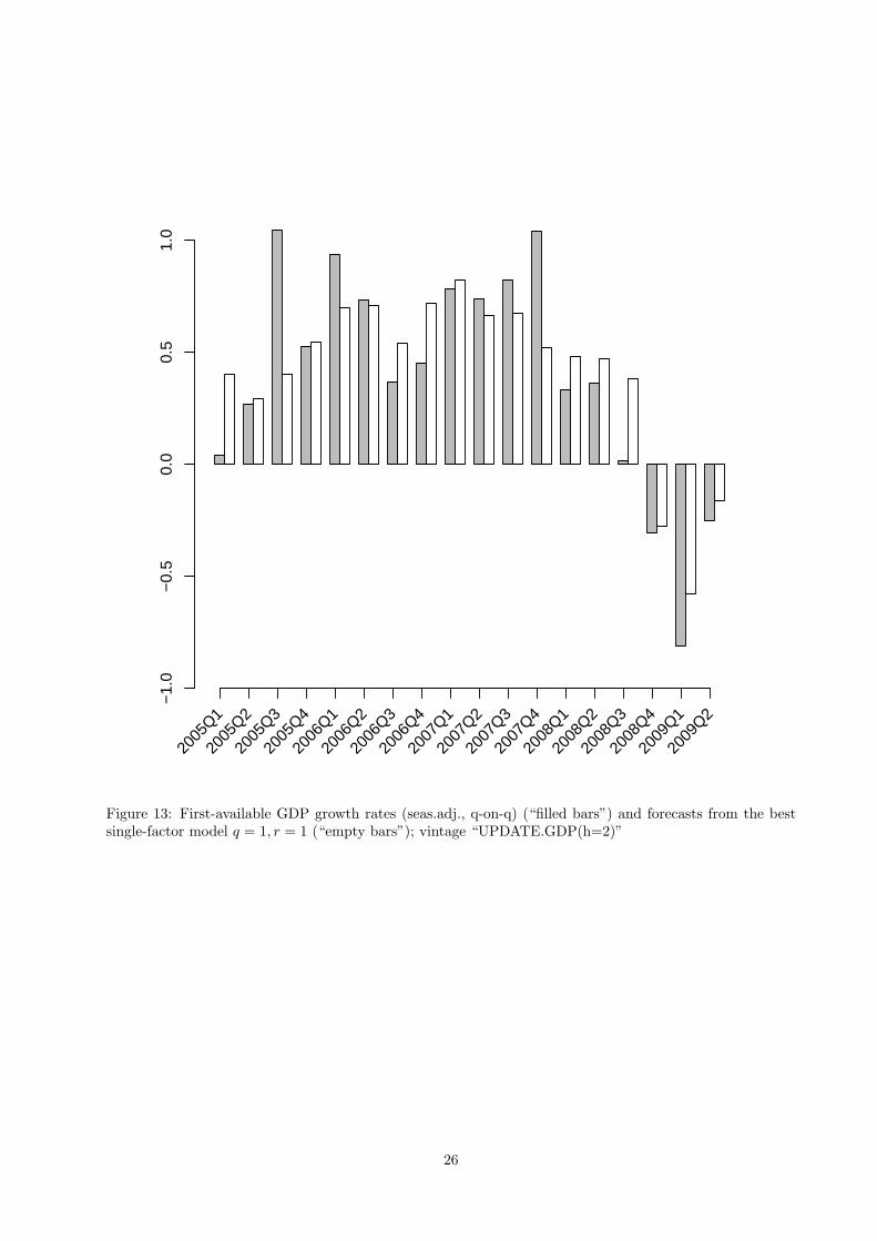
Finally, in Figure 13 we provide the actual values of the first release of the quarterly GDP and the

forecasts from the preferred model produced during the vintage “UPDATE.GDP(h=0)” that corresponds to

the lowest relative RMSFE observed, see Figure 7. The timing of this vintage is the very beginning of the last

month of forecast quarter corresponding to nowcasts. We find that our nowcasts can rather good trace the

actual growth rate. With respect to the predicting the current crisis we notice that our nowcasts correctly

predict the negative quarterly growth rates in the last three quarters—2008Q4, 2009Q1, and 2009Q2—of our

10

forecast sample, although it is slightly optimistic in 2008Q3. It is remarkable that the overall good nowcast

performance of the factor model has been achieved without any pre-selection of the indicators based, for

example, on correlation strength with the reference variable or any other pre-selection procedure suggested

in the literature (e.g., see Siliverstovs and Kholodilin, 2009; Bai and Ng, 2008; Boivin and Ng, 2006).

6 Conclusion

In this paper we utilize the dynamic factor model based on 562 monthly indicators for now-/forecasting the

quarter-on-quarter growth rates of seasonally adjusted GDP in Switzerland. To the best of our knowledge

our study represents the first attempt to employ this sort of models for predicting Swiss GDP. We find that

the preferred version of the dynamic factor model offers substantial improvement in forecast accuracy when

compared to that based on a naive constant-growth model. The highest forecast accuracy of the first official

release of GDP growth rates for an actual quarter is achieved about three months before the release takes

place. The corresponding ratio of the RMSFE of the factor model to that of the benchmark model is 49%.

Furthermore, we use the factor model in order to investigate the informational content of subsequent

data releases of various macroeconomic variables. To this end, we perform a pseudo-real-time exercise where

we simulate the asynchronous pattern of within-month releases of various blocks of data. We find that both

business tendency surveys and stock market indices have the most informational content for predicting GDP

in Switzerland. However, we must issue a warning here that the outcome in such exercises may crucially

depend on the applied transformation of the monthly indicators—a topic that, in our view, largely seems

to be overlooked in the routine applications involving large data sets. For example, we find that the largest

marginal impact on forecast accuracy is attributed to surveys in the model where the monthly indicator

were not subject to the end-of-quarter transformation. In the factor model where such transformation was

applied we find that the largest informational content is attributable to the stock market variables.

We also find out that different transformations of the variables may not only result in different ranking of

the importance of difference data blocks for forecasting GDP but also may influence the overall forecasting

performance of the factor model. Thus, for our data set at hand we find out that the best forecasting results

are achieved in the model where a single factor is extracted from the panel where the monthly survey indica-

tors did not undergo any transformation (neither stationarity-related nor end-of-quarter equivalents) whereas

the remaining blocks including the block of stock market indices undergo both types of transformation.

References

Aastveit, K. A. and T. G. Trovik (2007). Nowcasting Norwegian GDP: The role of asset prices in a small

open economy. Working Paper 2007/09, Norges Bank.

Artis, M., A. Banerjee, and M. Marcellino (2001). Factor forecasts for the UK. Economics Working Papers

ECO2001/15, European University Institute.

11

Bai, J. and S. Ng (2008). Forecasting economic time series using targeted predictors. Journal of Economet-

rics 146 (2), 304–317.

Boivin, J. and S. Ng (2006). Are more data always better for factor analysis? Journal of Economet-

rics 132 (1), 169–194.

Croushore, D. (2005). Do consumer-confidence indexes help forecast consumer spending in real time? The

North American Journal of Economics and Finance 16 (3), 435 – 450.

Diebold, F. X. and G. D. Rudebusch (1991). Forecasting output with the composite leading index : A

real-time analysis. Journal of the American Statistical Association 86 (415), 603–610.

Doornik, J. A. (2007). Object-Oriented Matrix Programming Using Ox. London: Timberlake Consultants

Press and Oxford: www.doornik.com.

Forni, M., M. Hallin, M. Lippi, and L. Reichlin (2000). The generalized dynamic-factor model: Identification

and estimation. The Review of Economics and Statistics 82 (4), 540–554.

Forni, M., M. Hallin, M. Lippi, and L. Reichlin (2005). The generalized dynamic factor model: One-sided

estimation and forecasting. Journal of the American Statistical Association 100, 830–840.

Giannone, D., L. Reichlin, and D. Small (2008). Nowcasting: The real-time informational content of macroe-

conomic data. Journal of Monetary Economics 55 (4), 665–676.

Graff, M. (2009). Does a multi-sectoral design improve indicator-based forecasts of the GDP growth rate?

Evidence for Switzerland. Applied Economics, forthcoming.

Kholodilin, K. A. and B. Siliverstovs (2006). On the forecasting properties of the alternative leading in-

dicators for the German GDP: Recent evidence. Journal of Economics and Statistics (Jahrbucher fur

Nationalokonomie und Statistik) 226 (3), 234–259.

Koop, G. and S. Potter (2004). Forecasting in dynamic factor models using Bayesian model averaging.

Econometrics Journal 7 (2), 550–565.

Muller, C. and E. Koberl (2008). Business cycle measurement: A semantic identification approach using

firm level data. Working paper 08-212, KOF Swiss Economic Institute, ETH Zurich.

Sancho, I. and M. Camacho (2002). Spanish diffusion indexes. Computing in Economics and Finance 2002

276, Society for Computational Economics.

Schumacher, C. (2007). Forecasting German GDP using alternative factor models based on large datasets.

Journal of Forecasting 26 (4), 271–302.

Schumacher, C. and J. Breitung (2008). Real-time forecasting of German GDP based on a large factor model

with monthly and quarterly data. International Journal of Forecasting 24 (3), 386–398.

12

Siliverstovs, B. (2009). Are business tendency surveys useful for short-term forecasting of GDP? Real-time

evidence for Switzerland. unpublished manuscript.

Siliverstovs, B. and K. A. Kholodilin (2009). On selection of components for a diffusion index model: It’s

not the size, it’s how you use it. Applied Economics Letters 16 (12), 1249–1254.

Stock, J. H. and M. W. Watson (2002a). Forecasting using principal components from a large number of

predictors. Journal of the American Statistical Association 97, 1167–1179.

Stock, J. H. and M. W. Watson (2002b). Macroeconomic forecasting using diffusion indexes. Journal of

Business and Economic Statistics 20 (2), 147–162.

13

0.00.20.40.60.81.0

EXC

H.R

ATE

PMG

RC

PI

LABO

URPP

I

CH

INO

GA

RET

AIL

TRAD

EST

MKT

INT.

RAT

E

EXC

H.R

ATE

PMG

RC

PI

LABO

URPP

I

CH

INO

GA

RET

AIL

TRAD

EST

MKT

INT.

RAT

E

EXC

H.R

ATE

UPD

ATE.

GD

P(h=

1)PM

GRC

PI

LABO

URPP

I

CH

INO

GA

RET

AIL

TRAD

EST

MKT

INT.

RAT

E

EXC

H.R

ATE

PMG

RC

PI

LABO

URPP

I

CH

INO

GA

RET

AIL

TRAD

EST

MKT

INT.

RAT

E

EXC

H.R

ATE

PMG

RC

PI

LABO

URPP

I

CH

INO

GA

RET

AIL

TRAD

EST

MKT

INT.

RAT

E

EXC

H.R

ATE

UPD

ATE.

GD

P(h=

0)PM

GRC

PI

LABO

URPP

I

CH

INO

GA

RET

AIL

TRAD

EST

MKT

INT.

RAT

E

EXC

H.R

ATE

h=2

h=1

h=0

Figure

1:RelativeRMSFE:Factor

modelq=

1,r=

1(w

ithou

tEQE-transformation)to

aconstant-grow

thmodel:2005Q1–2009Q2

14

0.00.20.40.60.81.0

EXC

H.R

ATE

PMG

RC

PI

LABO

URPP

I

CH

INO

GA

RET

AIL

TRAD

EST

MKT

INT.

RAT

E

EXC

H.R

ATE

PMG

RC

PI

LABO

URPP

I

CH

INO

GA

RET

AIL

TRAD

EST

MKT

INT.

RAT

E

EXC

H.R

ATE

UPD

ATE.

GD

P(h=

1)PM

GRC

PI

LABO

URPP

I

CH

INO

GA

RET

AIL

TRAD

EST

MKT

INT.

RAT

E

EXC

H.R

ATE

PMG

RC

PI

LABO

URPP

I

CH

INO

GA

RET

AIL

TRAD

EST

MKT

INT.

RAT

E

EXC

H.R

ATE

PMG

RC

PI

LABO

URPP

I

CH

INO

GA

RET

AIL

TRAD

EST

MKT

INT.

RAT

E

EXC

H.R

ATE

UPD

ATE.

GD

P(h=

0)PM

GRC

PI

LABO

URPP

I

CH

INO

GA

RET

AIL

TRAD

EST

MKT

INT.

RAT

E

EXC

H.R

ATE

h=2

h=1

h=0

Figure

2:RelativeRMSFE:Factor

modelq=

2,r=

2(w

ithou

tEQE-transformation)to

aconstant-grow

thmodel:2005Q1–2009Q2

15

0.0

0.4

0.8

PMGR CPI LABOUR PPI CHINOGA

0.0

0.4

0.8

CHINOGA

0.0

0.4

0.8

CHINOGA RETAIL TRADE

0.0

0.4

0.8

TRADE

0.0

0.4

0.8

TRADE STMKT

0.0

0.4

0.8

STMKT INT.RATE EXCH.RATE

Figure 3: Stationary monthly indicators (without EQE-transformation); Correlation with the first factor:2000M10–2009M6

16

0.0

0.4

0.8

PMGR CPI LABOUR PPI CHINOGA

0.0

0.4

0.8

CHINOGA

0.0

0.4

0.8

CHINOGA RETAIL TRADE

0.0

0.4

0.8

TRADE

0.0

0.4

0.8

TRADE STMKT

0.0

0.4

0.8

STMKT INT.RATE EXCH.RATE

Figure 4: Stationary monthly indicators (without EQE-transformation); Correlation with the second factor:2000M10–2009M6

17

0.0

0.4

0.8

PMGR CPI LABOUR PPI CHINOGA

0.0

0.4

0.8

CHINOGA

0.0

0.4

0.8

CHINOGA RETAIL TRADE

0.0

0.4

0.8

TRADE

0.0

0.4

0.8

TRADE STMKT

0.0

0.4

0.8

STMKT INT.RATE EXCH.RATE

Figure 5: Stationary monthly indicators (without EQE-transformation); Correlation with the third factor:2000M10–2009M6

18

0.00.20.40.60.81.0

EXC

H.R

ATE

PMG

RC

PI

LABO

URPP

I

CH

INO

GA

RET

AIL

TRAD

EST

MKT

INT.

RAT

E

EXC

H.R

ATE

PMG

RC

PI

LABO

URPP

I

CH

INO

GA

RET

AIL

TRAD

EST

MKT

INT.

RAT

E

EXC

H.R

ATE

UPD

ATE.

GD

P(h=

1)PM

GRC

PI

LABO

URPP

I

CH

INO

GA

RET

AIL

TRAD

EST

MKT

INT.

RAT

E

EXC

H.R

ATE

PMG

RC

PI

LABO

URPP

I

CH

INO

GA

RET

AIL

TRAD

EST

MKT

INT.

RAT

E

EXC

H.R

ATE

PMG

RC

PI

LABO

URPP

I

CH

INO

GA

RET

AIL

TRAD

EST

MKT

INT.

RAT

E

EXC

H.R

ATE

UPD

ATE.

GD

P(h=

0)PM

GRC

PI

LABO

URPP

I

CH

INO

GA

RET

AIL

TRAD

EST

MKT

INT.

RAT

E

EXC

H.R

ATE

h=2

h=1

h=0

Figure

6:RelativeRMSFE:Factor

modelq=

1,r

=1(w

ithEQE-transformation)to

aconstan

t-growth

model:2005Q1–2009Q2

19

0.00.20.40.60.81.0

EXC

H.R

ATE

PMG

RC

PI

LABO

URPP

I

CH

INO

GA

RET

AIL

TRAD

EST

MKT

INT.

RAT

E

EXC

H.R

ATE

PMG

RC

PI

LABO

URPP

I

CH

INO

GA

RET

AIL

TRAD

EST

MKT

INT.

RAT

E

EXC

H.R

ATE

UPD

ATE.

GD

P(h=

1)PM

GRC

PI

LABO

URPP

I

CH

INO

GA

RET

AIL

TRAD

EST

MKT

INT.

RAT

E

EXC

H.R

ATE

PMG

RC

PI

LABO

URPP

I

CH

INO

GA

RET

AIL

TRAD

EST

MKT

INT.

RAT

E

EXC

H.R

ATE

PMG

RC

PI

LABO

URPP

I

CH

INO

GA

RET

AIL

TRAD

EST

MKT

INT.

RAT

E

EXC

H.R

ATE

UPD

ATE.

GD

P(h=

0)PM

GRC

PI

LABO

URPP

I

CH

INO

GA

RET

AIL

TRAD

EST

MKT

INT.

RAT

E

EXC

H.R

ATE

h=2

h=1

h=0

Figure

7:RelativeRMSFE:Factormodel

withou

t(“filled

bars”)an

dwith(“em

pty

bars”)

EQE-transform

ation:2005Q1–2009Q2

20

0.0

0.4

0.8

PMGR CPI LABOUR PPI CHINOGA

0.0

0.4

0.8

CHINOGA

0.0

0.4

0.8

CHINOGA RETAIL TRADE

0.0

0.4

0.8

TRADE

0.0

0.4

0.8

TRADE STMKT

0.0

0.4

0.8

STMKT INT.RATE EXCH.RATE

Figure 8: Stationary monthly indicators (with EQE-transformation); Correlation coefficient larger than 0.60with the first factor: 2000M10–2009M6

21

0.0

0.4

0.8

PMGR CPI LABOUR PPI CHINOGA

0.0

0.4

0.8

CHINOGA

0.0

0.4

0.8

CHINOGA RETAIL TRADE

0.0

0.4

0.8

TRADE

0.0

0.4

0.8

TRADE STMKT

0.0

0.4

0.8

STMKT INT.RATE EXCH.RATE

Figure 9: Stationary monthly indicators (without EQE-transformation); Correlation coefficient larger than0.60 with the first factor: 2000M10–2009M6

22

0.00.20.40.60.81.0

EXC

H.R

ATE

PMG

RC

PI

LABO

URPP

I

CH

INO

GA

RET

AIL

TRAD

EST

MKT

INT.

RAT

E

EXC

H.R

ATE

PMG

RC

PI

LABO

URPP

I

CH

INO

GA

RET

AIL

TRAD

EST

MKT

INT.

RAT

E

EXC

H.R

ATE

UPD

ATE.

GD

P(h=

1)PM

GRC

PI

LABO

URPP

I

CH

INO

GA

RET

AIL

TRAD

EST

MKT

INT.

RAT

E

EXC

H.R

ATE

PMG

RC

PI

LABO

URPP

I

CH

INO

GA

RET

AIL

TRAD

EST

MKT

INT.

RAT

E

EXC

H.R

ATE

PMG

RC

PI

LABO

URPP

I

CH

INO

GA

RET

AIL

TRAD

EST

MKT

INT.

RAT

E

EXC

H.R

ATE

UPD

ATE.

GD

P(h=

0)PM

GRC

PI

LABO

URPP

I

CH

INO

GA

RET

AIL

TRAD

EST

MKT

INT.

RAT

E

EXC

H.R

ATE

h=2

h=1

h=0

Figure

10:RelativeRMSFE:Factor

modelsq=

2,r

=2(“filled

bars”)an

dq=

1,r

=1(“em

pty

bars”)

(withEQE-transform

ation):

2005Q1–2009Q2

23

0.00.20.40.60.81.0

EXC

H.R

ATE

PMG

RC

PI

LABO

URPP

I

CH

INO

GA

RET

AIL

TRAD

EST

MKT

INT.

RAT

E

EXC

H.R

ATE

PMG

RC

PI

LABO

URPP

I

CH

INO

GA

RET

AIL

TRAD

EST

MKT

INT.

RAT

E

EXC

H.R

ATE

UPD

ATE.

GD

P(h=

1)PM

GRC

PI

LABO

URPP

I

CH

INO

GA

RET

AIL

TRAD

EST

MKT

INT.

RAT

E

EXC

H.R

ATE

PMG

RC

PI

LABO

URPP

I

CH

INO

GA

RET

AIL

TRAD

EST

MKT

INT.

RAT

E

EXC

H.R

ATE

PMG

RC

PI

LABO

URPP

I

CH

INO

GA

RET

AIL

TRAD

EST

MKT

INT.

RAT

E

EXC

H.R

ATE

UPD

ATE.

GD

P(h=

0)PM

GRC

PI

LABO

URPP

I

CH

INO

GA

RET

AIL

TRAD

EST

MKT

INT.

RAT

E

EXC

H.R

ATE

h=2

h=1

h=0

Figure

11:RelativeRMSFE:Factor

modelsq=

2,r

=1(“filled

bars”)an

dq=

1,r

=1(“em

pty

bars”)(w

ithEQE-transform

ation):2005Q1–2009Q2

24

2005 2006 2007 2008 2009

−0.

50.

00.

51.

0

zoo.

fcst

0.00

0.04

0.08

0.12

2005

Q1

2005

Q2

2005

Q3

2005

Q4

2006

Q1

2006

Q2

2006

Q3

2006

Q4

2007

Q1

2007

Q2

2007

Q3

2007

Q4

2008

Q1

2008

Q2

2008

Q3

2008

Q4

2009

Q1

2009

Q2

Figure 12: Vintages-specific forecasts from the best single-factor model q = 1, r = 1 (the upper panel);Variance across all vintage-specific forecasts for a given quarter (the lower panel)

25

−1.

0−

0.5

0.0

0.5

1.0

2005

Q1

2005

Q2

2005

Q3

2005

Q4

2006

Q1

2006

Q2

2006

Q3

2006

Q4

2007

Q1

2007

Q2

2007

Q3

2007

Q4

2008

Q1

2008

Q2

2008

Q3

2008

Q4

2009

Q1

2009

Q2

Figure 13: First-available GDP growth rates (seas.adj., q-on-q) (“filled bars”) and forecasts from the bestsingle-factor model q = 1, r = 1 (“empty bars”); vintage “UPDATE.GDP(h=2)”

26

Table 1: Chronology of data releases during the month

Block Published by Timing (approx.) Publication lag Block size(in months)

PMGR-manufacturing Credit Suisse 1st working 1 9day of month

CPI Swiss Federal Statistical Office First week of month 1 28Labour State Secretariat for Economic Affairs Second week of month 1 6PPI Swiss Federal Statistical Office Second week of month 1 13BTS in manufacturing KOF Swiss Economic Institute Middle of month 0 150Retail Swiss Federal Statistical Office Middle of month 2 4Exports/Imports Swiss Federal Customs Administration Middle of month 1 249Stock market indices Datastream Last day of month 0 80

(monthly average)Interest rates Datastream Last day of month 0 20

(monthly average)Exchange rates Datastream Last day of month 0 3

(monthly average)

The chronological sequence of block releases has been recorded in October 2009. We proceed under assumption that such orderingand timing has been constant over time. However, we readily acknowledge that the actual timing and ordering may slightly vary.

27