Assessing uncertainty in fuzzy land cover classification ... · Assessing uncertainty in fuzzy land...

INTERNATIONAL JOURNAL OF GEOMATICS AND GEOSCIENCES

Volume 5, No 2, 2014

© Copyright by the authors - Licensee IPA- Under Creative Commons license 3.0

Research article ISSN 0976 – 4380

Submitted on August 2014 published on November 2014 332

Assessing uncertainty in fuzzy land cover classification by confusion index Ganesh Prasad M.S1, Manoj K. Arora2

1- Professor, Department of Civil Engineering, The National Institute of Engineering,

Mysore, India

2- Director, PEC University of Technology, Chandigarh, India

[email protected], [email protected]

ABSTRACT

In recent years, uncertainty has become an important subject in assessing the quality of

remote sensing image classification. Classification uncertainty is due to poor class definition,

transition zones and the presence of mixed pixels in remote sensing data. Fuzzy classification

approaches aim to estimate the proportions of specific classes that occur within each pixel.

Partial class membership values derived from fuzzy classification serve as baseline

information to assess classification uncertainties and allow the depiction of spatial variation

of uncertainty. Providing uncertainty information at pixel level may assist in increasing the

confidence in using thematic maps produced from remote sensing image classification. Many

metrics have been developed to quantify pixel-wise classification uncertainty. In the present

study, two formulations of confusion index are used. Literature state that, the two forms of

confusion index provide similar information. The present study aims at examining whether

these two formulations provide similar information or not. Multispectral image from Landsat-

7 ETM+ sensor was subjected to fuzzy c-means classification. The derived class membership

values for each pixel were used in quantifying classification uncertainty. A comparative

analysis of classification uncertainty provided by two forms of confusion index was carried

out. The results from the study show that the two forms of confusion index provide dissimilar

information on classification uncertainty.

Keywords: Remote sensing, Fuzzy classification, Quality, Uncertainty, Confusion index

1. Introduction

Remote sensing from satellite based sensors provides synoptic views of the earth surface at

regular time intervals, and has been considered as an attractive source of data acquisition.

Transformation of observed remote sensing data in the form of spectral responses into

thematic classes representing earth surface features is achieved by a number of image

classification procedures. Digital image classification in supervised mode is generally used to

produce land use and land cover maps from remotely sensed data. A conventional statistical

classifier like maximum likelihood classifier (MLC) allocates each pixel in the image to one

of the classes in which it has the highest probability of membership. The uses of such ‘hard’

or ‘crisp’ classification methods are only appropriate when the classes are discrete and

mutually exclusive. However, most of the land use/land cover features are continuous rather

than discrete. Classifying continuous features as discrete may result in loss of information

about the spatial distribution of a thematic class.

Fuzzy logic introduced by Zadeh (1965) can be used to classify and assess continuous

thematic classes. The use of fuzzy classification to produce accurate and reliable land cover

maps is gaining importance due to its continuous nature of class representation. Fuzzy

Assessing uncertainty in fuzzy land cover classification by confusion index

Ganesh Prasad M.S and Manoj K. Arora

International Journal of Geomatics and Geosciences

Volume 5 Issue 2, 2014 333

classification is a quantitative, iterative method for classifying thematic classes as continuous

over geographic space. Fuzzy classification approaches aim to estimate the proportions of

specific classes that occur within each pixel.

It has been reported that fuzzy classification approaches provide a general though not optimal

solution to mixed pixel problem. The strong relationship between fuzzy membership values

and true proportions of land cover classes has been supported by Maselli et al. (1994),

Atkinson et al. (1997), Deer and Eklund (2003). Further, extraction of class proportions in a

pixel through fuzzy classification facilitates to derive information on classification

uncertainties that are beyond the possibilities of conventional error matrix approach. This has

been advantageous to users who are in need of uncertainty information for their specific

applications and to indicate the quality of classification.

In recent years, uncertainty has become an important subject in remote sensing and has

attracted attention of many researchers (Canters, 1997; Kiiveri, 1997; Heuvelink, 1998;

Foody, 2002) and is a key issue in data quality assessment. Providing uncertainty

information at pixel level may assist in increasing the confidence in using thematic maps

produced from digital classification of remote sensing data.

This paper attempts to quantify classification uncertainty associated with an image pixel

using two measures suggested by Burrough et al. (1997). A comparison of results obtained

from these two measures is also made. For the purpose, class membership values derived

from fuzzy –c means classification of Landsat ETM+ data is used. This paper is organized

into four sections. The next section briefly discusses the experimental data used. Section 3

describes fuzzy classification of experimental data and subsequent estimation of classification

uncertainty using two forms of confusion index. In Section 4, a comparison of two forms of

confusion index is made based on experimental results and hypothetical examples. Finally,

summary and conclusions are provided in Section 5.

2. Experimental data description

The remote sensing data considered for this study is a multi-spectral image from Landsat-7

ETM+ sensor, which acquires data in eight spectral bands . The size of the image considered

for this study is 327 x 221 pixels, with spatial resolution of 30 meter, covering a part of

Syracuse city area in U.S.A. Although, the sensor acquires the data in different spectral bands,

only six are considered here, since the spatial resolutions of panchromatic (band 8) and

thermal infrared band (band 6) are different from other bands. Of the 6 bands available , three

bands viz. band 2 (0.52-0.6 µm), band 3 (0.63-0.69 µm) and band 5 (1.55-1.75 µm ) were

selected for classification purpose.

Transformed divergence was used in this study to select the best set of bands from

multispectral images. Transformed divergence (TD) was computed based on the training

data statistics. The larger the TD, the greater is the separation between the training signatures

of those classes. A TD value of 2000 suggests an excellent separability; a value of 1900

provides good separation and values less than 1700 represent poor separability between

classes (Jensen, 1986). From the transformed divergence analysis conducted on all the six

bands in synthetic and remote sensing dataset, a TD value of 2000 was obtained for the

combination of bands 2, 3 and 5. Therefore, these three bands were used as input into the

classifier selected for deriving class membership values.

Figure 1 shows the false colour composite (FCC) of the image of the study area. The central

portion of the image consists of urban area, whereas, remaining portion of the image is

mostly covered by vegetation. The urban area also covers a diverse environment including





lakes, parks, residential area, vegetation and roads, thereby introducing spatial complexity

due to class mixture and overlapping, and thus may be regarded as area with high uncertainty

in class allocation. Keeping in view the diverse environmental characteristics of the study

area, five major land cover classes were selected. These classes include, trees, grass, bare

soil, water and impervious. The characteristics of these classes are given in Table 1.

In the present data set, for example, the classes, trees and grass generally tend to overlap due

to spectral similarities. Further, the class impervious which consists of buildings, roads etc.,

may sometimes include the other class viz., bare soil. This overlapping of class definition

introduces uncertainty in class allocation. Moreover, the data itself consists of large quantity

of mixed pixels (about 45%), which contribute to the aspects of classification uncertainty to a

large extent.

Table 1: Characteristics of major thematic classes in the study area

Thematic classes considered for

classification

Description

Trees Forest, variety of native plants

Grass Open space, shrubs, golf course,

play grounds, parks, lawns

Bare soil Exposed soil surfaces, patches

Water Lakes, ponds, channels

Impervious Residential area, major and minor

roads, open roof

Figure 1: False colour composite of the Landsat ETM+ sensor data

(Red: band 5, Green: band 3, Blue: band 2)

3. Fuzzy classification

Fuzzy c-means classifier (FCM) described by Bezdek et al. (1984) was adopted to classify

the study image. This algorithm has proven especially popular (Legleiter and Goodchild,

2005: Bastin, 1997: Wu and Yang, 2002: Yang et al., 2003) and has been used to produce

land cover maps from remotely sensed data (Zhang and Stuart, 2001). In most of the

situations the FCM classifier may be advantageous (Shalan et al., 2003) as it is not dependent





on the data distributional assumptions. The fuzzy membership values derived from FCM

range between 0 (no membership) and 1 (full membership) and specify the degree of

belongingness of a pixel to a specific class. Although, FCM is an unsupervised classifier

(Bezdek et al., 1984) it may be used in supervised mode (Key et al., 1989: Foody, 2000).

Fuzzy c-means algorithm is an iterative clustering algorithm which subdivides data into c-

clusters or classes. The algorithm is based on iterative optimization of an objective function

Jm, which is a generalised least squared errors function and is defined as (Bezdek, 1981),

( ) ∑ −∑==

=c

k A

mN

jm vxJ kjjkXVU

1

2

1

)(:, µ (1)

where U is a fuzzy c partition of dataset X containing N pixels.

xj = vector denoting spectral response of a pixel j

c = fixed and known number of clusters in X ;

m = weighting exponent or fuzzy exponent; 1 ≤ m ≤ ∞ which defines the degree of fuzziness

(µ jk)m = the mth power of xj s membership in cluster k.

V is the collection of cluster centres vk, ║xj–vk║2A is the squared distance djk between xj and vk

with )()(2

2vxvxvxd kj

T

Ajk Akjkj −== −−

where A = positive definite weight matrix

Given the values of c and m, the algorithm iteratively assigns pixels to clusters and

recalculates cluster centres until Jm achieves a local minimum. The fuzzy partition U =

[ µ jk ] is referred to as the grade of membership of xj to the cluster k with µ jk ∈ [0, 1] .

The formulation of FCM contains a weighting factor m, which describes the degree of

fuzziness to be provided in the classification. The value of m varies from 1 (no fuzziness or

hard classification) to ∞ (complete fuzziness), however a value in the range of 1.5 to 3 may

be generally adopted (Shalan et al., 2003). Through several experiments, a value of 2.0 was

found to be suitable for the classification of this dataset. The number of training samples were

201, 172, 31, 204 and 296 for the classes trees, grass, bare soil, water and impervious

respectively. In this study, FCM classification in supervised mode using Euclidean distance

metric has been performed on PARBAT (www.lucieer.net, 2014), a public domain software

for advanced remote sensing image processing and visual fuzzy classification.

The results of the classification were five fraction images (Figure 2 (a) to (e)) corresponding

to five land cover classes considered in the experiment. In Figure 2(a) to (e), bright pixels

indicate higher class membership values. And, darker pixels correspond to lower values of

class membership. When each pixel is assigned to the class to which it has the highest

membership, the result is a ‘defuzzified’ or ‘hardened’ image equivalent to a classified image.

The defuzzified image is shown in Figure 2 (f). As expected the two classes trees and grass

overlapped in the outer portion of the image (See Figure 2), where as the class water is

correctly classified. However, the class impervious tends to get mixed up with other classes

viz. trees and grass. A small amount of overlap is also observed between the classes bare soil

and impervious.





(a) Trees (b) Grass

(b) Bare soil (d) Water

(e) Impervious (f) Defuzzified image

Figure 2: Class membership images (fraction images) derived from FCM classification

(fuzzy exponent m =2) and defuzzified image showing thematic classes.

3.1 Classification Uncertainty

The main idea of fuzzy classification approach is to associate a pixel with every class

considered in the classification scheme, with variable degree of class memberships. Partial

class membership values derived from fuzzy classification can serve as baseline information

to assess classification uncertainties and allow the depiction of spatial variation of

uncertainty. To elaborate this, if we consider the output of a fuzzy classifier for a given pixel,

the output is a finite set of class membership values. Larger is the set of membership values

for a pixel, lesser is the precision of information available and higher is the ambiguity.

Further, for some regions class membership values may be equal or nearly equal in a pixel.

The more similar the membership values for two or more classes, the greater the confusion

about to which class a pixel actually belongs. In such cases too, it is not clear that which class

dominates and may lead to a state of ambiguity. In such a situation, the ambiguity in class

assignment can be represented by measures such as entropy (Maselli et al., 1994), Quadratic

score (Glasziou and Hilden, 1989: Fatemi et al., 2004 ), non- specificity, U-uncertainty

(Dubois and Prade, 1987: Ricotta, 2005) and confusion index (Burrough et al., 1997). In the

present study, a measure of ambiguity viz. confusion index in difference and ratio forms

suggested by Burrough et al., (1997) is considered for the quantification of classification

uncertainty.





Let µjk

be the class membership value of jth pixel in kth class, with k = 1,2,…. n classes,

and 10 ≤≤ µjk

with the normalization constraint of 11

=∑=

n

kjk

µ ,which is generally imposed in

fuzzy classification. Further, let { }n

jjjjC µµµµµ .,.........,,)(321

= be an ordered (in descending

order) fuzzy set having class membership values of a pixel j in which the numbers 1,2…n

indicate first highest membership, second highest membership ( µn

j will obviously be

minimum).

Consider the first and second highest class membership values µ1

j, µ

2

j for a pixel j. The

difference between these two is an indirect representation of conflict in assigning the pixel to

one of the classes. For example, if the difference is large, it is an indication of lesser conflict.

On the other hand, a difference of zero or near zero indicates high degree of conflict. Let the

difference between the first and second highest membership values be D, given by

D = ( µ1

j- µ

2

j ) (2)

Normalizing the difference with the maximum membership value and deducting it from the

total membership of one, yields a measure of confusion as,

Measure of confusion = µ

µµ

max

21)(

1jj

−− (3)

where µmax is the maximum class membership value for the pixel j. The denominator in the

second term, i.e., µmax can take two values. A value of 1, which is the limiting value of

membership or the maximum class membership value as derived from classification process.

When the second term in Eq. (3) is normalized with respect to µmax

=1, the measure of

confusion will be equal to 1 - ( µ1

j- µ

2

j ). When it is normalized with respect to maximum

membership value for the pixel, i.e., µ1

j, the measure of confusion will be equal to

µ

µ1

2

j

j.

Burrough et al., (1997) provided these two formulations (Eq. (4) and (5)) and termed both as

confusion index (CI).

µ

µ1

2

j

jCI = (4)

)(121

µµ jjCI −−= (5)

CI can take values between 0 and 1. If CI → 0, then one class dominates and there is little

confusion in allocating pixel to that class and the degree of uncertainty is low. If CI → 1, then

both µ1

j and µ

2

j are equal or near equal and there is maximum confusion about the class to

which the pixel belongs and the degree of uncertainty is high. Ideally, in a land use/land

cover map derived from FCM classification, the zones represented by those pixels with CI

values equal to 1 or nearly 1 would indicate the geographic boundaries between fuzzy classes.

Burrough et al., (1997), while providing the two formulations of CI, stated that these two

produce similar results. Legleiter and Goodchild (2005) termed these two formulations (Eq. 4

and Eq. 5) as ratio (CIratio) and difference (CIdifference) forms of confusion index. and utilized

them to derive maps of classification uncertainty to identify heterogeneous and complex areas.





However, it is not known whether these two formulations produced similar maps of

classification uncertainty.

Anomalies can be observed in depicting the quality of classification based on uncertainty

estimated using two forms of confusion index. For instance, consider one of the cases where

the highest membership value µ1

j = 0.4 and the second highest membership value µ

2

j = 0.15

for a pixel. The value of uncertainty estimated for this case by the ratio form of confusion

index is 0.375, while it is equal to 0.75 by the difference form of confusion index. If the ratio

form of confusion index is used to represent classification uncertainty, the value of 0.375 for

this pixel can generally be considered as low. Correspondingly, if one wants to express the

quality of classification based on uncertainty, a value of 0.375 does not draw much attention.

On the other hand, if the difference form of confusion index is used for the same pixel,

uncertainty value of 0.75, which is twice that of the value provided by CIratio, is considered as

a high value and hence the thematic quality of the pixel may be treated as significantly

ambiguous. Due to these anomalies between the two forms of confusion index, quality

assessment process itself may be dubious. Therefore, this study aims at comparing the

results obtained from the two formulations of confusion index. Such a comparative

evaluation of two forms of confusion indices may help in understanding their behaviour and

relative efficacies.

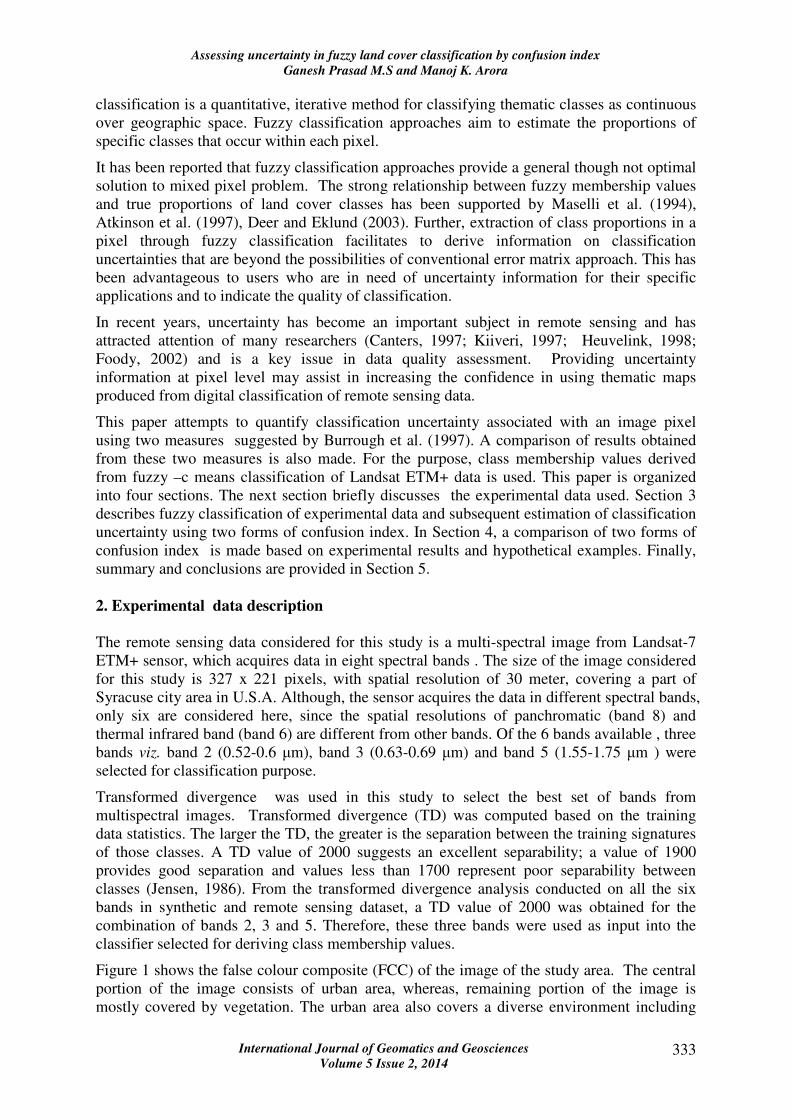
To quantify classification uncertainty, the derived fuzzy membership values have been

arranged in descending order (i.e., images showing the highest membership values, second

highest membership values and third highest membership values etc.) and have been used as

input to computational models. Based on the formulations for confusion index CI (Eq. 4 and

Eq. 5), classification uncertainty maps were generated for the study area. Figures 3 and 4

show spatial pattern of classification uncertainty for the experimental image using two

formulations of CI. In these uncertainty images, dark pixels indicate the regions classified

with no or minimum uncertainty, whereas brighter pixels indicate uncertain classification or

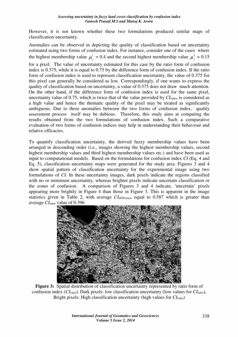
the zones of confusion. A comparison of Figures 3 and 4 indicate, ‘uncertain’ pixels

appearing more brightly in Figure 4 than those in Figure 3. This is apparent in the image

statistics given in Table 2, with average CIdifference equal to 0.587 which is greater than

average CIratio value of 0.396.

Figure 3: Spatial distribution of classification uncertainty represented by ratio form of

confusion index (CIratio). Dark pixels: low classification uncertainty (low values for CIratio),

Bright pixels: High classification uncertainty (high values for CIratio)





Figure 4: Spatial distribution of classification uncertainty represented by difference form of

confusion index (CIdifference). Dark pixels: low classification uncertainty (low values for

CIdifference), Bright pixels: High classification uncertainty (high values for CIdifference)

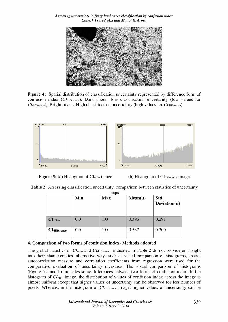
Figure 5: (a) Histogram of CIratio image (b) Histogram of CIdifference image

Table 2: Assessing classification uncertainty: comparison between statistics of uncertainty

maps

Min Max Mean(µ) Std.

Deviation(σ)

CIratio 0.0 1.0 0.396 0.291

CIdifference 0.0 1.0 0.587 0.300

4. Comparison of two forms of confusion index- Methods adopted

The global statistics of CIratio and CIdifference indicated in Table 2 do not provide an insight

into their characteristics, alternative ways such as visual comparison of histograms, spatial

autocorrelation measure and correlation coefficients from regression were used for the

comparative evaluation of uncertainty measures. The visual comparison of histograms

(Figure 5 a and b) indicates some differences between two forms of confusion index. In the

histogram of CIratio image, the distribution of values of confusion index across the image is

almost uniform except that higher values of uncertainty can be observed for less number of

pixels. Whereas, in the histogram of CIdifference image, higher values of uncertainty can be





observed for sufficiently large quantity of pixels. This is augmented by the global statistics of

CIratio and CIdifference images (Table 2). Although, the range of these two metrics is the same

i.e., 0 to 1, the mean value of CIratio is 0.396 and it is equal to 0.587 for CIdifference image.

This disparity is pointing towards lower values of CIratio for pixels in ambiguous zones and

higher values of CIdifference for the same pixels. Higher values for CIdifference may be due to the

fact that CIdifference is the result of aggregation of CIratio and another measure of class

membership saturation viz. Exaggeration uncertainty (Zhu, 1997) using a fuzzy operator (

Ganesh Prasad and Arora, 2008).

A linear regression was carried out to understand the relation between two forms of confusion

index. The correlation coefficient between CIratio and CIdifference was found to be 0.81

indicating the absence of perfect correlation between them. Since, this regression was carried

out on pixel by pixel basis for two values given by CIratio and CIdifference, a comparison based

on the spatial dependency of uncertainty could not be achieved. Therefore, spatial

autocorrelation analysis was carried out to explore the spatial dependency between pixels

based on the values of uncertainty.

4.1 Comparison based on spatial autocorrelation

Spatial autocorrelation refers to the effect that a certain characteristic at a given location has

on that same characteristic at neighbouring locations. In other words, given a group of

mutually exclusive units in a two dimensional plane, if the presence, absence or degree of a

certain characteristic affects the presence, absence or degree of the same characteristic in

neighbouring units, then the phenomenon is said to exhibit spatial autocorrelation (Cliff and

Ord, 1973). Spatial autocorrelation analysis examines whether the observed value of a

variable at a location is independent of the values of the variable at neighbouring locations. If

dependence exists, the variable is said to exhibit spatial autocorrelation. This spatial

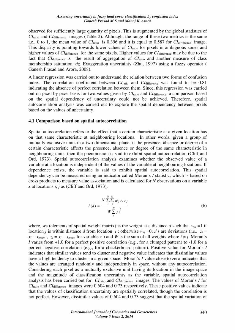
dependency can be measured using an indicator called Moran’s I statistic, which is based on

cross products to measure value association and is calculated for N observations on a variable

x at locations i, j as (Cliff and Ord, 1973),

∑

∑∑

=N

i

N

i

N

jjiij

z

zzw

iW

N

dI2

)( (6)

where, wij (elements of spatial weight matrix) is the weight at a distance d such that wij =1 if

location j is within distance d from location i ; otherwise wij =0; z’s are deviations (i.e., zi =

xi – xmean , zj = xj – xmean for variable x ) and W is the sum of all weights where i ≠ j. Moran’s

I varies from +1.0 for a perfect positive correlation (e.g., for a clumped pattern) to -1.0 for a

perfect negative correlation (e.g., for a checkerboard pattern). Positive value for Moran’s I

indicates that similar values tend to cluster and negative value indicates that dissimilar values

have a high tendency to cluster in a given space. Moran’s I value close to zero indicates that

the values are arranged randomly and independently in space, without any autocorrelation.

Considering each pixel as a mutually exclusive unit having its location in the image space

and the magnitude of classification uncertainty as the variable, spatial autocorrelation

analysis has been carried out for CIratio and CIdifference images. The values of Moran’s I for

CIratio and CIdifference images were 0.604 and 0.73 respectively. These positive values indicate

that the values of classification uncertainty are spatially correlated, though the correlation is

not perfect. However, dissimilar values of 0.604 and 0.73 suggest that the spatial variation of





CIratio is different than CIdifference . The results from visual comparison of uncertainty maps,

image histograms and correlation analysis have pointed towards a clear distinction between

the information on uncertainty conveyed by the two forms of confusion index. Although,

Burrough et al., (1997) stated that two forms of confusion index produce similar results, it

does not appear so as indicated here.

4.2 Comparison based on zonation

From the hypothetical example discussed in 3.1, it is evident that under certain situations

there occurs a considerable difference between two forms of confusion index. Therefore, in

order to verify whether the anomaly between two forms of confusion index is significant for a

dataset, a simple approach has been adopted here. In this approach, the pixels have been

grouped into four qualitative zones. This has been done using two criteria.

Criterion I: Four qualitative zones corresponding to low, medium, high and very high values

of confusion index have been considered. These four zones correspond to the values in the

range (0.0 - 0.25), (0.25 to 0.50), (0.50 to 0.75) and (0.75 to 1.0). This zonation was done

arbitrarily. The percentage of pixels in each zone is represented in Figure 6. In medium and

high zones of uncertainty the variation between CIratio and CIdifference is 8.67% and 6.52%

respectively. In the zone of low uncertainty CIratio has 20.17% pixels more than CIdifference ,

where as CIdifference has 22.31% more pixels than CIratio in the zone of very high uncertainty.

Criterion II: In this approach, zonation is made based on image statistics of CIratio and

CIdifference i.e., mean (µ) and standard deviation (σ). Percentage of pixels with low

uncertainty (≤(µ - σ)), medium ((µ - σ) to µ), high (µ to (µ + σ)) and very high uncertainty (>

(µ + σ)) are represented in Figure 7.

In the zone of low uncertainty the variation between CIratio and CIdifference is less and is equal

to 0.13% , whereas in the zone of high uncertainty the variation is 1.78% only. In the zone of

medium uncertainty CIratio has 10.99% pixels more than CIdifference , where as CIdifference has

12.9% more pixels than CIratio in the zone of very high uncertainty.

Figure 6: Comparison of CIratio and CIdifference based on number pixels in each of the

four bins of equal size





Figure 7: Comparison of CIratio and CIdifference based on number pixels in each of the

four bins of unequal size

Therefore, from the results obtained by the comparison of percentage of pixels in different

zones (low, medium, high and very high) based on the values of CIratio and CIdifference (criteria

I and II), it is evident that the two forms of confusion index behave differently for a given

classification.

From this analysis, it is observed that the difference exists in the depiction of quality of a

pixel using ratio and difference forms of confusion index both qualitatively and spatially.

Therefore, the information on classification uncertainty in the form of confusion as expressed

by the two forms of confusion index is considered as different and the two forms of confusion

index does not provide similar results as stated by Burrough et al.,(1997).

5. Summary and conclusions

Uncertainty plays a vital role in land use land cover classification of remotely sensed data.

When the remotely sensed data to be classified consists of abundant mixed pixels and /or

overlapping classes for example, different types of vegetation, classification of such an image

results in high degree of uncertainty. Fuzzy classification of land use/land cover provides a

framework that allows partial memberships in multiple classes and gradual transition between

fuzzy classes, which can be considered as an advantage over conventional crisp classification.

Class membership values derived from FCM classification are used to quantify pixel wise

classification uncertainty, which further be used to represent spatial pattern of classification

uncertainty. Uncertainty maps thus generated are useful in identifying and quantifying areas

of high/low classification reliability. Burrough’s confusion index (CI) used in this study can

be appropriate in knowing to what extent the spatial distribution of thematic classes derived

from fuzzy classification is ambiguous. The objective of this paper is to compare

classification uncertainty maps derived from two formulations of confusion index. Although,

the two forms of confusion index are intended to provide similar information, certain

situations may exist when these two exhibit considerable difference. A comparative analysis





of classification uncertainty provided by two forms of confusion index is carried out. The

result from the study shows that the two forms of confusion index provide dissimilar

information on classification uncertainty both quantitatively and spatially. It is difficult to

suggest any one form of confusion index measure as appropriate or ideal measure of

classification uncertainty. However, it is concluded here that the selection of an appropriate

measure of classification uncertainty may be made by considering the factors viz., quantity of

mixed pixels present in the image to be classified, the type of uncertainty to be represented

and the theoretical framework of uncertainty measure.

6. References

1. Atkinson, P.M., Cutler, M.E.J., and Lewis, H., 1997, Mapping sub-pixel proportional

land cover with AVHRR imagery, International Journal of Remote Sensing, 18, pp

917-935.

2. A-Xing Zhu, 1997, Measuring uncertainty in class assignment for natural resource

maps under fuzzy logic, Photogrammetric Engineering and Remote Sensing, 63(10),

pp 1195-1202.

3. Bastin, L., 1997, Comparison of fuzzy c-means classification, linear mixture

modelling and MLC probabilities as tools for unmixing coarse pixels, International

Journal of Remote Sensing, 18(17), pp 3629-3648.

4. Bezdek, J.C., Ehrlich, R. and Full, W., 1984, FCM: The fuzzy c-means clustering

algorithm, Computers and Geosciences, 10, pp 191-203.

5. Burrough, P.A., Van Gaans, P.F.M., and Hootsmans, R., 1997, Continuous

classification in soil survey: spatial correlation, confusion and boundaries, Geoderma,

77, pp 115-135.

6. Canters F., 1997, Evaluating the uncertainty of area estimates derived from fuzzy land

cover classification, Photogrammetric Engineering and Remote Sensing, 63(4), pp

403-414.

7. Cliff, A.D., Ord, J.K., (1973), Spatial Autocorrelation (London: Pion Limited)

8. Deer, P.J., Eklund,P., 2003, A study of parameter values for a Mahalanobis distance

fuzzy classifier, Fuzzy Sets and Systems, 137, pp 191-213.

9. Dubois, D. and Prade, H., 1987, Properties of measures of information in evidence

and possibility theories, Fuzzy Sets and Systems, 24, pp 161-182.

10. Fatemi, S.B., Mojaradi B. and Varshosaz., 2004, "Introducing an accuracy indicator

based on uncertainty related measure", XXth ISPRS Congress, Istanbul, Turkey,

Commission 4, pp 974-979.

11. Foody, G.M., 2000, Estimation of sub-pixel land cover composition in the presence of

untrained classes, Computers and Geosciences, 26, pp 469-478.

12. Foody, G.M., 2002, Status of land cover classification accuracy assessment, Remote

Sensing of Environment, 80, pp 185-201.





13. Glasziou, P. and Hilden, J., 1989, Test selection measures, Medical Decision

Making, 9, pp 133-141.

14. Heuvelink, G.B.M., (1998), Error Propagation in Environmental Modelling with GIS.

Taylor and Francis, London.

15. Jensen, J.R., (1986). Introductory Digital Image processing, Prentice-Hall, NJ.

16. Key, J.R., Maslanik, J.A., Barry, R.G., 1989, Cloud classification from satellite data

using a fuzzy sets algorithm: a polar example, International Journal of Remote

Sensing, 10(12), pp 1823-1842.

17. Kiiveri H.T., 1997, Assessing, representing and transmitting positional uncertainty in

maps, International Journal of Geographic Information Science, 11(1), pp 33-52.

18. Legleiter, C.J., Goodchild, M.F., 2005, Alternative representations of in-stream

habitat: classification using remote sensing, hydraulic modeling, and fuzzy logic,

International Journal of Geographical Information Science, 19(1), pp 29-50.

19. Lucieer, A., (2004), Parbat-a software tool for segmentation and explorative

visualization of remotely sensed imagery. URL: http://parbat.lucieer.net

20. Mark Gahegan, Manfred Ehlers, 2000, A frame work for the modelling of uncertainty

between remote sensing and geographic information systems, ISPRS Journal of

Photogrammetry and Remote Sensing, 55, pp 176-188.

21. Maselli, F., Conese, C., And Petkov, L., 1994. Use of probability entropy for the

estimation and graphical representation of the accuracy of maximum likelihood

classification, ISPRS Journal of Photogrammetry and Remote Sensing, 49, pp 13-20.

22. Ricotta, C., 2005, On possible measures for evaluating the degree of uncertainty of

fuzzy thematic maps, International Journal of Remote Sensing, 26, pp 5573-5583.

23. Shalan, M. A., Arora, M. K., and Ghosh, S. K., 2003, An evaluation of fuzzy

classifications from IRS 1C LISS III imagery : a case study, International Journal of

Remote Sensing, 24, pp 3179-3186.

24. Wu, K.L., Yang, M.S., 2002, Alternative c-means clustering algorithms, Pattern

Recognition, 35, pp 2267-2278.

25. Yang, M.S., Hwang, P.Y., Chen, D.H., 2003, Fuzzy clustering algorithms for mixed

feature variables, Fuzzy Sets and Systems, 141, pp 301-317.

26. Zadeh, L.A., 1965, Fuzzy sets, Information Control, 8, pp 338-353.

27. Zhang, J., Stuart, N., 2001, Fuzzy methods for categorical mapping with image based

land cover data, International Journal of Geographic Information Science, 15(2), pp

175-195.

Date post:	02-Aug-2018
Category:	Documents
Upload:	vukhuong
View:	216 times
Download:	0 times

Assessing uncertainty in fuzzy land cover classification ... · Assessing uncertainty in fuzzy land...

Documents