Assessing uncertainty on Net-to-gross at the Appraisal Stage:

Application to a West Africa Deep-Water Reservoir

Amisha Maharaja

April 25, 2006

Abstract

A large data set is available from a deep-water reservoir offshore West Coast ofAfrica. The objective of this study is to assess the uncertainty about the net-to-gross(NTG) ratio of this reservoir by mimicking appraisal stage conditions. Early strati-graphic interpretation is retained and two different depositional facies scenarios areconsidered. The structural setting is well-known, hence the uncertainty about the ge-ological scenario is mostly related to facies distribution. A prior NTG distribution isobtained from a database of analog reservoirs. Four wells, those available at appraisalstage, and acoustic impedance data are retained for the uncertainty study. The NTGuncertainty workflow is carried out using two different geological scenarios to updatethe prior NTG distribution into two posterior distributions.

The posteriors obtained from using the two geological scenarios are similar becausethe two scenarios are not very different from the perspective of NTG uncertainty. Bothscenarios are conditioned to the same set of data and the same prior NTG distributionwas used, which further diminishes the difference between the two scenarios. The im-pact of additional data is investigated by conducting the study with one well and thenrepeating it each time a new well is added. With each additional well the posteriorNTG distribution becomes narrower, which implies that additional data is reducing theuncertainty interval. The posterior NTG distribution with twenty-eight wells, whichprovide a good coverage of the reservoir, is very narrow and has a mean comparable tothe mean of the posterior with the four appraisal stage wells. This suggests that thepay zones in this reservoir are not localized vertically.

1 Introduction

Hydrocarbon exploration is a risky business. Apart from the economical and geo-politicalfactors, early estimates about the reserves is a major source of uncertainty. In expensive,deepwater reservoirs it is crucial to know very early the distribution of hydrocarbon in place(HIP) in the reservoir before expensive development costs are committed.

The uncertainty about the gross reservoir volume has the first order impact on the HIPcalculations. The volume uncertainty, however, is related to seismic data processing andinterpretation, which falls outside the scope of this research. We assert that the net-to-gross(NTG) ratio of a hydrocarbon reservoir has the next crucial impact on the HIP calculations.A workflow, based on Bayesian framework, was proposed by Caumon et al. (2004) to assess

1

uncertainty about the NTG ratio. This workflow identifies (a) the geological scenario, (b)prior NTG distribution and (c) the quantitative data themselves as the major sources ofuncertainty related to NTG.

In this paper we apply this workflow to a real reservoir from off-shore West Coast ofAfrica (WCA). The reservoir will be refered to as the WCA reservoir in the paper. Thegoal is to use only the data available at the appraisal stage, assess the uncertainty aboutthe NTG and compare the results with the NTG obtained from a dense well data set fromthe same reservoir. First we recall the basic framework of the workflow. Next, we describein section 2 the two alternative geological scenarios, the prior NTG distribution and theavailable quantitative data. We aim to study the impact of geological scenario, the impactof introducing additional well data and the impact of using seismic data on the posteriorNTG distribution. The results are discussed in section 4 and we draw some conclusions insection 5.

1.1 Review of methodology

Net-to-Gross is defined as the ratio of volume of reservoir quality rock to total rock volumein the reservoir. By definition this is a global parameter and it has no replicate. Someresearchers have used spatial boostrap as a way to assess uncertainty about the NTG es-timate by randomizing the well data location and re-sampling from stochastic realizations(Journel, 1993; Norris et al., 1993; Bitanov and Journel, 2004). However, stochastic simu-lation requires a model of spatial variability and a prior knowledge of NTG value, both ofwhich are highly uncertain.

Caumon et al. (2004) realized this problem and proposed to randomize both, the geolog-ical scenario and the prior global NTG value. We denote the uncertain geological scenarioby S, with sk, k = 1, . . . , K being its realizations. At the appraisal stage, if the geologicalsetting is poorly understood, it is essential to consider different geological scenarios that fitall available data until some could be eliminated by subsequently acquired data.

The prior global NTG value is also casted as a random variable (RV) denoted A. Thetrue, but unknown, NTG value of the reservoir is a realization of this RV. The quantitativedata are treated as a realization of the RV data, denoted D. Spatial bootstrap addressesthe uncertainty about the observed data. By framing the problem in this manner, Caumonet al. (2004) ask the question, what is the uncertainty about the global NTG value giventhe observed data and geological interpretation. Since it is not practical to compute thelikelihood of all available data, we retain the NTG estimate, A⋆, as a summary of the data.

The proposed workflow is summarized in (Figure 1). Refer to Caumon et al. (2004)for details on the theoretical foundations of this workflow. Associated with each geologicalscenario, S = sk, is a prior distribution of NTG values, P (A|S = sk), see Figure 1, Panel A.This prior distribution would be typically drawn from the company prior expertise aboutthis type of geological scenario. To update this distribution into a posterior distributiongiven a NTG estimate, P (A|S = sk, A

⋆ = a⋆0), the workflow proceeds as follows:

2

• The prior NTG distribution is discretized into M classes resulting in M realizationsof the NTG, a1, . . . , aM (Figure 1, Panel B).

• Corresponding to each class of NTG, L realizations of the reservoir facies are generatedusing some simulation algorithm, preferably one that utilizes multiple-point statisticsbecause it is better at honoring the data patterns found in the geological scenario.

• Freezing the seismic data and initial drilling strategy, N sets of synthetic wells aresampled from the L realizations by randomizing the well locations. This provides N ∗L

realizations of the NTG estimate, a⋆1, . . . , a⋆

NL. From this distribution the likelihoodof observing the initial best NTG estimate for the given class of true NTG and givengeological scenario, P (A⋆ = a⋆

0| A = am, S = sk), is obtained (Figure 1, Panel C).

• Bayes inversion is then used to obtain the probability of the true NTG being in thatclass given the observed NTG estimate and geological scenario, P (A = am | A⋆ =a⋆

0, S = sk) (Equation 1).

P (A = am | A⋆ = a⋆0, S = sk) =

P (A⋆ = a⋆0| A = am, S = sk) ∗ P (A = Am | S = sk)

P (A⋆ = a⋆0| S = sk)

(1)The denominator P (A⋆ = a⋆

0| S = sk) is obtained by applying the total probability

rule (2).

P (A⋆ = a⋆0 | S = sk) =

M∑

m=1

P (A⋆ = a⋆0 | A = am, S = sk) ∗ P (A = am | S = sk) (2)

• This procedure, when repeated for each class of true NTG, gives the posterior distri-bution of true NTG given the initial NTG estimate for a given geological scenario,P (A = am | A⋆ = a⋆

0, S = sk) (Figure 1, Panel D).

• If desired, the probability distribution for the true NTG given initial best estimate,P (A = am | A⋆ = a⋆

0), can be obtained using the total probability rule (3).

P (A = am | A⋆ = a⋆0) =

K∑

k=1

P (A = am | A⋆ = a⋆0, S = sk) ∗ P (S = sk) (3)

Assigning a prior probability P (S = sk) to a geological scenario is necessarily asubjective task. A convenient alternative to using expert knowledge is to assume eachscenario to be equally likely, which might be reasonable in sparse data situation.

To summarize, Caumon et al. (2004) considered three jointly related sources of uncer-tainty: the geological scenario S, the true NTG value A, and the global NTG estimate A⋆

obtained from the available data. Seismic data, the well-to-seismic calibration algorithm,and the initial drilling strategy are frozen throughout, however these can be randomized ina broader study.

3

2 Information available at appraisal stage

2.1 Geological scenarios

At the appraisal stage the degree of uncertainty about the geological setting depends onseveral factors. If the reservoir is located in a frontier basin the uncertainty tends to bemuch higher as opposed to a mature basin where the geological setting is known with greaterconfidence. In deep-water settings the quality of seismic data also plays a big role. Well-imaged seimic data can significantly reduce the uncertainty about the structural settingand, in exceptionally good cases, even the facies types can be deduced from the seismicamplitude slices. Conversely, poorly imaged seismic data can lead to higher uncertaintyabout both, the reservoir boundaries and the facies types. In most cases the quality ofseismic data falls somewhere in between these two extremes.

In the WCA reservoir the seismic data quality is sufficiently good to identify the struc-tural setting with a high degree of confidence. It is determined to be a Slope-Valley (SV)system from the very get-go. However, the internal complexity of this SV system has in-creased with time as the seismic data was better interpreted. It is observed that the greaterthe number of mapped geobodies, the smaller the gross reservoir volume, and consequentlythe smaller the OOIP. For this study we retain the appraisal stage stratigraphic architectureas shown in Figure 2. Figure 2(a) shows a schematic of the reservoir boundaries interpretedfrom the seismic data and Figure 2(b) shows the corresponding reservoir grid. The entireworkflow is limited to this domain.

The depositional facies within the SV region, however, cannot be easily inferred fromthe seismic data. Since the structural setting is known in this case, the uncertainty aboutgeological setting boils down to the uncertainty about the type and distribution of thedepositional facies. This facies uncertainty is expressed through different training images(Ti). From well-log analysis four depositional facies were identified. The NTG ratio withinthese facies are given in Table 1. Facies 1, which has the lowest NTG, is the backgroundfacies. Facies 4, with the highest NTG, is interpreted as channels and it is the mainreservoir rock. The Tis can be divided into two families depending on how facies 3 and4 are characterized. In the first family of scenarios, facies 2 with 47.3 percent NTG ischaracterized as poor quality channels, and facies 3 with 63.0 percent NTG is consideredas intermediate quality channels (Figure 3). In the second set of scenarios, facies 2 andfacies 3 have been interpreted as poor and intermediate quality lobes respectively (Figure4). The within-family scenarios differ from one another with respect to channel widths,width-to-depth ratio, and channel sinuosity. To study the impact of geological scenario, onerepresentative Ti is retained from each of the two family of Tis. Figure 5 shows these twoscenarios.

2.2 Prior knowledge of net-to-gross distribution

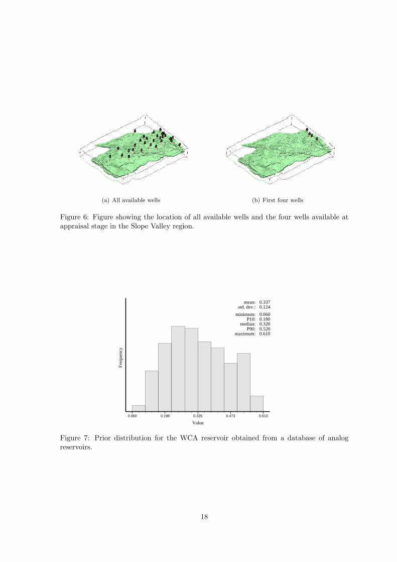
A prior NTG distribution for the WCA reservoir is obtained using a database of analogreservoirs. This distribution is shown in Figure 7. The bounds of the distribution, [0.06,0.61], specify the minimum and maximum NTG values expected to be found in a reservoir

4

like the WCA reservoir. In the Bayesian framework adopted in this workflow the bounds ofthe posterior distribution cannot be greater than those of the prior distribution, hence it isadvisable to choose a conservative (i.e. wide) prior distribution.

Note that the prior distribution is defined independently from the actual data from theWCA reservoir. It is obtained by pooling together information from other reservoirs thatare deemed analogous to the WCA reservoir; hence it is truly a prior in the Bayesian sense.The goal of the workflow is to update this prior distribution taking account of actual quan-titative data available on the WCA reservoir. In the analog database system used for thisstudy, the reservoirs are classified at the system scale and not based on the depositionalfacies. In the WCA reservoir since the structural style is unambiguously determined to beSlope Valley, only one prior NTG distribution was available for the different facies scenarios.Ideally, each geological scenario should have a different prior NTG distribution.

Since the prior NTG distribution is independent from the local reservoir data, it doesnot change as new data becomes available. However, if the interpretation of the geologicalscenario changes as a result of new data, then a new prior distribution may have to beconsidered.

2.3 Well and seismic data

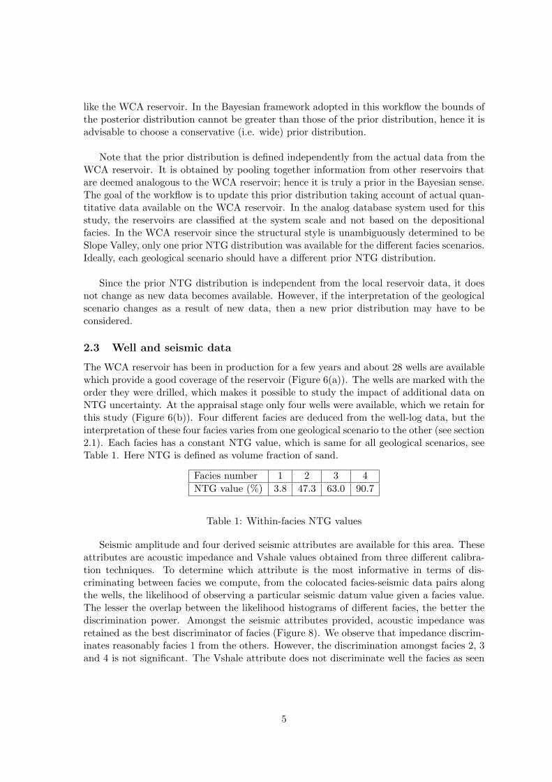
The WCA reservoir has been in production for a few years and about 28 wells are availablewhich provide a good coverage of the reservoir (Figure 6(a)). The wells are marked with theorder they were drilled, which makes it possible to study the impact of additional data onNTG uncertainty. At the appraisal stage only four wells were available, which we retain forthis study (Figure 6(b)). Four different facies are deduced from the well-log data, but theinterpretation of these four facies varies from one geological scenario to the other (see section2.1). Each facies has a constant NTG value, which is same for all geological scenarios, seeTable 1. Here NTG is defined as volume fraction of sand.

Facies number 1 2 3 4

NTG value (%) 3.8 47.3 63.0 90.7

Table 1: Within-facies NTG values

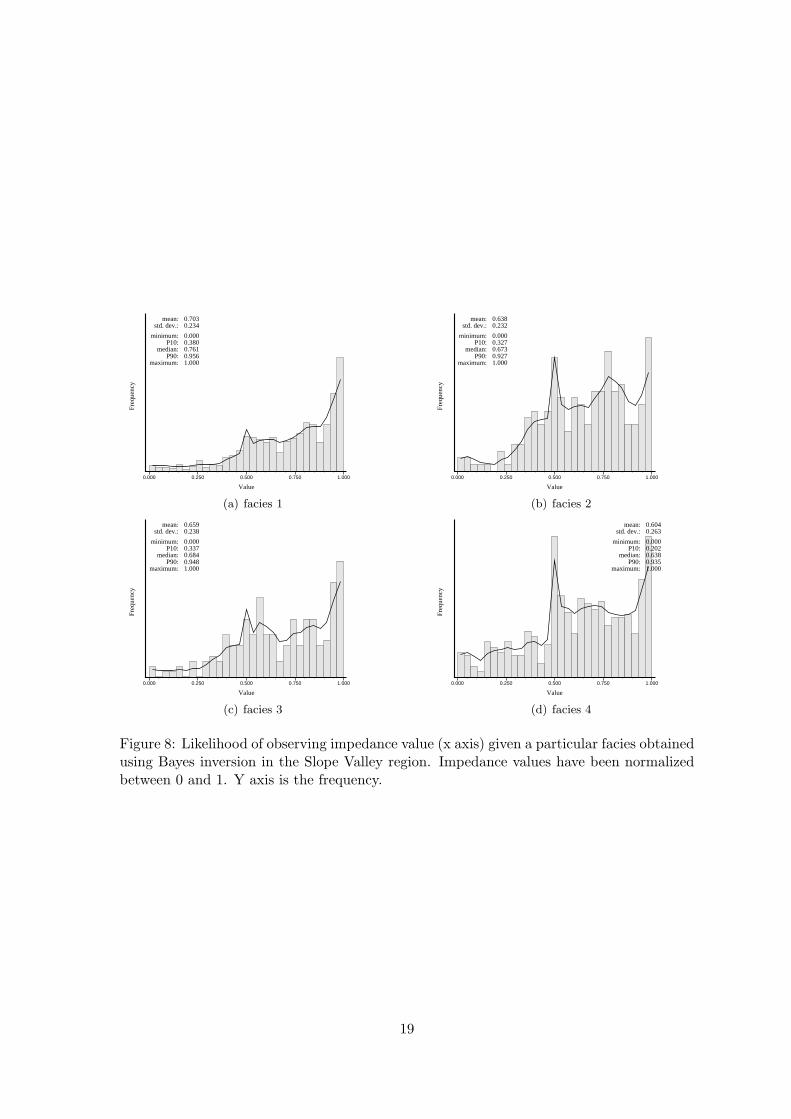
Seismic amplitude and four derived seismic attributes are available for this area. Theseattributes are acoustic impedance and Vshale values obtained from three different calibra-tion techniques. To determine which attribute is the most informative in terms of dis-criminating between facies we compute, from the colocated facies-seismic data pairs alongthe wells, the likelihood of observing a particular seismic datum value given a facies value.The lesser the overlap between the likelihood histograms of different facies, the better thediscrimination power. Amongst the seismic attributes provided, acoustic impedance wasretained as the best discriminator of facies (Figure 8). We observe that impedance discrim-inates reasonably facies 1 from the others. However, the discrimination amongst facies 2, 3and 4 is not significant. The Vshale attribute does not discriminate well the facies as seen

5

from the seismic likelihoods (Figure 9). For this study we retain the acoustic impedance(AI) for NTG computations.

3 NTG estimation

At an appraisal stage wells are few and they tend to be preferentially located. This is truefor the WCA reservoir (Figure 6(b)), hence the NTG estimate retained from the four clus-tered wells might not be representative of the entire reservoir. Seismic data, on the otherhand, informs the entire area. If seismic is informative and properly calibrated with thereservoir facies, then a seismic-based NTG estimate would be closer to the true reservoirNTG value. Several techniques for integrating seismic data with facies exists in literature(Fournier and Derain, 1995; Goovaerts, 1997; Caers and Ma, 2002; Strebelle et al., 2002).The major stumbling block for many of these techniques is that they might not be robust insparse data situation such as this. A simpler, but robust method, would be more suitablefor this situation. Bayes inversion, as used by (Bitanov and Journel, 2004), is retainedto calibrate seismic data with facies in this paper. Note that the conceptual frameworkpresented here does not call for any specific calibration technique.

Essentially in the Bayes inversion method, the colocated facies-impedance pairs are usedto compute the likelihood of observing impedance values given a facies category,P (S = sj | F = fi). The facies proportions computed from wells are used as the priorfacies proportion, P (F = fi). For each facies category, Bayes inversion is then applied ateach grid location, u, to compute the probability of observing a facies category given theobserved impedance value at that location (Equation 4). Here, n refers to the number offacies and m is the total number of classes into which the seismic data is discretized whencomputing its likelihood probability from the well data. In Equation 4, P (F = fi) is theproportion of facies i from the wells. Hence, Equation 4 can be interpreted as the updateof well facies proportions using seismic data.

P (F (u) = fi | S(u) = sj ) =P (S = sj | F = fi) × P (F = fi)

P (S = sj); i = 1, . . . , n; j = 1, . . . , m

(4)By performing Bayes inversion at each grid location for the n facies categories we get n

facies probability 3D maps; the average of these 3D maps is the updated proportion pi foreach facies i (Equation 5).

pi =

n∑

i=1

P (F = fi(u) | S = sj(u) ) (5)

If the calibration is properly done and the seismic data are informative, we expect thatthese updated proportions would be more representative of the true facies proportions inthe reservoir than the well facies proportions. Table 2 gives the proportions of the fourfacies from wells and the updated proportions after integrating acoustic impedance withthe well facies data.

Notice that the proportion of facies 4, which is has highest NTG ratio has gone down,while that of facies 1, which is the low NTG background facies has gone up. This implies

6

Facies number 1 2 3 4

Well propotions 0.63 0.10 0.06 0.21

Updated proportions 0.66 0.09 0.06 0.18

Table 2: Facies proportions observed along the wells and after integrating well data withacoustic impedance data.

that the initial wells were preferentially located in higher pay zone. Without the correctioninduced by seismic data the reservoir NTG would be over estimated from the sole well data.Equation 6 is used to compute NTG by combining the updated facies proportions pi andthe within-facies NTG values ni given in Table 1 under the constraint that the proportionssum to one.

a⋆ =∑

(pi × ni) ;∑

pi = 1 (6)

The well NTG estimate and the updated NTG estimate after integrating acoustic impedancedata are given in Table 3.

Data NTG estimate

4 wells 0.484

4 wells + AI 0.436

Table 3: NTG estimate from wells and after integrating well and acoustic impedance data.

Consider the reverse situation when the global NTG value and the within-facies NTGvalues ni are known and we need to compute the proportion of each facies. In the twofacies case Equation 6 is sufficient to compute the facies proportions because we have twounknowns and two constraints. However, for more than two facies we have fewer constraintsthan unknowns and it is not possible to compute facies proportions unless additional con-straints are introduced to match the number of unknowns.

We propose to freeze the ratio of facies proportions as additional constraints. For exam-ple consider the four facies in a fluvial reservoir. By freezing the channel to levee ratio andthe channel to crevasse ratio, we can eliminate two unknowns, i.e. the proportion of leveeand crevasse, and solve for channel and floodbasin proportions using Equation 6. Once theproportion of channel is known, we can easily retrieve the proportions of levee and crevasse.The ratios to be frozen are uncertain parameters; they can be read from a training image,an outcrop or analog reservoirs or from geological expertise. This approach works best whenthe facies proportions are related as in the fluvial case. In case of the WCA, we froze thefacies 2 to facies 4 proportions ratio and that between facies 3 and facies 4. These ratioswere read from the Ti, see Table 4.

7

Facies # 1 2 3 4

Ti1 0.51 0.10 0.09 0.30

Ti2 0.50 0.11 0.09 0.30

Table 4: Facies proportion found in Ti1 (Figure 5(a)) and Ti2 (Figure 5(b)).

4 Results and Discussion

4.1 Impact of geological scenario

The goal of this section is to understand how the uncertainty on the geological scenarioaffects the posterior NTG distribution. In case of the WCA reservoir the main source ofgeological uncertainty is related to the type of depositional facies. As discussed in section2.1 we retain the two scenarios shown in Figure 5 as representatives from the two families ofscenarios. The NTG uncertainty workflow is carried out twice, first using the Ti1 (Figure5(a)), then using Ti2 (Figure 5(b)). All other parameters of the workflow were frozen;see Table 5 for details. The NTG values within each facies (Table 1) are held constantthroughout the study and the same values are used for both scenarios.

Parameter Value Parameter Value

Wells 4 Well NTG 0.48

Seismic data Acoustic Impedance Nb secondary classes 15

Prior NTG distribution from database Nb of NTG classes 10

Nb of realizations 1 Nb of resamplings 500per classes per class

Minimum interdistance 200 m Preferential Nobetween wells resampling

Table 5: Key parameters of the NTG uncertainty workflow used to study the impact ofgeological scenario uncertainty on posterior NTG distribution.

The posteriors obtained using Ti1 and Ti2 given a NTG estimate of 0.436 (see Table 3)are shown in Figure 10. Selected statistics of these two posteriors are summarized in Table6.

Geol Scenario Mean [p10, p90]

Ti1 0.377 [0.312, 0.451]

Ti2 0.379 [0.308, 0.454]

Table 6: Statistics of the posterior NTG distribution obtained using the two geologicalscenarios, Ti1 (Figure 5(a)), and Ti2 (Figure 5(b)).

The first thing to notice is that the two posteriors are very similar; their posterior sta-tistics differ only in the third decimal. This is also observed for posteriors obtained using

8

different number and location of wells. This leads to the conclusion that the two geolog-ical scenarios retained, though different in some of their depositional facies, are not verydifferent from the perpective of NTG uncertainty. The main reservoir facies is similar inboth scenarios and the relative proportion of facies is also similar. Moreover, the same priorNTG distribution was used for both scenarios, which further reduces the difference betweenthe two posteriors.

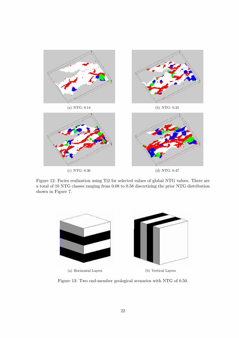
Figures 11 and 12 show some realizations generated using the two training images forselected classes of global NTG. Notice how in both cases the channel continuity is better re-produced as the global NTG ratio becomes higher. This is a limitation of the multiple-pointsimulation algorithm snesim; in low NTG cases it is difficult to reproduce thin, connectedfacies such as channels. Using a Ti that is several times larger than the simulation domainwould help improve this continuity. Moreover, in this case a strong servo-system control isused to exactly reproduce the desired global facies proportions. When the Ti facies propor-tions are drastically different from the target simulation proportions a strong servo-systemcorrection is needed to enforce the reproduction of these target proportions, at the costof deviating from the Ti structures thus leading to poor structure reproduction. A betteralternative is to build, for each global NTG class, a Ti whose facies proportions are reason-ably close to the desired target proportions.

In terms of spatial distribution of the reservoir rock the two scenarios are also very similarbecause the channel sands are distributed fairly uniformly in the reservoir, i.e. the sandsare not localized. Consequently, the impact of geological scenario uncertainty as assessedthrough spatial boostrap is low. Consider for example the two end-member scenarios shownin Figure 13; both scenarios have the same global NTG of 0.50. In Figure 13(a), the sandand shale layers are horizontally stacked hence any vertical well would sample exactly theglobal NTG value. On the other hand, in Figure 13(b) the sand and shale layers arevertically stacked, hence the NTG of any vertical well would be either 0 or 1 and the NTGestimate on an average would be 0.50. In this latter case the uncertainty about the NTGestimate is much higher and is dependent on the number of wells. Figure 14 shows thespatial bootstrap histograms corresponding to these two scenarios using 1, 2 and 4 wellsrespectively. Both scenarios are stationary, but in the vertically stacked case uncertaintyabout the NTG estimate is much higher. If horizontal wells were used the results would bereversed.

4.2 Impact of prior NTG distribution

As mentioned in section 2.2, only one prior NTG distribution is available for the two geo-logical scenarios because, in the analog database system used for this study, the reservoirsare classified at the system scale and not based on the depositional facies. Ideally, eachgeological scenario should have a different prior distribution associated with it. Since, wedo not have an alternate prior NTG distribution for the WCA reservoir, we retain a uniformprior distribution over [0.06, 0.61] and run the workflow with Ti1 to study the impact ofprior distribution on posterior NTG distribution. Note that the bounds of this uniform dis-tribution are the same as that of the prior distribution obtained from the analog database,

9

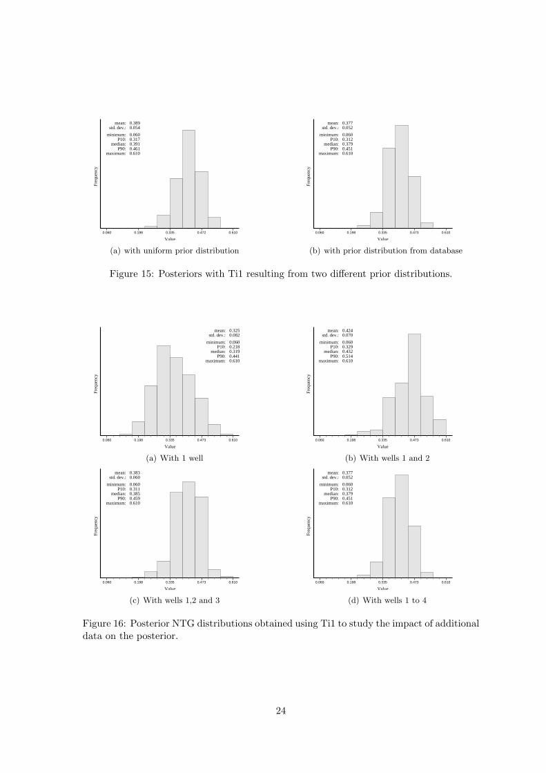
however, this is an extreme distribution because it implies that each class of NTG betweenits bounds is equally likely. The summary statistics of the two prior distributions and theirresulting posterior distributions are give in Table 7.

Distribution Mean [p10, p90]

Uniform prior 0.335 [0.115, 0.555]

Analog prior 0.337 [0.180, 0.520]

Posterior from 0.389 [0.317, 0.461]Uniform prior

Posterior from 0.377 [0.312, 0.451]Analog prior

Table 7: Summary statistics of two prior NTG distributions and their corresponding pos-terior distributions for scenario Ti1 (Figure 5(a)).

Figure 15 compares the posteriors resulting from using the two different prior distrib-utions. Note that the initial NTG estimate, 0.436, is identical in both cases because thesame set of four initial wells and acoustic impedance data are retained. We notice thatthe [p10, p90] interval corresponding to the posterior distribution resulting from the uniformprior is slightly wider than that of the posterior resulting from the prior distribution shownin Figure 7. Also, the posterior distribution corresponding to the uniform prior distributionis more symmetric than the latter posterior distribution. Both these observations also applyto the prior distributions, which suggests that the shape and range of the prior distributiondoes impact the resulting posterior distribution. Indeed, recall that the prior probabilityof the global value being in a certain class given a geological scenario, P (A = am|S = sk),impacts the posterior probability P (A = am|A⋆ = a⋆, S = sk) through Equation 1.

4.3 Impact of additional data

The impact of additional data on the posterior NTG distribution is studied using only theTi1 scenario, since both Ti1 and Ti2 give similar posterior distributions. The goal is to seehow the posterior NTG distribution changes as we add new well data. We perform the entireworkflow four times, first using only well 1, then adding well 2, then well 3 and finally withall four initial wells. The only parameters that change from one run to another are the initialNTG estimates and the number of wells used for spatial bootstrap. Table 8 summarizes thewell NTG and the updated NTG estimates after integration of acoustic impedance data.The resulting posterior NTG distributions are shown in Figure 16; summary statistics aregiven in Table 8.

First thing we notice is that the [p10, p90] interval of the posterior distribution withthe first well (Figure 16(a)) is much narrower than that of the prior NTG distribution(Figure 7. The posterior distribution mean and the [p10, p90] interval shifts to the rightwhen well 2 is introduced (Figure 16(b)) because the combined NTG estimate of wells 1and 2 is much higher than that of well 1. Also, the [p10, p90] interval of the posterior withtwo wells is narrower than that with well 1 only. This trend is also observed when wells3 and 4 are introduced. In all four cases the [p10, p90] interval is roughly centered over

10

Nb wells Well NTG Updated NTG Posterior mean Posterior [p10, p90]

1 0.355 0.351 0.325 [0.218, 0.441]1,2 0.471 0.450 0.424 [0.329, 0.514]1,2,3 0.472 0.428 0.383 [0.311, 0.459]1,2,3,4 0.483 0.436 0.377 [0.312, 0.451]

Table 8: Well NTG and the corresponding updated NTG estimates for wells 1 to 4. Theupdated estimates are retained for the study.

the corresponding mean as expected. The initial NTG estimates (Table 8) are includedin all posterior [p10, p90] intervals. The mean and the [p10, p90] intervals of the posteriordistributions are strongly impacted by the initial NTG estimate as demonstrated by thisstudy. Hence, when estimating NTG it is paramount to carefully choose the estimationfunction and consider all available data while accounting for errors in data, data uncertaintyand the redundancy between different data.

4.4 Impact of seismic data

The four initial wells are used to study the impact of seismic data on the posterior NTGdistribution. The workflow is run twice, once using acoustic impedance and once withoutusing it. Ti1 (Figure 5(a)) and the prior distribution shown in Figure 7 are used for bothruns. Table 9 gives the initial NTG estimate and the posterior statistics resulting from thetwo runs. The resulting posterior distributions are shown in Figure 17.

with seismic (AI) without seismic

Well NTG 0.483 0.483Initial estimate 0.436 0.483Posterior mean 0.391 0.472Posterior [p10, p90] [0.324, 0.457] [0.404, 0.539]

Table 9: Posterior NTG distribution statistics with Ti1 using four initial wells, with andwithout using acoustic impedance data.

When seismic data is not used the initial estimate is the same as the well estimate.Integrating seismic data lowers the estimate which indicates that the initial four wells werepreferentially located. Comparing the posterior distribution in Figure 17(a) with that inFigure 17(b) we observe that the posterior [p10, p90] interval widths are comparable in thetwo cases, however, the [p10, p90] without seismic is shifted to the right as the initial NTGestimate without seismic data is higher. Note that in both cases the initial estimate isincluded in the posterior [p10, p90] and this interval is roughly centered around the posteriormean.

11

4.5 Comparison with dense well data

When studing the NTG uncertainty for real reservoirs like the WCA, we do not have theluxury of knowing the true NTG value unlike in synthetic examples. However, we do haveat later times dense well data set that provides a good coverage of the WCA reservoir, seeFigure 6(a) for the location of all 28 wells. The 28 well NTG estimate and the integratedNTG estimate are given in Table 10 along with the estimates from the four initial wells.We notice that after integrating seismic data the 28 well NTG estimate is only slightlylowered. This suggests that these wells sample the reservoir NTG reasonably well. Also,notice that the NTG estimate from the initial, clustered, four wells is not too far from theestimate from all 28 wells. This implies that the pay zones in the reservoir are reasonablywell distributed such that even a few clustered wells are able to sample the global NTGvalue fairly closely; see Figure 13 and refer to the corresponding discussion in section 4.1.

4 initial wells All 28 wells

Well NTG 0.483 0.432Initial estimate 0.436 0.415Posterior mean 0.391 0.399Posterior [p10, p90] [0.324, 0.457] [0.363, 0.428]

Table 10: Comparison of posterior NTG distribution statistics resulting from using theinitial four wells and all 28 wells from the reservoir. Ti1 and the prior distribution shownin Figure 7 are used in both cases.

Figure 18 compares the posterior distributions resulting from using only the four initialwells and then using all 28 wells. The means of the two posterior are comparable. However,the posterior [p10, p90] interval corresponding to the 28 wells case is narrower compared tothat with four initial wells. This confirms the conclusion in section 4.3 that additional datareduces the uncertainty about NTG distribution.

5 Conclusions

• The impact on NTG of the geological scenario is larger when the facies are distrib-uted in space differently or if the facies shapes are very different. In case of the WCAreservoir the main reservoir facies (channels) had the same shape in both scenarios;consequently, the posteriors from these two scenarios are very similar. Moreover, thestratigraphic style was clearly determined from the common seismic data interpreta-tion, which significantly reduced the geological uncertainty.

• Ideally, different prior NTG distributions should be used with different scenarios.With the WCA reservoir, however, the posteriors were similar in spite of using twodifferent prior distributions because the geological scenario is overriding the impactof other parameters.

• In case of WCA, each additional well data contributed towards reducing the uncer-tainty about the posterior. The mean of the posterior distribution is heavily influenced

12

by the initial NTG estimate, hence if that initial estimate is biased then the posteriormean would also be biased. Particular attention should be paid to avoid any suchbias.

• By integrating seismic data the NTG estimates from the different wells are reduced.This suggests that the original four wells were somewhat preferentially located.

• The global NTG of the WCA reservoir seems relatively stable; indeed the posteriormeans from using 4 wells versus that using 28 wells, which provide a good coverageof the reservoir, are very similar.

Acknowledgements

We thank Chevron Energy Technology Company (ETC) for providing this dataset. We alsoacknowledge the financial support of the Stanford Center for Reservoir Forecasting (SCRF).

References

Bitanov, A. and Journel, A.: 2004, Uncertainty in n/g ratio in early reservoir development,Journal of Pet. Sci.& Engr. 44.

Caers, J. and Ma, X.: 2002, Modeling conditional distributions of facies from seismic usingneural nets, Mathematical Geology 34(2), 139–163.

Caumon, G., Strebelle, S., Caers, J. and Journel, A.: 2004, Assessment of global uncer-tainty for early appraisal of hydrocarbon fields, In SPE Annual Technical Conference

and Exhibition, SPE paper 89943, Houston, TX.

Fournier, F. and Derain, J.: 1995, A statistical methodology for deriving reservoir propertiesfrom seismic data, Geophysics 60.

Goovaerts, P.: 1997, Geostatistics for natural resources evaluation, Oxford University Press,New York.

Journel, A. G.: 1993, Resampling from stochastic simulations, Environ. Ecol. Stat 1, 63–83.

Norris, R., Massonat, G. and Alabert, F.: 1993, Early quantification of uncertainty in theestimation of oil-in-place in a turbidite reservoir, In SPE Annual Technical Conference

and Exhibition, SPE paper 26490, Houston, TX.

Strebelle, S., Payrazyan, K. and Caers, J.: 2002, Modeling of a deepwater turbidite reservoirconditional to seismic data using multiple-point geostatistics, In SPE Annual Technical

Conference and Exhibition, SPE paper 77425, San Antonio, Texas.

13

Appendix: Notation

The following nomenclature is adopted from Caumon et al. (2004).

a, A true global value and corresponding random variablea⋆, A⋆ global estimate and corresponding random variabled0 observed quantitative data (wells + seismic)d,D alternative quantitative data and corresponding random variable vectorni net-to-gross ratio within facies i

pwi proportion of facies i observed in the wells

pi proportion of facies i after integrating well and seismic datask, S a geological scenario and the corresponding random variable

14

Figures

Figure 1: Workflow of Caumon et al. (2004) shown in greater detail.

15

(a) Conceptual model (b) Stratigraphic model

Figure 2: The early stratigraphic interpretation is retained for this study.

(a) (b)

(c) (d)

Figure 3: Training images from the first family of interpretations. Notice the differentchannel widths and sinuosity.

16

(a) (b)

(c) (d)

Figure 4: Training images from the second family of interpretations. Notice the differentchannel widths and sinuosity.

(a) Ti1 (b) Ti7

Figure 5: Two representative geological interpretations retained to study the impact ofgeological scenario.

17

(a) All available wells (b) First four wells

Figure 6: Figure showing the location of all available wells and the four wells available atappraisal stage in the Slope Valley region.

Freq

uenc

y

Value

0.060 0.198 0.335 0.473 0.610

mean: 0.337std. dev.: 0.124

minimum: 0.060P10: 0.180

median: 0.320P90: 0.520

maximum: 0.610

Figure 7: Prior distribution for the WCA reservoir obtained from a database of analogreservoirs.

18

Freq

uenc

y

Value

Seismic likelihood for facies 0

0.000 0.250 0.500 0.750 1.000

mean: 0.703std. dev.: 0.234

minimum: 0.000P10: 0.380

median: 0.761P90: 0.956

maximum: 1.000

(a) facies 1

Freq

uenc

y

Value

Seismic likelihood for facies 1

0.000 0.250 0.500 0.750 1.000

mean: 0.638std. dev.: 0.232

minimum: 0.000P10: 0.327

median: 0.673P90: 0.927

maximum: 1.000

(b) facies 2

Freq

uenc

y

Value

0.000 0.250 0.500 0.750 1.000

mean: 0.659std. dev.: 0.238

minimum: 0.000P10: 0.337

median: 0.684P90: 0.948

maximum: 1.000

(c) facies 3

Freq

uenc

y

Value

0.000 0.250 0.500 0.750 1.000

mean: 0.604std. dev.: 0.263

minimum: 0.000P10: 0.202

median: 0.638P90: 0.935

maximum: 1.000

(d) facies 4

Figure 8: Likelihood of observing impedance value (x axis) given a particular facies obtainedusing Bayes inversion in the Slope Valley region. Impedance values have been normalizedbetween 0 and 1. Y axis is the frequency.

19

Freq

uenc

y

Value

Seismic likelihood for facies 0

0.000 0.247 0.494 0.742 0.989

mean: 0.468std. dev.: 0.112

minimum: 0.000P10: 0.334

median: 0.457P90: 0.622

maximum: 0.989

(a) facies 1

Freq

uenc

y

Value

Seismic likelihood for facies 1

0.000 0.247 0.494 0.742 0.989

mean: 0.435std. dev.: 0.127

minimum: 0.000P10: 0.277

median: 0.430P90: 0.605

maximum: 0.989

(b) facies 2

Freq

uenc

y

Value

Seismic likelihood for facies 2

0.000 0.247 0.494 0.742 0.989

mean: 0.453std. dev.: 0.119

minimum: 0.000P10: 0.306

median: 0.448P90: 0.599

maximum: 0.989

(c) facies 3

Freq

uenc

y

Value

Seismic likelihood for facies 3

0.000 0.247 0.494 0.742 0.989

mean: 0.452std. dev.: 0.135

minimum: 0.000P10: 0.292

median: 0.444P90: 0.627

maximum: 0.989

(d) facies 4

Figure 9: Likelihood of observing VShale value (x axis) given a particular facies obtainedusing Bayes inversion in the Slope Valley region. X axis represents the Vshale values. Yaxis is the frequency.

Freq

uenc

y

Value

Posterior NTG Probability given Estimate = 0.436593

0.060 0.198 0.335 0.473 0.610

mean: 0.377std. dev.: 0.052

minimum: 0.060P10: 0.312

median: 0.379P90: 0.451

maximum: 0.610

(a) with Ti1

Freq

uenc

y

Value

Posterior NTG Probability given Estimate = 0.436593

0.060 0.198 0.335 0.473 0.610

mean: 0.379std. dev.: 0.055

minimum: 0.060P10: 0.308

median: 0.382P90: 0.454

maximum: 0.610

(b) with Ti2

Figure 10: Posterior NTG distributions obtained using Ti1 and Ti2 given a NTG estimateof 0.436 obtained using first 4 wells and acoustic impedance.

20

(a) NTG: 0.14 (b) NTG: 0.25

(c) NTG: 0.36 (d) NTG: 0.47

Figure 11: Facies realization using Ti1 for selected values of global NTG values. There area total of 10 NTG classes ranging from 0.08 to 0.58 discretizing the prior NTG distributionshown in Figure 7.

21

(a) NTG: 0.14 (b) NTG: 0.25

(c) NTG: 0.36 (d) NTG: 0.47

Figure 12: Facies realization using Ti2 for selected values of global NTG values. There area total of 10 NTG classes ranging from 0.08 to 0.58 discretizing the prior NTG distributionshown in Figure 7.

(a) Horizontal Layers (b) Vertical Layers

Figure 13: Two end-member geological scenarios with NTG of 0.50.

22

(a) 1 well (b) 1 well

(c) 2 wells (d) 2 wells

(e) 4 wells (f) 4 wells

Figure 14: Spatial bootstrap histogram of NTG estimates obtained by doing 1000 resam-plings in the two scenarios shown in Figure 13. Left column corresponds to the horizontallayers case and right column corresponds to the vertical layers case.

23

Freq

uenc

y

Value

0.060 0.198 0.335 0.472 0.610

mean: 0.389std. dev.: 0.054

minimum: 0.060P10: 0.317

median: 0.391P90: 0.461

maximum: 0.610

(a) with uniform prior distribution

Freq

uenc

y

Value

0.060 0.198 0.335 0.473 0.610

mean: 0.377std. dev.: 0.052

minimum: 0.060P10: 0.312

median: 0.379P90: 0.451

maximum: 0.610

(b) with prior distribution from database

Figure 15: Posteriors with Ti1 resulting from two different prior distributions.

Freq

uenc

y

Value

0.060 0.198 0.335 0.473 0.610

mean: 0.325std. dev.: 0.082

minimum: 0.060P10: 0.218

median: 0.319P90: 0.441

maximum: 0.610

(a) With 1 well

Freq

uenc

y

Value

0.060 0.198 0.335 0.473 0.610

mean: 0.424std. dev.: 0.070

minimum: 0.060P10: 0.329

median: 0.432P90: 0.514

maximum: 0.610

(b) With wells 1 and 2

Freq

uenc

y

Value

0.060 0.198 0.335 0.473 0.610

mean: 0.383std. dev.: 0.060

minimum: 0.060P10: 0.311

median: 0.385P90: 0.459

maximum: 0.610

(c) With wells 1,2 and 3

Freq

uenc

y

Value

0.060 0.198 0.335 0.473 0.610

mean: 0.377std. dev.: 0.052

minimum: 0.060P10: 0.312

median: 0.379P90: 0.451

maximum: 0.610

(d) With wells 1 to 4

Figure 16: Posterior NTG distributions obtained using Ti1 to study the impact of additionaldata on the posterior.

24

Freq

uenc

y

Value

0.060 0.198 0.335 0.473 0.610

mean: 0.391std. dev.: 0.050

minimum: 0.060P10: 0.324

median: 0.390P90: 0.457

maximum: 0.610

(a) with seismic (AI)

Freq

uenc

y

Value

0.060 0.198 0.335 0.473 0.610

mean: 0.472std. dev.: 0.049

minimum: 0.060P10: 0.404

median: 0.471P90: 0.539

maximum: 0.610

(b) without seismic

Figure 17: Posteriors with Ti1 with and without using seismic data (AI).

Freq

uenc

y

Value

0.060 0.198 0.335 0.473 0.610

mean: 0.391std. dev.: 0.050

minimum: 0.060P10: 0.324

median: 0.390P90: 0.457

maximum: 0.610

(a) with four initial wells

Freq

uenc

y

Value

0.060 0.198 0.335 0.473 0.610

mean: 0.399std. dev.: 0.023

minimum: 0.060P10: 0.363

median: 0.402P90: 0.428

maximum: 0.610

(b) with 28 wells

Figure 18: Posteriors resulting from using only four initial wells and all 28 wells from theWCA reservoir.

25