109
Assessment of Climate Change Impact on the Net basin Supply of Lake Tana Water Balance Zeryehun Haile Gebremariame March, 2009

Assessment of Climate Change Impact on the Net basin Supply of Lake Tana Water Balance
Zeryehun Haile Gebremariame
March, 2009

Assessment of Climate Change Impact on the Net Basin Supply of Lake Tana Water Balance
by
Zeryehun Haile Gebremariame
Thesis submitted to the International Institute for Geo-information Science and Earth Observation in
partial fulfilment of the requirements for the degree of Master of Science in Geo-information Science
and Earth Observation, Specialisation: Integrated watershed modelling and management
Thesis Assessment Board
Chairman Dr. Ir. M.W. Lubczynski WRS dep, ITC, Enschede
External Examiner Dr. Ir. M.J. Booij WREM dep, University of Twente,Enschede
First Supervisor Dr. Ir. Christiaan van der Tol WRS dep, ITC, Enschede
Second Supervisor Dr. Ir. T.H.M. Rientjes WRS dep, ITC, Enshede
INTERNATIONAL INSTITUTE FOR GEO-INFORMATION SCIENCE AND EARTH OBSERVATION
ENSCHEDE, THE NETHERLANDS

Disclaimer This document describes work undertaken as part of a programme of study at the International Institute for Geo-information Science and Earth Observation. All views and opinions expressed therein remain the sole responsibility of the author, and do not necessarily represent those of the institute.

i
Abstract
Lake Tana is the largest fresh water lake in Ethiopia and the main source of the Blue Nile. Climate
change has a significant impact on lake hydrology more than human impact such as deforestation and
diversion of lake water for irrigation. Therefore studying the impact of climate change on the net
basin supply of Lake Tana is important for sustainable utilization of the water resource in Ethiopia.
In this study the net basin supply of Lake Tana is predicted for different scenarios of climate change
for three time windows: 2010-2039, 2040-2069 and 2070-2099. Net basin supply is the sum of all
inflow to the lake and lake precipitation minus lake evaporation. Among the different GCMs the
HadCM3 model is selected for this study since the model is widely used for climate change impact
assessment. But the model output has coarse spatial resolution for this reason the statistical
downscaling model (SDSM) is applied to downscale the climate variables to a finer resolution to
match with hydrological modelling. For the SDSM the 30 years historic data of maximum and
minimum daily temperature and rainfall of the three stations (Bahir Dar, Gonder and Debre Markos)
were used. The downscaled data are used in hydrological model to forecast the inflow to the lake.
Lake evaporation and lake precipitation are estimated based on the downscaled climate data of Bahir
Dar and Gonder stations as well.
The result of downscaling in the baseline period shows maximum temperature and the minimum
temperature have better agreement with the observed results than the precipitation. The simulation of
precipitation though showed a relatively lesser agreement as compared to the maximum and minimum
temperature due to the fact that precipitation is the conditional process. Conditional process like
precipitation is dependant on other intermediate processes like on the occurrence of humidity, cloud
cover, and wet day occurrence. Unconditional process like temperature; however, are not regulated by
other intermediate process. In addition local temperature are largely determined by regional forcing
whereas precipitation series display more “noise” arising from local factor. Hence larger differences
can be observed in precipitation ensemble members than that of temperature.
The result of downscaling in the future scenario period indicates that the maximum temperature,
minimum temperature and precipitation are increasing in the future times. As a result the mean annual
lake precipitation, lake evaporation and inflow to the lake in the future period are higher than in the
baseline period. But the increase in lake evaporation is obscured by the increase in lake precipitation
and inflow, therefore the mean annual net basin supply shows an increasing trend in the future time.
Key words: climate change; downscaling; Lake Tana; net basin supply

ii
Acknowledgements
Above all I thank the living and almighty God for his ever lasting Love and support during my stay in
ITC and through out my life time.
I would like to thanks and gratitude the Doctorate of ITC for grating me to study the Master of
Science in water resource and environmental management. My sincere gratitude goes to the south
water work construction enterprise for providing me leave for the study period.
Very special thanks to my first supervisor Dr. Ir. Christiaan van der Tol and second supervisor Dr. Ir
.Tom Rientjes for their guidance, encouragement and critical comment. You are making me to do a
nice work. With out your support this work would not be realized.
I would like to thank the program Director Ir. Arno van Lieshout for his valuable support during my
stay in ITC and I also thanks and appreciate all the WREM course teachers for your dedication and
quality of the lectures.
I would like to thank the Ethiopian Ministry of Water resource and the National meteorological
Agency of Ethiopia for giving a long time series hydrological and metrological data for my climate
change study.
I would like to thank all my course mates for their contribution for my work and good social
interaction.
My sincere appreciation and thanks goes to my wife Wubit Ejigu and my son Gedion Zeryehun for
your continuous support and pray to achieve my goal.
iii
Table of contents
1. Introduction ....................................................................................................................................1
1.1. Background.............................................................................................................................1 1.2. Research problem ...................................................................................................................2 1.3. Objective of the study.............................................................................................................2 1.4. Research questions..................................................................................................................3 1.5. Research hypothesis................................................................................................................3
2. Description of the Study area........................................................................................................5
2.1. General....................................................................................................................................5 2.1.1. Topography...............................................................................................................5 2.1.2. Land cover ................................................................................................................6 2.1.3. Climate......................................................................................................................6 2.1.4. Hydrology of the basin .............................................................................................7
2.2. Data availability......................................................................................................................7 2.2.1. Hydrological data .....................................................................................................8 2.2.2. Rainfall data..............................................................................................................9 2.2.3. Evaporation data .....................................................................................................10
3. Literature review..........................................................................................................................15
3.1. Climate scenarios..................................................................................................................15 3.2. General circulation model (GCM)........................................................................................15 3.3. Emission scenarios................................................................................................................16 3.4. Downscaling methods and tools ...........................................................................................17
3.4.1. Statistical downscaling ...........................................................................................17 3.4.2. Dynamic downscaling ............................................................................................18
3.5. Water balance models...........................................................................................................19
4. Methodology .................................................................................................................................21
4.1. Statistical analysis of observed data .....................................................................................21 4.2. General circulation model.....................................................................................................22 4.3. Statistical downscaling model (SDSM)................................................................................22
4.3.1. Downloading the predictors....................................................................................22 4.3.2. Preparation of predictands......................................................................................23 4.3.3. Model parameters ...................................................................................................24 4.3.4. Screening downscaled predicator variables............................................................24 4.3.5. Model calibration....................................................................................................24 4.3.6. Scenario generation ................................................................................................25
4.4. Lake evaporation...................................................................................................................26 4.5. HBV model ...........................................................................................................................30
4.5.1. HBV model structure..............................................................................................30 4.5.2. HBV model inputs ..................................................................................................31

iv
4.5.3. Objective function ................................................................................................. 34 4.5.4. Validation .............................................................................................................. 35 4.5.5. Parameterization of unguaged catchment .............................................................. 35
4.6. Net basin supply of Lake Tana water balance ..................................................................... 36
5. Result and discussion .................................................................................................................. 41
5.1. Statistical analysis of observed data .................................................................................... 41 5.2. Climate model output........................................................................................................... 44
5.2.1. Selected predictor variables................................................................................... 44 5.2.2. Scenario developed for the baseline period........................................................... 46 5.2.3. Downscaling of GCM for future period ................................................................ 52
5.3. Validation of the water balance model ................................................................................ 62 5.4. Lake evaporation.................................................................................................................. 64 5.5. Lake precipitation ................................................................................................................ 65 5.6. Net basin supply of Lake Tana water balance ..................................................................... 67 5.7. Analysis on lake water balance............................................................................................ 71 5.8. Uncertainty and sensitivity analysis .................................................................................... 75
6. Conclusions and Recommendations .......................................................................................... 79
6.1. Conclusions.......................................................................................................................... 79 6.2. Recommendations................................................................................................................ 81
References: ............................................................................................................................................ 83
Annexes:................................................................................................................................................ 85
Appendix A : Catchment extraction procedures........................................................................... 85 Appendix B: Hydrological and meteorological station and their location ................................... 86 Appendix C: Catchment characteristics of unguaged catchment ................................................. 87 Appendix D: Correlation coefficient between model parameters and catchment characteristics.88 Appendix E: Double mass curve for some of gauged catchments and Rainfall ........................... 89 Stations.......................................................................................................................................... 89 Appendix F: Downscaled maximum temperature, minimum temperature and rainfall................ 92

v
List of figures
Figure 2-1: Location of the study area (Lake Tana basin) ......................................................................5 Figure 2-2: Land cover of Lake Tana catchment .....................................................................................6 Figure 2-3: Spatial distribution of meteorological and hydrological stations..........................................8 Figure 2-4: Daily Gilgel Abbay river discharge (1997-2006).................................................................9 Figure 2-5: Mean annual rainfall distribution (1997-2006) ...................................................................10 Figure 2-6: mean annual rainfall of the Lake Tana catchment (1997-2006) .........................................10 Figure 2-7: mean annual Penman-Monteith reference evaporation of Lake Tana catchment (1997-
2006) ......................................................................................................................................................11 Figure 2-8: Monthly maximum temperature of four satations (1997-2006) ..........................................12 Figure 2-9: Monthly minimum temperature of four stations (1997-2006) ............................................12 Figure 2-10: Monthly average reference evaporation (1997-2006) .......................................................13 Figure 4-1: Downloading site of Climate variable.................................................................................23 Figure 4-2: Methodology of statistical downscaling model...................................................................29 Figure 4-3: Schematic representation of HBV-96 model (Seibert, 2002) .............................................30 Figure 4-4: Major subcatchments for Lake Tana basin.........................................................................32 Figure 4-5: Elevation-volume and area-volume relation of Lake Tana .................................................37 Figure 4-6: Elevation-area ratio of Lake Tana.......................................................................................38 Figure 4-7: Station used for downscaling of the climate variables........................................................38 Figure 4-8: Methodology on the net basin supply computation............................................................39 Figure 5-1: Bahir Dar yearly average of daily maximum temperature (1961-2007) ............................41 Figure 5-2: Bahir Dar yearly average of daily minimum temperature (1961-2007)..............................42 Figure 5-3: Bahir Dar yearly average of daily mean temperature (1961-2007)....................................42 Figure 5-4: Bahir Dar annual rainfall (1961-2007)................................................................................43 Figure 5-5: Bahir Dar yearly evaporation ..............................................................................................44 Figure 5-6: Observed and simulated maximum temperature for Gonder station (1961-1990)..............46 Figure 5-7: Absolute model error of maximum temperature (1961-199) ..............................................47 Figure 5-8: Variance of downscaled and actual maximum temperature (1961-1990)...........................47 Figure 5-9: Observed and simulated minimum temperature for Gonder station (1961-1990). .............48 Figure 5-10: Absolute model error of minimum temperature................................................................49 Figure 5-11: Variance of downscaled and actual minimum temperature ..............................................49 Figure 5-12: Observed and simulated precipitation for Gonder station (1961-1990)............................50 Figure 5-13: Average seasonal precipitation of Gonder station (1961-1990)........................................50 Figure 5-14: Absolute model error of precipitation (1961-1990) ..........................................................51 Figure 5-15: Variance of downscaled and actual precipitation (1961-1990)........................................51 Figure 5-16: Average monthly Maximum temperature change from the baseline period with
HadCM3B2a scenario output (Gonder station). ....................................................................................53 Figure 5-17: Average monthly maximum temperature change from the baseline period for
HadCM3A2a scenario outputs (Gonder station)....................................................................................53 Figure 5-18: Seasonal maximum temperature change in the current and future time for Gonder
station (HadCM3A2a)............................................................................................................................54 Figure 5-19: Seasonal maximum temperature change in the current and future time for Gonder station
(HadCM3B2a)........................................................................................................................................54

vi
Figure 5-20: Average minimum temperature change from the baseline period for HadCM3A2a
scenario output (Gonder station)........................................................................................................... 55 Figure 5-21: Average minimum temperature change from the baseline period for HadCM3B2a
scenario output (Gonder station)........................................................................................................... 56 Figure 5-22: Seasonal minimum temperature change in the current and future time for Gonder station
(HadCM3B2a) ....................................................................................................................................... 56 Figure 5-23: Seasonal minimum temperature change in the current and future time for Gonder station
(HadCM3A2a)....................................................................................................................................... 57 Figure 5-24: Annual average evaporation for Gonder station............................................................... 58 Figure 5-25: Monthly average precipitation downscaled from HadCM3B2a scenario output (Gonder
station)................................................................................................................................................... 58 Figure 5-26: Monthly average precipitation downscaled from HadCM3A2a scenario output (Gonder
station)................................................................................................................................................... 59 Figure 5-27: Mean daily precipitation in Ethiopian Highland under the present and future period
(deBoer, 2007)....................................................................................................................................... 59 Figure 5-28: Simulated precipitation with HadCM3B2a scenario out put ........................................... 60 Figure 5-29: Simulated precipitation with HadCM3A2a scenario output ............................................ 60 Figure 5-30: Annual average precipitation for Gonder station ............................................................. 61 Figure 5-31: Wet Season precipitation for Gonder station ................................................................... 61 Figure 5-32: Validation result of Gilgel Abbay discharge (2004-2006)............................................... 63 Figure 5-33: validation result of Koga discharge (2004-2007 .............................................................. 64 Figure 5-34: Lake Tana yearly evaporation with HadCM3B2a scenario output .................................. 65 Figure 5-35: Lake Tana yearly evaporation with HadCM3A2a scenario output .................................. 65 Figure 5-36: Annual Precipitation of Lake Tana with HadCM3A2a scenario output .......................... 66 Figure 5-37: Annual lake precipitation with HadCM3B2a scenario output ........................................ 66 Figure 5-38: Annual Lake Tana inflow with HadCM3A2a scenario output......................................... 67 Figure 5-39: Annual lake inflow with HadCM3B2a scenario output .................................................. 68 Figure 5-40: Net basin supply of Lake Tana water balance with HadCM3A2a scenario output ......... 68 Figure 5-41: Monthly Net basin supply with HadCM3A2a scenario output ........................................ 69 Figure 5-42: Annual net basin supply with HadCM3B2a scenario output ........................................... 70 Figure 5-43: Mean monthly net basin supply with HadCM3B2a scenario output................................ 71 Figure 5-44: Mean monthly net basin supply with HadCM3A2a scenario output ............................... 71 Figure 5-45: Rainfall stations for estimation of lake area precipitation ............................................... 72 Figure 5-46: Lake level and lake outflow of Lake Tana (1976-2006) .................................................. 73 Figure 5-47: Simulation of Lake Tana water level (1997-2006)........................................................... 75 Figure 5-48: Annual average change of net basin supply and evaporation for change of temperature 77 Figure 5-49: Annual average change of net basin supply for change of precipitation.......................... 77

vii
List of tables
Table 2-1: Inflow of gauged and Ungauged Rivers to Lake Tana water balance (1997-2006) ..............7 Table 3-1: Coupled atmospheric general circulation models for which climate change simulation held
by IPCC Data Distribution centre (Carter, 2007)...................................................................................16 Table 4-1: Predictor variables of the climate scenarios (Dawson &Wilby, 2007) ...............................23 Table 4-2: Scenario periods ..................................................................................................................26 Table 4-3: Catchment area of Lake Tana basin .....................................................................................32 Table 4-4: Monthly reference evapotranspiration (mm/month).............................................................33 Table 4-5: Calibrated model parameters of gauged catchment (Abeyou, 2008) ..................................35 Table 4-6: Model parameters of Unguaged catchments (after Abeyou, 2008)......................................36 Table 4-7: Weight of precipitation, temperature and evaporation stations using inverse distance
weighting for net basin supply computation. .........................................................................................39 Table 5-1: Yearly increase of temperature using significance test from 1961-2007 ............................44 Table 5-2: List of predictor variables that give good correlation with Bahir Dar data..........................45 Table 5-3: List of predictor variables that give good correlation with Gonder data............................45 Table 5-4: List of predictor variables that give good correlation with Debre Markos data.................45 Table 5-5: Weight of rainfall station by inverse distance ......................................................................62 Table 5-6: Weight of evaporation station by inverse distance weighting..............................................63 Table 5-7: Weight of rainfall station.....................................................................................................72 Table 5-8: Water balance component of Lake Tana (1997-2006) .........................................................74 Table 5-9: Water balance components of (Abeyou, 2008), (Gieske et.al , 2008) and (SMEC, 2007) ..75 Table 5-10: Change of Annual average net basin supply with incremental scenario ............................76

viii

ASSESSMENT OF CLIMATE CHANGE IMPACT ON THE NET BASIN SUPPLY OF LAKE TANA WATER BALANCE
1
1. Introduction
1.1. Background
Water is the most important natural resource required for the survival of most living species. With
respect to the increasing demand of water due to increasing population its availability is limited and it
is not equally distributed. Therefore proper water resource management is essential to achieve the
current demand and for sustainable utilization. Increase population, rapid urbanization, and climate
change causes water resource planning and management becoming difficult in the 21st century.
Among these difficulties the impact of climate change on the water resource is a concern to decision
makers because of its impact on the water resource. Climate change in a region causes the change in
the hydrologic cycle especially the rainfall-runoff relationship and thus could result unexpected
flooding and drying of stream flow (Kim and Kaluarachchi, 2008).
A human activity like fossil fuels and land cover change cause atmospheric concentration of green
house gases and causes climate change. Some studies indicates that the mean annual global surface
temperature has increased by 0.3-0.6 oC since the late 19th century and it is expected to further
increase by 1-3.5 oC over the next 100 years. Such changes in the climate will have significant impact
on local and regional hydrologic regimes, which will in turn affect the ecological, social and
economical system. Nevertheless, substantial differences are observed in the regional change in
climate compared to global mean change (Dibike and Coulibaly, 2005).
Climate change has already become a global issue, which needs to turn the minds of every one caring
for the future. As it is know, climate change have a significant impact on the sea level rise, melting of
glaciers and also expected to have adverse impact on the overall air quality, agriculture, forestry and
biodiversity. Despite its global impact the climate change has also an impact on the individual nations.
In developing countries like Ethiopia the main source of the economy is agriculture. Therefore the
variability of the climate has a significant impact on the overall productivity. In addition to this
climate variability and shortage of irrigable land causes a recurrent drought in the country. Lake Tana
basin is one of the parts of Ethiopia which has shortage of natural resources such as vegetation, soil
and water due to increasing demand of irrigable land by increasing population and lack of water shed
management. These increasing demand of the natural resources together with climate variability
makes the condition challenging. Taking active measure to understand ecohydrological system of the
Lake Tana basin and the impact of climate change on the water resource will require detailed study.

ASSESSMENT OF CLIMATE CHANGE IMPACT ON THE NET BASIN SUPPLY OF LAKE TANA WATER BALANCE
2
1.2. Research problem
In a country like Ethiopia, where agriculture is the main source of the economy as well as ensures the
well being of the people, the water resource is quite essential. However, unless the water resource is
utilized with a balanced approach of the supply and demand, its sustainability will become in danger.
Therefore proper planning of water resources development as well as the utilization based on climate
change impact is very essential. Despite the significant importance of Lake Tana and Lake Tana basin
for the national income and for the survival of the people around only little is done in this regard.
For Lake Tana basin variation in climate plays a far greater control on lake hydrology than human
impact of local forces such as deforestation and diversion of irrigation during the last century. The
basin is characterised by limited knowledge on ecohydrology. There is a fluctuation of seasonal and
annual flow and in some basins there is a decline in dry season flow across the basin (Kebede et al.,
2006). This is mainly driven by impact of erratic and unpredictable changes in climate variables. This
unpredictable climate causes famine due to recurrent drought and lack of advanced water structure.
Then studying the impact of climate change on the region is very crucial to take adaptation measure.
The Lake Tana basin is exposed and more sensitive to climate variability. At national level, the
Ethiopian government is implementing a policy aimed at improving food security which includes
greater utilization of the basin water. For this purpose some of the water resource projects are under
implementation and the other are under study, but how climate change will affect the situation not
clear. When the rainfall increases there may be benefits for crop yields but there may also be balanced
by increase variability, soil erosion and siltation of dams due to higher rainfall intensities while a
rainfall decrease will cause food security to deteriorate.
1.3. Objective of the study
In this study the general circulation model (GCM) output of HadCM3 to predict the future climate
variables and statistical downscaling model (SDSM) to change the coarse resolution of climate
variables to the finer scale are used to estimate the future lake water balance.
The general objective of this study is to assess the climate change impact on net basin supply of Lake
Tana Water balance.
Specific objectives of this study are:
• To compare the HadCM3 output of maximum air temperature, minimum air temperature and
rainfall with observed trends from the weather station records.
• To determine the impact of climate change on the net basin supply of Lake Tana.
• To determine the future lake evaporation.
• To determine the future lake precipitation.

ASSESSMENT OF CLIMATE CHANGE IMPACT ON THE NET BASIN SUPPLY OF LAKE TANA WATER BALANCE
3
1.4. Research questions
• Is there any trend in maximum temperature, minimum temperature and rainfall between
the years 1960 and 2007?
• What is the significance of climate change on lake evaporation?
• How does climate change affect the net basin supply of Lake Tana?
• What is the impact of climate change on lake areal rainfall?
1.5. Research hypothesis
• Due to climate change there is an increasing trend in minimum and maximum temperature.
• The net basin supply of the lake increase due to climate change.
• The GCM and statistical downscaling methods will accurately estimate the impact of climate
change on the net basin supply of Lake Tana water balance.

ASSESSMENT OF CLIMATE CHANGE IMPACT ON THE NET BASIN SUPPLY OF LAKE TANA WATER BALANCE
4

ASSESSMENT OF CLIMATE CHANGE IMPACT ON THE NET BASIN SUPPLY OF LAKE TANA WATER BALANCE
5
2. Description of the Study area
2.1. General
Lake Tana occupies the largest depression in the Ethiopian plateau. The lake is shallow and fresh
water, with weak seasonal stratification. Lake Tana is the source of the Blue Nile River and has a total
drainage area of approximately 16000km2, of which the lake covers 3,060km2 at an elevation of 1784
m. The maximum depth of the lake is 14 metres and its mean depth is 9 metres. The lake is located in
north-west highlands at 12o 00’N, 37o15’E which is 564 km from the capital Addis Ababa.
Figure 2-1: Location of the study area (Lake Tana basin)
2.1.1. Topography
The lake catchment has the minimum elevation of 1784 m at Dembia and Fogera flood plain to the
North and East side of the Lake Tana respectively and at the north of Gilgel Abbay catchment. The
Fogera flood plain is approximately bounded by Lake Tana, the Gumara and Ribb rivers and the Bahir
Dar to Gonder road. River flow coming from the surrounding 13 small rivers flows to the flood plain
are the main causes of the flooding, in addition to floods caused by the over flow of Ribb and
Gumara rivers (SMEC, 2007). Maximum elevation of 4109 m is located in the east of Lake Tana at
the boundary of Ribb catchment. The catchment is characterised by undulating topography in the
upper parts of the catchment and gentle topography in the lower part. The average elevation of the
catchment is 2946 m.
Lake Tana

ASSESSMENT OF CLIMATE CHANGE IMPACT ON THE NET BASIN SUPPLY OF LAKE TANA WATER BALANCE
6
2.1.2. Land cover
The land cover of the Lake Tana catchment is classified in to four major parts namely cropland, urban
area, and forest and water body. From the total area 76, 3, 0.14 and 20% are covered by cropland,
forest, urban area and water body respectively. This shows that most of the area is covered by the
cropland and the percentage of forest is low.
Figure 2-2: Land cover of Lake Tana catchment
2.1.3. Climate
The climate of the study area varies from humid to semi arid. Most precipitation occurs in the wet
season (June to September) and the remaining precipitation occurs in the dry seasons (October to
February) and in the mild season (March to May).
The annual average daily maximum and minimum temperature of Bahir Dar station (1961-2007) is
26.7 oC and 11.7 oC and for Gonder station it is 26.6 oC and 13.1 oC respectively. The mean annual
relative humidity based on the Bahir Dar station (1997-2007) data is 58 %. The seasonal variation of
temperature is between 3 to 6 oC from the warmest month and the coolest month. In summer, peak
temperature is reduced because of rainfall and clouds while the highest temperature normally is
expected in (April and May). The range of elevation within the basin is from 1784 to 4109 m and it
has the major impact both on the climate and the human activity. On average the temperature falls by
5.8 oC for every 1000 metres increase in elevation (Conway, 2000).

ASSESSMENT OF CLIMATE CHANGE IMPACT ON THE NET BASIN SUPPLY OF LAKE TANA WATER BALANCE
7
2.1.4. Hydrology of the basin
Lake Tana has more than 40 tributaries but the major inflows to the lake are Gilgel Abbay, Koga and
Kelti from the south, Gumara and Ribb from east and Megech from the north. The total inflow to the
Lake Tana is the sum of the guaged and unguaged inflow. The gauged inflow is estimated based on
the actual river discharge data that was collected from the Ministry of Water Resource during the field
work and the unguaged river discharge is forecasted by conceptual HBV model. The model structure
and the input data required to forecast the discharges are described in section 4.5.
The mean annual lake precipitation based on Bahir Dar station from 1961-2007 data is estimated to be
1453 mm and the mean annual surface water inflow from 1997 to 2006 period is 1961 mm. The
contribution of gauged rivers is 63 % of the total inflow to the Lake Tana and the rest 37 % is covered
by the unguaged catchments (see Table 2-1)
Table 2-1: Inflow of gauged and Ungauged Rivers to Lake Tana water balance (1997-2006)
No Guaged River Inflow
(mm/year) No Unguaged River Inflow
(mm/year) 1 Gilgel Abbay 562 1 Unguaged Gillgel Abbay 388 2 Gumara 367 2 Unguaged Ribb 29 3 Ribb 151 3 Unguaged Megech 19 4 Megech 73 4 Unguaged Gumara 32 5 Koga 51 5 Garno 18 6 Kelti 102 6 Gemero 29
Total guaged inflow 1313 7 Gelda 59 8 Tana West 51 9 Derma 12 10 Gabi Kura 10
Total unguaged inflow 648
The water level of Lake Tana is controlled by a weir across the Blue Nile at Chara Chara,
approximately one or two km downstream from the point where the river drains from the lake. The
construction of weir is completed in 1996 and it is intended to augment the dry season outflow to
supply water regularly to the hydropower plant (TisIsat Hydropower).
2.2. Data availability
The data required for both the hydrological model and the climate change studies are collected from
Ethiopia National Meteorological Agency (ENMA), Ethiopian Ministry of Water Resource (EMWR)
and Bahir Dar Meteorological Agency. The major data collected are the hydrological data,
meteorological data and the GPS data for the land cover classification. Hydrological data are the daily
discharge records of the gauged rivers while the meteorological data are daily record of rainfall,
maximum and minimum temperature, relative humidity, wind speed and sunshine hour data.

ASSESSMENT OF CLIMATE CHANGE IMPACT ON THE NET BASIN SUPPLY OF LAKE TANA WATER BALANCE
8
2.2.1. Hydrological data
Measurement on the major rivers in Tana basin started around 1959 during the Abbay basin study
carried out by USBR (1964). In Lake Tana basin there are around 21 river gauging stations. Some of
these stations have only been in operation for a short time, while the others have a long record
(SMEC, 2007). The major rivers that have been gauged in Lake Tana are: Gilgel Abbay and Koga
near Merawi, Gumara near Bahir Dar, Ribb near Addis Zemen and Megech near Azezo.
Figure 2-3: Spatial distribution of meteorological and hydrological stations
Most gauging stations have been located near the road in view of their easy accessibility. Sediment
accumulation and flooding of the river bank have caused the major problems in the stage discharge
relation. Because of these problems some stations show non-homogeneity in the records. In order to
observe the homogeneity of the discharge the double mass curve is made for the major rivers (see
Appendix D). The double mass curve shows there is inconsistency of flow in Gumara discharge
between 2004 and 2007. This is because of some outliers in the records and it is adjusted by
correlating the weighted precipitation and the discharge.

ASSESSMENT OF CLIMATE CHANGE IMPACT ON THE NET BASIN SUPPLY OF LAKE TANA WATER BALANCE
9
0
50
100
150
200
250
300
350
400
450
Jan-
97
Jul-9
7
Jan-
98
Jul-9
8
Jan-
99
Jul-9
9
Jan-
00
Jul-0
0
Jan-
01
Jul-0
1
Jan-
02
Jul-0
2
Jan-
03
Jul-0
3
Jan-
04
Jul-0
4
Jan-
05
Jul-0
5
Jan-
06
Jul-0
6
Month-Year
Dis
char
ge (
m3/
s)
Figure 2-4: Daily Gilgel Abbay river discharge (1997-2006)
The gauging station of Gilgel Abbay is found at Wetet Abbay town near the Bridge of Gilgel Abbay
River on the road from Addis Ababa to Bahir Dar. The daily average flow of Gilgel Abbay (1997-
2006) is 56.4m 3/s.
2.2.2. Rainfall data
For water balance and climate change studies the rainfall data is collected from 12 meteorological
stations. Most stations are distributed around the southern and eastern part of the Lake Tana basin in
which major catchments are located. In the western part the spatial distribution is less.
The available records of all meteorological data are visually checked to see the outliers and most of
these appeared to be simple typing error. Thereafter consistency checks were carried out using double
mass analysis (see Appendix E). The base station used in double mass analysis is Bahir Dar. This
station has relatively long and complete records and their data quality is considered acceptable. The
consistency check indicates that there is no significant problem in the rainfall records of all the
station.
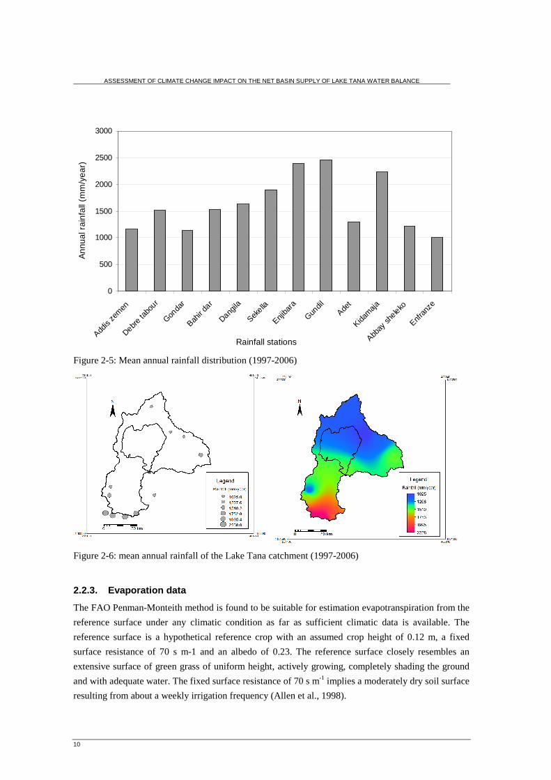
The mean annual rainfall map over the basin is calculated using the annual rainfall depth of the 12
stations (1997-2006) using inverse distance weighting interpolation in ILWIS and it shows that the
rainfall distribution is decreases from the south to the north. The mean annual rainfall of the basin is
1624 mm. The maximum annual average rainfall of 2467 mm is observed at Gundil station while the
minimum of 1140 mm at Gonder station.
ASSESSMENT OF CLIMATE CHANGE IMPACT ON THE NET BASIN SUPPLY OF LAKE TANA WATER BALANCE
10
0
500
1000
1500
2000
2500
3000
Addis
zem
en
Debre
tabo
ur
Gonda
r
Bahir
dar
Dangila
Sekella
Enjiba
ra
Gundil
Adet
Kidam
aja
Abbay
sheleko
Enfra
nze
Rainfall stations
Ann
ual r
ainf
all (
mm
/yea
r)
Figure 2-5: Mean annual rainfall distribution (1997-2006)
Figure 2-6: mean annual rainfall of the Lake Tana catchment (1997-2006)
2.2.3. Evaporation data
The FAO Penman-Monteith method is found to be suitable for estimation evapotranspiration from the
reference surface under any climatic condition as far as sufficient climatic data is available. The
reference surface is a hypothetical reference crop with an assumed crop height of 0.12 m, a fixed
surface resistance of 70 s m-1 and an albedo of 0.23. The reference surface closely resembles an
extensive surface of green grass of uniform height, actively growing, completely shading the ground
and with adequate water. The fixed surface resistance of 70 s m-1 implies a moderately dry soil surface
resulting from about a weekly irrigation frequency (Allen et al., 1998).

ASSESSMENT OF CLIMATE CHANGE IMPACT ON THE NET BASIN SUPPLY OF LAKE TANA WATER BALANCE
11
This method requires daily records of maximum temperature, minimum temperature, relative
humidity, wind speed and sunshine hours. Therefore Bahir Dar, Gonder, Debre Tabour and Dangila
stations are selected for this study because of availability of sufficient records from 1997-2006 for
estimation of evaporation.
Figure 2-7: mean annual Penman-Monteith reference evaporation of Lake Tana catchment (1997-
2006)
The mean annual reference evaporation map of the basin is made using the climate data of the above 4
stations from 1997-2006 using the inverse distance interpolation in ILWIS. The mean annual
reference evaporation is low in the southern and eastern part of the Lake Tana basin while the
reference evaporation is high in the northern part. The mean yearly reference evaporation within these
periods are 1356 mm, 1561 mm, 1265 mm and 1294 mm based on Bahir Dar, Gonder, Debre Tabour
and Dangila station respectively. The highest evaporation is estimated at Gonder station while the
lowest is estimated at Debre Tabour station.
The average monthly reference evaporation also indicates that the highest evaporation is observed at
Gonder stations while at Debre Tabour station the evaporation is low. Seasonally maximum reference
evaporation is observed in the March, April and May but in the wet season (June, July and August)
the evaporation has the lowest record.
Solar radiation is the main driving force for evaporation. High temperature results an increase of
evaporation while low temperature reduces the evaporation despite the wind speed, humidity and
other climate factors also have the impact. Topography of the catchment has an influence in the
evaporation. At higher elevation the temperature is higher than the lower elevation area. Therefore the
evaporation is maximum at high elevation than lower elevation area.

ASSESSMENT OF CLIMATE CHANGE IMPACT ON THE NET BASIN SUPPLY OF LAKE TANA WATER BALANCE
12
0
5
10
15
20
25
30
35
Jan-
97
Jul-9
7
Jan-
98
Jul-9
8
Jan-
99
Jul-9
9
Jan-
00
Jul-0
0
Jan-
01
Jul-0
1
Jan-
02
Jul-0
2
Jan-
03
Jul-0
3
Jan-
04
Jul-0
4
Jan-
05
Jul-0
5
Jan-
06
Jul-0
6
Time
Max
imum
Tem
pera
ture
( o C
)
Bahir DarGonderDangilaDebre Tabour
Figure 2-8: Monthly maximum temperature of four satations (1997-2006)
0
2
4
6
8
10
12
14
16
18
20
Jan-
97
Jul-9
7
Jan-
98
Jul-9
8
Jan-
99
Jul-9
9
Jan-
00
Jul-0
0
Jan-
01
Jul-0
1
Jan-
02
Jul-0
2
Jan-
03
Jul-0
3
Jan-
04
Jul-0
4
Jan-
05
Jul-0
5
Jan-
06
Jul-0
6
Time
Min
imum
tem
pera
ture
( o C
)
Bahir Dar GonderDangila Debre Tabour
Figure 2-9: Monthly minimum temperature of four stations (1997-2006)

ASSESSMENT OF CLIMATE CHANGE IMPACT ON THE NET BASIN SUPPLY OF LAKE TANA WATER BALANCE
13
60
70
80
90
100
110
120
130
140
150
160
Janu
ary
Feb
ruar
y
Mar
ch
Apr
il
May
June
July
Aug
est
Sep
tem
ber
Oct
ober
Nov
embe
r
Dec
embe
r
Month
evap
orat
ion
(mm
/mon
th)
Bahir DarGonderDebre TabourDangila
Figure 2-10: Monthly average reference evaporation (1997-2006)
In Lake Tana basin the highest maximum monthly temperature of 32 oC is observed in May 2003 at
Gonder station while the lowest monthly maximum temperature of 17 oC is observed in July 1999.
The mean monthly maximum temperature of 27.3 oC, 27.4 oC, 25.2 oC and 22.2 oC are observed at
Bahir Dar, Gonder, Dangila and Debre Tabour stations respectively. The trend indicates that the
highest monthly maximum temperature is observed in March, April and May and the lowest
maximum temperature is observed in the wet season of the year (June, July, August and September)
because of rainfall, cloudy condition and energy used for evapotranspiration.
The highest monthly minimum temperature of 18 oC is also observed at Gonder station in May 2003
while the lowest monthly minimum temperature of 3.4 oC is observed in January 2001 at Dangila
station. In March, April and May the minimum temperature shows an increasing trend while in the
month of December, January and February, which are part of the dry season, the minimum
temperature shows the lowest trend in the analysis period.

ASSESSMENT OF CLIMATE CHANGE IMPACT ON THE NET BASIN SUPPLY OF LAKE TANA WATER BALANCE
14

ASSESSMENT OF CLIMATE CHANGE IMPACT ON THE NET BASIN SUPPLY OF LAKE TANA WATER BALANCE
15
3. Literature review
3.1. Climate scenarios
A climate scenario is a reasonable prediction of the future climate change. There are different climate
scenarios used for climate change studies, among them synthetic scenario, analogue scenario and
scenario based on general circulation model output are the most widely used.
In a synthetic scenario the future temperature and the precipitation is changed by a realistic but
arbitrarily chosen value. It is most widely used for exploring system sensitivity prior to the application
of more credible, and model based scenario. Analogue scenario is based on identifying recorded
climate region which may have the same record of the future climate in a given region. But this
scenario has its own drawback for climate change assessment because it is difficult to get climate data
in the present which will have the similar record in the future. Scenarios from general circulation
model outputs is different from the others since it is a numerical model which represents physical
processes in the atmosphere, ocean and land surface by modelling the response of global climate
system to increasing green house gas concentrations (Carter, 2007).
For this study the model is selected based on the following criteria:
• The model should be consistent in global projection
• The model should be physically plausible
• The model should be easily available and
• The model should be representative
Most GCM outputs are able to simulate the global and continental climate processes in detail and
gives accurate climate prediction in the future (Dibike and Coulibaly, 2005). The GCM is a coarser
resolution and correctly model smoothly varying fields such as surface pressure and temperature but
unlikely these models properly simulate non smoothing fields such as precipitation (Mujumdar, 2008).
The scenario based on the GCM output is selected for this study since it has firm physical bases,
easily available and it is physically plausible.
3.2. General circulation model (GCM)
The Intergovernmental Panel on Climate Change (IPCC) data distribution centre (DDC) have seven
general circulation modelling centres for getting daily climate variable for climate change studies .
Each model has a unique approach to modelling these complex systems, differing in their levels of
resolution and degree of specificity. Very recent GCMs are coupled models that include four principal
components: atmosphere, ocean, and land surface and sea ice. The GCM uses the future forcing
scenarios to produce the range of the climate change. The selection of each model for a particular
climate change study depends on time of the model development, the resolution of the model, the
validity of the model, the representativeness of the model output and the availability of the model.

ASSESSMENT OF CLIMATE CHANGE IMPACT ON THE NET BASIN SUPPLY OF LAKE TANA WATER BALANCE
16
Table 3-1: Coupled atmospheric general circulation models for which climate change simulation held
by IPCC Data Distribution centre (Carter, 2007).
Modelling centre Country models
Common wealth scientific and industrial research
organisation(CSIRO)
Australia CSIRO-MK2
Max Planck Institute for Meteorology
Germany ECHAM4/OPYC and
EPHAM3/LSG
Hadley centre for climate prediction and research UK HadCM2&HadCM3
Canadian centre for climate modelling and
analysis (CCCMA)
Canada CGCM1&CGCM2
Geophysical fluid dynamic laboratory(GFDL) USA GFDL-R15&GFDL- R30
National centre for atmospheric research(NCAR) USA NCAR DOE-PCM
Centre for climate research studies (CCSR) and
national institute for environmental studies (NIES)
Japan CCSR-NIES
HadCM3 is a coupled atmospheric-ocean GCM developed at the Hadley Centre of the United
Kingdom National Meteorological Service that studies climate variability and change. The model
includes different land cover classification, soil layers and detail evapotranspiration function (Palmer
et. al., 2004).
The atmospheric component of the model has 19 levels with a horizontal resolution of 2.5o latitude
and 3.75o longitude. The ocean component of the model has 20 levels with horizontal resolution 1.25o
latitude and 1.25o longitude.
3.3. Emission scenarios
Emission scenarios are based on prediction of possible population growth, economic development and
the available energy utilization in the future world. Its major aim is to identify the future environment
related with the production of greenhouse gases. Based on the IPCC Special Report on the Emission
Scenarios (SRES) A1, A2, B1 and B2 are the four major emissions to indicate the future increase of
green house gases and aerosol concentration.
In A1 scenario the global population become 8.7 billion in the mid-century and reduced to 7 billion by
2100. A1 emission scenarios are further classified in to A1F1, A1T and A1B based on the alternative
energy requirement. In A2 emission scenario the population by 2100 become 15 billions and
technology become slower than other scenario. In B1 emission scenario the population growth is
almost similar to the A1 scenario but the technological change is more on the social service and
information. The population growth in B2 emission scenario less than A2 and the there is also

ASSESSMENT OF CLIMATE CHANGE IMPACT ON THE NET BASIN SUPPLY OF LAKE TANA WATER BALANCE
17
intermediate economic growth as compared to other emission scenarios. In addition to this the
scenario focuses on the environmental protection (Carter, 2007).
The IPCC recommends the use of A2 (high emission) and B2 (medium-low emission) for inter-
comparison studies because the computing cost of all the scenarios in GCM is too expensive. These
two scenarios are the only one that was common to all GCMs. The fact that the inter-model variability
higher than the inter-scenario variability also supports the choice of those two scenarios being
adequate (Menzel and Bürger, 2002).
3.4. Downscaling methods and tools
GCM were not designed for climate change impact studies and do not provide a direct estimation of
hydrological response to climate change. Therefore in climate change impact studies, hydrological
models are needed to simulate sub grid scale phenomena. However, such hydrological model requires
input data (such as precipitation) at similar sub grid scale, which has to be provided by converting the
GCM output into at least a reliable daily rainfall series at the selected watershed scale. The method
used to convert GCM output in to local meteorological variables required for reliable hydrological
modelling are usually referred to as ‘downscaling’ techniques (Dibike and Coulibaly, 2005).There are
two categories of climate downscaling namely dynamic downscaling and statistical downscaling.
They are described in the next sections.
3.4.1. Statistical downscaling
Statistical downscaling is used to relating the large scale atmospheric predictor variables to finer
resolution meteorological series which could be used as input to hydrological models (Dibike and
Coulibaly, 2005).
Statistical downscaling model requires the availability of long and homogeneous data series but the
computational resource needed are small. One of the basic advantages of the model is that they are
computationally inexpensive and it can easily apply to different GCM experiment (Wilby et al.,
2004). In SDSM the multiple linear relations developed between the predictors and the actual
meteorological data (predictand) for the current condition is applicable for future climate that exists
under different forcing conditions. The limitation of the SDSM is it requires long time series climate
data which may not be readily available in remote or complex topographic regions. The other
limitation of the model is that since it is empirical based method then it does not consider any
systematic change in the regional forcing conditions or feedback processes.
A diverse range of statistical downscaling techniques have been developed over the past few years
and each method lies in one of the three major categories namely, regression method, stochastic
weather generator and weather typing scheme.

ASSESSMENT OF CLIMATE CHANGE IMPACT ON THE NET BASIN SUPPLY OF LAKE TANA WATER BALANCE
18
I. Regression method
In regression downscaling methods the predicators (climate variables) and the predictand (actual data)
are correlated with multiple linear regression equation. As compared to other downscaling models the
regression method is easy for application and the model is freely available (Dibike and Coulibaly,
2005). In regression downscaling model there is limited correlation between the daily global climate
variables and the precipitation then the simulation capability of the model for precipitation is low
(Menzel and Bürger, 2002).
II. Stochastic Weather generator
Weather generators are models that replicate the statistical attributes of local climate variables (such
as mean and variance) but not the observed sequence of events. These models are based on
representation of precipitation occurrence on the Markov chain approach and spell length approach. In
Markov chain approach the random process is constructed which determine the day at station as rainy
or dry based on the previous day and following the given probability. When the day is wet the amount
is determined from the precipitation distribution of that particular month from the previous record or
the amount of precipitation on the previous days. In spell length approach instead of simulating
rainfall occurrence day by day, the models operates by fitting probability distribution to observed
relative frequencies of wet and dry spell length (Dibike and Coulibaly, 2005). In both cases the
statistical parameters (mean and variance) extracted from the observed data at a particular station
together with some random component are used to generate a similar time series of any length. In
stochastic weather generator the secondary variables such as wet day amount, temperature and solar
radiation are often modelled conditional on precipitation occurrence (Wilby et al., 2004).
III. Weather typing scheme
Weather typing scheme involves grouping local, meteorological data in relation to prevailing pattern
of atmospheric circulation. Climate change scenario are constructed either by re-sampling from the
observed data distribution (conditional on the circulation pattern produced by a GCM) or by
generating synthetic sequence of weather pattern and then re-sampling from the observed data. The
most serious limitation of the approach is that precipitation changes produced by changes in the
frequency of the weather patterns are seldom consistent with the changes produced by the host GCM
(Dowson & Wilby, 2007).
3.4.2. Dynamic downscaling
As it is discussed in the previous section the statistical downscaling model uses the coarser resolution
climate model (GCM) in order to get catchment scale climate variables, while the dynamic
downscaling uses a finer resolution of regional climate model (RCM) which has a horizontal
resolution of 20-50km. The SDSM is ultimately limited by the assumption of temporal stationary in
the empirical relations but dynamic downscaling model does not have such problems. Dynamic
downscaling simulations of local climate are more physically based than SDSM and are more

ASSESSMENT OF CLIMATE CHANGE IMPACT ON THE NET BASIN SUPPLY OF LAKE TANA WATER BALANCE
19
acceptably transferable from the current to the future climate. However, dynamic downscaling
simulation of the current climate has not been extensively tested (Hay and Clarck, 2003).
The main advantage of RCMs is that they can resolve small scale atmospheric features such as
orographic precipitation better than the GCM. Furthermore, RCMs can be used to explore the relative
significance of different external forcing such as terrestrial ecosystem or atmospheric chemistry
changes (Dowson & Wilby, 2007). Even though the RCM has the advantage over the GCM in
simulating finer resolution climate variables, there also have their own drawback. The basic drawback
of RCM is it requires considerable computing resources and it is expensive to run as the GCM (Abdo
Kedir, 2008).
3.5. Water balance models
Water balance models are classified as physically based, conceptual and empirical depending on the
degree of complexity and physical completeness in the formation of the structure. Models are further
classified as lumped, semi distributed and distributed depending on the degree of discretization when
describing the terrain in the basin. Today most rainfall runoff models, whether physically based or
conceptual are distributed to some degree and larger basins are regularly split into subbasins in model
application (Bergström and Graham, 1998).
Distributed model structure accounts for detailed catchment characteristics (e.g. soil and land use),
process calculation and highly resolved meteorological variables (e.g. precipitation). The catchment is
divided in to a number of subcatchments and each subcatchment is further divided in to a number of
grid cells. In the semi distributed model structure, sub division of subcatchment in to a number of
different homogeneous zones can be accomplished based on various catchment characteristics
(topographic elevation, soil type and land use). Whereas in fully lumped model, the meteorological
variables, precipitation, temperature and potential evaporation were assigned to each subcatchment
(Das et al., 2008).
Empirical models are based on the mathematical equations which do not take into account the
physical processes and therefore are not useful for implementation of the appropriate model
components. Physically based model on the other hand incorporate physical laws based on
conservation of mass, momentum and energy. In physically based model there is a problem of over
parameterization because different combination of parameters giving equally good performance.
Besides this over parameterization effect, physically based model generally incorporate too many
process and too complex formulation at a too detailed scale on the context of climate change.
Conceptual model usually able to capture the dominating hydrological process at the appropriate scale
with accompanying formulations. Therefore conceptual model is considered as a nice compromise
between the need for simplicity on one hand and the need for firm physical bases on the other hand
for climate change study (Booij, 2005).

ASSESSMENT OF CLIMATE CHANGE IMPACT ON THE NET BASIN SUPPLY OF LAKE TANA WATER BALANCE
20
Sacramento, MIKE-SHE, Topmodel and HBV model are some of the major rainfall runoff model used
for the continuous simulation of runoff. Sacramento model approach is a lumped conceptual model
used for the continuous stream flow simulation. The model accounts for effective rainfall, evaporation
and interception, storage of water in various zones and discharge from these zones and water transport
in the drainage system (Rientjes, 2007). Topmodel is classified as conceptual distributed and allows
for continuous stream flow simulation. The model domain is fully distributed and the approach is
mass conservative but applies relatively simple momentum type equivalency to simulate the stream
flow. In Topmodel approach, topography of a catchment is analysed by means of a digital elevation
model to represent the topography of the catchment in to a number of rectangular grid element.
MIKE-SHE is physical based distributed catchment modelling system that is developed from 1977
onwards by the Danish Hydraulic Institute (DHI), the Institute of Hydrology in the U.K. and the
French consulting company SOGREAH (Rientjes, 2007). The model process includes rainfall, canopy
interception, evapotranspiration, snow melt, overland flow, channel flow, unsaturated subsurface flow
and saturated subsurface flow.
HBV model is a semi distributed conceptual hydrological model for a continuous simulation of
runoff. In the model it is possible to forecast the runoff from the individual subcatchment and add the
contribution to get the total inflow from the catchment. When the subcatchment has a considerable
elevation difference it is divided in to different elevation zone and each elevation zones is further
divided in to forest and non forest (SMHI, 2006).
The dominating processes of the HBV model are precipitation, evapotranspiration, subsurface flow
and river flow. The different subcatchments and elevation zones are used to obtain appropriate spatial
scale and the simulation can be done with different time steps. The process of infiltration, saturation
excess overland flow and subsurface storm flow is represented by one component called the runoff
generation routine. The advantages of HBV model are (a) it covers most of the important runoff
generating process by quite simple and robust structures and does not requires too extensive input data
(b) it accounts for topographic conditions by defining elevations zones within the basin or subbasins
and (c) the model was successfully tested in different conditions in more than 40 countries
(Krysanova et al., 1999).
The other advantage of HBV model compared to other hydrological model for climate change study is
because of its availability and firm physical basis for simulating of runoff and its application covers
basins of different climataological and geographical regions ranging in size from less than 1 to more
than 40,000km2 area (Booij, 2005).

ASSESSMENT OF CLIMATE CHANGE IMPACT ON THE NET BASIN SUPPLY OF LAKE TANA WATER BALANCE
21
4. Methodology
4.1. Statistical analysis of observed data
To analyze the trends of observed maximum temperature, minimum temperature and rainfall data of
Bahir Dar, Gonder and Debre Markos station, statistical analyses are considered. For this study
significance testing using confidence intervals of least square is applied for analyzing the temperature
and rainfall change for the time period 1961-2007 for which daily observations are available. First a
simple linear regression model of ii bxay +=∧
is selected and then it is tested whether b is
significantly different from zero. In the linear model a is the constant value of temperature or rainfall
and b is the change per year (slope), ix is a year to which the output is calculated by the model and
iy∧
is the estimated rainfall or temperature by the linear model.
The variance is calculated by:
( )2
2
2−
+−=∑
N
bxay ii
σ [4-1]
Where 2σ = variance in (mm) 2 for rainfall and (oC) 2 for temperature.
iy = the observed time series data (mm for rainfall and oC for temperature)
ibxa + = the output of the linear model (mm for rainfall and oC for temperature).
N = sum of observation years from 1961 to 2007.
ix = the observed years from 1967 to 2007
From the above equation it can be shown that the regression coefficient b will have the student-t
distribution with variance.
[ ] ( )2
2
var∑ −
=xx
bi
σ [4-2]
Based on the variance of b, the t distribution table is used to define the multiplier t for the confidence
limits for the regression coefficient under the hypothesis of no climate change.

ASSESSMENT OF CLIMATE CHANGE IMPACT ON THE NET BASIN SUPPLY OF LAKE TANA WATER BALANCE
22
( )btb var±= β [4-3]
For t test analysis the slopeβ is equal to some specified value oβ (often assumed as 0). This is
because it has to be tested that there is climate change ( )0≠β and the hypothesis that there is no
climate change( )0=β . Therefore based on this it is possible to estimate the current climate change
with a specified confidence interval.
4.2. General circulation model
Among the different GCMs the HadCM3 model is selected for this study since the model is widely
used for climate change impact assessment. Besides this the model is selected due to the availability
of the downscaling models called SDSM that is used to downscale the result of HadCM3. For
HadCM3 the model result is available for A2 and B2 emission scenario, where A2 is refereed to as
medium-high emission scenario and B2 is medium-low emission scenario. For both scenarios the
ensemble members a, b, and c are available which refer to a different initial point of climate solution
along the reference period (Hanson et al, 2004). But for this study the data is available for the “a”
ensembles and hence only the A2a and B2a scenarios are considered.
4.3. Statistical downscaling model (SDSM)
The selected regression based method is the SDSM 4.2 developed by Dowson and Wilbey (2007) and
it is downloaded freely from http://www.sdsm.org.uk. It is a decision support tool used to assess local
climate change impacts using a statistical downscaling technique. The tool facilitates the rapid
development of multiple, low cost, single site scenarios of daily surface weather variables under
current and future climate forcing. The model is calibrated and applied at a daily time series even
though the output is at monthly basis.
The software manages additional tasks of data quality control and transformation, predicator variable
screening, automatic model calibration, statistical analysis and graphing of climate data.
4.3.1. Downloading the predictors
General circulation model (GCM) predictors are freely obtained from the Canadian Climate Impact
Scenario Group with web address of: http://www.cics.uvic.ca/scenarios/sdsm/select.cgi/.
The predictor variables of HadCM3 are available on a grid box by grid box basis of size 2.5o latitude
and 3.75o longitude. The Lake Tana basin found between 36o 43’ 59” E to 38o 14’ 32”E (average
37.488o E) and 10o56’45”N to 12o45’22”N (average 11.851oN). Hence the nearest grid box which
represents the study area to download the HadCM3 data is 12.5oN and 37.5oE (see Figure 4-1). The
NCEP_1961-2001 data is downloaded from the specified grid box which represents the Lake Tana

ASSESSMENT OF CLIMATE CHANGE IMPACT ON THE NET BASIN SUPPLY OF LAKE TANA WATER BALANCE
23
basins. This data is used for calibration of the SDSM with the actual maximum temperature, minimum
temperature and precipitation.
Figure 4-1: Downloading site of Climate variable
Table 4-1: Predictor variables of the climate scenarios (Dawson & Wilby, 2007)
No
Predictor
variables predictor description No
Predictor
variables predictor description
1 mslpaf mean sea level pressure 14 p5zhaf 500hpa divergence
2 p_faf surface air flow strength 15 p8_faf 850hpa air flow strength
3 p_uaf surface zonal velocity 16 p8_uaf 850 hpa zonal velocity
4 p_vaf Surface merdional velocity 17 p8_vaf 850 hpa meridional velocity
5 p_zaf surface vorticity 18 p8_zaf 850 hpa vorticity
6 P_thaf surface wind direction 19 p850af 850 hpa geopotential
7 p_zhaf surface divergent 20 p8thaf 850 hpa wind direction
8 p5_faf 500hpa airflow strength 21 p8zhaf 850hpa divergence
9 p5_uaf 500hpa zonal velocity 22 pr500af Relative humidity at 500hpa
10 p5_vaf 500hpa merdional velocity 23 pr850af Relative humidity at 850hpa
11 p5_zaf 500hpa vorticity 24 rhumaf Near surface relative humidity
12 p500af 500hpa geopotential height 25 shumaf Surface specific humidity
13 p5thaf 500hpa wind direction 26 tempaf Mean temperature at 2 metre
4.3.2. Preparation of predictands
Maximum temperature, minimum temperature and rainfall records from 1961-1990 of Bahir Dar,
Gonder and Debre Markos have been prepared for inputs to the statistical downscaling model. In the
time series data there are some outliers, missing data and gap data that should be corrected before it
can be used in the model. The outliers are the values that highly deviate from the mean value. The
missing data and gap data are less than 1% of the total data available from the meteorological and
hydrological stations. In order to fill data the correlation is done with the individual station which has
the missing and gap data and the average of the nearby stations which do not have such problem. Then

ASSESSMENT OF CLIMATE CHANGE IMPACT ON THE NET BASIN SUPPLY OF LAKE TANA WATER BALANCE
24
based on the regression equation the missing and the gap data of the individual station is filled with
respect of the available data of the other stations.
4.3.3. Model parameters
In the SDSM before doing any analysis the first step is fixing the model parameters which are basic to
the temperature and precipitation simulation. Maximum temperature and minimum temperature are
continuous processes while rainfall occurs in events. Therefore to treat less rain days as dry days an
event threshold of 0.1 mm/day is used for precipitation while no event threshold is required for
temperature. A statistical method is more straightforward than dynamic downscaling but tends to
underestimate variance and poorly represent extreme events. Regression method under predict climate
variability to varying degrees, since only parts of the regional and local climate variability is related to
large scale climate variations . The range of variation of the downscaled and daily weather parameters
can be controlled by fixing the variance inflation. This parameter changes the variance by adding
/subtracting equal amount applied to regression model estimates of the local process. Then variance
inflation of 12 prior to any model transformation produces normal variance inflation for daily
temperature values, while for daily precipitation the variance inflation of 18 is added to agree with the
observed climate variables.
The choice of statistical method is to some extent determined by the nature of the local predictand. A
local variable that is reasonably normally distributed, such as temperature will require nothing more
complicated than multiple regression, since the large scale climate predictors are normally distributed
and assuming linearity of the relationship. A local variable that is highly heterogeneous and
discontinuous in space and time, such as daily precipitation, will require a more complicated non-
linear approach or transformation of raw data to be consistent with the large scale predicator variable.
Therefore the fourth root transformation is applied to the raw data of the precipitation prior to model
calibration.
4.3.4. Screening downscaled predicator variables
Screening is identifying the downscaled predicators which have high correlation with the actual
climate variable. The method correlates each predictands (observed maximum and minimum
temperature and rainfall) of Bahir Dar, Gonder and Debre Markos with the 26 NCEP downloaded
predictors data. The strength of the individual predictors varies on a month by month basis. Therefore
most appropriate combination of predictors has to be chosen by looking at the analysis output of the
twelve months. The predicators which have significant correlation with each predictands and low
correlation with the individual predictors should be selected for calibration.
4.3.5. Model calibration
The calibration of the statistical downscaling model is based on the multiple linear regressions
between the screened predictors and the predictand. Twelve multiple linear regression equations for
each months are produced automatically between the predictand and the screened predictors. For

ASSESSMENT OF CLIMATE CHANGE IMPACT ON THE NET BASIN SUPPLY OF LAKE TANA WATER BALANCE
25
model calibration the predictands of daily maximum temperature, minimum temperature and rainfall
of the Bahir Dar, Debre Markos and Gonder stations are used. The calibration is done based on the 30
year actual data from 1961-1990 since this period is the baseline period for most climate change
impact assessment.
In calibration of the SDSM the process type that identifies the presence of the intermediate process in
the predictor-predictand relationship must be defined. In unconditional process there is the direct link
between the predicator and the predictand (e.g., maximum and minimum temperature are directly
depends on mean temperature at 2 metre height). In conditional process, there is an intermediate
process between the predicators and the predictand (e.g., precipitation amount depends on the
occurrence of wet day, which in turn depends on predicators of relative humidity).
In unconditional process the predictand and predictors are correlated with automatic calibration
method without any intermediate process. But in conditional process like precipitation first the daily
probability of non-zero precipitation (a wet day) for a given day is determined with autocorrelation
before calibrating the precipitation amount. If the precipitation has occurred the daily precipitation
amount is calculated based on the selected screened predictors. Therefore unconditional process is
used for maximum and minimum temperature while the conditional process is used for precipitation.
After calibrating the model for each station with the actual data the next step is checking whether the
model is able to reproduce the actual data or not. This is done with two methods the first is visual
inspection of the modelled value and the actual value from 1961-1990 and the other is by checking the
absolute model error and variance of the modelled and the observed data.
4.3.6. Scenario generation
For scenario generation H3A2a-1961-2099 and H3B2a_1961-2099 are downloaded from the same
web site as the NCEP data (see section 4.3.1). The predictors are the same type as the NCEP
predictors, the difference is that the NCEP predictors used for model calibration while the H3A2a and
H3B2a are used for scenario generation. The regression weights produced during the calibration
process were applied to the time series outputs of the GCM model. This is based on the assumption
that the predictor-predictand relationships under the current condition remain valid under future
climate conditions too.
Twenty ensembles of synthetic daily time series data were produced for two of the SERS scenarios for
the above future time horizons in order to increase the performance of the model. The final product of
the SDSM downscaling method was then found by averaging the twenty independent GCM
ensembles. The differences between the 20 ensembles do not reflect the full range of internal
variability because only the stochastic component differs in each run. The deterministic component
(i.e. controlled by the atmospheric circulation and moisture variables) follows the same evolution in
each run because only one source of predictor (i.e. either the NCEP or HadCM3 ) variables exists in
each case (Goodess et al., 2003).

ASSESSMENT OF CLIMATE CHANGE IMPACT ON THE NET BASIN SUPPLY OF LAKE TANA WATER BALANCE
26
The scenario is generated for three future time horizons, from 2011-2039, 2040-2069 and 2070-2099
and for the baseline period 1961-1990 based on HadCM3A2a and HadCM3B2a.
Table 4-2: Scenario periods
Run Start date End date
1st run 1961 1990
2nd run 2010 2039
3ndrun 2040 2069
4th run 2070 2099
Once the scenario data is computed in the future period, the monthly change of temperature and
rainfall from the baseline period for Bahir Dar, Gonder and Debre Markos stations is calculated.
These changes in temperature and relative change in precipitation are superimposed up on 30 years
climate records and used as input for hydrological model. The change observed in one month is added
to every day record of the same months in the 30 years climate data. The 30 years climate data are the
actual data of maximum temperature, minimum temperature and rainfall of the above three station
used for statistical downscaling model.
4.4. Lake evaporation
Open water evaporation is important for computation of the net basin supply of Lake Tana water
balance from 2010-2099 in future time period and from 1961-1990 in baseline period. Open water
evaporation can be calculated with modified Penman method based on the observation of wind speed,
sunshine hours and relative humidity and temperature. But only the 1997-2006 climate data are
available from the meteorological office required for Penman evaporation estimation. Therefore to
estimate the lake evaporation in the future time periods temperature index methods are required of
which the Hargreaves is best known method. The Hargreaves method is as follows:
( ) ( ) ameanO RTTTET 8.170023.0 5.0minmax +−= [4-4]
Where all temperatures are in oC and ET is evaporation in mm/day. The mean temperature is
calculated as 0.5(Tmax+Tmin). Ra is the extraterrestrial short wave radiation in mm/day.
In order to check the accuracy of the Hargreaves method for open water evaporation estimation other
methods are considered and the result is compared with the Hargreaves method with 1997-200 climate
data. The Penman combination equation of (Maidment, 1993) is one of the methods for estimation of
lake evaporation provided that sufficient climatic data available. The Penman combination equation is
as follow:

ASSESSMENT OF CLIMATE CHANGE IMPACT ON THE NET BASIN SUPPLY OF LAKE TANA WATER BALANCE
27
( ) ( )λγ
γγ
DUARE hnp
*536.01*43.6** 2+
+∆++
+∆∆= [4-5]
Where: pE is potential evaporation from the lake surface (mm/day), nR is the net radiation exchange
for the free water surface (mm/day), hA is energy advected to the water body (mm/day), 2U is the
wind speed measured at 2 m (m s-1), D is the average vapour pressure deficit (kPa), λ is the latent
heat of vaporization (MJ kg-1 ), γ is psychometric constant (kPa oC-1) and ∆ is the slop of saturation
vapour pressure curve (kPa oC-1).
The mean annual lake evaporation based on this method is 2084.9 mm. It is over estimated compared
to the lake evaporation obtained from different studies at the same area (see Table 5-9). The reason is
that Maidment (1993) modify the original Penman equation for small open water bodies and it over
estimate for large lake like Lake Tana.
The modified Penman combination of (Vallet-Coulomb et al., 2001) is also tested for Lake Tana
evaporation estimation. The equation is described below:
γγ
γ +∆+
+∆∆= EaRE n [4-6]
Where E is the daily evaporation rate (mm day-1), the net radiation nR expressed as equivalent
evaporation rate (mm day-1), ∆ is the slope of the saturated vapour pressure curve at the air
temperature, γ is the psychometric constant , and Ea is the drying power of the air given as a daily
rate (mm day-1) by:
( )( )eeUEa w −−= 254.0126.0 [4-7]
Where 2U is the wind speed measurement at two metre high (m s-1), ( )eew − is the saturation deficit,
difference between the saturated (we ) and the actual (e ) vapour pressure (kPa).
Both methods are the same except that the weight of wind function for estimation of the evaporation
with (Maidman, 1993) is larger than the (Vallet-Coulomb et al., 2001). The mean annual lake
evaporation based on this method is 1729 mm. The method estimates of the Lake Tana evaporation
compared to the above method. The mean yearly lake evaporation with Hargreaves method is 1708
mm. Then it is possible to conclude that the Hargreaves method also gives good result for Lake Tana
evaporation. (Gieske et al., 2008) also indicates that the Hargreaves method which is based on the
temperature measurement of Gonder and Bahir Dar station provide good approximate values for open
water evaporation of Lake Tana.
The lake energy balance method is one the best method for inferring lake evaporation (Vallet-Coulmb
et al, 2001). The method does not require wind speed data. The general expression for energy balance
is:

ASSESSMENT OF CLIMATE CHANGE IMPACT ON THE NET BASIN SUPPLY OF LAKE TANA WATER BALANCE
28
SEHRn ∆++= λ [4-8]
Where Rn is the net radiation, Eλ is the latent heat flux (λ the latent heat of vaporization in J kg-1,
and E the evaporation rate in kg s-1 m-2), H the sensible heat flux, and S∆ the change of energy
storage in the lake (all terms expressed in W m-2). The net radiation (Rn ) results from the balance
short wave and long wave radiation:
( ) 11 RRRn s −−= α [4-9]
Where Rs the net short is wave radiation, 1R is net long wave radiation (W m-2) and α is the surface
albedo. In the absence of direct radiation measurement, daily short wave radiation can be calculated
with the Angstrom formula, which relates solar radiation to the extraterrestrial radiation and relative
sunshine duration. The Angstrom formula is as follow:
asss RN
nbaR
+= [4-10]
Where aR is the solar radiation at the top of the atmosphere (Wm-2), n is the actual sunshine hours
(hours), N is the maximum possible sunshine hours (hours), sa and sb are the regression constants.
Where no actual solar radiation data are available and no calibration has been carried out to improve
sa and sb parameters, the values sa = 0.25 and sb = 0.50 are usually recommended.
Lake Tana is the shallow lake and there is weak seasonal variation in temperature therefore change in
storage ( S∆ ) coulde be neglected. Therefore the equation 4-8 can be can be simplified by introducing
bown ratio (β ) to the general energy balance equation.
( )1+−
=βλ
GRE n [4-11]
( )[ ]
12
1212
ee
zzTT
E
H
−−Γ+−
== γλ
β [4-12]
Where 1T [K] and 1e [mbar] are air temperature and vapour pressure at height 1z [m] and 2T [K] and
2e [mbar] are the temperature and vapour pressure at height 2z [m], γ is the psychometric constant
[mbar K-1] and Γ is adiabatic lapse rate, generally taken as 0.0065Km-1. Γ can be neglected if the
distance between the Bown ratio measurement heights is less than 2m. So the final equation for the
bown ration from field measurement is:
[ ]12
12
ee
TT
E
H
−−
== γλ
β [4-13]
Since I do not have sufficient water surface temperature data of the Lake Tana it is difficult to
calculate the evaporation with the energy balance method. But the annual Lake evaporation estimated

ASSESSMENT OF CLIMATE CHANGE IMPACT ON THE NET BASIN SUPPLY OF LAKE TANA WATER BALANCE
29
by Alebachw (2009) by energy balance method considering different albedo for each month is
1818.08mm/ year. This result also comparable to the lake evaporation estimated by the Hargreaves
method earlier.
Therefore the evaporation from 2010-2039, 2040-2069 and 2070-2099 is calculated using Hargreaves
by the downscaled maximum and minimum temperature for Bahir Dar and Gonder station while the
1961-1990 evaporation is calculated by the observed data. The weight of each station for lake
evaporation is computed by inverse distance weighting method. Bahir Dar has a weight of 0.60 and
Gonder has a weight of 0.4 for the estimation lake evaporation. Then the lake evaporation is
calculated by multiplying the evaporation of each station with the weight calculated by inverse
distance interpolation method.
Figure 4-2: Methodology of statistical downscaling model

ASSESSMENT OF CLIMATE CHANGE IMPACT ON THE NET BASIN SUPPLY OF LAKE TANA WATER BALANCE
30
4.5. HBV model
4.5.1. HBV model structure
Among different hydrological models HBV-96 model is selected since it is applicable for climate
change impact assessment. The model is semi distributed conceptual hydrological model which
simulates runoff based on daily precipitation, daily mean temperature and a long term monthly
potential evapotranspiration.
Figure 4-3: Schematic representation of HBV-96 model (Seibert, 2002)
The Lake Tana basin is divided into 10 major subbasins and each subbasin is further divided in
different elevation zones in order to consider the effect of elevation on temperature and rainfall
estimation. The HBV model have precipitation and snow routine, the soil moisture accounting
routine, the runoff generation routines and the transformation function.
Actual evapotranspiration (EA) was computed as a function of soil moisture condition and potential
evapotranspiration (EP). When the soil moisture exceeded the storage threshold (LP), water would
evaporate at the potential rate. At the lower soil moisture value a linear relationship between the ratio
EP/EA and the soil moisture was used. The general storage variable (S) was formed by soil moisture
storage (SM) and the storage in the upper and lower response boxes respectively, (hUZ and hLZ).
Recharge to ground water was calculated through a non linear relationship between the ratio R/P and

ASSESSMENT OF CLIMATE CHANGE IMPACT ON THE NET BASIN SUPPLY OF LAKE TANA WATER BALANCE
31
the soil moisture. The runoff generation routine of the catchment was described by the outflow from
the upper non linear reservoir (QUZ) while the base flow (QLZ) was governed from the lower response
box which is filled by the percolation from the upper response box. Runoff from the catchment (Q)
was given by the sum of the outflow from the two response boxes.
4.5.2. HBV model inputs
The inputs for HBV model consists of daily rainfall, temperature, estimates of potential
evapotranspiration and catchment characteristics of the area.
I. Areal rainfall
12 stations in and around the Lake Tana basin (see Figure 2-3) are selected for the computation of the
areal rainfall for the each subbasins. The areal rainfall is computed by multiplying rainfall in each
station by a weight which is computed by inverse distance weighting. This method was chosen
because it takes in to account the rainfall distribution of every rainfall station. The rainfall stations
nearer to the interpolated point have the greater weight than the stations farther apart. The inverse
distance weighting method is given byequation [4-14].
∑
∑
=
=
∗=
n
im
i
n
ism
i
d
PdP
1
1
1
1
[4-14]
Where:
p = estimated areal average rainfall
Ps= rainfall at the station
di= distance of the station from the region centre
m= distance weight
n= number of meteorological stations.
II. Catchment data
The HBV model is a semi distributed model. Therefore a digital elevation map of the area was
prepared from SRTM with the resolution of 90 m for the delineation of the lake catchment. The
catchment area and the drainage network of the catchment are extracted with the DEM hydro
processing tool in the Integrated Land and Water Information System (ILWIS) software. The
catchment area is divided in to 10 major subcatchments and it is further divided in to different
elevation zones of 100 metre interval. Among the subcatchments Gilgel Abbay, Ribb, Gumra, Garno,
Gumero, Megech and Gelda are partly gauged while Gabi Kura, Derma and Tana West are unguaged
catchments. The unguaged catchments contribute 40 % of the total area of the catchment and the rest
is covered by gauged catchments. The Gilgel Abbay catchment includes the main Gilgel Abbay and a
number of tributaries such as Koga and Kelti. The Koga confluences with the Gilgel Abbay
downstream of Merawi and the Kelti confluences further downstream.

ASSESSMENT OF CLIMATE CHANGE IMPACT ON THE NET BASIN SUPPLY OF LAKE TANA WATER BALANCE
32
Projection: UTM, Datum: Adinidan, Ellipsoid: Clarke 1880
Figure 4-4: Major subcatchments of Lake Tana basin
Table 4-3: Catchment area of Lake Tana basin
Sub catchment Gauging location Gauged
area (km2 )
Unguaged
area (km2)
Total area of the
catchment (km2)
Gilgel Abbay Near Merawi 2562.7 1991 4553.7
Gumara Near Bahirdar 1280.6 517.3 1797.9
Ribb Near Addis Zemen 1301.8 711.5 2013.3
Megech Near Azezo 513.3 462.3 975.6
Garno Near Enfranze 97.4 256.5 353.9
Gemero Near Maksegnit 165.1 389.9 555
Gelda Near Ambesame 27 356.1 383.1
Tana West Unguaged 610.6 610.6
Gabi Kura Unguaged 382.5 382.5
Derma Unguaged 376 376

ASSESSMENT OF CLIMATE CHANGE IMPACT ON THE NET BASIN SUPPLY OF LAKE TANA WATER BALANCE
33
III. Evapotranspiration
The model uses monthly potential evapotranspiration as input. Therefore the data of Bahir Dar,
Gonder, Debre Tabour and Dangila are selected for estimation of evapotranspiration due to the
availability of sufficient climatic data. The FAO Penman-Monteith method is applied for estimation of
reference evapotranspiration since sufficient climate data are available from the above stations. The
weighted evapotranspiration in each basin is estimated by multiplying the evapotranspiration with the
weight of the station computed by inverse distance weighting.
( ) ( )( )2
2
34.01273
900408.0
u
eeuT
GRET
asn
O ++∆
−+
+−∆=
γ
γ [4-15]
Where:
OET = reference evapotranspiration [mm day-1]
nR = net radiation [MJ m-2 day-1]
G = soil heat flux [MJ m-2 day-1]
T = mean air temperature [oC]
2u = wind speed at 2 metre height [ms-1]
ae = actual vapour pressure [kpa]
se = saturation vapour pressure [kpa]
as ee − = saturation vapour pressure deficit [kpa]
∆ = slope vapour pressure curve [kpaoC-1]
γ = psychometric constant [kpaoC-1]
Table 4-4: Monthly reference evapotranspiration (mm/month)
Moths Bahir Dar Gonder Debre Tabour Dangila
January 101.3 114.0 106.7 103.5
February 113.0 123.2 114.2 113.4
March 136.2 144.0 130.0 133.8
April 140.5 147.0 121.0 137.3
May 136.1 142.6 119.9 131.5
June 112.5 107.8 88.9 94.2
July 92.9 85.7 79.2 84.9
August 92.3 87.7 84.5 84.3
September 102.9 105.5 89.5 94.3
October 114.2 116.6 96.4 92.6
November 105.7 105.0 94.9 93.0
December 102.4 105.4 104.4 96.3

ASSESSMENT OF CLIMATE CHANGE IMPACT ON THE NET BASIN SUPPLY OF LAKE TANA WATER BALANCE
34
IV. Land cover data
The land cover is further reclassified for each elevation zone according to the type required by the
HBV model. The HBV model requires forest, non forest, glaciers and lake. But in this study only
forest and non forest are considered because the glacier and the water bodies are almost negligible in
the elevation zones of the subcatchments. Based on the land cover data and the Penman-Monteith
reference evaporation, the HBV model calculates the potential evaporation of the catchment. The
actual evaporation is then calculated based on the potential evapotranspiration, the parameter called
limit of potential evaporation and the moisture content of the soil.
4.5.3. Objective function
The goodness of fit of the model to the observed discharge is estimated by two methods, relative
volume error and Nash-Sutcliffe coefficient which are represented by equation [4.10] and [4.11]
respectively.
The relative volume error of 0 indicates as there is no change between the observed and simulated
discharge. But it is difficult to conclude the performance of the model by estimating relative volume
error only because there may be a small value of relative volume error with wrong distribution of the
observed and simulated discharge. Therefore another performance indicator is essential together with
the relative volume error in order to accurately determine the model performance. The relative error
less than +5 % or -5% indicates that the model performs well and a relative volume error between +5
% to +10 % and -5 % to -10 % indicates the model is within reasonable performance.
1001 ×−
=∑
∑∑=
n
iobs
n
iobs
n
isim
Q
QQRVE [4-16]
Where: RVE = relative volume error, simQ = simulated flow and obsQ = observed flow
Nash-Sutcliffe coefficient is the other performance indicator used to assess the predictive power of the
hydrological model.
( ) ( )
( )∑∑ ∑
−
−−−=
2
22
2
obsobs
obssimobsobs
QQQQR [4-17]
Where: R2= Nash-Sutcliffe coefficient obsQ = the observed discharge, obsQ = mean of observed
discharge and simQ is the simulated discharge.
The perfect model would result in an R2 equal to 1. However, normally R2 ends up somewhere
between 0.8 and 0.95, this is only the case when good quality input data is available (SMHI, 2006).
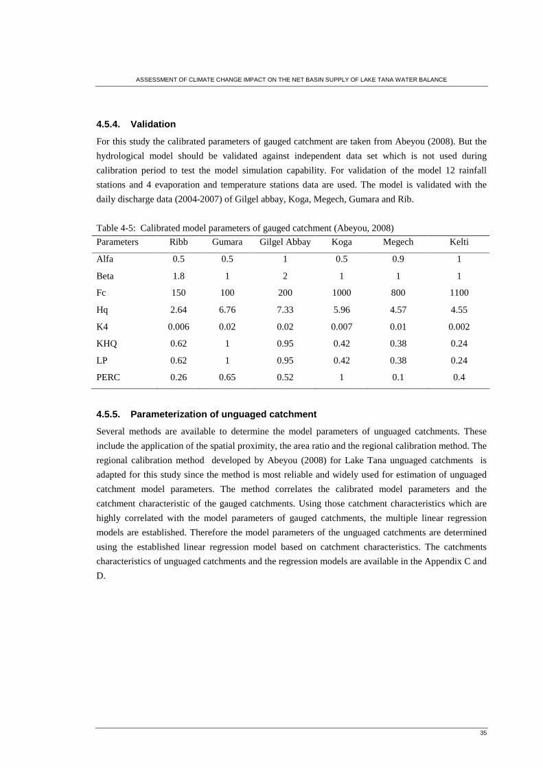
ASSESSMENT OF CLIMATE CHANGE IMPACT ON THE NET BASIN SUPPLY OF LAKE TANA WATER BALANCE
35
4.5.4. Validation
For this study the calibrated parameters of gauged catchment are taken from Abeyou (2008). But the
hydrological model should be validated against independent data set which is not used during
calibration period to test the model simulation capability. For validation of the model 12 rainfall
stations and 4 evaporation and temperature stations data are used. The model is validated with the
daily discharge data (2004-2007) of Gilgel abbay, Koga, Megech, Gumara and Rib.
Table 4-5: Calibrated model parameters of gauged catchment (Abeyou, 2008)
Parameters Ribb Gumara Gilgel Abbay Koga Megech Kelti
Alfa 0.5 0.5 1 0.5 0.9 1
Beta 1.8 1 2 1 1 1
Fc 150 100 200 1000 800 1100
Hq 2.64 6.76 7.33 5.96 4.57 4.55
K4 0.006 0.02 0.02 0.007 0.01 0.002
KHQ 0.62 1 0.95 0.42 0.38 0.24
LP 0.62 1 0.95 0.42 0.38 0.24
PERC 0.26 0.65 0.52 1 0.1 0.4
4.5.5. Parameterization of unguaged catchment
Several methods are available to determine the model parameters of unguaged catchments. These
include the application of the spatial proximity, the area ratio and the regional calibration method. The
regional calibration method developed by Abeyou (2008) for Lake Tana unguaged catchments is
adapted for this study since the method is most reliable and widely used for estimation of unguaged
catchment model parameters. The method correlates the calibrated model parameters and the
catchment characteristic of the gauged catchments. Using those catchment characteristics which are
highly correlated with the model parameters of gauged catchments, the multiple linear regression
models are established. Therefore the model parameters of the unguaged catchments are determined
using the established linear regression model based on catchment characteristics. The catchments
characteristics of unguaged catchments and the regression models are available in the Appendix C and
D.

ASSESSMENT OF CLIMATE CHANGE IMPACT ON THE NET BASIN SUPPLY OF LAKE TANA WATER BALANCE
36
Table 4-6: Model parameters of Unguaged catchments (after Abeyou, 2008)
catchment Alfa Beta FC Hq K4 KHQ LP PERC
Unguaged Gilgel Abbay 1.29 2.60 432 8.21 0.013 0.076 1.00 0.550
Unguaged Megech 1.00 1.27 1408 4.98 0.004 0.103 0.32 0.234
Unguaged Ribb 0.74 1.36 1101 3.80 0.025 0.093 0.27 0.086
Unguaged Gumara 1.00 1.28 1401 4.32 0.004 0.126 0.29 0.414
Gumero 0.83 1.18 1163 2.03 0.018 0.102 0.20 0.157
Garno 0.86 0.89 1143 2.98 0.07 0.100 0.16 0.06
Gelda 0.9 1.00 800 3.00 0.01 0.100 0.38 0.100
Derma 0.98 1.10 1381 2.20 0.02 0.103 0.13 0.120
Gabikura 1.11 1.26 1572 3.02 0.003 0.106 0.166 0.16
Tana West 0.63 1.14 977 3.49 0.037 0.114 0.317 0.344
4.6. Net basin supply of Lake Tana water balance
The net basin supply (N) is the major part of the Lake Tana water balance and it is estimated by the
lake precipitation, lake evaporation and the inflow to the lake (see equation 4.12).
o
in
A
QEPN +−= [4-18]
Where:
P = precipitation of the Lake Tana (mm/day)
E = evaporation of the Lake Tana (mm/day)
inQ = the inflow to Lake Tana (m3/s)
oA = surface area of the lake (km2)
No lake outflow data is used for the computation of the net basin supply because it is estimated only
by the lake precipitation; lake evaporation and the inflow to the lake. The unit of inflow component
should be consistent with the precipitation and the evaporation. Therefore the inflow to the lake is
multiplied by the factor 86.4 to convert m3/s to mm/day.
The net basin supply is calculated for the baseline period (1961-1990) and three future periods each
covering non overlapping 30 years. These periods are 2010-2039, 2040-2069 and 2070-2099. The
calibrated and validated HBV model is used for forecasting the inflow to the lake. The inputs of the
model are the downscaled maximum temperature, minimum temperature and precipitation. The
evaporation used for the model is also calculated from the downscaled temperature. The total inflow
to the lake is the sum of the inflows from each subcatchment. The inflow from each subcatchment is
computed based on the Bahir Dar, Gonder and Debre Markos precipitation, temperature and

ASSESSMENT OF CLIMATE CHANGE IMPACT ON THE NET BASIN SUPPLY OF LAKE TANA WATER BALANCE
37
evapotranspiration. The weight of each station to the catchment is calculated by the inverse distance
weighting method. The lake evaporation and lake precipitation is calculated by the Bahir Dar and
Gonder climatic data as well.
It is very essential to estimate the lake surface area for computation of the net inflow to the lake. To
estimate the lake area it is necessary to analyse the changes with respect to volume of the lake and
elevation of the lake. For this purpose the bathymetric survey done by Kaba Ayana (2007) is
considered to get the relation of the lake surface area and lake elevation with the volume of the lake.
The Bathymetry done by Kaba Ayana (2007) is further developed by Abeyou (2008) by increasing
additional data set in the lake not covered by Kaba Ayana (2007) to increase the accuracy of the
interpolation. The interpolation result of bathymetric survey is as follow:
Polynomial fitted bathymetry by Abeyou (2008)
63.177410*2.610*02.110*21.1 428313 ++−= −−− VVVE [4-19]
51.114710*65.110*81.510*93.7 126311 ++−= −−− VVVA [4-20]
1000
1500
2000
2500
3000
3500
0 5000 10000 15000 20000 25000 29060 35000
Volume (Mm3)
Are
a(km
2 )
1765
1770
1775
1780
1785
1790
1795
Ele
vatio
n (m
am
sl)
Abeyou (2008) A-V Abeyou (2008) E-V
Figure 4-5: Elevation-volume and area-volume relation of Lake Tana
Based on the Elevation-volume and area-volume relationship the elevation-area relation of the Lake
Tana is derived which is very essential to know the relation of the lake area with change in depth.

ASSESSMENT OF CLIMATE CHANGE IMPACT ON THE NET BASIN SUPPLY OF LAKE TANA WATER BALANCE
38
y = 0.568x3 - 3043.2x2 + 5E+06x - 3E+09
R2 = 0.99
1000
1500
2000
2500
3000
3500
1772 1774 1776 1778 1780 1782 1784 1786 1788 1790
Elevation m amsl
Are
a (k
m2 )
Abeyou (2008)
Poly. (Abeyou (2008))
Figure 4-6: Elevation-area ratio of Lake Tana
The elevation-area relation indicates that the surface area of the lake in general is increased by 145
km2 with 1 m increase in depth which is negligible compared to the total area of the lake. Therefore it
is reasonable to take a constant area of 3060 km2 for the computation of the net basin supply of Lake
Tana water balance. (Kebede et al., 2006) also consider constant surface area of Lake Tana for the
computation of the net basin supply since the change of lake surface area with change in depth is not
significant for the net basin supply computation.
Figure 4-7: Station used for downscaling of the climate variables

ASSESSMENT OF CLIMATE CHANGE IMPACT ON THE NET BASIN SUPPLY OF LAKE TANA WATER BALANCE
39
Table 4-7: Weight of precipitation, temperature and evaporation stations using inverse distance
weighting for net basin supply computation
Catchments Bahir Dar Gonder Debre Markos Catchments Bahir Dar Gonder
Gilgel Abbay 0.22 0.78 Unguaged Ribb 0.53 0.47
Koga 0.9 0.1 Unguaged Megech 0.03 0.97
Kelti 0.82 0.18 Gelda 0.96 0.04
Gumara 0.76 0.24 Garno 0.25 0.75
Ribb 0.59 0.41 Gemero 0.06 0.94
Megech 0.02 0.98 Tana West 0.53 0.47
Unguaged
Gilgel Abbay 0.93 0.07 Gabi Kura 0.15 0.85
Unguaged
Gumara 0.82 0.18 Derma 0.1 0.9
Figure 4-8: Methodology on the net basin supply computation

ASSESSMENT OF CLIMATE CHANGE IMPACT ON THE NET BASIN SUPPLY OF LAKE TANA WATER BALANCE
40

ASSESSMENT OF CLIMATE CHANGE IMPACT ON THE NET BASIN SUPPLY OF LAKE TANA WATER BALANCE
41
5. Result and discussion
5.1. Statistical analysis of observed data
The observed maximum temperature, minimum temperature and rainfall of Bahir Dar, Gonder and
Debre Markos stations are analysed with the significance test analysis to know the trends. This trend
analysis is very essential to identify the impact of climate change on the observed data and to compare
this result with the future climate variables. For the trend analysis the observed daily climate variables
of 47 years (1961-2007) of three stations are applied. Besides the above climate variables the mean
temperature which is the average of maximum and minimum temperature are also considered in this
significance test analysis. The analysis result of Bahir Dar station is described below and the others
are presented in Appendix F.
y = 0.026x - 25.36
25
26
27
28
29
1960 1965 1970 1975 1980 1985 1990 1995 2000 2005 2010
year
Tem
pera
ture
( o C
)
Figure 5-1: Bahir Dar yearly average of daily maximum temperature (1961-2007)
The highest yearly average daily maximum temperature of 28.14 oC is observed in 1973. This year
was a very dry year for Lake Tana area with only little rainfall. The lowest yearly maximum
temperature of 25.62 oC is observed in 1967 and the average maximum temperature is 26.73 oC.
Based on the significance test analysis of the yearly average maximum temperature from 1961-2007,
σ2 = 0.39, var (b) = 4.45*10-5 and t = 3.93, then from t-distribution table the confidence interval for
increasing temperature is 99 %. Therefore the maximum temperature of Bahir Dar station has
increased with 0.026 oC per year from 1961-2007 with 99 % confidence interval.

ASSESSMENT OF CLIMATE CHANGE IMPACT ON THE NET BASIN SUPPLY OF LAKE TANA WATER BALANCE
42
y = 0.07x + 10.06
7
8
9
10
11
12
13
14
15
1960 1965 1970 1975 1980 1985 1990 1995 2000 2005 2010
year
Tem
pera
ture
( o C
)
Figure 5-2: Bahir Dar yearly average of daily minimum temperature (1961-2007)
The highest yearly minimum temperature of 13.81 oC is observed in 1997 while the lowest minimum
temperature of 7.81oC is observed in 1978. The average minimum temperature from 1961-2007 is
11.74 oC.
Based on the significance analysis of yearly minimum temperature σ2 = 1.32, var (b) = 0.0002 and t =
5.66. Then from t-distribution table the confidence level for increasing the minimum temperature is 99
%. Therefore the minimum temperature of Bahir Dar is increasing with 0.07 oC every year from 1961-
2007.
y = 0.048x + 18.084
16
17
18
19
20
21
22
1960 1965 1970 1975 1980 1985 1990 1995 2000 2005 2010Year
Tem
prat
ure
( o C)
Figure 5-3: Bahir Dar yearly average of daily mean temperature (1961-2007)
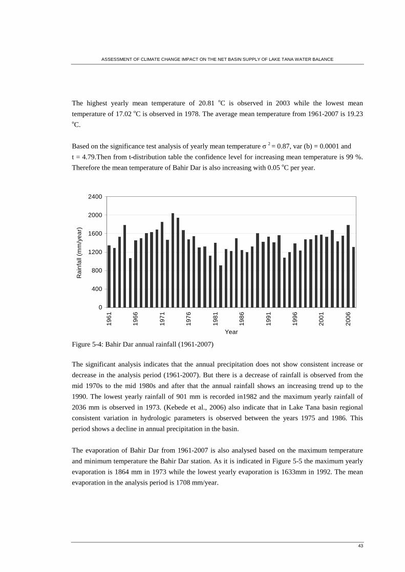
ASSESSMENT OF CLIMATE CHANGE IMPACT ON THE NET BASIN SUPPLY OF LAKE TANA WATER BALANCE
43
The highest yearly mean temperature of 20.81 oC is observed in 2003 while the lowest mean
temperature of 17.02 oC is observed in 1978. The average mean temperature from 1961-2007 is 19.23 oC.
Based on the significance test analysis of yearly mean temperature σ 2 = 0.87, var (b) = 0.0001 and
t = 4.79.Then from t-distribution table the confidence level for increasing mean temperature is 99 %.
Therefore the mean temperature of Bahir Dar is also increasing with 0.05 oC per year.
0
400
800
1200
1600
2000
2400
1961
1966
1971
1976
1981
1986
1991
1996
2001
2006
Year
Rai
nfa
ll (m
m/y
ear)
Figure 5-4: Bahir Dar annual rainfall (1961-2007)
The significant analysis indicates that the annual precipitation does not show consistent increase or
decrease in the analysis period (1961-2007). But there is a decrease of rainfall is observed from the
mid 1970s to the mid 1980s and after that the annual rainfall shows an increasing trend up to the
1990. The lowest yearly rainfall of 901 mm is recorded in1982 and the maximum yearly rainfall of
2036 mm is observed in 1973. (Kebede et al., 2006) also indicate that in Lake Tana basin regional
consistent variation in hydrologic parameters is observed between the years 1975 and 1986. This
period shows a decline in annual precipitation in the basin.
The evaporation of Bahir Dar from 1961-2007 is also analysed based on the maximum temperature
and minimum temperature the Bahir Dar station. As it is indicated in Figure 5-5 the maximum yearly
evaporation is 1864 mm in 1973 while the lowest yearly evaporation is 1633mm in 1992. The mean
evaporation in the analysis period is 1708 mm/year.

ASSESSMENT OF CLIMATE CHANGE IMPACT ON THE NET BASIN SUPPLY OF LAKE TANA WATER BALANCE
44
1500
1550
1600
1650
1700
1750
1800
1850
190019
61
1964
1967
1970
1973
1976
1979
1982
1985
1988
1991
1994
1997
2000
2003
2006
year
Eva
pora
tion
(mm
/yea
r)
Figure 5-5: Bahir Dar yearly evaporation
Table 5-1: Yearly increase of temperature using significance test from 1961-2007
Station name Maximum Temperature
( oC )
Minimum Temperature
(oC )
Mean Temperature
( oC )
Bahir Dar 0.07 0.026 0.05
Gonder 0.03 0.026 0.03
Debre Markos 0.05 0.016 0.04
The significance level of maximum, minimum and mean temperature for all the station is greater than
90 %. Therefore it is confident that the maximum and the minimum temperature of the present are
higher than the past periods.
5.2. Climate model output
5.2.1. Selected predictor variables
The selected predictor variables should be physically and conceptually sensible, strongly and
consistently correlated with the predictand and realistically modelled by GCMs. For precipitation
downscaling it is also recommended that the selected predictors contain variables describing
atmospheric circulation, thickness and stability and moisture content (Dawson and Wilbey, 2007).
Considering the above criteria daily data of surface divergent (ncepp_zhaf), 500hpa geo potential
height (ncepp500af) and mean temperature at 2 meter height (nceptemp) are selected for downscaling
of maximum and minimum temperature for all station used in the SDSM. For precipitation the
Surface divergent (ncepp_zhaf) and relative humidity at 500hpa (ncepr_500af) are selected.

ASSESSMENT OF CLIMATE CHANGE IMPACT ON THE NET BASIN SUPPLY OF LAKE TANA WATER BALANCE
45
Large scale convection over the warmer tropical ocean provides an important portion of the driving
energy for the general circulation of the atmosphere. The analysis of regional associations between
ocean temperature, surface wind divergence and convection produces two important phenomena. The
convergence zone is promoted by warm (> 28 oC) equatorial sea surface temperature (SST) while the
divergence zone is a result of subdued convection caused by colder SST (< 24 oC). The intertropical
convergent zone (ITCZ), which forms the zonal belt a few degrees to the north and south of the
equator, is best example of atmospheric convergences which drive the Hadley circulation. The
position of these zones (convergent and divergent) migrates seasonally and they exhibit inter annual
variation, which have a major effect on local precipitations (Luis and Pandey, 2005).
The predictor variables selected for each downscaling process conducted in this study are
summarized in Table 5-2, Table 5-3 and Table 5-4.
Table 5-2: List of predictor variables that give good correlation with Bahir Dar climate data Maximum temperature Minimum temperature Rainfall
predictors
Partial
r
P
value predictors
Partial
r
P
value predictors
Partial
r
P
value
ncepp_zhaf -0.367 0.00 ncepp_zhaf 0.542 0.00 ncepp_zhaf 0.251 0.00
ncepp500af 0.305 0.00 ncepp_500af 0.243 0.00 ncepr_500af 0.122 0.00
nceptemp 0.56 0.00 ncepp_temp 0.195 0.00
Table 5-3: List of predictor variables that give good correlation with Gonder climate data
Table 5-4: List of predictor variables that give good correlation with Debre Markos climate data
Where: The partial r is the correlation of the predicators with the predictand and P value is the
correlation of the predicators between each others.
Maximum temperature Minimum temperature Rainfall
predictors Partial r
P
value predictors Partial r
P
value predictors Partial r
P
value
ncepp_zhaf -0.566 0.00 ncepp_zhaf 0.249 0.00 ncepp_zhaf 0.278 0.00
ncepp500af -0.257 0.42 ncepp500af 0.131 0.00 ncepr_500af 0.101 0.00
nceptemp 0.545 0.00 ncepp_temp 0.381 0.00
Maximum temperature Minimum temperature Rainfall
predictors Partial r P value predictors Partial r
P value predictors Partial r
P value
ncepp_zhaf -0.548 0.00 ncepp_zhaf 0.334 0.00 ncepp_zhaf 0.261 0.00
ncepp500af -0.357 0.00 ncepp500af 0.204 0.00 ncepr_500af 0.157 0.00
nceptemp 0.576 0.00 ncepp_temp 0.322 0.00

ASSESSMENT OF CLIMATE CHANGE IMPACT ON THE NET BASIN SUPPLY OF LAKE TANA WATER BALANCE
46
5.2.2. Scenario developed for the baseline period
The IPCC recommends the 1961-1990 years as climatological baseline period in impact assessment.
Therefore the downscaling is done from 1961-1990 with A2 and B2 scenario outputs and the result is
compared to observed data of maximum temperature, minimum temperature and rainfall. The
monthly, the seasonal and the annual simulation for the baseline period is computed to compare the
result with the actual data. The wet season is from June to September and the dry season is from
October to February. The downscaling result for Gonder station is discussed below:
I. Maximum temperature
The actual and modelled result of maximum temperature indicates that the lowest monthly maximum
temperature is observed in July and August while the highest is observed in March and April. The wet
season has low maximum temperature than the dry season of the year because of rainfall and cloud
cover.
0
5
10
15
20
25
30
35
40
Janu
ary
Feb
ruar
y
Mar
ch
Apr
il
May
June
July
Aug
ust
Sep
tem
ber
Oct
ober
Nov
embe
r
Dec
embe
r
Wet
Sea
son
Dry
Sea
son
Ann
ual
Time
Tm
ax (
o C)
ActualHadCM3B2aHadCM3A2a
Figure 5-6: Observed and simulated maximum temperature for Gonder station (1961-1990).
As indicated in Figure 5-6 the downscaling result of maximum temperature with HadCM3A2a and
HadCM3B2a scenario output do not show much difference in the actual and modelled result. The
model error which is the difference of the observed and the simulated maximum temperature indicates
that the maximum absolute error is 0.24 oC in the month of September with HadCM3B2a scenario
output and the minimum is 0.03 oC in the month of April. Seasonally high model error is observed in
the wet season than dry seasons .The seasonal model error is general less than the monthly model
error. Generally no significant model error is observe in both scenario output for the whole months in
the analysis period then it is possible to conclude that the SDSM is able to simulate the maximum
temperature.

ASSESSMENT OF CLIMATE CHANGE IMPACT ON THE NET BASIN SUPPLY OF LAKE TANA WATER BALANCE
47
0.00
0.05
0.10
0.15
0.20
0.25
0.30
Janu
ary
Feb
ruar
y
Mar
ch
Apr
il
May
June
July
Aug
ust
Sep
tem
ber
Oct
ober
Nov
embe
r
Dec
embe
r
Wet
Sea
son
Dry
Sea
son
Ann
ual
Time
Mod
el e
rror
(o C)
HadCM3B2a
HadCM3A2a
Figure 5-7: Absolute model error of maximum temperature (1961-199)
0
1
2
3
4
5
Janu
ary
Feb
ruar
y
Mar
ch
Apr
il
May
June
July
Aug
ust
Sep
tem
ber
Oct
ober
Nov
embe
r
Dec
embe
r
Wet
Sea
son
Dry
Sea
son
Ann
ual
Time
Var
ianc
e (o C
) 2
actual
HadCM3A2a
HadCM3B2a
Figure 5-8: Variance of downscaled and actual maximum temperature (1961-1990)
Figure 5-8 also shows that the monthly and seasonal variability of maximum temperature for both
scenario output is almost similar to the observed variability of maximum temperature except a little

ASSESSMENT OF CLIMATE CHANGE IMPACT ON THE NET BASIN SUPPLY OF LAKE TANA WATER BALANCE
48
deviation from August to September and April. This indicates the model result follows the trend of the
actual maximum temperature.
II. Minimum temperature
Like maximum temperature the statistical downscaling model is able to reproduce the actual minimum
temperature except for a slight underestimation in the month of February and March. The model error
indicated in Figure 5-10 shows that the error in minimum temperature is less as compared to the
maximum temperature. Maximum error is observed in February, May and September while the error
in October is almost negligible for both scenario outputs.
0
3
6
9
12
15
18
21
Janu
ary
Feb
ruar
y
Mar
ch
Apr
il
May
June
July
Aug
ust
Sep
tem
ber
Oct
ober
Nov
embe
r
Dec
embe
r
Wet
Sea
son
Dry
Sea
son
Ann
ual
Time
Tm
in (
o C)
ActualHadCM3A2aHadCM3B2a
Figure 5-9: Observed and simulated minimum temperature for Gonder station (1961-1990).

ASSESSMENT OF CLIMATE CHANGE IMPACT ON THE NET BASIN SUPPLY OF LAKE TANA WATER BALANCE
49
0.00
0.04
0.08
0.12
0.16
0.20
Janu
ary
Feb
ruar
y
Mar
ch
Apr
il
May
June
July
Aug
ust
Sep
tem
ber
Oct
ober
Nov
embe
r
Dec
embe
r
Wet
Sea
son
Dry
sea
son
Ann
ual
Time
Mod
el e
rror
(o C
)
HadCM3A2a
HadCM3B2a
Figure 5-10: Absolute model error of minimum temperature
0
1
2
3
4
5
Janu
ary
Feb
ruar
y
Mar
ch
Apr
il
May
June
July
Aug
ust
Sep
tem
ber
Oct
ober
Nov
embe
r
Dec
embe
r
Wet
Sea
son
Dry
Sea
son
Ann
ual
Time
Var
ianc
e (
o C)
2
actual
HadCM3A2aHadCM3B2a
Figure 5-11: Variance of downscaled and actual minimum temperature
Like the maximum temperature the monthly and seasonal variably of the actual and modelled
minimum temperature is similar. High variance in minimum temperature exists in February and
March while in July and August the variance has the lowest value.
III. Precipitation
As it is shown in Figure 5-12 the statistical downscaling model is able to simulate the actual
precipitation except for a slight over estimation in September, October and May and a slight under

ASSESSMENT OF CLIMATE CHANGE IMPACT ON THE NET BASIN SUPPLY OF LAKE TANA WATER BALANCE
50
estimation on the month of July and June. But the simulation result of precipitation with the statistical
downscaling model is less accurate as compared to the maximum and minimum temperature. The
average monthly model error is 8.47 and 9.01 mm and the annual model error is 46 mm and 50 mm
for HadCM3A2a and HadCM3B2a scenario output respectively. High model error occurred in wet
season than the dry season of the year. Even though some difference between the observed and the
simulated precipitation, the monthly and seasonal variability is in good agreement and SDSM able to
replicate the precipitation in acceptable limit.
0
50
100
150
200
250
300
350
Janu
ary
Feb
ruar
y
Mar
ch
Apr
il
May
June
July
Aug
ust
Sep
tem
ber
Oct
ober
Nov
embe
r
Dec
embe
r
Month
Pre
cipi
tatio
n (m
m/m
onth
) ActualHadCM3A2aHadCM3B2a
Figure 5-12: Observed and simulated precipitation for Gonder station (1961-1990)
Seasonally as shown in the Figure 5-13 the precipitation amount in wet and dry seasons are slightly
over estimated compared to the actual. Therefore the annual precipitation with both HadCM3A2a and
HadCM3B2a scenario output is higher than the actual precipitation.
0
200
400
600
800
1000
1200
1400
1600
Wet Season Dry Season Annual
Season
Tot
al a
vera
ge p
reci
ptat
ion
(mm
)
Actual HadCM3A2a HadCM3B2a
Figure 5-13: Average seasonal precipitation of Gonder station (1961-1990)

ASSESSMENT OF CLIMATE CHANGE IMPACT ON THE NET BASIN SUPPLY OF LAKE TANA WATER BALANCE
51
0
10
20
30
40
50
60
Janu
ary
Feb
ruar
y
Mar
ch
Apr
il
May
June
July
Aug
ust
Sep
tem
ber
Oct
ober
Nov
embe
r
Dec
embe
r
Wet
Sea
son
Dry
Sea
son
Ann
ual
Time
Mod
el e
rror
(m
m)
HadCM3A2aHadCM3B2a
Figure 5-14: Absolute model error of precipitation (1961-1990)
0
20
40
60
80
100
120
140
160
180
200
Janu
ary
Feb
ruar
y
Mar
ch
Apr
il
May
June
July
Aug
ust
Sep
tem
ber
Oct
ober
Nov
embe
r
Dec
embe
r
Wet
Sea
son
Dry
Sea
son
Ann
ual
Time
Var
ianc
e (m
m)
2
actual
HadCM3A2a
HadCM3B2a
Figure 5-15: Variance of downscaled and actual precipitation (1961-1990)
The simulation result of the maximum temperature, minimum temperature and precipitation of Bahir
Dar and Debre Markos stations for the baseline period with HadCM3A2a and HadCM3B2a scenario
output is also well. Like the result obtained for Gonder station the SDSM well simulate the maximum
temperature and minimum temperature than precipitation for the other stations.
Generally maximum temperature and the minimum temperature have better agreement with the
observed result than the precipitation. The simulation of precipitation though showed a relatively
lesser agreement as compared to the maximum and minimum temperature, but the result is acceptable

ASSESSMENT OF CLIMATE CHANGE IMPACT ON THE NET BASIN SUPPLY OF LAKE TANA WATER BALANCE
52
due to the fact that precipitation is the conditional process. As discussed before, conditional process
like precipitation are dependant on other intermediate processes like on the occurrence of humidity,
cloud cover, and wet day occurrence. Unconditional process like temperature; however, are not
regulated by other intermediate process. In addition, as indicated in the SDSM manual (Wilby &
Dawson 2007), local temperature are largely determined by regional forcing whereas precipitation
series display more “noise” arising from local factor. Hence larger differences can be observed in
precipitation ensemble members than that of temperature.
5.2.3. Downscaling of GCM for future period
Once the downscaling model has been setup the next step is to use the SDSM to downscale for the
future period based on the HadCM3A2a and HadCM3B2a scenario outputs. The Precipitation and
temperature downscaling is done for each of the three periods 2020s (2010-2039), 2040s (2040-2069)
and 2070s (2070-2099). The respective average monthly, seasonal and annual change from the
baseline period for both A2 and B2 scenarios were calculated for maximum and minimum
temperature. For precipitation the monthly, seasonal and annual precipitation amount for the baseline
and future scenario period is calculated. The change in temperature and the precipitation amount for
Gonder station is discussed below. The result obtained for Bahir Dar and Debre Markos station are
presented in the Appendix F.
I. Maximum temperature
The downscaling of maximum temperature in the future period as it is indicated in Figure 5-17 and
Figure 5-17 shows that the average increase of temperature in 2020s is 0.4 oC and in 2040s it is further
increases to 0.7 oC and 0.8 oC for A2 and B2 scenario respectively. In 2070s the increase is 1.15 oC
and 1.47 oC for A2 and B2 scenario. The 2070s increase is higher than for both 2020s and 2040s
increase. This shows the maximum temperature has an increase trend in the future period. The change
in maximum temperature from the baseline period is high in wet season for both scenarios. Seasonally
high maximum temperature change occurred in the wet season while the maximum temperature
change in dry season shows minor increment.

ASSESSMENT OF CLIMATE CHANGE IMPACT ON THE NET BASIN SUPPLY OF LAKE TANA WATER BALANCE
53
0
0.5
1
1.5
2
2.5
3
3.5
Janu
ary
Feb
ruar
y
Mar
ch
Apr
il
May
June
July
Aug
ust
Sep
tem
ber
Oct
ober
Nov
embe
r
Dec
embe
r
Wet
Sea
son
Dry
Sea
son
Ann
ual
Time
Tem
pera
ture
cha
nge(
o C)
2010-20392040-20692070-2099
Figure 5-16: Average monthly Maximum temperature change from the baseline period with
HadCM3B2a scenario output (Gonder station)
0
0.5
1
1.5
2
2.5
3
3.5
4
Janu
ary
Feb
ruar
y
Mar
ch
Apr
il
May
June
July
Aug
ust
Sep
tem
ber
Oct
ober
Nov
embe
r
Dec
embe
r
Wet
Sea
son
Dry
Sea
son
Ann
ual
Time
Tem
pera
ture
cha
nge
( o C) 2010-2039
2040-20692070-2099
Figure 5-17: Average monthly maximum temperature change from the baseline period for HadCM3A2a scenario outputs (Gonder station)

ASSESSMENT OF CLIMATE CHANGE IMPACT ON THE NET BASIN SUPPLY OF LAKE TANA WATER BALANCE
54
y = 0.019x - 37.734
R2 = 0.92
y = 0.0109x - 21.513
R2 = 0.98
0
0.5
1
1.5
2
2.5
3
1990 2000 2010 2020 2030 2040 2050 2060 2070 2080 2090
Scenario year
Tm
ax c
hang
e ( o C
)
Wet Season(JJAS)Dry Season (ONDJF)Linear (Wet Season(JJAS))Linear (Dry Season (ONDJF))
Figure 5-18: Seasonal maximum temperature change in the current and future time for Gonder station (HadCM3A2a)
y = 0.0128x - 25.246
R2 = 0.92
y = 0.0065x - 12.801
R2 = 0.96
0.0
0.5
1.0
1.5
2.0
2.5
1990 2000 2010 2020 2030 2040 2050 2060 2070 2080 2090
Scenario year
Tm
ax c
hang
e( o C
)
Wet season (JJAS) Dry Season (ONDJF)Linear (Wet season (JJAS) )Linear (Dry Season (ONDJF))
Figure 5-19: Seasonal maximum temperature change in the current and future time for Gonder station
(HadCM3B2a)
In Figure 5-19 and Figure 5-19 the scenario year 2000, 2020, 2050 and 2080 indicates 1991-2007,
2010-2039, 2040-2069 and 2070-2099 year respectively. The 2000 (1991-2007) seasonally changes
for minimum temperature, maximum temperature and rainfall is calculated with the observed data.
Based on monthly average maximum temperature of the above scenario years the seasonal changes
with respect to the baseline period is computed. The result indicates that both scenario outputs have a
high maximum temperature changes in the wet season than in the dry season. But the overall increase

ASSESSMENT OF CLIMATE CHANGE IMPACT ON THE NET BASIN SUPPLY OF LAKE TANA WATER BALANCE
55
in maximum temperature is higher with HadCM3A2a scenario output than the output from
HadCM3B2a scenario.
II. Minimum temperature
Like the average monthly maximum temperature the average monthly minimum temperature also
shows an increment in all months of the year. Figure 5-21 and Figure 5-21 indicates that the increase
in minimum temperature in 2020s is 0.20 oC and 0.24 oC for B2 and A2 scenario respectively. This
change increases to 0.41oC and 0.50 oC in 2040s and it is further increases to 0.61oC and 0.84 oC in
2070s for B2 and A2 scenario respectively .High minimum temperature change is observed in month
of February, March and December. Seasonally contrary to the average maximum temperature change
high minimum temperature change occurred in dry season of the year while the minimum temperature
change in the wet season shows small increment.
0
0.5
1
1.5
2
2.5
3
Janu
ary
Feb
ruar
y
Mar
ch
Apr
il
May
June
July
Aug
ust
Sep
tem
ber
Oct
ober
Nov
embe
r
Dec
embe
r
Wet
Sea
son
Dry
Sea
son
Ann
ual
Time
Tem
pera
ture
cha
nge
( o C)
2010-20392040-20692070-2099
Figure 5-20: Average minimum temperature change from the baseline period for HadCM3A2a
scenario output (Gonder station)

ASSESSMENT OF CLIMATE CHANGE IMPACT ON THE NET BASIN SUPPLY OF LAKE TANA WATER BALANCE
56
0
0.5
1
1.5
2Ja
nuar
y
Feb
ruar
y
Mar
ch
Apr
il
May
June
July
Aug
ust
Sep
tem
ber
Oct
ober
Nov
embe
r
Dec
embe
r
Wet
Sea
son
Dry
Sea
son
Ann
ual
Time
Tem
pera
ture
cha
nge(
o C)
2010-20392040-20692070-2099
Figure 5-21: Average minimum temperature change from the baseline period for HadCM3B2a
scenario output (Gonder station).
y = 0.006x - 12.2
R2 = 0.95
y = 0.003x - 5.6
R2 = 0.93
0
0.2
0.4
0.6
0.8
1
1.2
1990 2000 2010 2020 2030 2040 2050 2060 2070 2080 2090
Scenario year
Tm
in c
hang
e ( o C
)
Wet Season (JJAS) Dry Season (ONDJF)
Linear (Dry Season (ONDJF)) Linear (Wet Season (JJAS))
Figure 5-22: Seasonal minimum temperature change in the current and future time for Gonder station
(HadCM3B2a)

ASSESSMENT OF CLIMATE CHANGE IMPACT ON THE NET BASIN SUPPLY OF LAKE TANA WATER BALANCE
57
y = 0.009x - 17.03
R2 = 0.93
y = 0.0034x - 6.5
R2 = 0.87
0
0.2
0.4
0.6
0.8
1
1.2
1.4
1.6
1990 2000 2010 2020 2030 2040 2050 2060 2070 2080 2090
Scenario year
Tm
in c
hang
e ( o C
)
Wet Season (JJAS) Dry Season (ONDJF)Linear (Dry Season (ONDJF)) Linear (Wet Season (JJAS))
Figure 5-23: Seasonal minimum temperature change in the current and future time for Gonder station
(HadCM3A2a)
As it is observed in Figure 5-23 and Figure 5-3 the minimum temperature change in dry season is
higher than the wet season for all scenario years. The increase of minimum temperature with both
scenario output shows an increasing trend as compared to the baseline period for both dry season and
wet season.
III. Evaporation
The evaporation of Gonder is computed with the maximum and minimum temperature for the analysis
period. Hargreaves method is applicable for the evaporation estimation since no sufficient climate
data are available for the other methods. The increase in maximum and minimum temperature with
both scenario output results in an increase in evaporation of the catchment. As it is observed in Figure
5-24 the evaporation shows an increasing trend as compared to the baseline period. But the
evaporation with HadCM3A2a scenario output is higher than HadCM3B2a scenario output. The
annual mean evaporation is 1660 mm, 1681mm and 1711mm for the period of 2010-2039, 2040-2069
and 2070-2099 respectively with HadCM3B2a scenario output. The mean annual evaporation with
HadCM3A2a scenario output is 1658 mm, 1691 mm and 1739 mm for the period of 2010-2039, 2040-
2069 and 2070-2099 respectively. The baseline period and the 1991-2007 annual mean evaporation
are calculated by the observed data with Hargreaves method and it is estimated to be 1636mm and
1648mm respectively.

ASSESSMENT OF CLIMATE CHANGE IMPACT ON THE NET BASIN SUPPLY OF LAKE TANA WATER BALANCE
58
y = 1.0906x - 532.59
R2 = 0.90
y = 0.8004x + 47.552
R2 = 0.96
1620
1640
1660
1680
1700
1720
1740
1760
1970 1980 1990 2000 2010 2020 2030 2040 2050 2060 2070 2080
Scenario year
Eva
pora
tion
(mm
/yea
r)
HadCM3A2a HadCM3B2a Linear (HadCM3A2a) Linear (HadCM3B2a)
Figure 5-24: Annual average evaporation for Gonder station
IV. Precipitation
The monthly average precipitation is increasing by 4.8 % and 7.4% in 2020s for A2 and B2 scenarios
with reference to the baseline period precipitation. The average increase of monthly precipitation is
7.2 % and 7.8 % in 2040s and 9.4 % and 8.9 % in 2070s for A2 and B2 scenario respectively.
0
50
100
150
200
250
300
350
Janu
ary
Feb
ruar
y
Mar
ch
Apr
il
May
June
July
Aug
ust
Sep
tem
ber
Oct
ober
Nov
embe
r
Dec
embe
r
Month
Pre
cipt
atio
n (m
m/m
onth
)
Actual2010-2039
2040-20692070-2099
Figure 5-25: Monthly average precipitation downscaled from HadCM3B2a scenario output (Gonder
station)
A higher increase in precipitation is occurred on the month of August and September which are the
part of the wet season. As it is observed in Figure 5-29 and Figure 5-28 for both HadCM3A2a and

ASSESSMENT OF CLIMATE CHANGE IMPACT ON THE NET BASIN SUPPLY OF LAKE TANA WATER BALANCE
59
HadCM3B2a scenario outputs the wet season shows an increasing trend for all future periods. The
wet season has 75% contribution for the annual rainfall in the Lake Tana basin therefore the annual
rainfall also shows an increasing trend in the future period. But the increase in precipitation for
HadCM3A2a scenario output is slightly higher than the precipitation obtained from HadCM3B2a
scenario.
0
50
100
150
200
250
300
350
Janu
ary
Feb
ruar
y
Mar
ch
Apr
il
May
June
July
Aug
ust
Sep
tem
ber
Oct
ober
Nov
embe
r
Dec
embe
r
Month
Pre
cipt
atio
n (m
m/m
onth
)
Actual2010-20392040-20692070-2099
Figure 5-26: Monthly average precipitation downscaled from HadCM3A2a scenario output
(Gonder station)
Figure 5-27: Mean daily precipitation in Ethiopian Highland under the present and future period
(deBoer, 2007)
The climate change and impact study in the Blue Nile region by deBoer (2007) indicates that there is a
shift of the rainy season towards the end of the year and there is an increase of total precipitation in
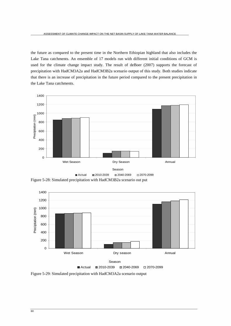
ASSESSMENT OF CLIMATE CHANGE IMPACT ON THE NET BASIN SUPPLY OF LAKE TANA WATER BALANCE
60
the future as compared to the present time in the Northern Ethiopian highland that also includes the
Lake Tana catchments. An ensemble of 17 models run with different initial conditions of GCM is
used for the climate change impact study. The result of deBoer (2007) supports the forecast of
precipitation with HadCM3A2a and HadCM3B2a scenario output of this study. Both studies indicate
that there is an increase of precipitation in the future period compared to the present precipitation in
the Lake Tana catchments.
0
200
400
600
800
1000
1200
1400
Wet Season Dry Season Annual
Season
Pre
cipt
atio
n (m
m)
Actual 2010-2039 2040-2069 2070-2099
Figure 5-28: Simulated precipitation with HadCM3B2a scenario out put
0
200
400
600
800
1000
1200
1400
Wet Season Dry season Annual
Season
Pre
cipt
atio
n (m
m)
Actual 2010-2039 2040-2069 2070-2099
Figure 5-29: Simulated precipitation with HadCM3A2a scenario output

ASSESSMENT OF CLIMATE CHANGE IMPACT ON THE NET BASIN SUPPLY OF LAKE TANA WATER BALANCE
61
y = 0.9845x - 840.61
R2 = 0.78
y = 1.1753x - 1225.6
R2 = 0.92
1080
1100
1120
1140
1160
1180
1200
1220
1240
1260
1280
1970 1980 1990 2000 2010 2020 2030 2040 2050 2060 2070 2080 2090
Scenario year
Pre
cipt
atio
n (m
m)
HadCM3A2aHadCM3B2aLinear (HadCM3B2a)Linear (HadCM3A2a)
Figure 5-30: Annual average precipitation for Gonder station
The annual mean precipitation for both scenarios indicates that there is an increase in precipitation in
future scenario period mainly due to an increasing of precipitation in the wet season. As it is observed
in Figure 5-30 the annual average precipitation in 2050 (2040-2069) and 2080 (2070-2099) for
HadCM3A2a scenario output is higher than the HadCM3B2a scenario output while in 2020 (2010-
2039) the precipitation of HadCMEB2a scenario is higher than the HadCM3A2a scenario. As it is
observed in Figure 5-31 the observed annual and seasonal mean of precipitation in 2000 (1991-2007)
is less compared to mean of the baseline and future scenario year precipitation. But the forecasted
precipitation in the future scenario period is higher than the observed precipitation.
y = 0.3059x + 253.16
R2 = 0.72
y = 0.4689x - 69.869
R2 = 0.79
840
850
860
870
880
890
900
910
920
930
1970 1980 1990 2000 2010 2020 2030 2040 2050 2060 2070 2080 2090
Scenario year
Pre
cipt
atio
n (m
m)
HadCM3A2aHadCM3B2aLinear (HadCM3A2a)Linear (HadCM3B2a)
Figure 5-31: Wet Season precipitation for Gonder station
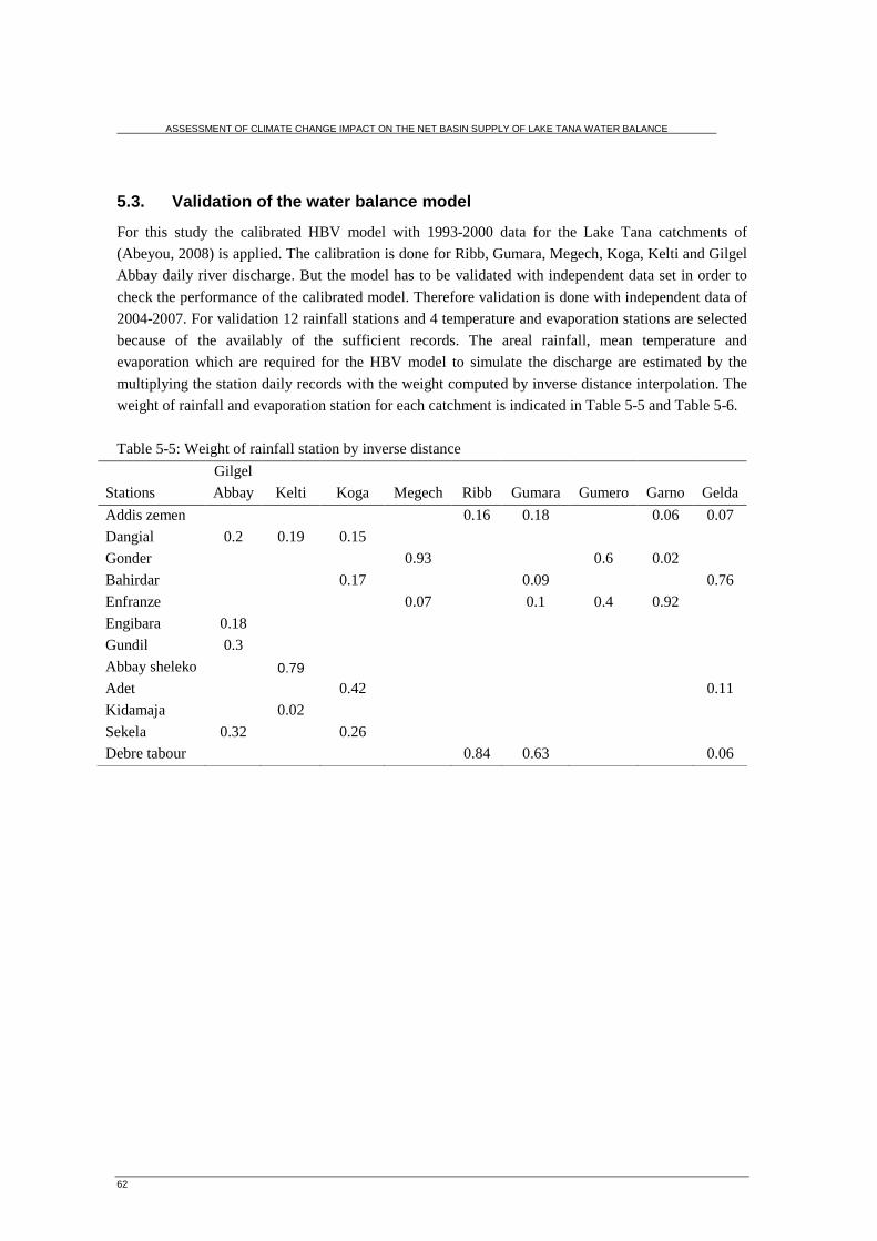
ASSESSMENT OF CLIMATE CHANGE IMPACT ON THE NET BASIN SUPPLY OF LAKE TANA WATER BALANCE
62
5.3. Validation of the water balance model
For this study the calibrated HBV model with 1993-2000 data for the Lake Tana catchments of
(Abeyou, 2008) is applied. The calibration is done for Ribb, Gumara, Megech, Koga, Kelti and Gilgel
Abbay daily river discharge. But the model has to be validated with independent data set in order to
check the performance of the calibrated model. Therefore validation is done with independent data of
2004-2007. For validation 12 rainfall stations and 4 temperature and evaporation stations are selected
because of the availably of the sufficient records. The areal rainfall, mean temperature and
evaporation which are required for the HBV model to simulate the discharge are estimated by the
multiplying the station daily records with the weight computed by inverse distance interpolation. The
weight of rainfall and evaporation station for each catchment is indicated in Table 5-5 and Table 5-6.
Table 5-5: Weight of rainfall station by inverse distance
Stations
Gilgel
Abbay Kelti Koga Megech Ribb Gumara Gumero Garno Gelda
Addis zemen 0.16 0.18 0.06 0.07
Dangial 0.2 0.19 0.15
Gonder 0.93 0.6 0.02
Bahirdar 0.17 0.09 0.76
Enfranze 0.07 0.1 0.4 0.92
Engibara 0.18
Gundil 0.3
Abbay sheleko 0.79
Adet 0.42 0.11
Kidamaja 0.02
Sekela 0.32 0.26
Debre tabour 0.84 0.63 0.06
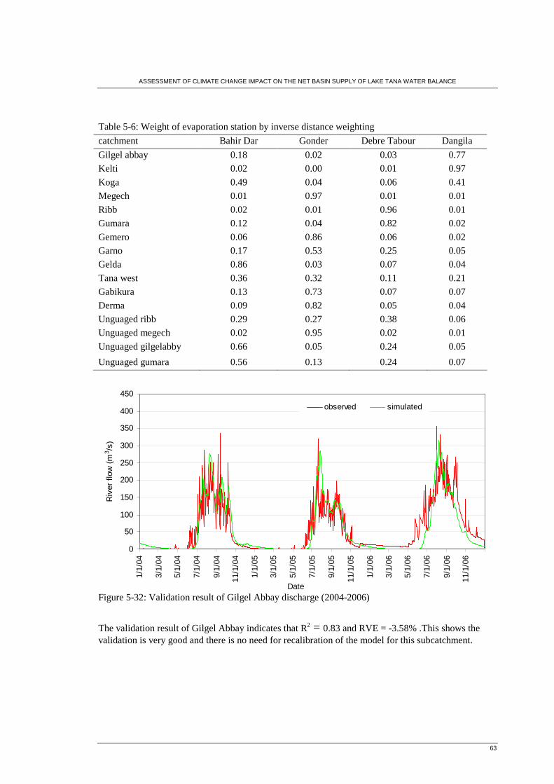
ASSESSMENT OF CLIMATE CHANGE IMPACT ON THE NET BASIN SUPPLY OF LAKE TANA WATER BALANCE
63
Table 5-6: Weight of evaporation station by inverse distance weighting
catchment Bahir Dar Gonder Debre Tabour Dangila
Gilgel abbay 0.18 0.02 0.03 0.77
Kelti 0.02 0.00 0.01 0.97
Koga 0.49 0.04 0.06 0.41
Megech 0.01 0.97 0.01 0.01
Ribb 0.02 0.01 0.96 0.01
Gumara 0.12 0.04 0.82 0.02
Gemero 0.06 0.86 0.06 0.02
Garno 0.17 0.53 0.25 0.05
Gelda 0.86 0.03 0.07 0.04
Tana west 0.36 0.32 0.11 0.21
Gabikura 0.13 0.73 0.07 0.07
Derma 0.09 0.82 0.05 0.04
Unguaged ribb 0.29 0.27 0.38 0.06
Unguaged megech 0.02 0.95 0.02 0.01
Unguaged gilgelabby 0.66 0.05 0.24 0.05
Unguaged gumara 0.56 0.13 0.24 0.07
0
50
100
150
200
250
300
350
400
450
1/1/
04
3/1/
04
5/1/
04
7/1/
04
9/1/
04
11/1
/04
1/1/
05
3/1/
05
5/1/
05
7/1/
05
9/1/
05
11/1
/05
1/1/
06
3/1/
06
5/1/
06
7/1/
06
9/1/
06
11/1
/06
Date
Riv
er f
low
(m
3 /s)
observed simulated
Figure 5-32: Validation result of Gilgel Abbay discharge (2004-2006)
The validation result of Gilgel Abbay indicates that R2 = 0.83 and RVE = -3.58% .This shows the validation is very good and there is no need for recalibration of the model for this subcatchment.
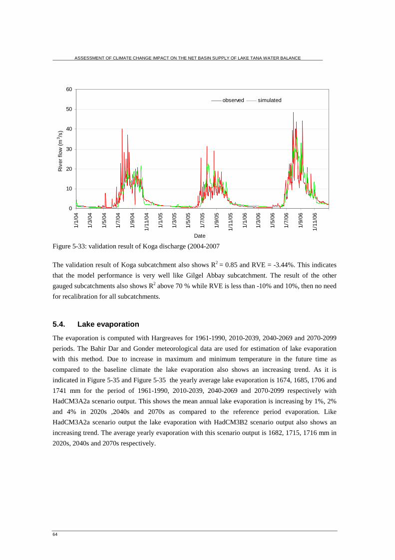
ASSESSMENT OF CLIMATE CHANGE IMPACT ON THE NET BASIN SUPPLY OF LAKE TANA WATER BALANCE
64
0
10
20
30
40
50
60
1/1/
04
1/3/
04
1/5/
04
1/7/
04
1/9/
04
1/11
/04
1/1/
05
1/3/
05
1/5/
05
1/7/
05
1/9/
05
1/11
/05
1/1/
06
1/3/
06
1/5/
06
1/7/
06
1/9/
06
1/11
/06
Date
Riv
er f
low
(m
3 /s)
observed simulated
Figure 5-33: validation result of Koga discharge (2004-2007
The validation result of Koga subcatchment also shows R2 = 0.85 and RVE = -3.44%. This indicates
that the model performance is very well like Gilgel Abbay subcatchment. The result of the other
gauged subcatchments also shows R2 above 70 % while RVE is less than -10% and 10%, then no need
for recalibration for all subcatchments.
5.4. Lake evaporation
The evaporation is computed with Hargreaves for 1961-1990, 2010-2039, 2040-2069 and 2070-2099
periods. The Bahir Dar and Gonder meteorological data are used for estimation of lake evaporation
with this method. Due to increase in maximum and minimum temperature in the future time as
compared to the baseline climate the lake evaporation also shows an increasing trend. As it is
indicated in Figure 5-35 and Figure 5-35 the yearly average lake evaporation is 1674, 1685, 1706 and
1741 mm for the period of 1961-1990, 2010-2039, 2040-2069 and 2070-2099 respectively with
HadCM3A2a scenario output. This shows the mean annual lake evaporation is increasing by 1%, 2%
and 4% in 2020s ,2040s and 2070s as compared to the reference period evaporation. Like
HadCM3A2a scenario output the lake evaporation with HadCM3B2 scenario output also shows an
increasing trend. The average yearly evaporation with this scenario output is 1682, 1715, 1716 mm in
2020s, 2040s and 2070s respectively.

ASSESSMENT OF CLIMATE CHANGE IMPACT ON THE NET BASIN SUPPLY OF LAKE TANA WATER BALANCE
65
1500
1550
1600
1650
1700
1750
1800
1850
1 3 5 7 9 11 13 15 17 19 21 23 25 27 29
Scenario year
Eva
pora
tion
(mm
/yea
r)
1961-19902010-20392040-20692070-2099
Figure 5-34: Lake Tana yearly evaporation with HadCM3B2a scenario output
1500
1550
1600
1650
1700
1750
1800
1850
1900
1 3 5 7 9 11 13 15 17 19 21 23 25 27 29
Scenario year
Eva
pora
tion
(mm
/yea
r)
1961-19902010-20392040-20692070-2099
Figure 5-35: Lake Tana yearly evaporation with HadCM3A2a scenario output
5.5. Lake precipitation
Lake Tana precipitation is one of the major components of the net basin supply and it is calculated
based on the Bahir Dar and Gonder stations. Both stations are relatively near to the lake and they have
sufficient data for downscaling of precipitation in the future scenario period then they are selected for
estimation of the lake precipitation for the current and future time period.

ASSESSMENT OF CLIMATE CHANGE IMPACT ON THE NET BASIN SUPPLY OF LAKE TANA WATER BALANCE
66
0
500
1000
1500
2000
2500
1 3 5 7 9 11 13 15 17 19 21 23 25 27 29
Scenario year
Pre
cipt
atio
n (m
m/y
ear)
1961-19902010-20392040-20692070-2099
Figure 5-36: Annual Precipitation of Lake Tana with HadCM3A2a scenario output
The annual lake precipitation is computed for HadCM3A2a and HadCM3B2a scenario outputs for the
three future time horizons and the result is compared to the baseline period in order to determine the
change. The result indicates that the mean annual lake precipitation is increasing by 8.54 %, 10.02 %
and 17.27 % for the 2020s, 2040s and 2070s as compared to the baseline period with HadCM3A2a
scenario output. The mean annual lake precipitation for the baseline period is 1312 mm/year.
600
900
1200
1500
1800
2100
1 3 5 7 9 11 13 15 17 19 21 23 25 27 29
Scnario year
Pre
cipt
atio
n (m
m/y
ear)
1961-19902010-20392040-20692070-2099
Figure 5-37: Annual lake precipitation with HadCM3B2a scenario output
The lake precipitation also computed with HadCM3B2a scenario output and the result indicates that
the mean annual precipitation increases by 3.68, 3.65 and 3.2 % respectively for 202s, 2040s and

ASSESSMENT OF CLIMATE CHANGE IMPACT ON THE NET BASIN SUPPLY OF LAKE TANA WATER BALANCE
67
2070s periods as compared to the 1961-1990 periods. The increase in precipitation with HadCM3B2a
scenario output is less as compared to the HadCM3A2a scenario output. This is because the Bahir Dar
and Gonder precipitation in the future period with HadCM3A2a scenario output is higher than that of
HadCM3B2a scenario output.
An increase in surface temperature in the future period leads to higher evaporation rates and enable
the atmosphere to transport higher amount of water vapour. Therefore the global hydrological cycle
will be accelerated (Menzel and Bürger, 2002). According to the Intergovrernmental Panel on Climate
Change (IPCC, 2001) an increasing in preciptation is likely to happen large contenintal area in the
tropics and at higher latitudes.
5.6. Net basin supply of Lake Tana water balance
After validation of the HBV model the next step is forecasting of the inflow to the Lake Tana based
on the observed and downscaled precipitation, temperature and evaporation of the three stations. The
net basin supply is then calculated based on the lake precipitation , lake evaporation and inflow to the
lake for baseline period and the other three future time periods 2020s (2101-2039), 2040s (2040-
2069) and 2070s (2070-2099).
0
500
1000
1500
2000
2500
3000
3500
4000
1 3 5 7 9 11 13 15 17 19 21 23 25 27 29
Scenario year
Inf
low
(m
m/y
ear)
1961-19902010-20392040-20692070-2099
Figure 5-38: Annual Lake Tana inflow with HadCM3A2a scenario output
The increase of inflow to the lake is due to increase in precipitation. As it is indicated in Figure 5-38
the minimum annual inflows are observed between 1979-1988 while the maximum inflows are
observed between 1973-1976 and 1963-1965 with HadCM3A2a scenario output.

ASSESSMENT OF CLIMATE CHANGE IMPACT ON THE NET BASIN SUPPLY OF LAKE TANA WATER BALANCE
68
0
500
1000
1500
2000
2500
3000
3500
1 3 5 7 9 11 13 15 17 19 21 23 25 27 29
Senario year
Inflo
w (
mm
/yea
r)
1961-19902010-20392040-20692070-2099
Figure 5-39: Annual lake inflow with HadCM3B2a scenario output
The annual inflow to the lake with HadCM3B2a scenario output also shows an increasing trend but as
compared to the HadCM3A2a scenario output the increase is less. This less inflow is due to the
decrease of downscaled precipitation of Bahir Dar, Gonder and Debre Markos with HadCM3B2a
scenario output than HadCM3A2a. The average annual inflows are increasing by 3.1, 1.1 and 2.5%
for 2020s, 2040s and 2070s periods respectively as compared to the baseline period.
0
500
1000
1500
2000
2500
3000
3500
4000
1 3 5 7 9 11 13 15 17 19 21 23 25 27 29
Scenario year
Net
bas
in s
upp
ly (
mm
/ye
ar)
1961-19902010-20392040-20692070-2099
Figure 5-40: Net basin supply of Lake Tana water balance with HadCM3A2a scenario output
The net basin supply of Lake Tana shows an increasing trend from the baseline period of 1961-1990.
The average annual net basin supply is 1801, 1783 and 1991mm/year for the period of 2010-2039,

ASSESSMENT OF CLIMATE CHANGE IMPACT ON THE NET BASIN SUPPLY OF LAKE TANA WATER BALANCE
69
2040-2069 and 2070-2099 respectively with HadCM3A2a scenario output and the baseline period net
basin supply is 1459 mm/year. The analysis of hydrology and water resources in on the Upper Blue
Nile river basin under climate change by Kim and Kaluaranchchi (2008) also indicates that there is
increasing of precipitation and runoff in Northern Amhara (North Ethiopia) which covers the Lake
Tana catchment, in the future scenario periods as compared to the base line period. Therefore both
result shows increase of precipitation and inflow in the Lake Tana basin for the future scenario
periods.
-0.2
0.3
0.8
1.3
1.8
Jan-
61
Jan-
63
Jan-
65
Jan-
67
Jan-
69
Jan-
71
Jan-
73
Jan-
75
Jan-
77
Jan-
79
Jan-
81
Jan-
83
Jan-
85
Jan-
87
Jan-
89
Month
Mon
thly
net
bas
in s
uppl
y (m
/mon
th)
Figure 5-41: Monthly Net basin supply with HadCM3A2a scenario output
The monthly net basin supply with HadCM3A2a scenario output indicates that the net basin supply is
high in the wet season from July to October while in the dry seasons from January to May it shows the
lowest value. During dry months the net basin supply becomes negative since lake evaporation is
higher than the sum of inflow to the lake and lake precipitation.
As it is shown in Figure 5-42 the net basin supply with HadCM3B2a scenario also indicates an
increasing trend like the HadCM3A2a scenario output compared to the baseline period. The mean
annual net basin supply is 1554, 1481, and 1530 mm/year for the period of 2010-2039, 2040-2069 and
2070-2099 respectively. But the increase in mean annual net basin supply is generally less as
compared to HadCM3A2a model because of decrease of the annual lake precipitation and lake inflow.
In A2 scenario the future world becomes warmer than the B2 scenario because of increasing CO2
concentration and hydrological cycle is likely to become more affected. Therefore the precipitation in
A2 scenario is higher than B2 scenario. This increase in precipitation causes an increase in stream
flow in future time periods and consequently the net basin supply become increase with A2 scenario
than B2 scenario.

ASSESSMENT OF CLIMATE CHANGE IMPACT ON THE NET BASIN SUPPLY OF LAKE TANA WATER BALANCE
70
0
500
1000
1500
2000
2500
3000
3500
1 3 5 7 9 11 13 15 17 19 21 23 25 27 29
Scenario year
Net
bas
in s
uppl
y (m
m/y
ear)
1961-19902010-20392040-20692070-2099
Figure 5-42: Annual net basin supply with HadCM3B2a scenario output
To analyse the effect of climate change on the net basin supply the mean monthly net basin supply for
both scenario out put is made beside the annual net basin supply. As it is indicated in Figure 5-43 and
Figure 5-44 the mean monthly net basin supply is 121.6, 129.5, 123.5 and 127.6 mm/ month for 1961-
190, 2010-2039, 2040-2069 and 2070-2099 with HadCM3B2a scenario output. Like the mean annual
net basin supply with this scenario the highest mean monthly net basin supply is observed in 2020s.
The mean monthly net basin supply with HadCMEA2a scenario output is 121.6, 150.1, 148.6 and 166
mm for the period of 1961-1990, 2010-2039, 2040-2069 and 2070-2099 respectively. For both
scenario output the mean monthly net basin supply shows an increasing trend as compared to the
baseline period.

ASSESSMENT OF CLIMATE CHANGE IMPACT ON THE NET BASIN SUPPLY OF LAKE TANA WATER BALANCE
71
-200
0
200
400
600
800
1000
Janu
ary
Feb
ruar
y
Mar
ch
Apr
il
May
June
July
Aug
est
Sep
tem
ber
Oct
obe
r
No
vem
ber
De
cem
ber
Month
Net
bas
in s
uppl
y (m
m/m
onth
) 1961-19902010-20392040-20692070-2099
Figure 5-43: Mean monthly net basin supply with HadCM3B2a scenario output
-200
0
200
400
600
800
1000
Janu
ary
Feb
ruar
y
Mar
ch
Apr
il
May
June
July
Aug
est
Sep
tem
ber
Oct
ober
Nov
embe
r
Dec
embe
r
Month
Net
bas
in s
uppl
y (m
m/m
onth
)
1961-19902010-20392040-20692070-2099
Figure 5-44: Mean monthly net basin supply with HadCM3A2a scenario output
5.7. Analysis on lake water balance
The water balance of the Lake Tana from 1997-2006 is estimated based the inflow and the outflow
component of the Lake Tana. The inflow component is the sum of the lake areal precipitation and
inflow from gauged and unguagde rivers. The outflow component is the sum of the lake areal
evaporation and outflow from the lake. The lake level is simulated by the area-volume and elevation-
volume relation of (Abeyou, 2008).

ASSESSMENT OF CLIMATE CHANGE IMPACT ON THE NET BASIN SUPPLY OF LAKE TANA WATER BALANCE
72
The lake evaporation is computed by Bahir Dar and Gonder meteorological data with Penman
combination equation of Vallet-Coulomb et al. (2001) and the Lake areal precipitation is estimated by
the surrounding five stations (see Figure: 5-45). The weight of each station for estimation of lake
precipitation and lake evaporation is computed by inverse distance weighting method.
Figure 5-45: Rainfall stations for estimation of lake area precipitation
Table 5-7: Weight of rainfall station
Station Weight
Bahir Dar 0.05
Delgi 0.1
Zege 0.08
Gorgora 0.2
Dek estifanos 0.57

ASSESSMENT OF CLIMATE CHANGE IMPACT ON THE NET BASIN SUPPLY OF LAKE TANA WATER BALANCE
73
0
100
200
300
400
500
600
700
800Ja
n-76
Jan-
78
Jan-
80
Jan-
82
Jan-
84
Jan-
86
Jan-
88
Jan-
90
Jan-
92
Jan-
94
Jan-
96
Jan-
98
Jan-
00
Jan-
02
Jan-
04
Jan-
06
Date
Lake
out
flow
(m
3 /s)
1782
1783
1784
1785
1786
1787
1788
1789
Lake
leve
l (m
)
Lake outflow
Lake level
Figure 5-46: Lake level and lake outflow of Lake Tana (1976-2006)
In Lake Tana the low height weir is constructed in 1996 at Chara-chara across the Abbay River at the
outlet of the lake. The weir operation begins in 2002 to supply the water to Tis-Abbay hydropower
plant. After this period the lake level decreases dramatically and reaching the historic minimum level
of 1784.46 mm in 6/30/2003 (Abeyou, 2008). The outflow from the lake is maximum during the wet
season and minimum during the dry season of the year but after the operation of the weir the trend
shows an erratic pattern since the water is diverted to the hydropower before reaching the outflow
gauging station.
In order to see the impact of climate change on the lake level and the lake outflow it is necessary to
observe the trend before the construction of the weir. The outflow and the lake level in dry season of
the years have almost the same trend. But as it is indicate in the Figure 5-46 the outflow of the lake in
wet season become the lowest value in 10/5/84. This year was the drought year in Lake Tana basin
due to the decrease in precipitation. This decrease in precipitation and outflow is the result of climate
change.
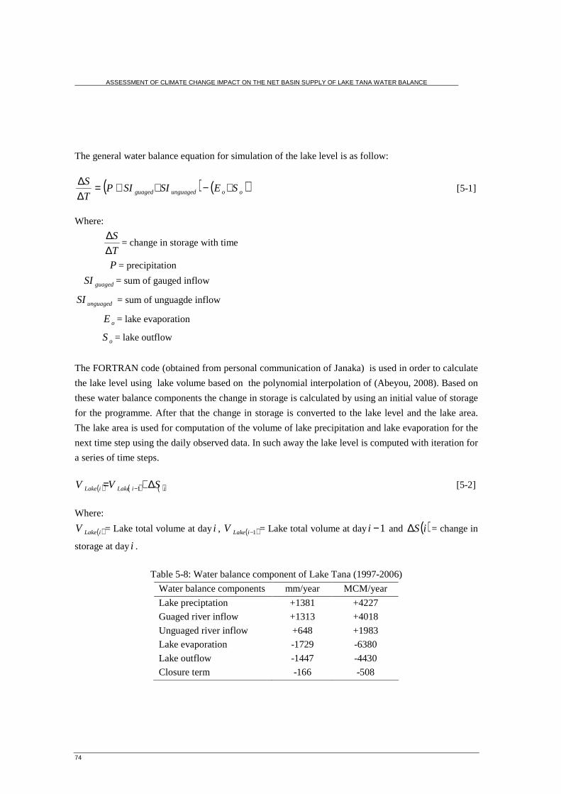
ASSESSMENT OF CLIMATE CHANGE IMPACT ON THE NET BASIN SUPPLY OF LAKE TANA WATER BALANCE
74
The general water balance equation for simulation of the lake level is as follow:
( ) ( )oounguagedguaged SESISIPT
S +−++=∆∆
[5-1]
Where:
T
S
∆∆
= change in storage with time
P = precipitation
guagedSI = sum of gauged inflow
unguagedSI = sum of unguagde inflow
oE = lake evaporation
oS = lake outflow
The FORTRAN code (obtained from personal communication of Janaka) is used in order to calculate
the lake level using lake volume based on the polynomial interpolation of (Abeyou, 2008). Based on
these water balance components the change in storage is calculated by using an initial value of storage
for the programme. After that the change in storage is converted to the lake level and the lake area.
The lake area is used for computation of the volume of lake precipitation and lake evaporation for the
next time step using the daily observed data. In such away the lake level is computed with iteration for
a series of time steps.
( ) ( ) ( )iiLakeiLake SVV ∆+= −1 [5-2]
Where:
( )iLakeV = Lake total volume at dayi , ( )1−iLakeV = Lake total volume at day 1−i and ( )iS∆ = change in
storage at dayi .
Table 5-8: Water balance component of Lake Tana (1997-2006)
Water balance components mm/year MCM/year
Lake preciptation +1381 +4227
Guaged river inflow +1313 +4018
Unguaged river inflow +648 +1983
Lake evaporation -1729 -6380
Lake outflow -1447 -4430
Closure term -166 -508

ASSESSMENT OF CLIMATE CHANGE IMPACT ON THE NET BASIN SUPPLY OF LAKE TANA WATER BALANCE
75
1782
1783
1784
1785
1786
1787
1788
1789
Jan-
97
Jul-9
7
Jan-
98
Jul-9
8
Jan-
99
Jul-9
9
Jan-
00
Jul-0
0
Jan-
01
Jul-0
1
Jan-
02
Jul-0
2
Jan-
03
Jul-0
3
Jan-
04
Jul-0
4
Jan-
05
Jul-0
5
Jan-
06
Jul-0
6
Date
Lake
leve
l (m
)
simulated
observed
Figure 5-47: Simulation of Lake Tana water level (1997-2006)
The closure term indicates the water balance error is 5 % and the relative volume error of 1 %. The
Nash-Sutcliffe coefficient is 0.70.
Table 5-9: Water balance components of (Abeyou, 2008), (Gieske et.al , 2008) and (SMEC, 2007)
Wale (2008) Gieske et.al (2008) SMEC (2007)
Water balance terms mm MCM mm MCM mm MCM
Lake areal rainfall 1220 3784 1255 3891 1260 3906
Guaged river inflow 1280 3970 1297 4021 1622 5028
Unguaged river inflow 880 2729 473 1466 nd nd
Lake evaporation -1690 -5242 -1671 -5180 -1650 -5115
Outflow -1520 -4714 -1348 -4179 -1231 -3813
Closure term -170 -527 6 19 1 3
5.8. Uncertainty and sensitivity analysis
The HadCM3A2a and HadCM3B2a scenarios are the most widely used GCM in climate change
impact studies. The temporal resolution of both models is monthly but hydrological models for
forecasting of the future inflow to the lake requires daily precipitation and temperature. Therefore
computation of the difference between the current and the future climate data and addition of this
change to the 30 years daily data is the most widely used method. This technique is one of the sources
of uncertainty because it assumes that the same anomalies persist every year, which might smooth
inter annual variability of climate variables.

ASSESSMENT OF CLIMATE CHANGE IMPACT ON THE NET BASIN SUPPLY OF LAKE TANA WATER BALANCE
76
The other source of uncertainty in climate change impact assessment is the emission scenarios. For
this study two emission scenarios (A2 and B2) are used. The CO2 concentration for both scenarios in
1990 is 354 parts per million (ppm) but in 2050s the concentration increases to 536 ppm and 478 ppm
with A2 and B2 emission scenarios respectively. But temperature increase as a result of increase in
CO2 concentration for both scenarios is 1.4 oC compared to the 1990 temperature. There are also other
emission scenarios with the same emission of carbon dioxide concentration produces different climate
change scenarios.
In addition to the climate change scenarios synthetic scenarios is used for this study to determine the
sensitivity of the climate variables for the net basin supply of Lake Tana water balance. This scenario
is based on the increasing of the baseline temperature and the precipitation by an arbitrary but
reasonable amount to check the sensitivity of the net basin supply for the climate variables.
Table 5-10: Change of Annual average net basin supply with incremental scenario
Scenario number S-1 S-2 S-3 S-4 S-5 S-6 S-7 S-8 S-9 S-10 S-11
Change in
Precipitation (%) 0 0
0 -10 10 -20 20 -10 10 -20 20
Change in
Temperature ( oC) 1 2
3 1 1 1 1 2 2 2 2
Change in
Evaporation (%) 2.7 5.4
8.2 2.7 2.7 2.7 2.7 5.4 5.4 5.4 5.4
Change of net
basin supply (%) -7.4 -15
-21 -39 44.6 -69 59 -45 17 -75 33
The sensitivity analysis result indicates that an increase in 1oC in temperature reduces the annual
average net basin supply by 7.4 % but the increase in 1oC and a reduction of precipitation by 10 %
reduces the average net basin supply by 38.7%. In the same way the percentage change in
precipitation in the whole scenario shows significant changes to the average annual net basin supply
as compared to the change in temperature. This indicates that net basin supply for Lake Tana is more
sensitive to precipitation than temperature.

ASSESSMENT OF CLIMATE CHANGE IMPACT ON THE NET BASIN SUPPLY OF LAKE TANA WATER BALANCE
77
-30
-25
-20
-15
-10
-5
0
0 1 2 3 4 5
Increase in temperature ( oC)
Cha
nge
of n
et b
asin
sup
ply
(%)
0
2
4
6
8
10
12
Cha
nge
of e
vapo
ratio
n (%
)
net basin supply evaporation Linear (evaporation) Linear (net basin supply)
Figure 5-48: Annual average change of net basin supply and evaporation for change of temperature
-80
-60
-40
-20
0
20
40
60
80
-25 -15 -5 5 15 25
change in precipitation (%)
chan
ge in
net
bas
in s
uppl
y (%
)
Figure 5-49: Annual average change of net basin supply for change of precipitation.
As it is indicated in Figure 5-48 and Figure 5-49 the decrease of precipitation by 10 % and 20 %
reduces the annual mean net basin supply by 32 % and 62 % respectively and the same percentage
increase in precipitation results increases of the net basin supply by 32 % and 62 %. The increase in
temperature by 1, 2 and 3 oC decreases the mean annual net basin supply by 7, 15 and 21 %
respectively. This shows the change in precipitation is more sensitive than change in temperature for
annual average net basin supply. The change in temperature also causes the change in evaporation.
Therefore the sensitivity analysis is made for the mean annual evaporation of Bahir Dar and Gonder
station due to increase in temperature from the baseline period. The sensitivity result indicates an
increase of 1oC, 2 oC, 3 oC and 4 oC for the both maximum and minimum temperature results the
increases of the evaporation by 2.7%, 5.4%, 8.2% and 10.9 % respectively.

ASSESSMENT OF CLIMATE CHANGE IMPACT ON THE NET BASIN SUPPLY OF LAKE TANA WATER BALANCE
78

ASSESSMENT OF CLIMATE CHANGE IMPACT ON THE NET BASIN SUPPLY OF LAKE TANA WATER BALANCE
79
6. Conclusions and Recommendations
6.1. Conclusions
The objective of this study is the assessment of climate change impact on the net basin supply of Lake
Tana water balance. Therefore downscaling of large scale climate variables from GCM outputs to
local scale or regional scale is very essential in order to investigate the hydrological impact of future
climate change scenarios. For this study regression based statistical downscaling methods which
correlate the predictors (regional climate variables) and the predictand (local scale climate variable)
with multiple linear regression equation is applied. The precipitation and temperature data of Bahir
Dar, Gonder and Debre Markos is used for downscaling.
The study confirmed that the statistical downscaling model is able to simulate all climatic variables.
The model simulates the maximum temperature and minimum temperature more accurately than
precipitation. However all simulated climatic variables follow the same trend with the observed one.
The lower performance of the precipitation simulation is based on its nature of being a conditional
process.
The result of the downscaling models indicates that the mean monthly maximum temperature is
increasing by 0.5, 1 and 1.5 oC in 2020s, 2040s and 2070s respectively for HadCM3B2a scenario out
put. For HadCM3A2a scenario output the maximum temperature also increases by 0.52, 1.2 and 2.1oC
in 2020s, 2040s and 2070s respectively compared to the base line period (1961-1990). The increase in
mean monthly minimum temperature 0.66, 1.13 and 1.75 oC for the HadCM3B2a scenario and for
HadCM3A2a scenario the increase is 0.65, 1.4 and 2.35oC in 2020s, 2040s and 2070s respectively. As
a result of increase in maximum and minimum temperature the lake evaporation also increases as
compared to the baseline period. The lake evaporation based on the HadCM3A2a scenario output
indicates that the mean annual evaporation is 1685, 1706 and 1741 mm in the period of 2020s, 2040s
and 2070s respectively. The lake evaporation based on the baseline climate variable is 1674 mm/year.
The downscaled result of precipitation indicates that the mean monthly precipitation is increases by
15.5, 17.8 and 17.4 % for HadCM3B2a scenario output in 2020s, 2040s and 2070s respectively. For
HadCM3A2a scenario output the increase in precipitation is 13.6, 18.5 and 24.8 % in 2002s, 2040s
and 2070s respectively. This increase in precipitation in the future causes for increasing in lake
precipitation and inflow to Lake Tana. The analysis made on the mean annual lake precipitation
indicates that the lake precipitation is 1425mm, 1444 mm and 1540 mm/year for the HadCM3B2a
scenario output in 2020s, 2040s and 2070s and this increase in precipitation for HadCM3A2a scenario
output is 1360 mm, 1361 mm and 1386 mm in the same periods. The lake precipitation in the base
line period is 1312 mm/year.
The ultimate objective of the study is the assessment of climate change impact on the net basin supply
of the Lake Tana water balance. Then a hydrological model is required in order to forecast the inflow

ASSESSMENT OF CLIMATE CHANGE IMPACT ON THE NET BASIN SUPPLY OF LAKE TANA WATER BALANCE
80
to the lake based on the downscaled climate variables. For this the HBV-96 is selected because the
model is tested by many countries for climate change impact studies, it is applicable for different
geographical and climatological regions and it is easily available.
The hydrological analysis indicates that the mean annual inflow to the lake is 1878mm, 1848mm and
1866 mm for the HadCM3B2a scenario and 2062 mm, 2045 mm and 2192 mm with HadCM3A2a
scenario in 2020s, 2040s and 2070s respectively. The mean annual inflow for the baseline period is
1821mm/year. The inflow estimated by HadCM3B2a scenario output is less compared to the
HadCM3A2a scenario outputs. This is because the downscaled precipitation by HadCM3B2a scenario
for all the station is less than the precipitation downscaled by the HadCM3A2a scenario.
The net basin supply in the future time is computed based on the lake evaporation, the lake
precipitation and the inflow to the lake. Even though all component of the net basin supply shows an
increasing trend, the lake evaporation is obscured by the increase in inflow and lake precipitation. The
mean annual net basin supply of Lake Tana based on the HadCM3A2a scenario output is 1801mm,
1783 mm and 1991 mm in 2020s ,2040s and 2070s respectively while the net basin supply within
these successive periods for HadCM3B2a scenario output is 1554, 1481 and 1530. For the baseline
period the mean annual net basin supply is 1459 mm.
The water balance estimation of the Lake (1997-2006) indicates that the mean annual lake
precipitation is 1381 mm, gauged inflow is 1313 mm, unguaged inflow is 648 mm, lake evaporation is
1729mm and outflow is 1447 mm. The contribution of the unguaged inflow is 37 % of the total
inflow discharge to the lake. In Lake Tana the operation of the weir to deliver water to the
hydropower project is begin in 2002. Then it is difficult to observe the impact of climate change on
the outflow and lake level after this period because the water balance components are influenced by
supply to the hydropower plant. But the outflow of Lake Tana was the lowest record in 1984 before
the weir construction. At that time the precipitation of the Lake Tana catchment is decline due the
climate change impact.
The sensitivity analysis made with the incremental scenario method indicates that the net basin supply
of Lake Tana is sensitive to climate change impact. The increase in temperature by 1oC and 2oC
reduce the net basin supply by 7.4 % and 15 % from the baseline period net basin supply while the
decrease in precipitation by 10 % and 20 % reduces the net basin supply by 32 % and 62 % from the
baseline net basin supply. The sensitivity analysis made for evaporation indicates that the increase of
temperature by 1 oC , 2 oC , 3 oC , and 4 oC increase the evaporation by 2.7%, 5.4%, 8.2% and 10.9 %
respectively. Generally the sensitivity result indicates that the net basin supply is more sensitive to
precipitation change than change in temperature.

ASSESSMENT OF CLIMATE CHANGE IMPACT ON THE NET BASIN SUPPLY OF LAKE TANA WATER BALANCE
81
6.2. Recommendations
The GCM outputs, the emission scenarios and the downscaling methods used for this study have
certain level of uncertainty. Therefore further studies should reduce the uncertainty by the use of
different GCM outputs, downscaling methods and emission scenarios. The use of several general
circulation models for climate change studies able to get the better result. Further downscaling
methods especially improves the simulation of the precipitation result is very essential. In this study
only two emission scenarios are applied but in the actual case all SRES emission scenarios have equal
probability of occurrence, then the future study should also consider the entire range of possible
emission scenarios.
For downscaling of climate variables with statistical downscaling model only maximum temperature,
minimum temperature and rainfall data of Bahir Dar, Gonder and Debre Markos stations are applied.
But these stations are not sufficient for downscaling of the entire Lake Tana basin. Therefore further
studies should consider other stations data. Besides, this study can be extended by considering change
in land used, soil type and other climate variables in addition to the change in precipitation and
temperature.

ASSESSMENT OF CLIMATE CHANGE IMPACT ON THE NET BASIN SUPPLY OF LAKE TANA WATER BALANCE
82

ASSESSMENT OF CLIMATE CHANGE IMPACT ON THE NET BASIN SUPPLY OF LAKE TANA WATER BALANCE
83
References:
Abdo Kedir, S., 2008. Assessment of climate change impacts on the hydrology of Gilgel Abbay catchment in Lake Tana basin, Ethiopia, ITC, Enschede, 72 pp.
Abeyou, W., 2008. Hydrological balance of Lake Tana upper Blue Nile basin, Ethiopia, ITC, Enschede, 94 pp.
Allen, R.G., Pereria, L.S., Rase, D. and Smith, M., 1998. Crop Evaporanspiration: FAO Irrigation and Drainage Paper No.56 326pp.
Bergström, S. and Graham, L.P., 1998. On the scale problem in hydrological modeling. Journal of Hydrology, 211(1-4): 253-265.
Booij, M.J., 2005. Impact of climate change on river flooding assessed with different spatial model resolutions. Journal of Hydrology, 303(1-4): 176-198.
Carter, T.R.,2007. General guide lines on the use of scenario data for climate impact and adaptation assessment. Finnish Environmental Institute, Helsinki, Finland.
Clair , E. Hanson, Tom Holt and Jean P Paluikof, February 2004. An Integrated Assessment of the potential for change in storm activity over Europe: Implications for insurance and forestry in the UK .Tyndall centre for climate change research technical report12, 10-11pp.
Conway, D., 2000. The Climate and Hydrology of the Upper Blue Nile River. The Geographical Journal, 166: 49-62.
Das, T., Bárdossy, A., Zehe, E. and He, Y., 2008. Comparison of conceptual model performance using different representations of spatial variability. Journal of Hydrology, 356(1-2): 106-118.
Dawson, C.W. & Wilbey, R.L., 2007. Statistical Downscaling Model, version 4.2. Department of Geography , Lancaster University, UK.
deBoer, B., 2007. Climate change and impacts on the extreme rainfall over the Blue Nile region. KNMI, Royal Netherlands Meteorological Institute, De Bilt, Netherlands.
Dibike, Y.B. and Coulibaly, P., 2005. Hydrologic impact of climate change in the Saguenay watershed: comparison of downscaling methods and hydrologic models. Journal of Hydrology, 307(1-4): 145-163.
Gieske, Abeyou, W., Getachew, HA., Alemseged TH., Rientjes, T.H.M, 2008. Non-linear parameterization of Lake Tana flow system.Hydrology and ecology of Nile River Basin under extreme conditions, Wossenu Abtew, Assefa M. Melesse (eds). Proceeding of the workshop, Addis ababa, 2008; 128-145.
Goodess, C.M., Osborn, C.T., Hulme, M. and Tyndall Centre for Climate Change, R., 2003. The Identification and Evaluation of Suitable Scenario Development Methods for the Estimation of Future Probabilities of Extreme Weather Events. Tyndall Centre for Climate Change Research.

ASSESSMENT OF CLIMATE CHANGE IMPACT ON THE NET BASIN SUPPLY OF LAKE TANA WATER BALANCE
84
Hay, L.E. and Clarck, M.P., 2003. Use of statistically and dynamically downscaled atmospheric model output for hydrologic simulations in three mountainous basins in the western United States. Journal of Hydrology , 282 (1-4) : 56-75.
Kaba Ayana, E., 2007. Validation of radar altimetry lake level data and it's application in water resource management, ITC, Enschede, 76 pp.
Kebede, S., Travi, Y., Alemayehu, T. and Marc, V., 2006. Water balance of Lake Tana and its sensitivity to fluctuations in rainfall, Blue Nile basin, Ethiopia. Journal of Hydrology, 316(1-4): 233-247.
Krysanova, V., Bronstert, A. and Müller-Wohlfeil, D.-I., 1999. Modelling river discharge for large drainage basins: from lumped to distributed approach. Hydrological Sciences Journal, 44: 313-331
Luis, A.J. and Pandey, P.C., 2005. Characteristics of atmospheric divergence and convergence in the Indian Ocean inferred from scatterometer winds. Remote Sensing of Environment, 97(2): 231-237.
Maidment, D.R., 1993. Handbook of Hydrology, McGraw-Hill.
Menzel, L. and Bürger, G., 2002. Climate change scenarios and runoff response in the Mulde catchment (Southern Elbe, Germany). Journal of Hydrology, 267(1-2): 53-64.
Mujumdar, P.P., 2008. Implications of climate change for sustainable water resources management in India. Physics and Chemistry of the Earth, Parts A/B/C, 33(5): 354-358.
Palmer, Richard N., Erin Clancy , Nathan T. Van Rheenen, and Mattew W.Wiley, 2004. The impacts of climate change on the Tualatine River basin water supply: An investigation into projected hydrologic and management impacts. Department of civil and environmental engineering, University of Washington, 67pp.
Rientjes, T.H.M., 2007. Modelling in hydrology. Department of water resources, ITC, Enschede.
Seibert, J., 2002. HBV light: version 2 User's Manual. Department of Earth Science, Hydrology, Uppsala University, Sweden.
SMHI, 2006. Integrated Hydrological Modelling System Manual, Version 5.1.
SMEC International Pty Ltd, 2007. Hydrological Study of the Tana-Beles Subbasins Interim Report, Snowy Mountain Engineering Corporation, Australia, 77pp.
Ungtea Kim and Jagath Kaluarachchi., 2008. Analysis of hydrology and water resources of the Upper Blue Nile river basin under climate change. Hydrology and Ecology of the Nile river basin under extreme conditions, Wossenu Abtew, Assefa M. Melesee (eds). Proceeding of the workshop, Addis ababa, 2008; 15-34.
Vallet-Coulomb, C., Legesse, D., Gasse, F., Travi, Y. and Chernet, T., 2001. Lake evaporation estimates in tropical Africa (Lake Ziway, Ethiopia). Journal of Hydrology, 245(1-4): 1-18.
Wilby, R. et al., 2004. Guidelines for use of climate scenarios developed from statistical downscaling methods. IPCC Data Distribution Centre Report, UEA, Norwich, UK, 27.

ASSESSMENT OF CLIMATE CHANGE IMPACT ON THE NET BASIN SUPPLY OF LAKE TANA WATER BALANCE
85
Annexes:
Appendix A : Catchment extraction procedures

ASSESSMENT OF CLIMATE CHANGE IMPACT ON THE NET BASIN SUPPLY OF LAKE TANA WATER BALANCE
86
Appendix B: Hydrological and meteorological station and their location
Hydrological stations and their locations
Meteorological stations and their location
River Guaging station Latitude (utm) Longitude (utm) outlet elevation
(m amsl )
Gilgel Abbay Near Merawi 285380.315 1257135.310 1889
Koga At Merawi 287199.781 1257123.048 1898
Kelti Nera Delgi 276374.243 1270104.996 1876
Ribb Near Addis
Zemen
360283.969 1326759.723 1796
Gumara Near Bahir Dar 351119.160 1308370.538 1794
Megech Near Azezo 331552.842 1380369.401 1865
Gemero Near Maksegnit 342362.313 1369247.425 1879
Garno Near Enfranze 349525.939 1352618.885 1856
Gelda Near Ambesame 351605.015 1404223.536 2036
Staions Longitude (utm) Latitude (utm) Elevation (m amsl)
Addis zemen 1376576.884 376576.884 2117
Debre Tabour 1309918.026 401873.898 2714
Gondar 1387682.311 327881.649 2074
Bahir Dar 1282605.753 325456.442 1828
Dangila 1245380.969 265187.251 2126
Sekella 1216350.924 305057.004 2584
Enjibara 1212886.813 270418.731 2580
Gundil 1210918.62 288991.214 2546
Adet 1245695.593 332531.137 2230
Kidamaja 1216653.109 259512.914 2456
Abbay Sheleko 1259013.797 267107.339 2000
Enfranze 1346966.733 356659.457 1889

ASSESSMENT OF CLIMATE CHANGE IMPACT ON THE NET BASIN SUPPLY OF LAKE TANA WATER BALANCE
87
Appendix C: Catchment characteristics of unguaged catchment
Sub catchment Area Hypsometric
Integral
Average
Slope %
%
Level
%
Hilly
%
Steepy
Average
Elevation
(m amsl)
Gelda 356.1 0.48 17.91 69.64 29.23 1.13 2116
Unguaged Gumara 517.3 0.39 17.29 79.04 20.28 0.69 2010
Unguaged Ribb 711.5 0.46 35.19 64.29 27.15 8.56 2421
UnguagedMegechh 462.3 0.43 18.03 76.72 22.30 0.98 2237
Unguaged
Gilgelabbay
1991 0.45 19.93 89.83 9.21 1.93 2186
Garno 256.5 0.46 37.65 28.89 41.03 30.08 2337
Gumero 389.9 0.5 34.04 52.56 31.13 16.3 2313
Derma 376 0.48 16.6 72.78 26.46 0.76 2144
Gabikura 382.5 0.49 14.53 84.18 15.45 0.37 2002
Tana west 610.6 0.49 20.91 59.87 38.11 2.02 2038
Sub
catchment
% of
Leptosols
% of
Nitisols
% of
Luvisols
% of
Vertisols
% of
Fluvisols
Elongation
Ratio
Length of longest
flow path
Gelda 0.74 0.00 96.74 2.52 0.00 1.88 42.42
Unguaged
Gumara
0.30 0.00 50.32 26.82 22.56 0.60 14.83
Unguaged
Ribb
28.56 0.56 9.08 14.46 47.35 0.58 17.53
Unguaged
G.Abbay
22.5 4.5 54.38 13.27 4.9 2.04 76.96
Ungauged
Megech
17.48 0.00 12.40 50.09 20.0 1.42 34.93
Garno 59.51 6.64 2.95 21.53 9.37 1.73 37.03
Gumero 42.33 2.04 13.68 41.12 0.83 1.67 44.12
Derma 23.39 0.00 5.11 69.39 2.11 2.07 45.38
Gabi Kura 1.32 0.00 11.87 69.04 17.78 1.44 31.54
Tana west 0.10 0.00 39.21 2.79 57.89 0.72 20.34

ASSESSMENT OF CLIMATE CHANGE IMPACT ON THE NET BASIN SUPPLY OF LAKE TANA WATER BALANCE
88
Appendix D: Correlation coefficient between model parameters and catchment characteristics.
Alfa= 1.65-0.26 *Percentage of bare land -0.02*Percentage of hilly [1]
Beta =1.17+0.000808*Catchment area-0.014*Percentage of hilly [2]
FC=2142.81-0.803*Catchment area -17.33*Percentage of hilly [3]
K4=0.049-0.057*Hypsometric integral-o.001*Percentage of nitsols [4]
-0.001*Percentage of Fluvisols
Perc=-0.23 +0.36*log (Percentage of Luvisols) [5]
-0.114*log (Percentage of Bare Land)
KHQ=0.113-0.000036*Catchment area +0.000602*Percentage of luvisols [6]
LP=0.06+0.0006*Catchment area -0.12*Percentage of bare land [7]
Hq=4.64+0.0019*Catchment area -2.34 *Percentage of bare land [8]
NB.The unit of the catchment area is in Km2

ASSESSMENT OF CLIMATE CHANGE IMPACT ON THE NET BASIN SUPPLY OF LAKE TANA WATER BALANCE
89
Appendix E: Double mass curve for some of gauged catchments and Rainfall
Stations.
Double mass curve is the hydrological method used to analyse the consistence of precipitation and
discharge. To check the consistency of the discharge data the cumulative daily rainfall with the
cumulative daily discharge of Megech, Ribb, Gilgel Abbay, and Gumara are made in the excel. Beside
this the cumulative daily rainfall of 10 stations are made with the cumulative rainfall of Bahir Dar
station. Bahir Dar station is taken as the base station since it has long time series data and it is
reliable.
In double mass analysis the cumulative rainfall is directly related the cumulative discharge. During
the dry season the cumulative rainfall is almost constant since the daily rainfall is almost negligible.
As a result the cumulative discharge could not show an increasing trend. If an increment of discharge
with out rainfall distribution there may be a problem in the discharge record at that period. In same
way there must be an increasing trend in the main wet season due to increasing rainfall. Generally by
observing the trend of the cumulative rainfall and cumulative discharge it is possible to identify the
problem in the discharge record.
The double mass curve between the base station (Bahir Dar) and other rainfall stations is used to
identify the homoginty of the records between each other. Even tough the spatial distribution of the
rainfall is different; the cumulative rainfall between the stations could not show an abrupt change.
During the dry seasons both the base station and the other station records less amount of rainfall then
the slope of the plot become almost zero. But in rainy seasons there is considerable amount of rainfall
in both stations then the slope the plot become positive. With visual interpretation of the plot it is
possible to identify where the error in rainfall record.
Gilgel Abbay
0
50000
100000
150000
200000
250000
0 5000 10000 15000 20000 25000
Cumulative rainfall (mm/day)
Cu
mu
lati
ve d
isch
arg
e (m
3/s)
Gumara
0
20000
40000
60000
80000
100000
120000
140000
0 2000 4000 6000 8000 10000 12000 14000 16000
Cummulative rainfall (mm/day)
Cu
mm
ula
tive
dis
chra
ge(
m3 /s
)

ASSESSMENT OF CLIMATE CHANGE IMPACT ON THE NET BASIN SUPPLY OF LAKE TANA WATER BALANCE
90
0
500
1000
1500
2000
2500
3000
3500
4000
0 1000 2000 3000 4000 5000
Bahirdar cummulative rainfall (mm/day)
Ab
ay s
hel
eko
cu
mm
ula
tive
ra
infa
ll (m
m/d
ay)
0
500
1000
1500
2000
2500
3000
3500
4000
0 1000 2000 3000 4000
Bahirdar cummulative rainfall (mm/day)
Sek
ela
cum
mu
lati
ve r
ain
fall
(mm
/day
)
Megech
0
5000
10000
15000
20000
25000
30000
35000
0 2000 4000 6000 8000 10000 12000
Cummulative rainfall (mm/day)
cum
mu
lati
ve d
isch
arg
e (m
3 /s)
Ribb
0
10000
20000
30000
40000
50000
60000
0 5000 10000 15000 20000
Cummulative rainfall (mm/day)
Cu
mm
ula
tive
d
isch
arg
e(m
3 /s)
0
1000
2000
3000
4000
5000
6000
7000
8000
0 1000 2000 3000 4000 5000
Bahirdar cummulative rainfall (mm/day)
En
gib
ara
cum
mu
lati
ve r
ain
fall
(mm
/day
)
0
500
1000
1500
2000
2500
3000
3500
0 1000 2000 3000 4000 5000
Bahirdarcummulative rainfall (mm/day)
En
fran
ze c
um
mu
lati
ve r
ain
fall
(mm
/day
)

ASSESSMENT OF CLIMATE CHANGE IMPACT ON THE NET BASIN SUPPLY OF LAKE TANA WATER BALANCE
91
0
500
1000
1500
2000
2500
3000
3500
4000
4500
5000
0 1000 2000 3000 4000 5000
Bahirdar cummulative rainfall (mm/day)
Deb
reta
bo
ur
cum
mu
lati
ve r
ain
fall
(mm
/day
)
0
500
1000
1500
2000
2500
3000
3500
4000
4500
0 1000 2000 3000 4000 5000
Bahirdarcumulative rainfall (mm/day)
Ad
et c
um
mu
lati
ve r
ain
fall
(mm
/day
)
0
1000
2000
3000
4000
5000
6000
0 1000 2000 3000 4000 5000
Bahirdarcummulative rainfall (mm/day)
Dan
gila
cu
mm
ula
tive
rai
nfa
ll (m
m/d
ay)
0
500
1000
1500
2000
2500
3000
3500
4000
4500
0 1000 2000 3000 4000 5000
Bahirdar cummulative rainfall (mm/day)
Deb
rem
arko
s cu
mm
ula
tive
rai
nfa
ll (m
m/d
ay)
0.00
1000.00
2000.00
3000.00
4000.00
5000.00
6000.00
7000.00
0 1000 2000 3000 4000 5000
Bahirdar cummulative rainfall (mm/day)
Kid
amaj
a cu
mm
ula
tive
rai
nfa
ll (m
m/d
ay)
0
1000
2000
3000
4000
5000
6000
7000
8000
0 1000 2000 3000 4000 5000
Bahirdar cummulative rainfall (mm/day)
Gu
nd
il cu
mm
ula
tive
rai
nfa
ll (m
m/d
ay)

ASSESSMENT OF CLIMATE CHANGE IMPACT ON THE NET BASIN SUPPLY OF LAKE TANA WATER BALANCE
92
Appendix F: Downscaled maximum temperature, minimum temperature and rainfall
Maximum temperature change with HadCM3A2a scenario output of Debre Markos station
Monthly average
maximum temperature (oC)
Temperature change
compared to the 1961-1990 (oC)
Months 1961-
1990
1991-
2006
2010-
2039
2040-
2069
2070-
2099
1991-
2006
2010-
2039
2040-
2069
2070-
2099
January 24.41 24.04 24.88 25.40 26.15 -0.37 0.47 0.99 1.74
February 24.66 23.18 24.98 25.47 25.99 -1.48 0.32 0.81 1.33
March 25.05 25.74 25.54 26.01 27.07 0.69 0.49 0.96 2.02
April 25.06 24.42 25.38 25.69 26.22 -0.64 0.32 0.63 1.16
May 23.35 24.45 24.30 25.18 26.62 1.1 0.95 1.83 3.27
June 21.34 20.30 22.81 24.14 26.30 -1.04 1.47 2.80 4.96
July 19.14 18.88 19.56 19.99 20.64 -0.26 0.42 0.85 1.50
August 19.10 18.94 19.38 19.75 20.32 -0.16 0.28 0.65 1.22
September 19.73 19.87 20.01 20.27 20.58 0.14 0.28 0.54 0.85
October 21.33 21.82 21.91 22.50 23.23 0.49 0.58 1.17 1.90
November 22.04 22.11 22.50 23.04 23.79 0.08 0.46 1.00 1.75
December 22.60 23.45 23.02 23.62 24.27 0.85 0.42 1.02 1.67
Maximum temperature change with HadCM3B2a scenario output of Debre Markos
Monthly average
Maximum temperature ( oC)
Temperature change
compared to 1961-1990 ( oC)
Months 1961-
1990
1991-
2006
2010-
2039
2040-
2069
2070-
2099
1991-
2006
2010-
2039
2040-
2069
2070-
2099
January 24.41 24.04 24.88 25.40 26.15 -0.37 0.48 0.99 1.74
February 24.66 23.18 24.98 25.47 25.99 -1.48 0.32 0.80 1.33
March 25.05 25.74 25.54 26.01 27.07 0.69 0.49 0.96 2.02
April 25.06 24.42 25.38 25.69 26.22 -0.64 0.32 0.63 1.16
May 23.35 24.45 24.30 25.18 26.62 1.10 0.94 1.83 3.27
June 21.34 20.30 22.81 24.14 26.30 -1.04 1.47 2.80 4.96
July 19.14 18.88 19.56 19.99 20.64 -0.26 0.42 0.85 1.50
August 19.10 18.94 19.38 19.75 20.32 -0.16 0.28 0.64 1.21
September 19.73 19.87 20.01 20.27 20.58 0.14 0.28 0.54 0.85
October 21.33 21.82 21.91 22.50 23.23 0.49 0.57 1.17 1.90
November 22.04 22.11 22.50 23.04 23.79 0.08 0.47 1.01 1.75
December 22.60 23.45 23.02 23.62 24.27 0.85 0.42 1.01 1.67

ASSESSMENT OF CLIMATE CHANGE IMPACT ON THE NET BASIN SUPPLY OF LAKE TANA WATER BALANCE
93
Minimum temperature change with HadCM3B2a scenario output of Debre Markos station
Monthly average
Minimum temperature ( oC)
Temperature change
compared to 1961-1990 ( oC)
Months 1961-
1990
1991-
2006
2010-
2039
2040-
2069
2070-
2099
1991-
2006
2010-
2039
2040-
2069
2070-
2099
January 7.30 9.15 8.09 8.56 9.35 1.85 0.79 1.27 2.05
February 8.85 9.38 9.44 9.87 10.50 0.54 0.59 1.02 1.66
March 10.21 11.36 10.98 11.55 12.39 1.15 0.77 1.34 2.18
April 10.89 11.78 11.96 12.80 14.06 0.89 1.06 1.91 3.17
May 10.62 11.90 11.25 11.71 12.35 1.28 0.63 1.09 1.73
June 9.81 10.53 10.27 10.59 10.99 0.72 0.46 0.78 1.18
July 10.05 11.03 10.34 10.54 10.79 0.97 0.28 0.49 0.73
August 9.77 10.99 10.07 10.29 10.63 1.22 0.30 0.52 0.86
September 9.36 9.91 10.18 10.70 11.52 0.56 0.82 1.34 2.16
October 8.89 9.91 9.50 9.84 10.33 1.02 0.61 0.94 1.44
November 7.49 8.70 8.38 8.90 9.62 1.21 0.89 1.41 2.13
December 6.83 8.67 7.66 8.38 9.27 1.84 0.83 1.55 2.44
Minimum temperature change with HadCM3A2a scenario out put of Debre Markos station.
Monthly average
Minimum temperature ( oC)
Temperature change
compared to 1961-1990 (oC)
Months 1961-
1990
1991-
2006
2010-
2039
2040-
2069
2070-
2099
1991-
2006
2010-
2039
2040-
2069
2070-
2099
January 7.30 9.15 8.06 9.01 10.07 1.85 0.77 1.71 2.77
February 8.85 9.38 9.49 10.28 11.18 0.54 0.65 1.44 2.34
March 10.21 11.36 10.94 11.88 13.26 1.15 0.73 1.67 3.05
April 10.89 11.78 12.13 13.32 15.19 0.89 1.24 2.43 4.30
May 10.62 11.90 11.29 11.96 12.97 1.28 0.67 1.34 2.35
June 9.81 10.53 10.28 10.75 11.38 0.72 0.47 0.94 1.57
July 10.05 11.03 10.32 10.62 11.06 0.97 0.27 0.57 1.01
August 9.77 10.99 10.08 10.42 10.89 1.22 0.30 0.65 1.12
September 9.36 9.91 10.14 11.07 12.35 0.56 0.78 1.72 2.99
October 8.89 9.91 9.47 10.08 10.93 1.02 0.57 1.18 2.03
November 7.49 8.70 8.34 9.22 10.52 1.21 0.85 1.73 3.03
December 6.83 8.67 7.70 8.79 10.15 1.84 0.87 1.96 3.33
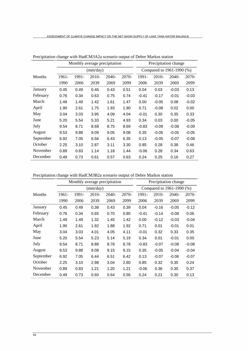
ASSESSMENT OF CLIMATE CHANGE IMPACT ON THE NET BASIN SUPPLY OF LAKE TANA WATER BALANCE
94
Precipitation change with HadCM3A2a scenario output of Debre Markos station
Monthly average precipitation
(mm/day)
Precipitation change
Compared to 1961-1990 (%)
Months 1961-
1990
1991-
2006
2010-
2039
2040-
2069
2070-
2099
1991-
2006
2010-
2039
2040-
2069
2070-
2099
January 0.45 0.49 0.46 0.43 0.51 0.04 0.03 -0.03 0.13
February 0.76 0.34 0.63 0.75 0.74 -0.41 -0.17 -0.01 -0.03
March 1.49 1.49 1.42 1.61 1.47 0.00 -0.05 0.08 -0.02
April 1.90 2.61 1.75 1.93 1.90 0.71 -0.08 0.02 0.00
May 3.04 3.03 3.95 4.09 4.04 -0.01 0.30 0.35 0.33
June 5.20 5.54 5.33 5.21 4.93 0.34 0.03 0.00 -0.05
July 9.54 8.71 8.68 8.75 8.69 -0.83 -0.09 -0.08 -0.09
August 9.53 9.88 9.09 9.05 9.08 0.35 -0.05 -0.05 -0.05
September 6.92 7.05 6.56 6.43 6.35 0.13 -0.05 -0.07 -0.08
October 2.25 3.10 2.87 3.11 3.30 0.85 0.28 0.38 0.46
November 0.89 0.83 1.14 1.18 1.44 -0.06 0.28 0.34 0.63
December 0.49 0.73 0.61 0.57 0.63 0.24 0.25 0.16 0.27
Precipitation change with HadCM3B2a scenario output of Debre Markos station
Monthly average precipitation
(mm/day)
Precipitation change
Compared to 1961-1990 (%)
Months 1961-
1990
1991-
2006
2010-
2039
2040-
2069
2070-
2099
1991-
2006
2010-
2039
2040-
2069
2070-
2099
January 0.45 0.49 0.38 0.43 0.39 0.04 -0.16 -0.05 -0.12
February 0.76 0.34 0.65 0.70 0.80 -0.41 -0.14 -0.08 0.06
March 1.49 1.49 1.32 1.45 1.42 0.00 -0.12 -0.03 -0.04
April 1.90 2.61 1.92 1.88 1.92 0.71 0.01 -0.01 0.01
May 3.04 3.03 4.01 4.05 4.11 -0.01 0.32 0.33 0.35
June 5.20 5.54 5.23 5.14 5.19 0.34 0.01 -0.01 0.00
July 9.54 8.71 8.88 8.78 8.78 -0.83 -0.07 -0.08 -0.08
August 9.53 9.88 9.08 9.15 9.15 0.35 -0.05 -0.04 -0.04
September 6.92 7.05 6.44 6.51 6.42 0.13 -0.07 -0.06 -0.07
October 2.25 3.10 2.98 3.04 2.80 0.85 0.32 0.35 0.24
November 0.89 0.83 1.21 1.20 1.21 -0.06 0.36 0.35 0.37
December 0.49 0.73 0.60 0.64 0.56 0.24 0.21 0.30 0.13

ASSESSMENT OF CLIMATE CHANGE IMPACT ON THE NET BASIN SUPPLY OF LAKE TANA WATER BALANCE
95
Maximum temperature change with HadCM3A2a scenario output of Bahir Dar station
Monthly average
maximum temperature (oC)
Temperature change
compared to 1961-1990 ( oC)
Months 1961-
1990
1991-
2007
2010-
2039
2040-
2069
2070-
2099
1991-
2007
2010-
2039
2040-
2069
2070-
2099
January 26.16 26.75 26.78 27.62 28.48 0.58 0.61 1.46 2.31
February 27.81 28.77 28.27 29.03 29.82 0.95 0.46 1.22 2.01
March 29.51 29.68 29.82 30.24 31.10 0.17 0.31 0.73 1.59
April 29.57 30.09 30.23 30.74 31.62 0.52 0.66 1.17 2.05
May 28.35 29.32 28.77 29.16 29.84 0.97 0.42 0.81 1.49
June 26.42 26.88 27.20 28.02 29.51 0.46 0.79 1.60 3.10
July 23.77 24.29 24.16 24.95 26.25 0.52 0.39 1.18 2.47
August 23.44 24.30 23.98 24.82 26.21 0.85 0.54 1.38 2.77
September 24.70 25.59 24.96 25.52 26.12 0.89 0.27 0.82 1.42
October 26.19 26.55 26.85 27.65 28.76 0.35 0.66 1.46 2.57
November 25.98 26.70 26.56 27.32 28.24 0.71 0.57 1.34 2.25
December 25.76 26.70 26.38 27.17 28.20 0.94 0.62 1.41 2.45
Maximum temperature change with HadCM3B2a scenario output of Bahir Dar station
Monthly average
maximum temperature (oC)
Temperature change
Compared to 1961-1990 (oC)
Months 1961-
1990
1991-
2007
2010-
2039
2040-
2069
2070-
2099
1991-
2007
2010-
2039
2040-
2069
2070-
2099
January 26.16 26.75 26.84 27.24 27.88 0.58 0.67 1.04 1.71
February 27.81 28.77 28.20 28.69 29.14 0.95 0.39 0.94 1.33
March 29.51 29.68 29.80 30.14 30.57 0.17 0.29 0.77 1.06
April 29.57 30.09 30.02 30.51 31.05 0.52 0.45 1.04 1.49
May 28.35 29.32 28.65 29.11 29.46 0.97 0.30 0.81 1.12
June 26.42 26.88 27.29 27.85 28.84 0.46 0.87 1.56 2.43
July 23.77 24.29 24.24 24.77 25.71 0.52 0.47 1.47 1.94
August 23.44 24.30 23.93 24.62 25.35 0.85 0.49 1.42 1.90
September 24.70 25.59 25.06 25.23 25.72 0.89 0.36 0.66 1.02
October 26.19 26.55 26.96 27.44 28.12 0.35 0.77 1.16 1.93
November 25.98 26.70 26.64 27.03 27.61 0.71 0.66 0.97 1.63
December 25.76 26.70 26.34 26.84 27.54 0.94 0.58 1.20 1.78

ASSESSMENT OF CLIMATE CHANGE IMPACT ON THE NET BASIN SUPPLY OF LAKE TANA WATER BALANCE
96
Minimum temperature change with HadCM3A2a scenario output of Bahir Dar station
Monthly average
Minimum temperature (oC)
Temperature change
compared to 1961-1990 (oC)
Months 1961-
1990
1991-
2007
2010-
2039
2040-
2069
2070-
2099
1991-
2007
2010-
2039
2040-
2069
2070-
2099
January 6.52 8.87 7.12 8.12 8.92 2.35 0.60 1.60 2.40
February 8.27 10.88 9.07 10.07 11.67 2.60 0.80 1.80 3.40
March 11.30 13.09 12.70 13.90 15.70 1.79 1.40 2.60 4.40
April 12.51 15.18 14.31 15.91 18.31 2.67 1.80 3.40 5.80
May 13.47 15.50 14.67 15.87 17.27 2.03 1.20 2.40 3.80
June 13.36 14.70 14.76 15.96 17.56 1.34 1.40 2.60 4.20
July 13.24 14.35 13.64 14.44 15.04 1.12 0.40 1.20 1.80
August 13.14 14.16 13.74 14.54 15.24 1.01 0.60 1.40 2.10
September 12.37 13.53 13.57 15.17 16.97 1.16 1.20 2.80 4.60
October 11.91 13.87 12.71 13.71 15.11 1.96 0.80 1.80 3.20
November 9.81 11.79 10.81 12.21 13.41 1.98 1.00 2.40 3.60
December 6.94 9.56 8.34 10.14 12.34 2.62 1.40 3.20 5.40
Minimum temperature change with HadCM3B2a scenario output of Bahir Dar station
Monthly average
Minimum temperature (oC)
Temperature change
compared to 1961-1990 (oC)
Months 1961-
1990
1991-
2007
2010-
2039
2040-
2069
2070-
2099
1991-
2007
2010-
2039
2040-
2069
2070-
2099
January 6.52 8.87 7.09 7.89 8.29 2.35 0.57 1.37 1.77
February 8.27 10.88 9.05 9.85 10.65 2.60 0.78 1.58 2.38
March 11.30 13.09 12.64 13.64 14.64 1.79 1.34 2.34 3.34
April 12.51 15.18 14.00 15.20 16.80 2.67 1.49 2.69 4.29
May 13.47 15.50 14.67 15.27 16.27 2.03 1.20 1.80 2.80
June 13.36 14.70 14.76 15.56 16.56 1.34 1.39 2.19 3.19
July 13.24 14.35 13.86 14.06 14.66 1.12 0.62 0.82 1.42
August 13.14 14.16 13.96 14.36 14.96 1.01 0.82 1.22 1.82
September 12.37 13.53 13.70 14.10 15.70 1.16 1.33 1.73 3.33
October 11.91 13.87 12.67 13.47 14.07 1.96 0.76 1.56 2.16
November 9.81 11.79 10.95 11.55 12.55 1.98 1.14 1.74 2.74
December 6.94 9.56 8.28 9.68 11.08 2.62 1.34 2.74 4.14

ASSESSMENT OF CLIMATE CHANGE IMPACT ON THE NET BASIN SUPPLY OF LAKE TANA WATER BALANCE
97
Precipitation change with HadCM3A2a scenario output of Bahir Dar station
Monthly average
Precipitation (mm/day)
Precipitation change compared to
1961-1990 (%)
Months 1961-
1990
1991-
2007
2010-
2039
2040-
2069
2070-
2099
1991-
2007
2010-
2039
2040-
2069
2070-
2099
January 0.10 0.05 0.11 0.13 0.15 -0.05 0.08 0.32 0.51
February 0.08 0.08 0.09 0.09 0.10 0.00 0.19 0.16 0.28
March 0.22 0.44 0.22 0.24 0.23 0.22 -0.04 0.08 0.03
April 0.73 0.95 0.75 0.84 0.97 0.23 0.03 0.16 0.33
May 2.67 2.42 3.57 3.75 3.85 -0.25 0.34 0.41 0.44
June 5.97 7.28 5.43 5.32 5.26 1.31 -0.09 -0.11 -0.12
July 14.38 13.60 13.90 14.23 13.93 -0.78 -0.03 -0.01 -0.03
August 12.65 11.93 12.31 11.91 11.83 -0.72 -0.03 -0.06 -0.06
September 6.75 6.89 9.10 8.75 9.07 0.14 0.35 0.30 0.34
October 2.89 3.22 5.22 5.78 6.29 0.33 0.80 1.00 1.17
November 0.75 0.43 1.42 1.51 1.63 -0.31 0.90 1.03 1.19
December 0.12 0.09 0.27 0.24 0.29 -0.02 1.31 1.07 1.49
Precipitation change with HadCM3B2a scenario output of Bahir Dar station
Monthly average
Precipitation (mm/day)
Precipitation change
Compared to 1961-1990 (%)
Months 1961-
1990
1991-
2007
2010-
2039
2040-
2069
2070-
2099
1991-
2007
2010-
2039
2040-
2069
2070-
2099
January 0.10 0.05 0.09 0.11 0.09 -0.05 -0.08 0.11 -0.11
February 0.08 0.08 0.08 0.09 0.10 0.00 0.05 0.13 0.22
March 0.22 0.44 0.20 0.23 0.23 0.22 -0.10 0.04 0.01
April 0.73 0.95 0.83 0.85 0.80 0.23 0.14 0.17 0.10
May 2.67 2.42 3.38 3.26 3.43 -0.25 0.27 0.22 0.29
June 5.97 7.28 4.79 4.93 4.53 1.31 -0.20 -0.17 -0.24
July 14.38 13.60 13.36 13.72 13.42 -0.78 -0.07 -0.05 -0.07
August 12.65 11.93 11.25 11.17 10.83 -0.72 -0.11 -0.12 -0.14
September 6.75 6.89 8.20 8.10 8.15 0.14 0.21 0.20 0.21
October 2.89 3.22 5.22 4.81 4.47 0.33 0.80 0.66 0.55
November 0.75 0.43 1.37 1.43 1.38 -0.31 0.84 0.91 0.85
December 0.12 0.09 0.25 0.24 0.24 -0.02 1.12 1.05 1.00

ASSESSMENT OF CLIMATE CHANGE IMPACT ON THE NET BASIN SUPPLY OF LAKE TANA WATER BALANCE
98


