Assessment of endocrine disrupting chemicals in water...

Assessment of endocrine disrupting chemicals

in water and sediment samples from

British Columbia, Canada

by

Farhana Ali

B.Sc. (Honours), Simon Fraser University, 2011

Research Project Submitted in Partial Fulfillment of the

Requirements for the Degree of

Master of Environmental Toxicology

in the

Department of Biological Sciences

Faculty of Science

Farhana Ali 2015

SIMON FRASER UNIVERSITY

Fall 2015

ii

Approval

Name: Farhana Ali

Degree: Master of Environmental Toxicology

Title: Assessment of endocrine disrupting chemicals in water and sediment samples from British Columbia, Canada

Examining Committee: Chair: Dr. Felix Breden Professor

Dr. Francis Law Senior Supervisor Professor

Dr. Margo Moore Supervisor Professor

Dr. Christoper Kennedy Internal Examiner Professor

Date Defended/Approved:

November 25, 2015

iii

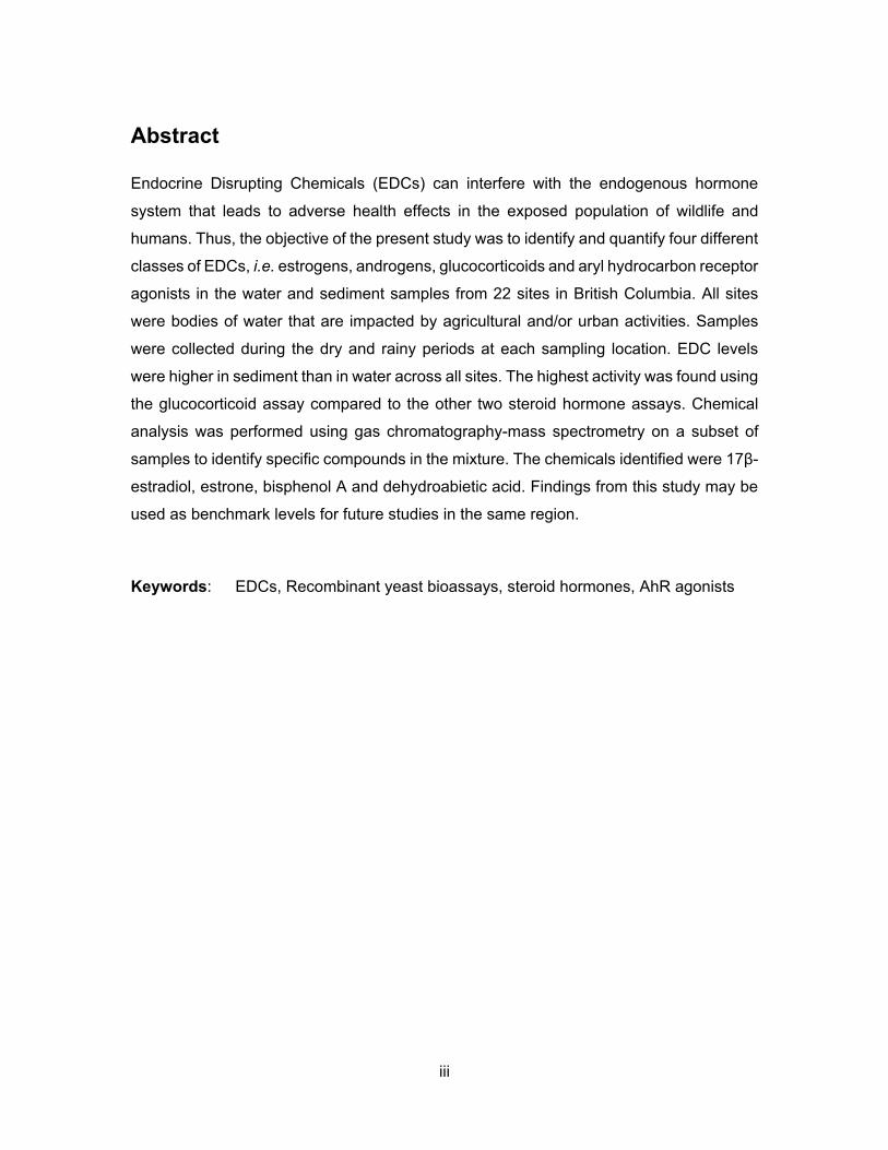
Abstract

Endocrine Disrupting Chemicals (EDCs) can interfere with the endogenous hormone

system that leads to adverse health effects in the exposed population of wildlife and

humans. Thus, the objective of the present study was to identify and quantify four different

classes of EDCs, i.e. estrogens, androgens, glucocorticoids and aryl hydrocarbon receptor

agonists in the water and sediment samples from 22 sites in British Columbia. All sites

were bodies of water that are impacted by agricultural and/or urban activities. Samples

were collected during the dry and rainy periods at each sampling location. EDC levels

were higher in sediment than in water across all sites. The highest activity was found using

the glucocorticoid assay compared to the other two steroid hormone assays. Chemical

analysis was performed using gas chromatography-mass spectrometry on a subset of

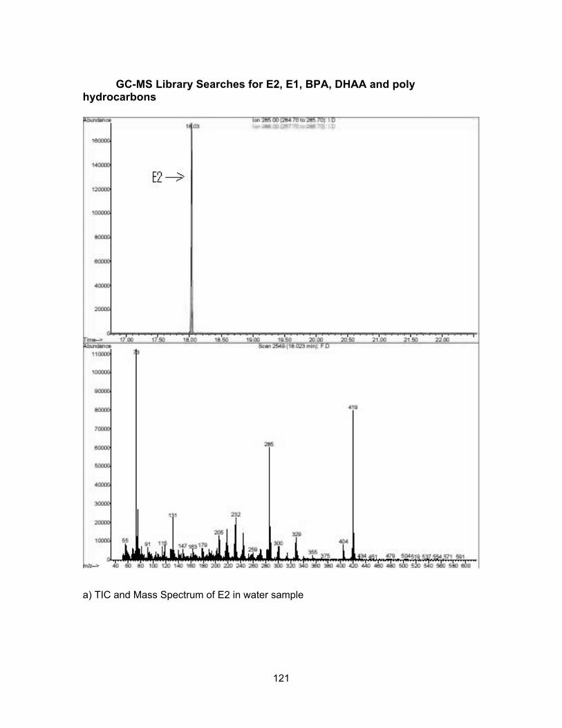
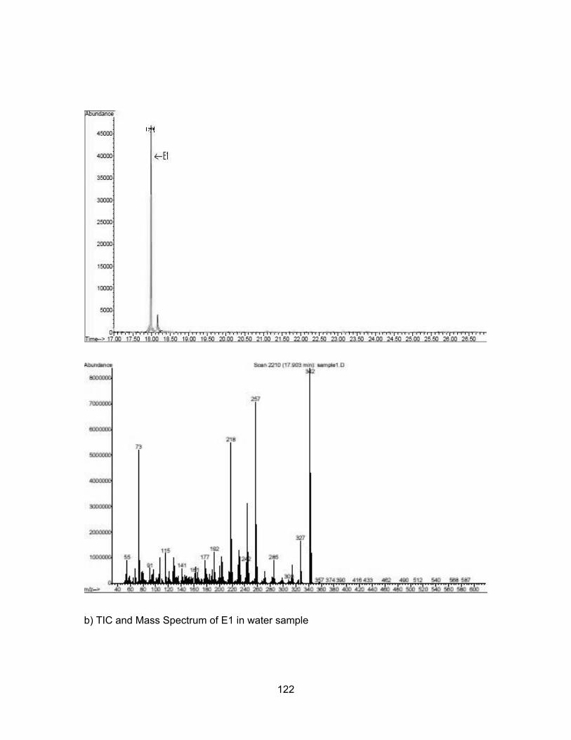
samples to identify specific compounds in the mixture. The chemicals identified were 17β-

estradiol, estrone, bisphenol A and dehydroabietic acid. Findings from this study may be

used as benchmark levels for future studies in the same region.

Keywords: EDCs, Recombinant yeast bioassays, steroid hormones, AhR agonists

Acknowledgements

I thank Allah for all the help in the completion of this research. I am also grateful to my

senior supervisor Dr. Francis Law for entrusting and guiding me throughout on this

project. Your guidance and advice on my work has been invaluable. I am equally grateful

to my supervisor Dr. Margo Moore for her constructive feedback and guidance on both

my research and thesis. My sincere thanks goes to Dr. Chris Kennedy for always

providing me with productive feedback in labs and classrooms. I also want to thank Dr.

Felix Breden for giving me opportunities to learn and explore science. My special

gratitude goes to Dr. Zaheer Khan for providing support and encouragements on my

work.

I want to acknowledge the generosity of my colleagues Zeyad Alehaideb, Noor Fageh

and Alvin Louie. Many thanks go to Marlene Nguyen for her support during my grad

years and Debbie Sandher for her guidance in my undergraduate years. I am forever

thankful to Tammy McMullan and Thelma Finlayson for their advice and assistance

during my time at the university.

Last but not least, I want to thank Kristina Pohl, Kristen Fay Gorman and Ben Sandkam

for giving me a great company and memories that will be cherished forever.

iv

v

Table of Contents

Approval .............................................................................................................................ii Abstract ............................................................................................................................. iii Acknowledgements ...........................................................................................................iv Table of Contents .............................................................................................................. v List of Tables .................................................................................................................... vii List of Figures.................................................................................................................. viii List of Acronyms ................................................................................................................ x

1. Introduction .............................................................................................................. 1 1.1 The Endocrine System and Endocrine Disrupting Compounds ............................... 1 1.2 Four classes of EDCs in the environment ................................................................ 2

1.2.1 Estrogenic Compounds ................................................................................ 2 1.2.2 Androgenic Compounds ............................................................................... 5 1.2.3 Glucocorticoid Compounds .......................................................................... 7 1.2.4 Aryl Hydrocarbon Receptor (AhR) Agonists ................................................. 9

1.3 Yeast Screening Bioassays.................................................................................... 10 1.4 Research Objectives and Study areas ................................................................... 11

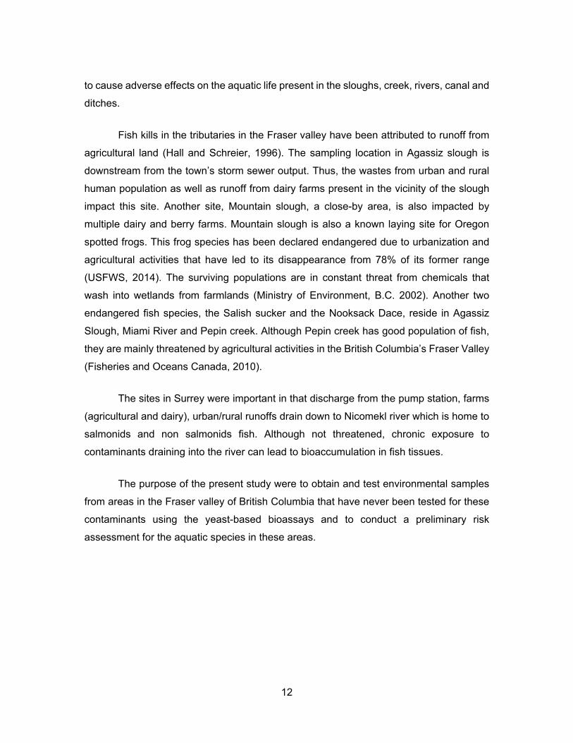
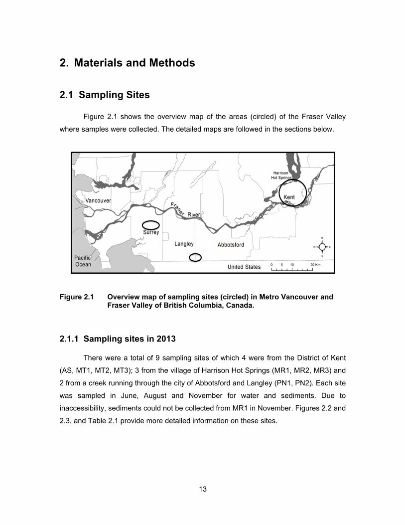
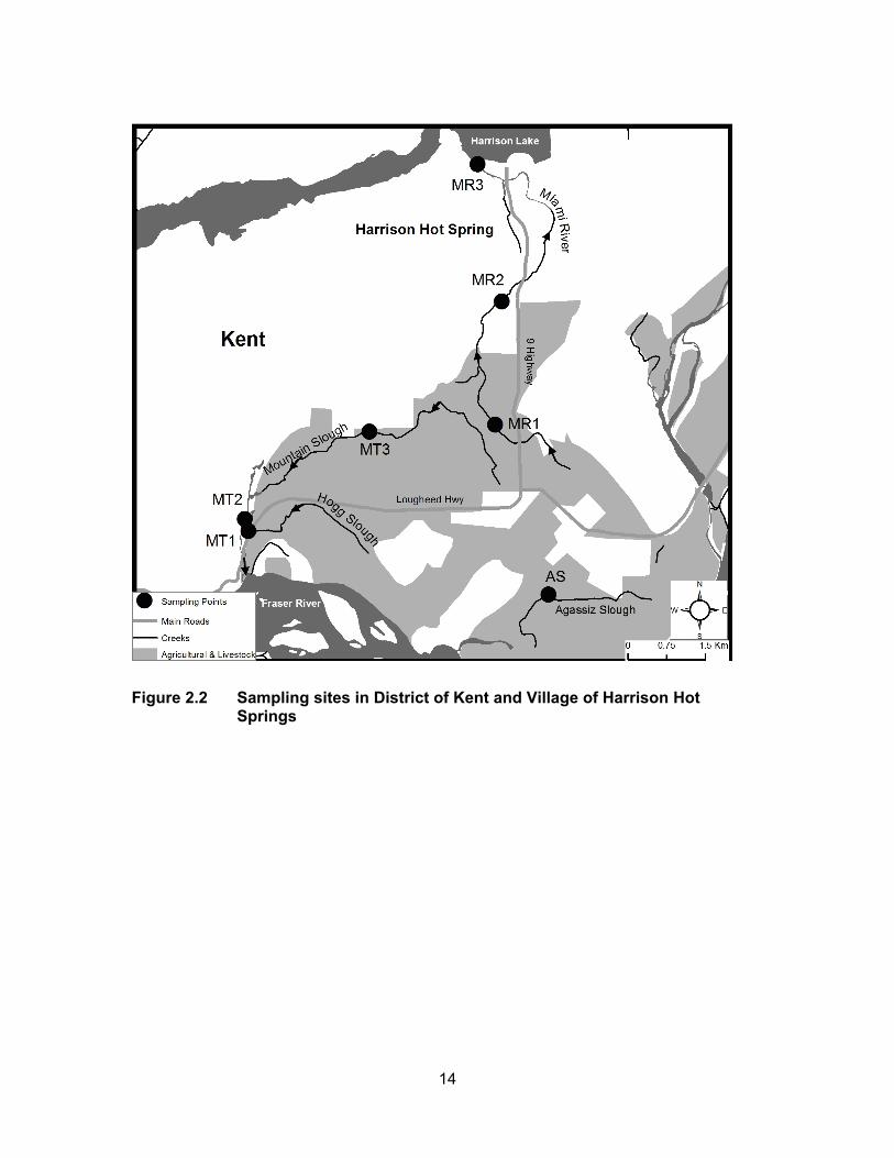
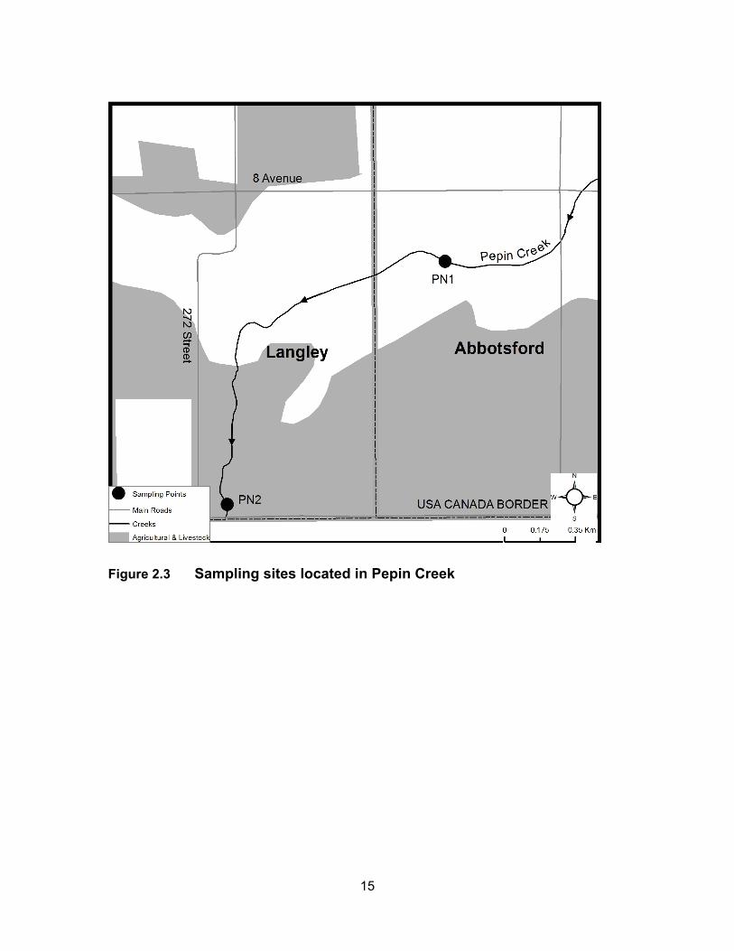
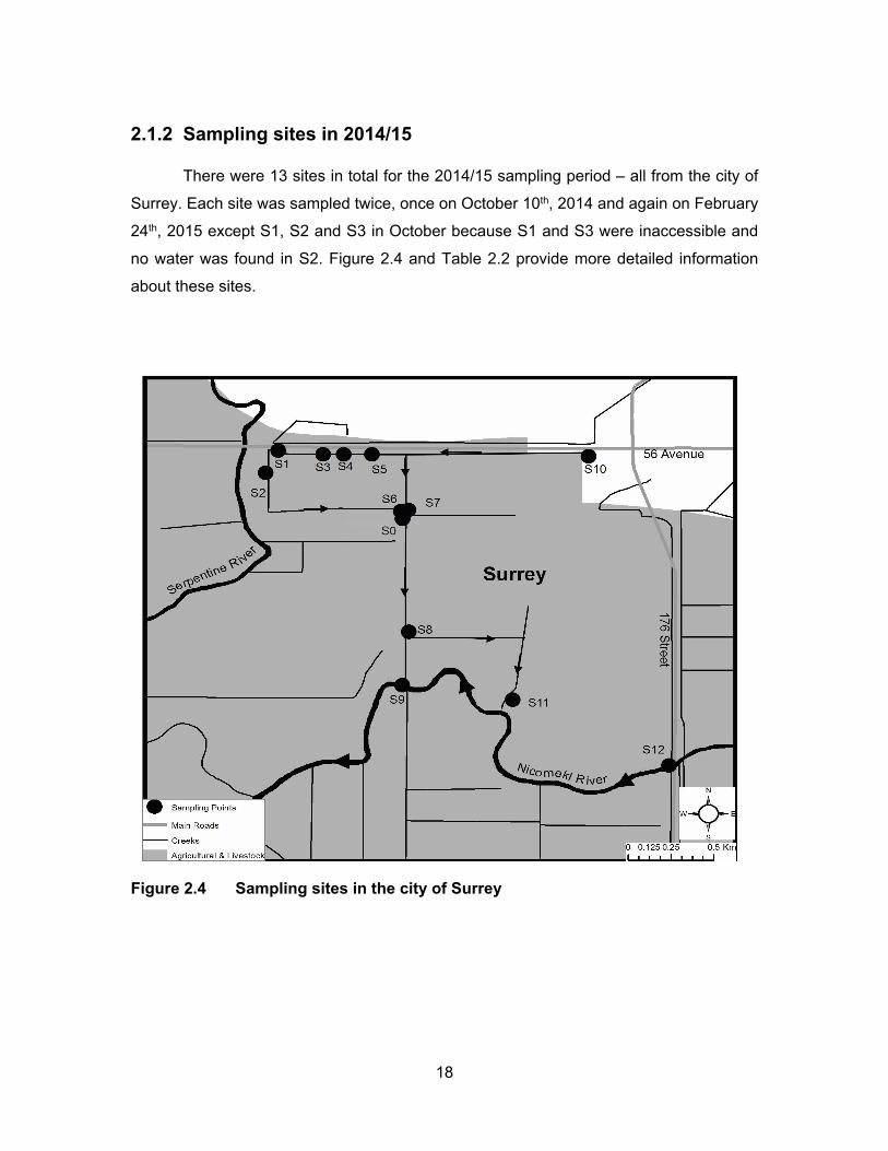
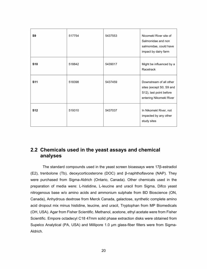
2. Materials and Methods .......................................................................................... 13 2.1 Sampling Sites ....................................................................................................... 13

2.1.1 Sampling sites in 2013 ............................................................................... 13 2.1.2 Sampling sites in 2014/15 .......................................................................... 18

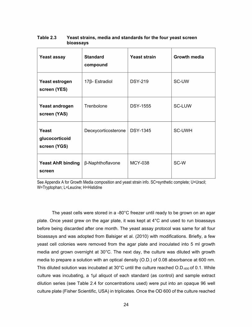
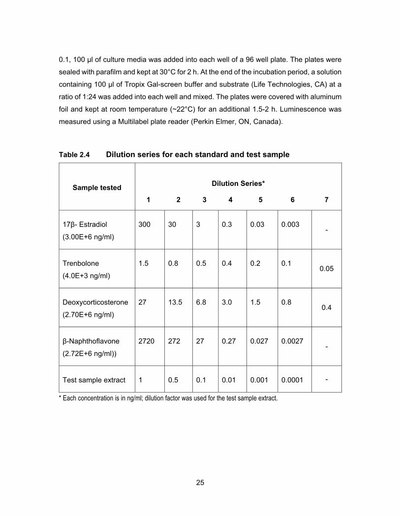
2.2 Chemicals used in the yeast assays and chemical analyses ................................. 20 2.3 Sample storage and extraction ............................................................................... 21 2.4 Protocol for the yeast screen bioassays ................................................................. 22 2.5 Calculation and data analysis ................................................................................. 26 2.6 Gas chromatography-mass spectrometry analyses ............................................... 27

2.6.1 GC-MS analysis of estrogenic compounds ................................................ 27 2.6.2 GC-MS analysis of androgenic compounds ............................................... 28 2.6.3 GC-MS analysis of polyaromatic hydrocarbon compounds ....................... 28 2.6.4 GC-MSD conditions .................................................................................... 28

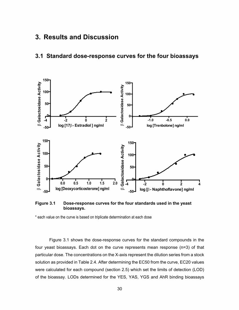
3. Results and Discussion ......................................................................................... 30 3.1 Standard dose-response curves for the four bioassays ......................................... 30 3.2 Recovery and accuracy test for the four recombinant yeast bioassays ................. 33 3.3 EDCs levels from sampling sites in 2013 ............................................................... 35

3.3.1 Estrogenic levels in water and sediments .................................................. 35 3.3.1.1 Estrogenic levels in water ....................................................................... 35 3.3.1.2 Estrogenic levels in sediments ............................................................... 37

3.3.2 Androgenic levels in water and sediments ................................................. 42 3.3.2.1 Androgenic levels in water ...................................................................... 42 3.3.2.2 Androgenic levels in sediments .............................................................. 43

3.3.3 Glucocorticoid levels in water and sediments ............................................ 48 3.3.3.1 Glucocorticoid levels in water ................................................................. 48 3.3.3.2 Glucocorticoid levels in sediments ......................................................... 49

vi

3.3.4 Aryl hydrocarbon receptor agonists levels in water and sediments ........... 54 3.3.4.1 AhR agonists levels in water .................................................................. 54 3.3.4.2 AhR agonists levels in sediments ........................................................... 55

3.4 EDCs levels from sampling sites in 2014/15 .......................................................... 61 3.4.1 Estrogenic levels in water and sediments .................................................. 61

3.4.1.1 Estrogenic levels in water ....................................................................... 61 3.4.1.2 Estrogenic levels in sediments ............................................................... 62

3.4.2 Androgenic levels in water and sediments ................................................. 65 3.4.2.1 Androgenic levels in water ...................................................................... 66 3.4.2.2 Androgenic levels in sediments .............................................................. 66

3.4.3 Glucocorticoid levels in water and sediments ............................................ 69 3.4.3.1 Glucocorticoid levels in water ................................................................. 69 3.4.3.2 Glucocorticoid levels in sediments ......................................................... 70

3.4.4 Aryl Hydrocarbon receptor agonists levels in water and sediments ........... 74 3.4.4.1 AhR agonists levels in water .................................................................. 75 3.4.4.2 AhR agonists levels in sediments ........................................................... 75

3.5 Results from Chemical Analyses ............................................................................ 78

4. Risk to exposed species ....................................................................................... 84

5. Study Limitations and Future Directions ............................................................. 86

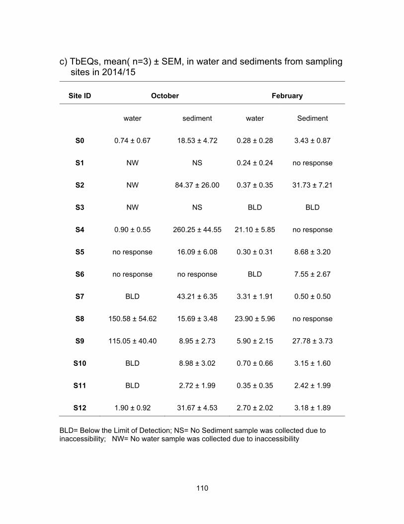
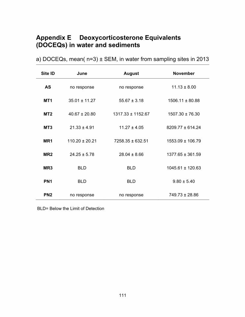
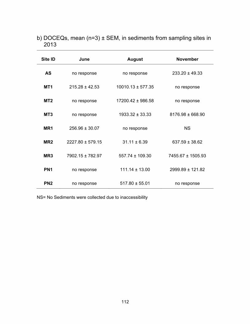
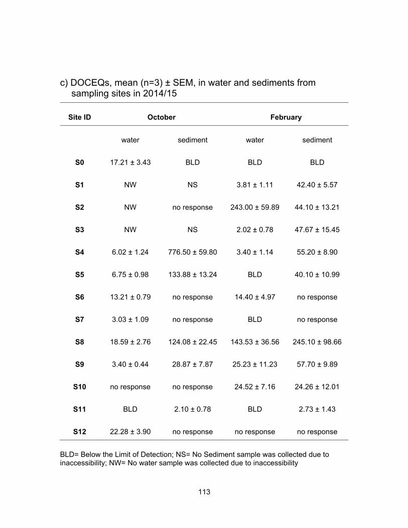
References .................................................................................................................. 87 Appendix A Yeast strains and Media preparations ...................................................... 99 Appendix B Rainfall data ............................................................................................ 101 Appendix C Estradiol Equivalents (EEQs) in water and sediments ........................... 105 Appendix D Trenbolone Equivalents (TbEQs) in water and sediments ..................... 108 Appendix E Deoxycorticosterone Equivalents (DOCEQs) in water and

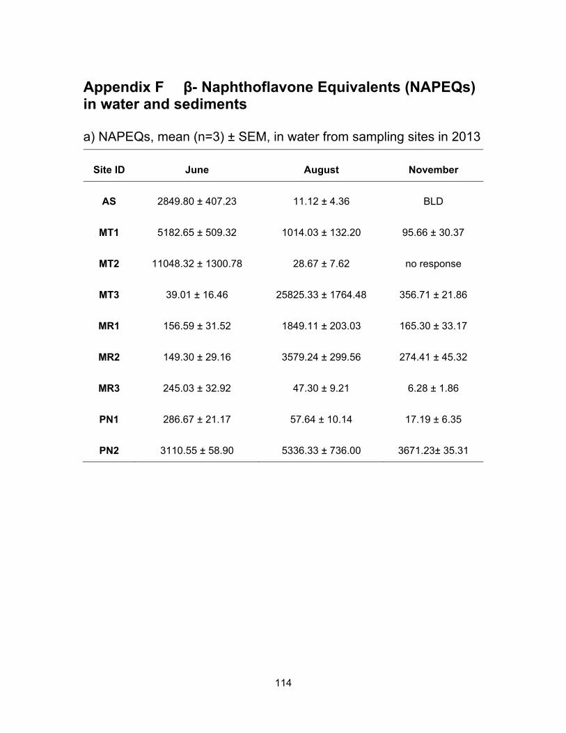
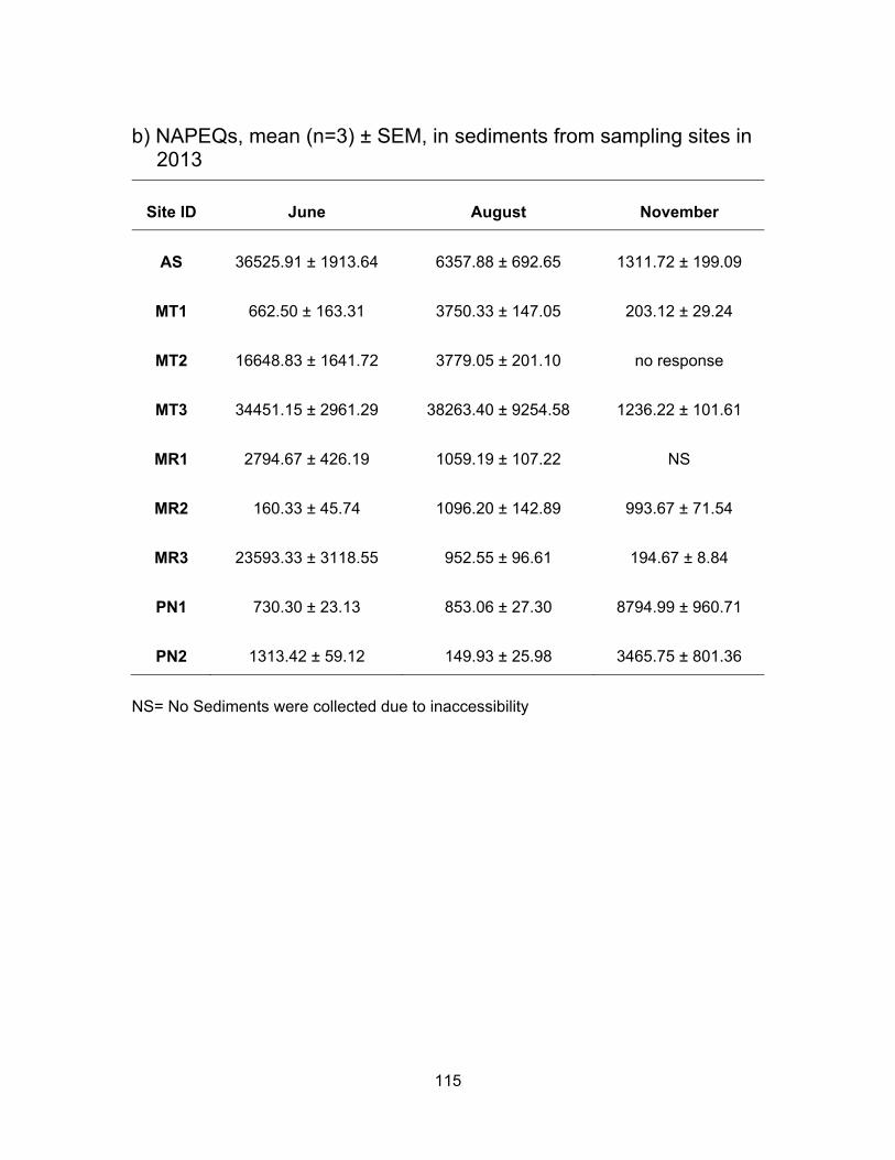
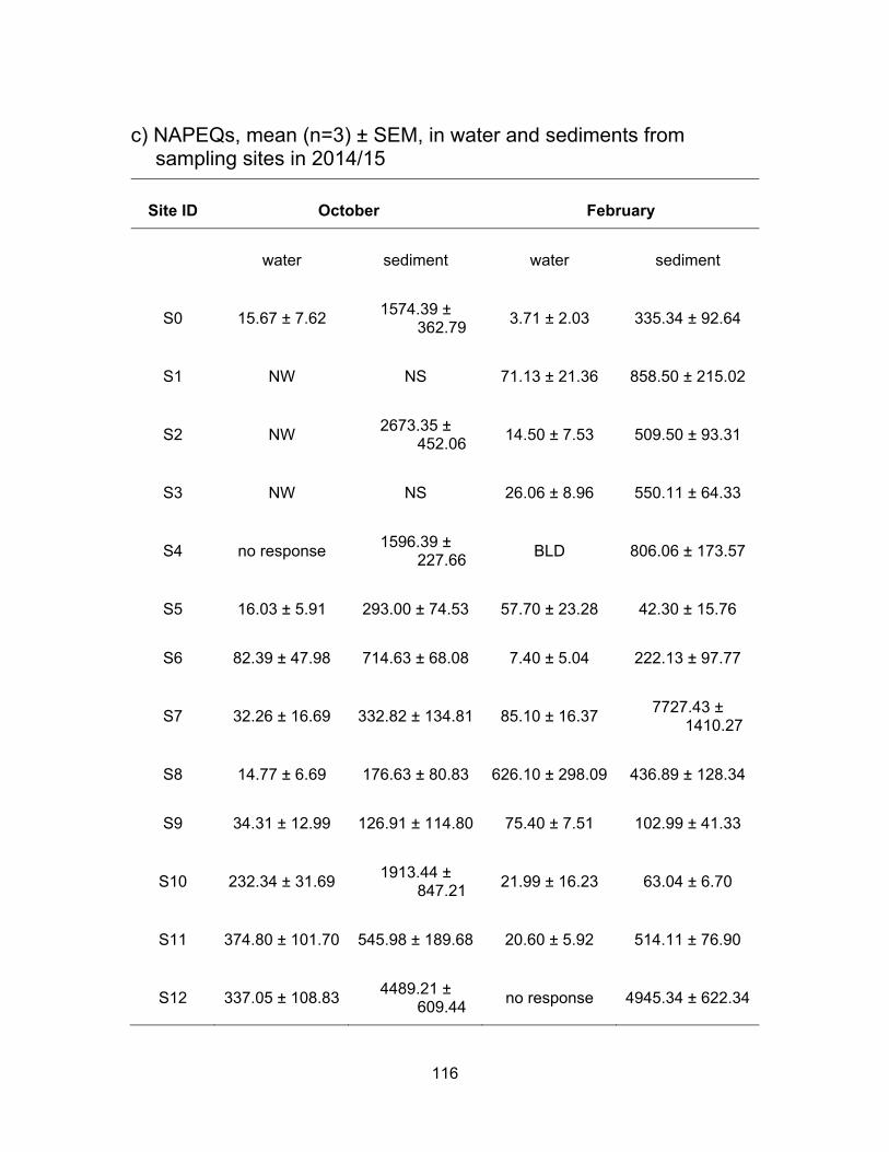
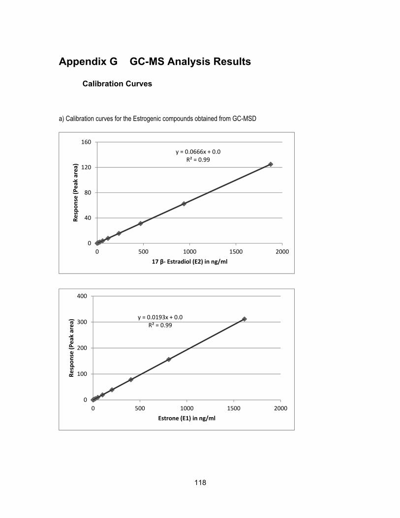
sediments ............................................................................................................. 111 Appendix F β- Naphthoflavone Equivalents (NAPEQs) in water and sediments ....... 114 Appendix G GC-MS Analysis Results ........................................................................ 118

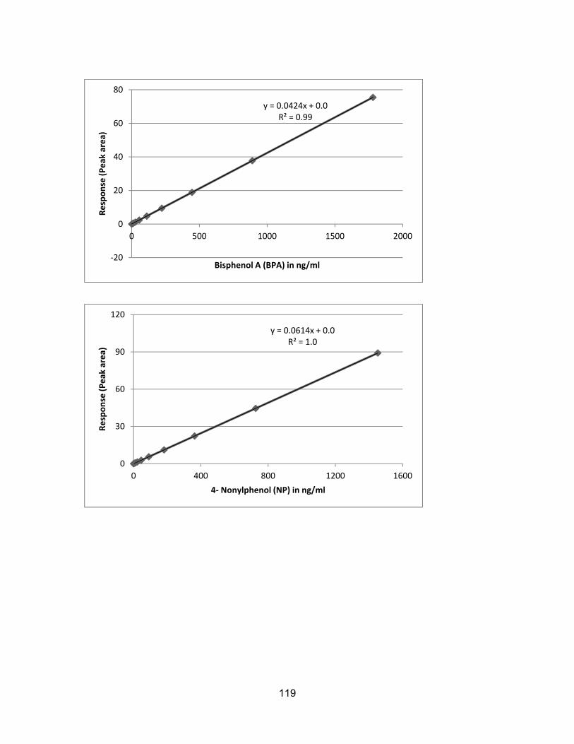
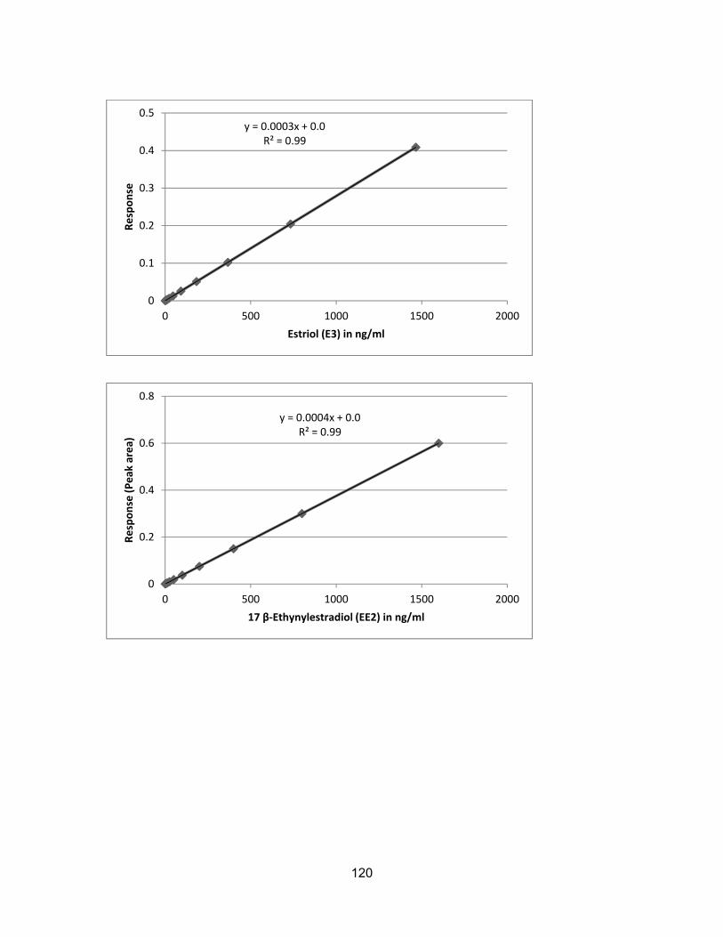
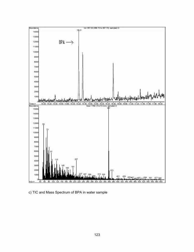
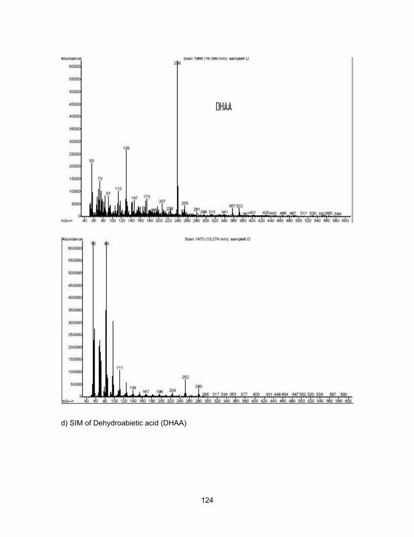
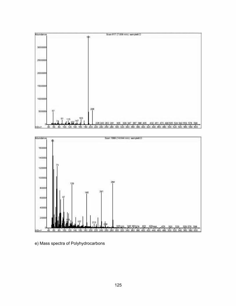
Calibration Curves ................................................................................................ 118 GC-MS Library Searches for E2, E1, BPA, DHAA and poly hydrocarbons .......... 121

vii

List of Tables

Table 1.1 Example of natural and synthetic estrogenic compounds ......................... 5

Table 1.2 Example of natural and synthetic androgenic compounds ........................ 7

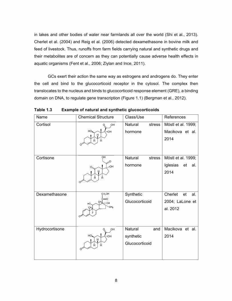
Table 1.3 Example of natural and synthetic glucocorticoids ...................................... 8

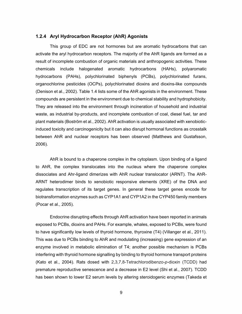
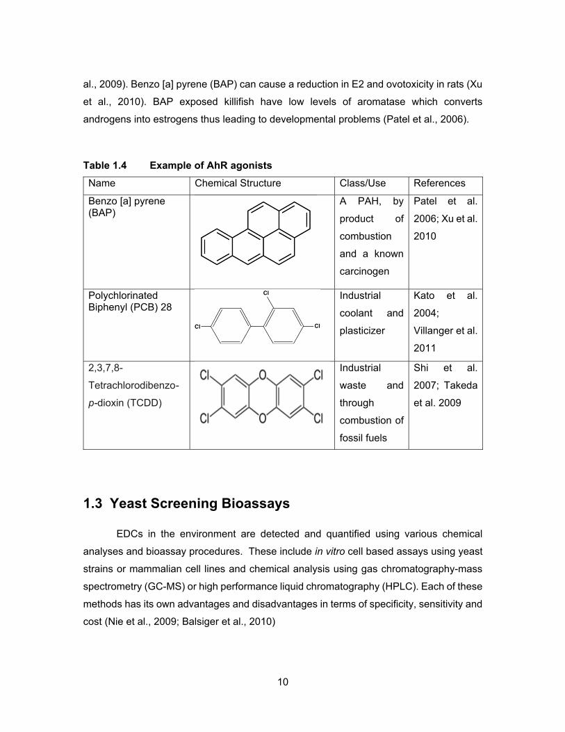
Table 1.4 Example of AhR agonists ........................................................................ 10

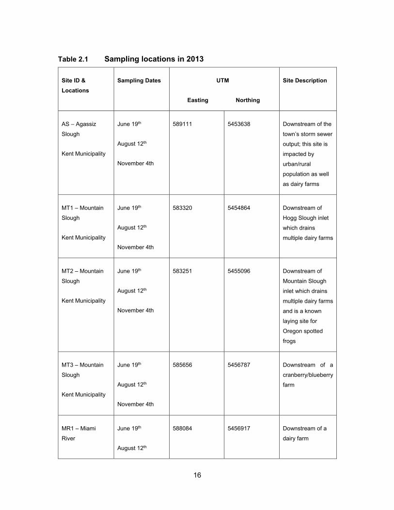
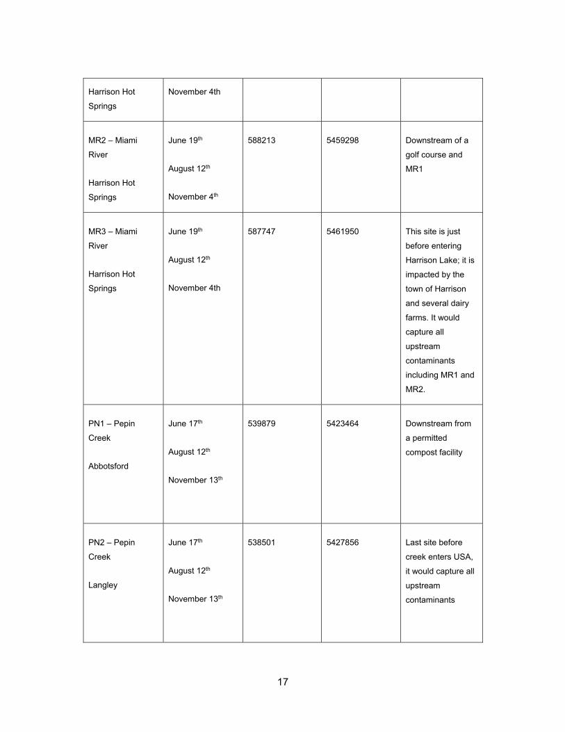
Table 2.1 Sampling locations in 2013 ...................................................................... 16

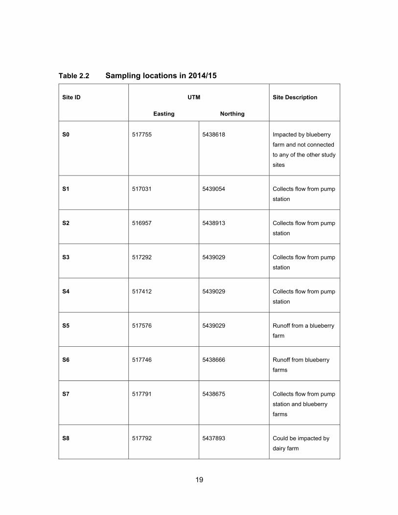
Table 2.2 Sampling locations in 2014/15 ................................................................. 19

Table 2.3 Yeast strains, media and standards for the four yeast screen bioassays ............................................................................................ 24

Table 2.4 Dilution series for each standard and test sample ................................... 25

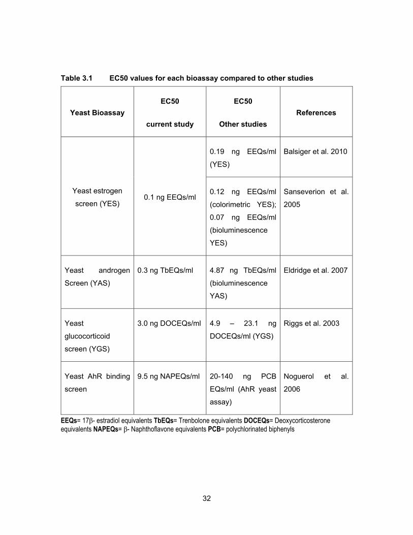
Table 3.1 EC50 values for each bioassay compared to other studies .................... 32

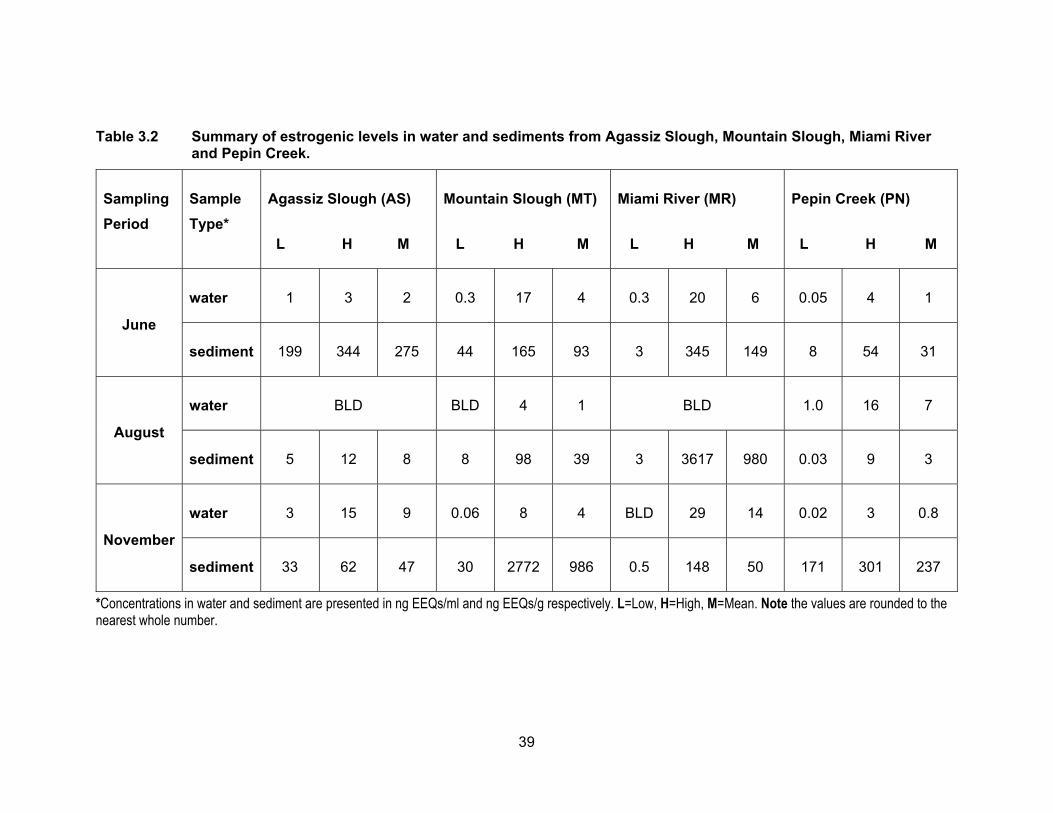
Table 3.2 Summary of estrogenic levels in water and sediments from Agassiz Slough, Mountain Slough, Miami River and Pepin Creek. ................................................................................................. 39

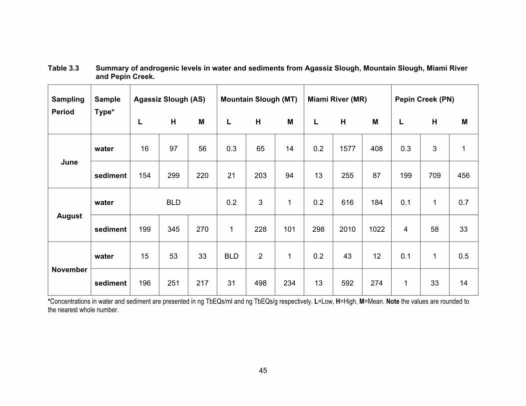
Table 3.3 Summary of androgenic levels in water and sediments from Agassiz Slough, Mountain Slough, Miami River and Pepin Creek. ................................................................................................. 45

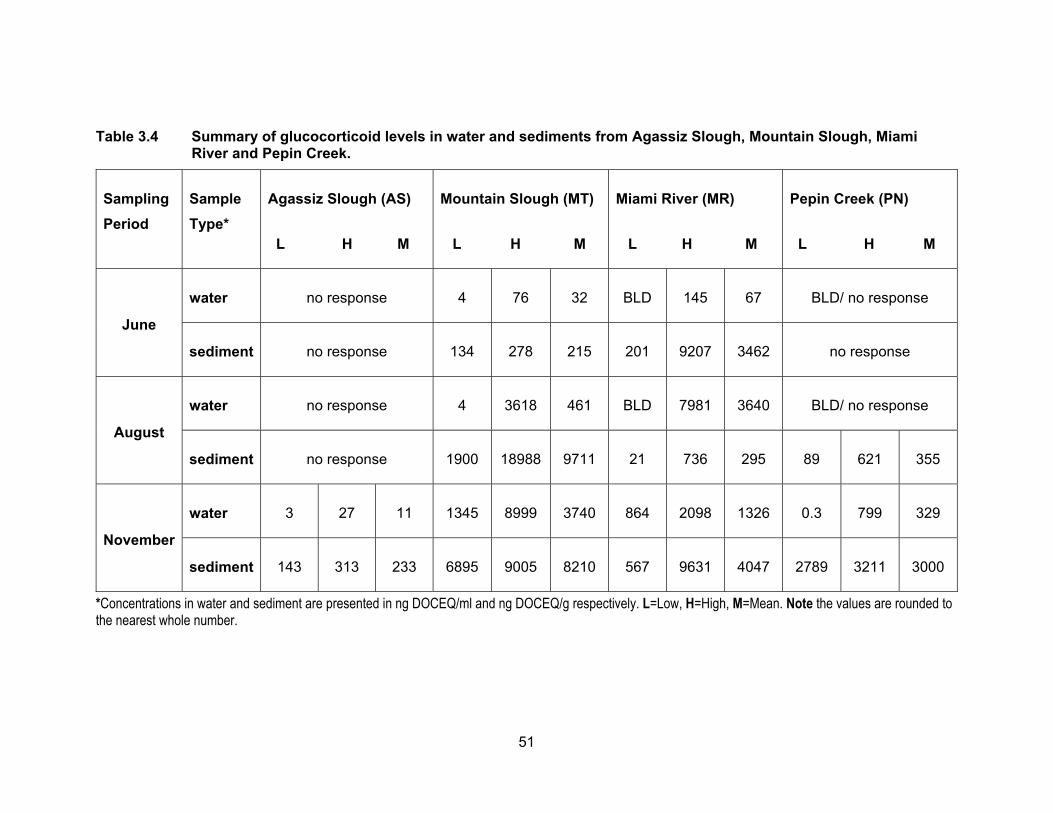
Table 3.4 Summary of glucocorticoid levels in water and sediments from Agassiz Slough, Mountain Slough, Miami River and Pepin Creek. ................................................................................................. 51

Table 3.5 Summary of AhR agonists levels in water and sediments from Agassiz Slough, Mountain Slough, Miami River and Pepin Creek. ................................................................................................. 58

Table 3.6 Summary of mean estrogenic levels from sites in Surrey. ...................... 63

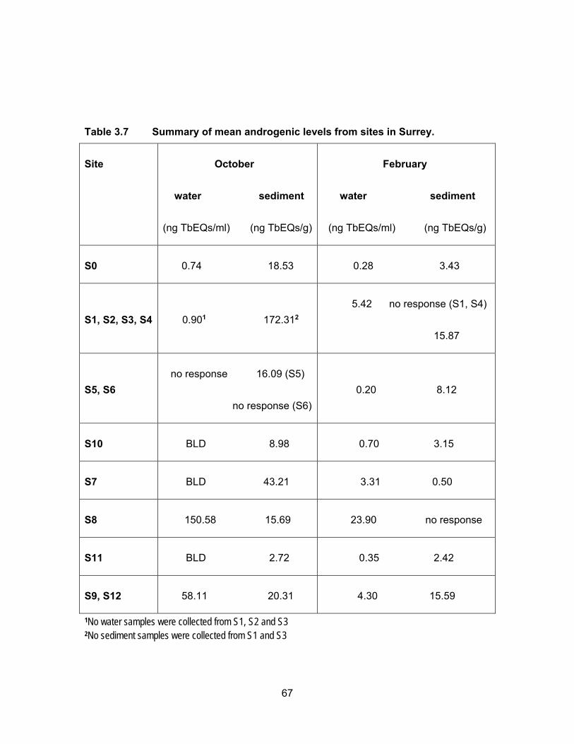
Table 3.7 Summary of mean androgenic levels from sites in Surrey. ..................... 67

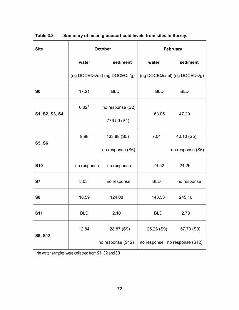
Table 3.8 Summary of mean glucocorticoid levels from sites in Surrey. ................. 72

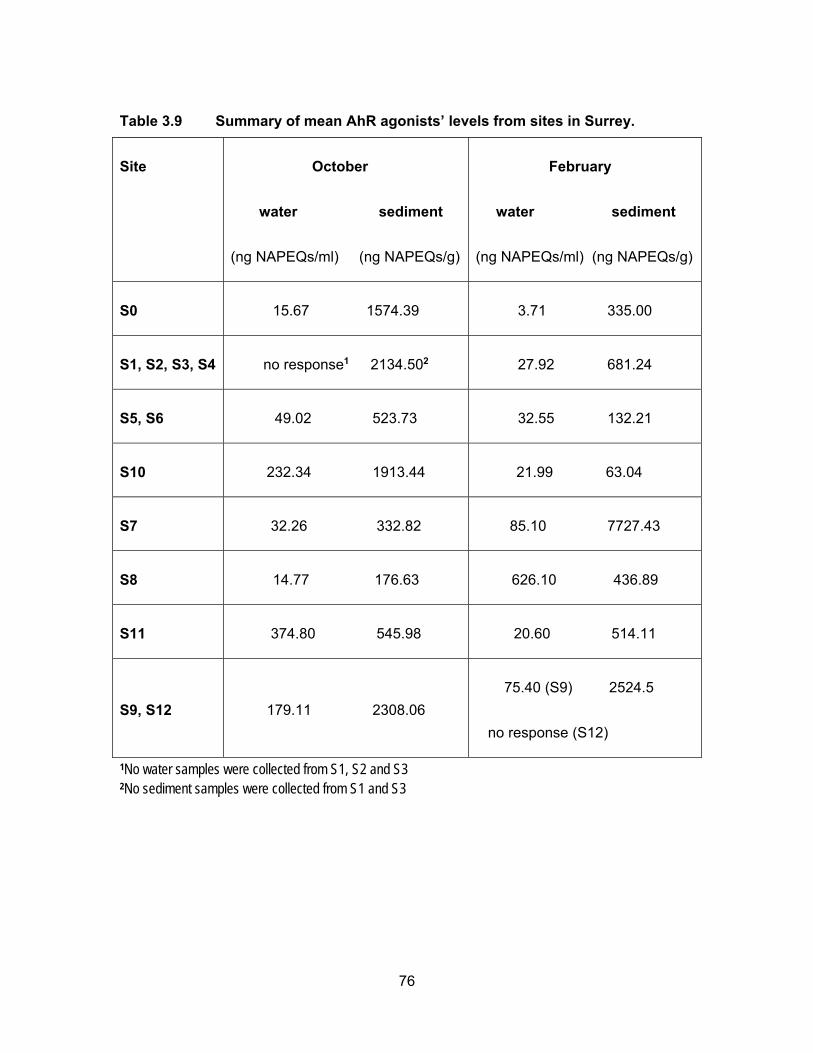
Table 3.9 Summary of mean AhR agonists’ levels from sites in Surrey. ................. 76

viii

List of Figures

Figure 1.1 Schematic diagram of steroid hormones’ mode of action. ....................... 3

Figure 2.1 Overview map of sampling sites (circled) in Metro Vancouver and Fraser Valley of British Columbia, Canada. ........................................ 13

Figure 2.2 Sampling sites in District of Kent and Village of Harrison Hot Springs ................................................................................................ 14

Figure 2.3 Sampling sites located in Pepin Creek ................................................... 15

Figure 2.4 Sampling sites in the city of Surrey ........................................................ 18

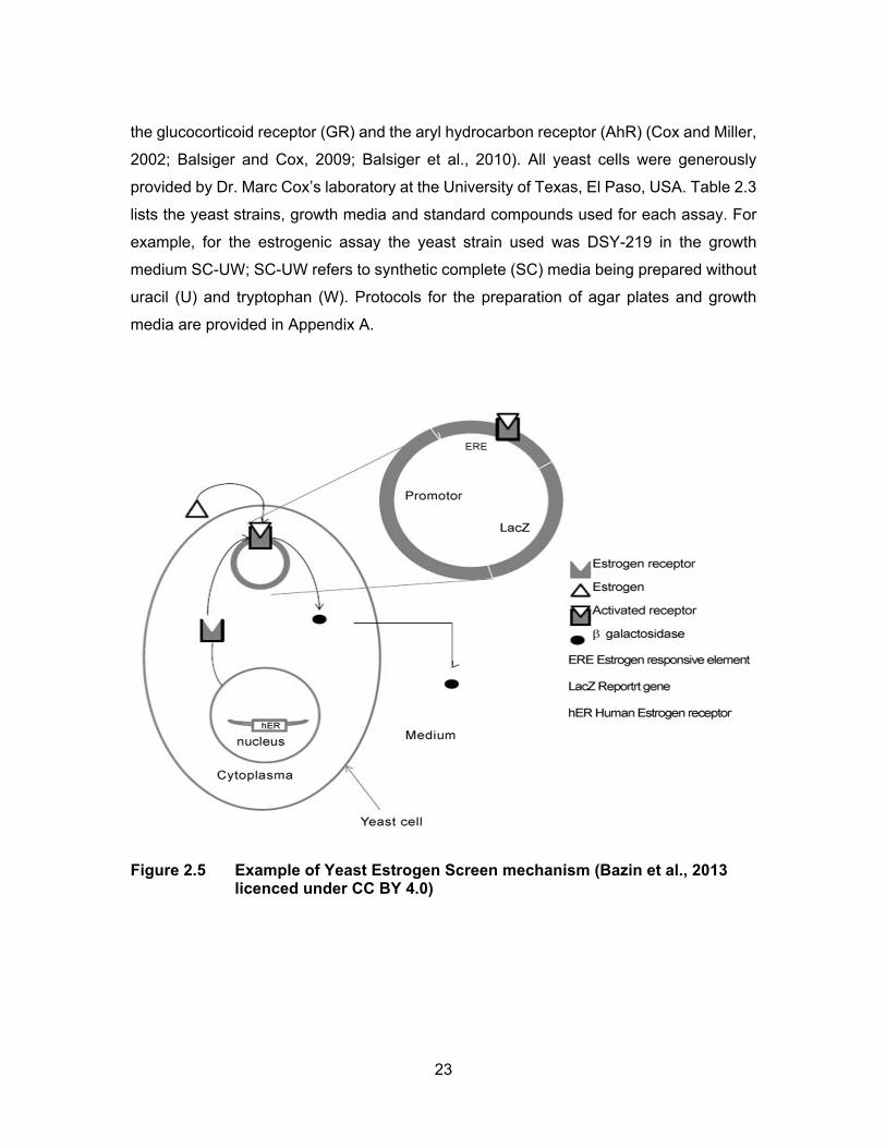
Figure 2.5 Example of Yeast Estrogen Screen mechanism (Bazin et al., 2013 licenced under CC BY 4.0) ........................................................ 23

Figure 3.1 Dose-response curves for the four standards used in the yeast bioassays. ........................................................................................... 30

Figure 3.2 Concentrations recovered (± SEM) for each bioassay. .......................... 34

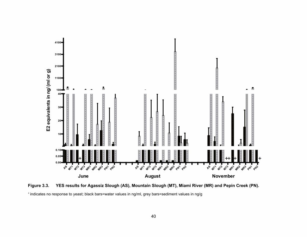
Figure 3.3. YES results for Agassiz Slough (AS), Mountain Slough (MT), Miami River (MR) and Pepin Creek (PN). ........................................... 40

Figure 3.4. Sites in 2013 sampling period with EEQs levels shown as dots. .......... 41

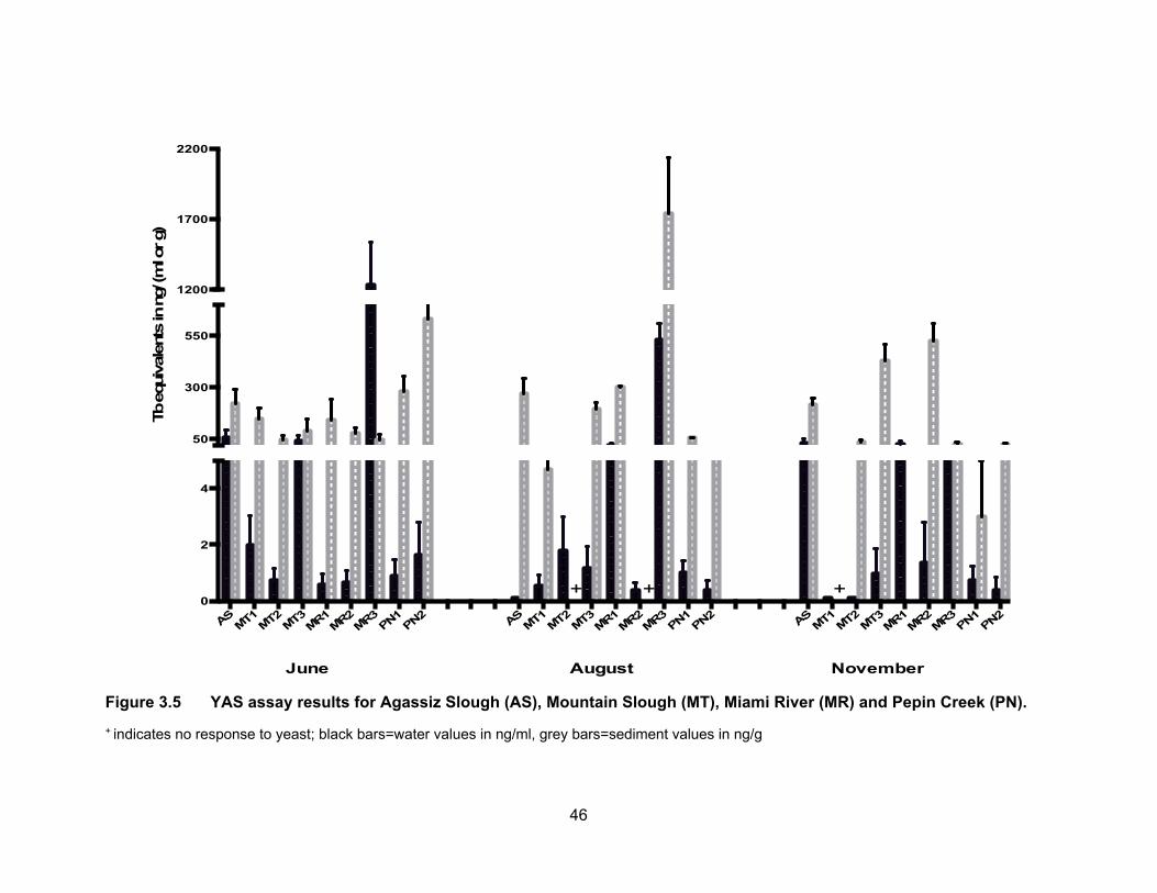
Figure 3.5 YAS assay results for Agassiz Slough (AS), Mountain Slough (MT), Miami River (MR) and Pepin Creek (PN). ................................. 46

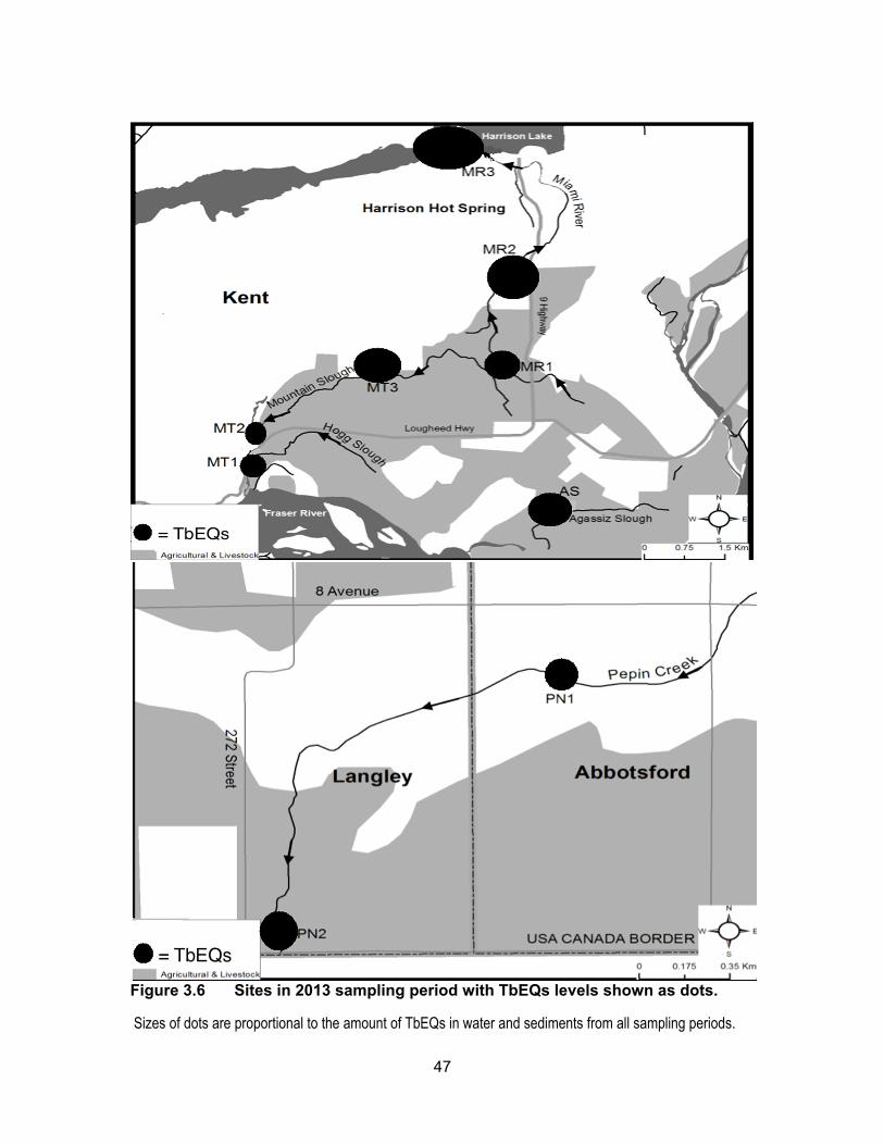
Figure 3.6 Sites in 2013 sampling period with TbEQs levels shown as dots. ......... 47

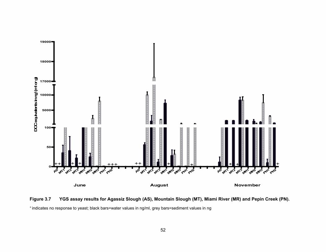
Figure 3.7 YGS assay results for Agassiz Slough (AS), Mountain Slough (MT), Miami River (MR) and Pepin Creek (PN). ................................. 52

Figure 3.8 Sites in 2013 sampling period with DOCEQs levels shown as dots. ................................................................................................... 53

Figure 3.9 AhR assay results for Agassiz Slough (AS), Mountain Slough (MT), Miami River (MR) and Pepin Creek (PN). ................................. 59

Figure 3.10 Sites in 2013 sampling period with NAPEQs levels shown as dots. ................................................................................................... 60

Figure 3.11 YES assay results for sites in Surrey. .................................................. 64

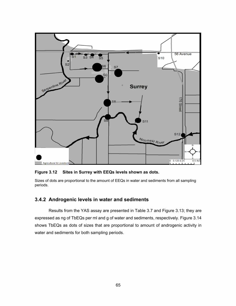
Figure 3.12 Sites in Surrey with EEQs levels shown as dots. ................................. 65

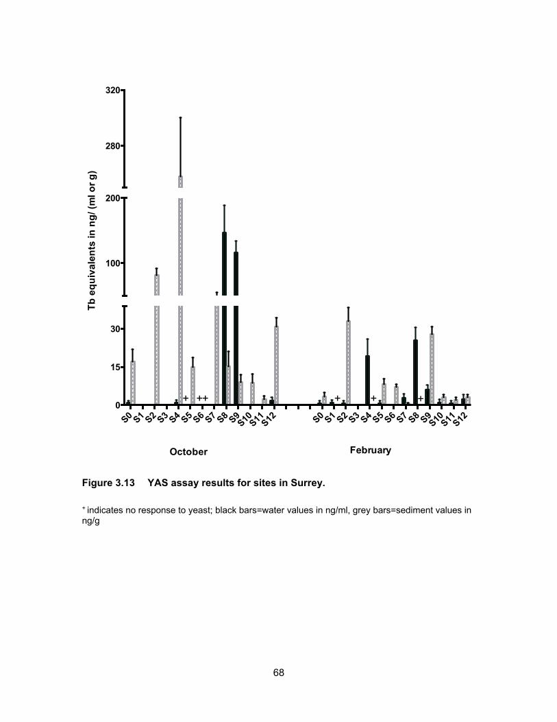
Figure 3.13 YAS assay results for sites in Surrey. .................................................. 68

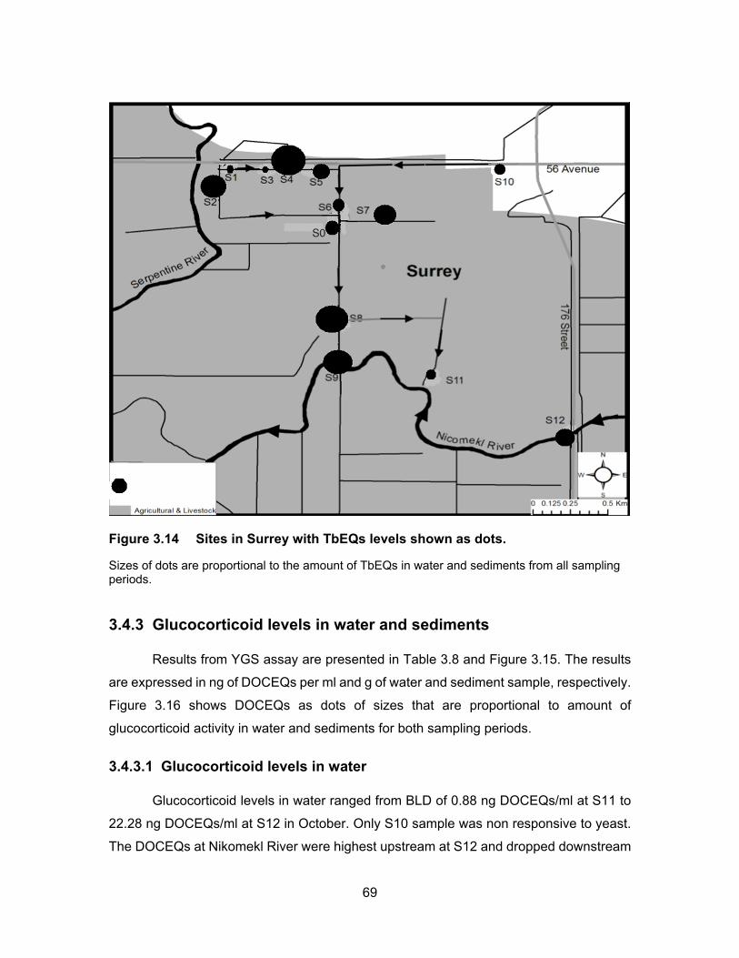
Figure 3.14 Sites in Surrey with TbEQs levels shown as dots. ............................... 69

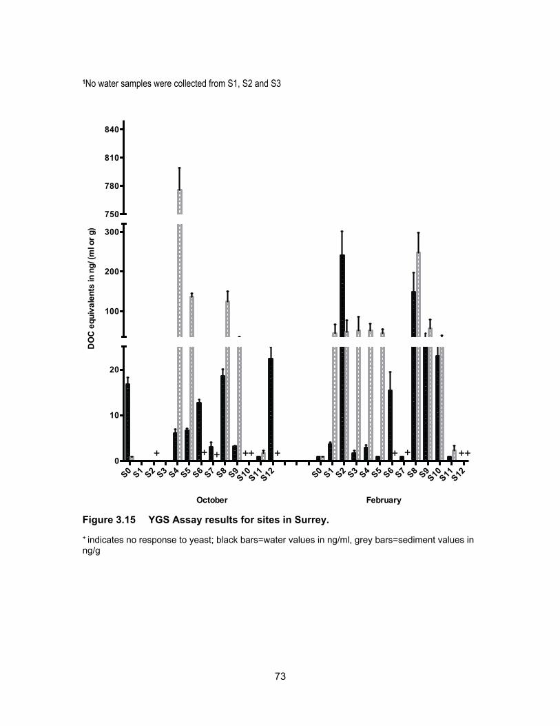
Figure 3.15 YGS Assay results for sites in Surrey. ................................................. 73

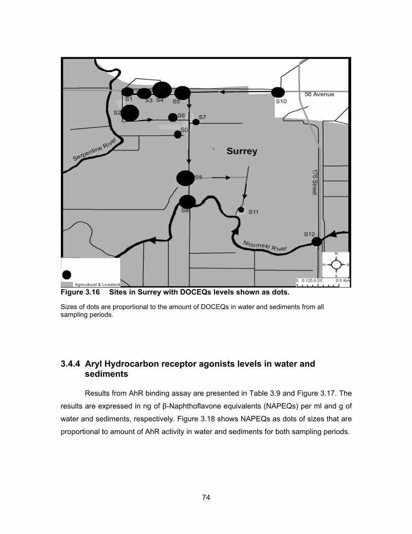
Figure 3.16 Sites in Surrey with DOCEQs levels shown as dots. ........................... 74

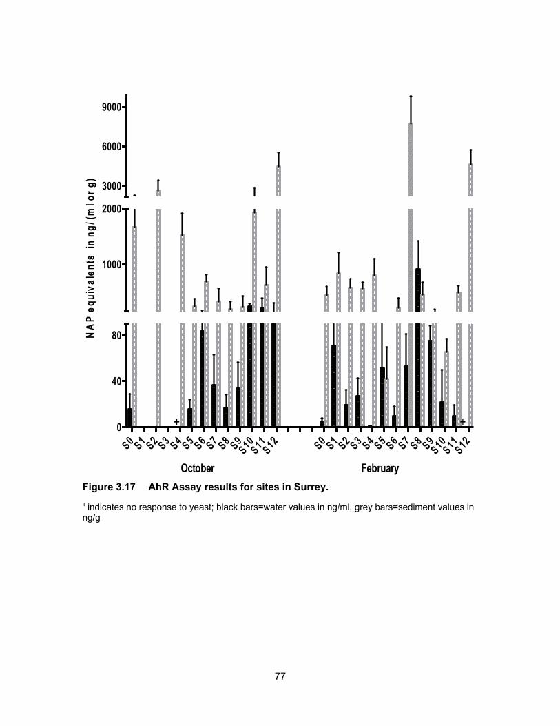
Figure 3.17 AhR Assay results for sites in Surrey. .................................................. 77

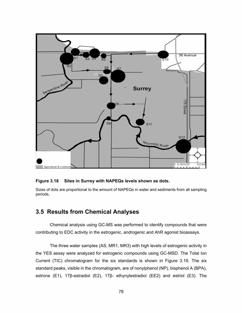
Figure 3.18 Sites in Surrey with NAPEQs levels shown as dots. ............................ 78

ix

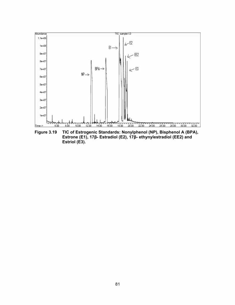
Figure 3.19 TIC of Estrogenic Standards: Nonylphenol (NP), Bisphenol A (BPA), Estrone (E1), 17β- Estradiol (E2), 17β- ethynylestradiol (EE2) and Estriol (E3). ........................................................................ 81

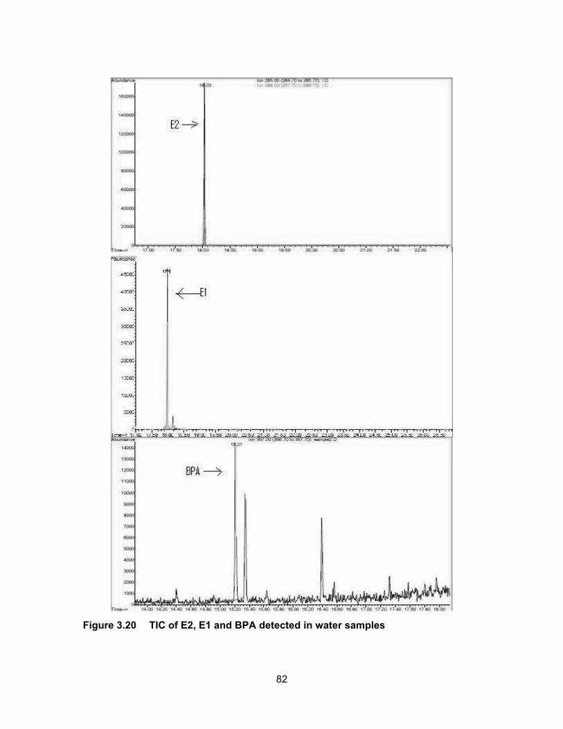
Figure 3.20 TIC of E2, E1 and BPA detected in water samples .............................. 82

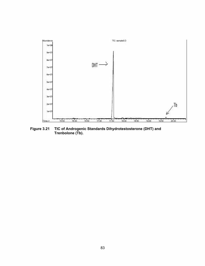
Figure 3.21 TIC of Androgenic Standards Dihydrotestosterone (DHT) and Trenbolone (Tb). ................................................................................. 83

x

List of Acronyms

AhR Aryl Hydrocarbon Receptor

ANOVA Analysis of Variance

AR Androgen Receptor

ARNT Aryl hydrocarbon Receptor Nuclear Translocator

BLD Below the Limit of Detection

CALUX Chemical Activated Luciferase gene expression

DHT Dihydrotestosterone

DHTEQ Dihydrotestosterone Equivalent

DOC Deoxycorticosterone

DOCEQ Deoxycorticosterone Equivalent

E2 17β- Estradiol

EC50 Effective Concentration at 50% of maximal activity

EDC Endocrine Disrupting Chemicals/Compounds

EEQ 17β- Estradiol Equivalent

ER Estrogen Receptor

GC/MS Gas Chromatography- Mass Spectrometry

GR Glucocorticoid Receptor

HPA Hypothalamic-Pituitary-Adrenal axis

HPGL Hypothalamus-Pituitary-Gonadal-Liver axis

HPI Hypothalamus-Pituitary-Interrenal axis

HPT Hypothalamus-Pituitary-Thyroid axis

NAP β- Naphthoflavone

NAPEQ β- Naphthoflavone Equivalent

PAH Polyaromatic Hydrocarbon

PCB Polychlorinated Biphenyl

SEM Standard Error of the Mean

WWTP Waste Water Treatment Plant

YAS Yeast Androgen Screen

YES Yeast Estrogen Screen

YGS Yeast Glucocorticoid Screen

1

1. Introduction

Over the last couple of decades, much has been written about endocrine disrupting

compounds (EDCs) and their potential deleterious effects in humans and animals. EDCs

are ubiquitous in the environment; they have been found in plastic bottles, metal food

cans, detergents, flame retardants, food additives, cosmetics, pesticides, herbicides, etc.

Therefore, many living organisms are exposed to EDCs on a daily basis. Evidence is

accumulating to indicate that EDCs such as synthetic estrogens, anabolic steroids, anti-

inflammatory drugs, polychlorinated biphenyls (PCBs), bisphenol A (BPA), nonylpheol

(NP) and some pesticides can disrupt the development and growth of terrestrial and

aquatic animals (Damstra et al., 2002; Hayes et al., 2005; Lintelmann et al., 2003). Some

of the adverse effects include demasculinization and feminization of fish, decreased

hatching success in fish and birds, abnormal thyroid function, and alteration of immune

and behavioral functions in fish, birds and mammals (Tierney et al., 2014).

Surprisingly, there have been very few studies on the presence and effects of

EDCs in lakes, sloughs, creeks and other small bodies of water (Rosen et al., 2006;

Bogdal et al., 2009). A recent experiment in a Canadian lake has shown adverse health

effects in a fish population after dosing the lakes with a very low concentration (2 ng/L) of

17 α-ethynylestradiol (EE2) (Kidd et al., 2007; Palace et al., 2009).

1.1 The Endocrine System and Endocrine Disrupting Compounds

The endocrine system (ES) is an organ system that involves similar glands,

hormones and secretion patterns in vertebrates from fish to mammals (Campbell et al.,

2004). The ES consists of an internal network of signals and responses that are crucial in

maintaining and regulating homeostasis and other bodily functions. The endocrine glands

include the hypothalamus, pituitary, pineal, thyroid, parathyroid, adrenal cortex and

medulla, pancreas, chromaffin tissue (fish), corpuscles of Stannius (fish), the interrenal

2

organ (fish) as well as male and female reproductive organs. These glands release

hormones, chemical messengers that travel in the blood to other parts of the body, to

control essential functions such as metabolism, growth, development, reproduction,

primary and secondary sexual characteristics, as well as water, calcium, and glucose

balance.

U.S. Environmental Protection Agency (USEPA) defines EDC as “an exogenous

agent that interferes with synthesis, secretion, transport, metabolism, binding action, or

elimination of natural blood-borne hormones that are present in the body and are

responsible for homeostasis, reproduction, and developmental process.” Thus EDCs act

in several ways to interfere with the internal hormonal system. They can mimic hormones

and disrupt the normal functioning of an ES. They can cause an over stimulation of certain

responses, or initiate a response at an inappropriate time. They can also bind to receptors

and block endogenous hormones from binding thus normal signals fail to occur. They may

act to alter the metabolism of endogenous hormones and modify the availability of

hormone receptors. EDCs can also interfere with the binding proteins that carry/transport

the endogenous hormones (Bergman et al., 2012). Overall, EDCs may impact the three

axes (i.e. Hypothalamic-Pituitary-Gonadal (HPG) axis (HPG-Liver axis in fish),

Hypothalamic-Pituitary-Adrenal (HPA) axis (HP-Interrenal axis in fish), and Hypothalamic-

Pituitary-Thyroid (HPT) axis) that balance the sex, stress and thyroid hormones leading to

immune function abnormalities (Norris and Lopez, 2011).

1.2 Four classes of EDCs in the environment

In the present study, we examined three groups of natural and synthetic steroid

hormones that enter the environment through human/animal excreta, via agricultural

waste and Waste Water Treatment Plants (WWTPs). In addition, we studied AhR agonists

from industrial wastes and anthropogenic activities.

1.2.1 Estrogenic Compounds

Estrogens are lipid-soluble chemicals that bind to the ER in the cytoplasm after

entering the cell. The ligand-receptor complex then enters the nucleus and interacts with

3

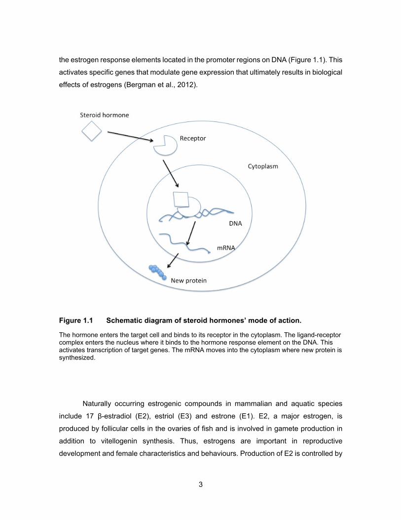
the estrogen response elements located in the promoter regions on DNA (Figure 1.1). This

activates specific genes that modulate gene expression that ultimately results in biological

effects of estrogens (Bergman et al., 2012).

Figure 1.1 Schematic diagram of steroid hormones’ mode of action.

The hormone enters the target cell and binds to its receptor in the cytoplasm. The ligand-receptor complex enters the nucleus where it binds to the hormone response element on the DNA. This activates transcription of target genes. The mRNA moves into the cytoplasm where new protein is synthesized.

Naturally occurring estrogenic compounds in mammalian and aquatic species

include 17 β-estradiol (E2), estriol (E3) and estrone (E1). E2, a major estrogen, is

produced by follicular cells in the ovaries of fish and is involved in gamete production in

addition to vitellogenin synthesis. Thus, estrogens are important in reproductive

development and female characteristics and behaviours. Production of E2 is controlled by

4

the hypothalamic-pituitary-gonadal (HPG) axis via a negative feedback mechanism that

can be modified by xenoestrogens (Hiller-Sturmhöfel and Bartke, 1998).

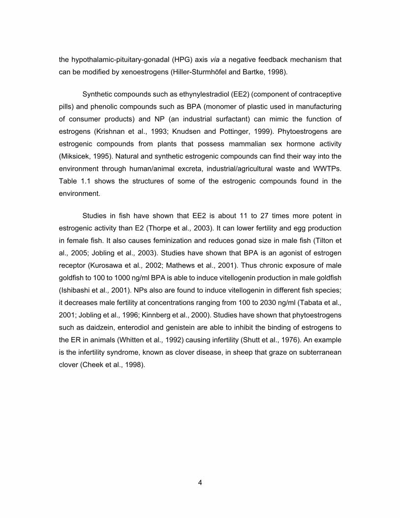
Synthetic compounds such as ethynylestradiol (EE2) (component of contraceptive

pills) and phenolic compounds such as BPA (monomer of plastic used in manufacturing

of consumer products) and NP (an industrial surfactant) can mimic the function of

estrogens (Krishnan et al., 1993; Knudsen and Pottinger, 1999). Phytoestrogens are

estrogenic compounds from plants that possess mammalian sex hormone activity

(Miksicek, 1995). Natural and synthetic estrogenic compounds can find their way into the

environment through human/animal excreta, industrial/agricultural waste and WWTPs.

Table 1.1 shows the structures of some of the estrogenic compounds found in the

environment.

Studies in fish have shown that EE2 is about 11 to 27 times more potent in

estrogenic activity than E2 (Thorpe et al., 2003). It can lower fertility and egg production

in female fish. It also causes feminization and reduces gonad size in male fish (Tilton et

al., 2005; Jobling et al., 2003). Studies have shown that BPA is an agonist of estrogen

receptor (Kurosawa et al., 2002; Mathews et al., 2001). Thus chronic exposure of male

goldfish to 100 to 1000 ng/ml BPA is able to induce vitellogenin production in male goldfish

(Ishibashi et al., 2001). NPs also are found to induce vitellogenin in different fish species;

it decreases male fertility at concentrations ranging from 100 to 2030 ng/ml (Tabata et al.,

2001; Jobling et al., 1996; Kinnberg et al., 2000). Studies have shown that phytoestrogens

such as daidzein, enterodiol and genistein are able to inhibit the binding of estrogens to

the ER in animals (Whitten et al., 1992) causing infertility (Shutt et al., 1976). An example

is the infertility syndrome, known as clover disease, in sheep that graze on subterranean

clover (Cheek et al., 1998).

5

Table 1.1 Example of natural and synthetic estrogenic compounds

Chemical

Name

Chemical Structure Class/Use References

17 β-estradiol (E2)

Natural female

hormone

Kinnberg et al.

2000; Tabata

et al. 2001

17 α-ethinyl

estradiol (EE2)

Synthetic

hormone used

as oral

contraceptive

Jobling et al.

2003; Tilton et

al. 2005; Kidd

et al. 2007

Bisphenol A

(BPA)

Plasticmonomer

in production of

certain plastic

products

Ishibashi et al.

2001; Jobling

et al. 2003

Nonylphenol

(NP)

Surfactant used

in detergents,

paints,

pesticides,

cosmetics etc.

Kinnberg et al.

2000; Tabata

et al. 2001

1.2.2 Androgenic Compounds

Like estrogens, androgens are also lipid-soluble molecules that pass through cell

membranes and bind to a specific receptor, the androgen receptor, in the cytoplasm. The

ligand-receptor complex enters the nucleus of cells and attaches to the androgen

6

response element segment of DNA (Figure 1.1). This guides the cell to produce proteins

associated with androgens (Bergman et al., 2012).

Androgenic compounds are a group of steroid hormones that stimulate the

development of male sex characteristics as well as tissue regeneration in bones and

muscles. They also play a subtle role in the female species. Androgens are produced in

the ovaries and testes of fish as well as in adrenal cortex of mammals. Natural androgens

include testosterone (T), dihydrotestosterone (DHT), androstenedione (AE),

dehydroepiandrosterone (DHEA) and 11-ketotestosterone (11-KT). The levels of

testosterone in the body are kept in balance through regulation of the HPG axis (Bergman

et al., 2012; Hiller-Sturmhöfel and Bartke, 1998).

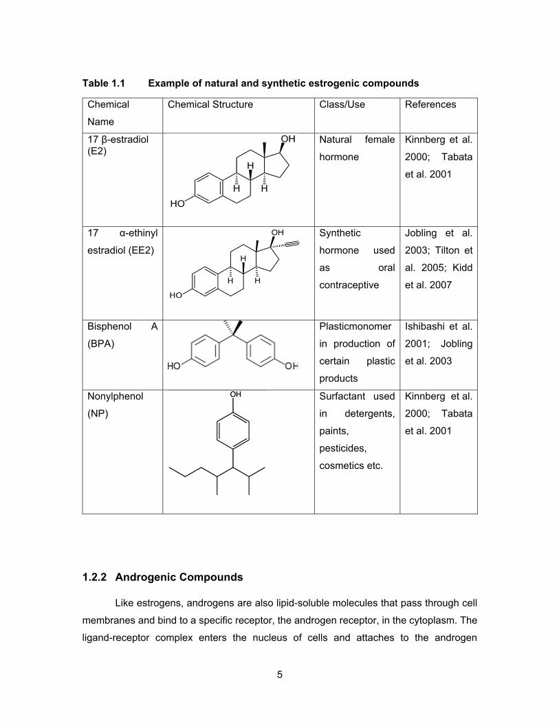
Synthetic and naturally occurring anabolic steroids are used in cattle farms to

promote growth, e.g., trenbolone acetate (Tb), testosterone, zeranol and melengestrol

acetate (MGA) (Lange et al., 2002). There has been an increased use of TBA in the cattle

industry and as a result, TBA and its metabolites have been detected in the leachate of

farms in the USA (Soto et al., 2004; Durhan et al., 2006). Studies have shown that TBA is

more potent than testosterone in terms of binding to AR in humans and fish (Bauer et al.,

2000; Ankley et al., 2003). Aquatic life exposed to anabolic steroids has shown reduction

in plasma vitellogenin levels, masculinization of female fish, reduced fecundity and

development of secondary male characteristics (Velasco-Santamaria et al., 2010; Kolok

and Sellin, 2008; Sellin et al., 2009). Table 1.2 shows some of the androgenic compounds

found in the environment.

7

Table 1.2 Example of natural and synthetic androgenic compounds

Name Chemical Structure Class/Use References Testosterone (T)

Natural hormone

Bauer et al. 2000; Damstra et al. 2002

Dihydrotestosterone (DHT)

Natural hormone

Bauer et al. 2000; Soto et al. 2004

Trenbolone (Tb)

Synthetic androgen used as anabolic steroid

Ankley et al. 2003; Seki et al. 2006; Sellin et al. 2009

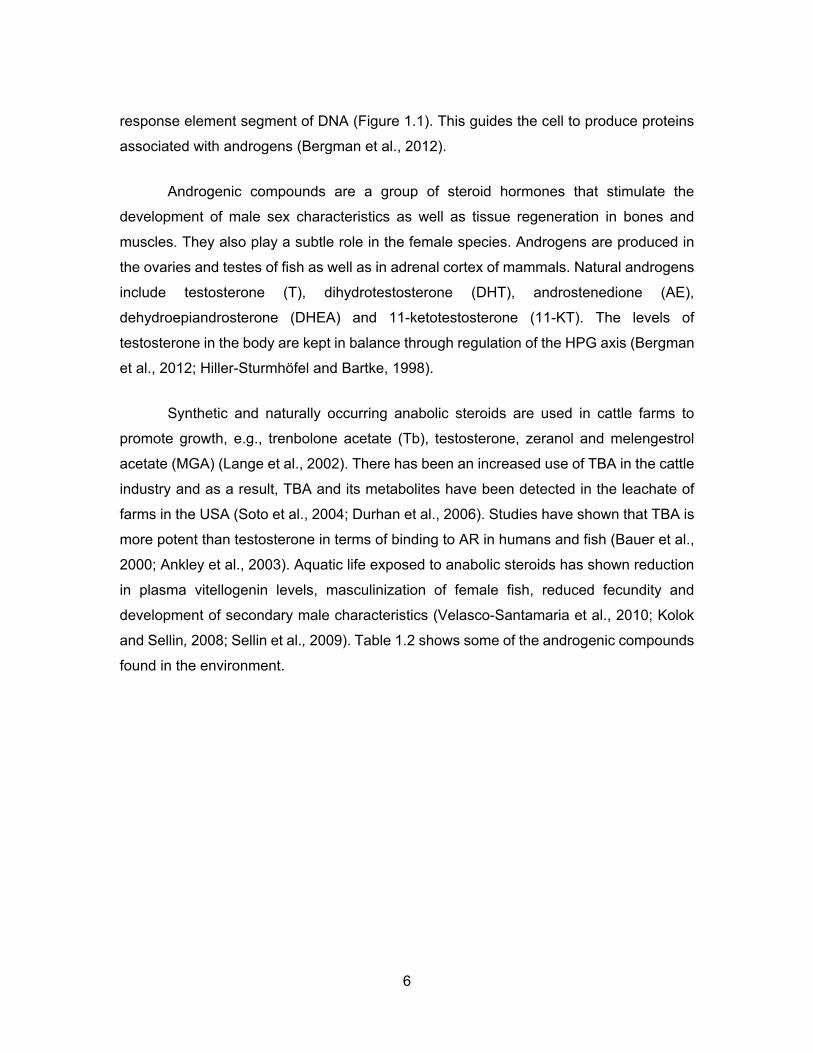
1.2.3 Glucocorticoid Compounds

Glucocorticoids are important in controlling blood glucose levels, metabolism of

carbohydrates, proteins and lipids and immune/brain functions. GCs are released from the

adrenal cortex after HPA axis activation (Damstra et al., 2002). Endogenous

glucocorticoids include cortisol, cortisone and corticosterone. Anti-inflammatory drugs that

are widely used in humans and animals include prednisone, dexamethasone,

hydrocortisone and cortisone (Iglesias et al., 2014). Table 1.3 shows some of the common

anti-inflammatory drugs used in human and veterinary medicine today.

Many anti-biotic and anti-inflammatory drugs are found in calf hutches, lagoons,

manure application and aquaculture (Watanabe et al., 2010). Glucocorticoids often are

used to induce weight gain in animals since they are found to have synergistic effect with

anabolic steroids (Reig et al., 2006). Pharmaceuticals, including GCs, have been detected

8

in lakes and other bodies of water near farmlands all over the world (Shi et al., 2013).

Cherlet et al. (2004) and Reig et al. (2006) detected dexamethasone in bovine milk and

feed of livestock. Thus, runoffs from farm fields carrying natural and synthetic drugs and

their metabolites are of concern as they can potentially cause adverse health effects in

aquatic organisms (Fent et al., 2006; Ziylan and Ince, 2011).

GCs exert their action the same way as estrogens and androgens do. They enter

the cell and bind to the glucocorticoid receptor in the cytosol. The complex then

translocates to the nucleus and binds to glucocorticoid response element (GRE), a binding

domain on DNA, to regulate gene transcription (Figure 1.1) (Bergman et al., 2012).

Table 1.3 Example of natural and synthetic glucocorticoids

Name Chemical Structure Class/Use References

Cortisol

Natural stress

hormone

Möstl et al. 1999;

Macikova et al.

2014

Cortisone

Natural stress

hormone

Möstl et al. 1999;

Iglesias et al.

2014

Dexamethasone

Synthetic

Glucocorticoid

Cherlet et al.

2004; LaLone et

al. 2012

Hydrocortisone

Natural and

synthetic

Glucocorticoid

Macikova et al.

2014

9

1.2.4 Aryl Hydrocarbon Receptor (AhR) Agonists

This group of EDC are not hormones but are aromatic hydrocarbons that can

activate the aryl hydrocarbon receptors. The majority of the AhR ligands are formed as a

result of incomplete combustion of organic materials and anthropogenic activities. These

chemicals include halogenated aromatic hydrocarbons (HAHs), polyaromatic

hydrocarbons (PAHs), polychlorinated biphenyls (PCBs), polychlorinated furans,

organochlorine pesticides (OCPs), polychlorinated dioxins and dioxins-like compounds

(Denison et al., 2002). Table 1.4 lists some of the AhR agonists in the environment. These

compounds are persistent in the environment due to chemical stability and hydrophobicity.

They are released into the environment through incineration of household and industrial

waste, as industrial by-products, and incomplete combustion of coal, diesel fuel, tar and

plant materials (Boström et al., 2002). AhR activation is usually associated with xenobiotic-

induced toxicity and carcinogenicity but it can also disrupt hormonal functions as crosstalk

between AhR and nuclear receptors has been observed (Matthews and Gustafsson,

2006).

AhR is bound to a chaperone complex in the cytoplasm. Upon binding of a ligand

to AhR, the complex translocates into the nucleus where the chaperone complex

dissociates and Ahr-ligand dimerizes with AhR nuclear translocator (ARNT). The AhR-

ARNT heterodimer binds to xenobiotic responsive elements (XRE) of the DNA and

regulates transcription of its target genes. In general these target genes encode for

biotransformation enzymes such as CYP1A1 and CYP1A2 in the CYP450 family members

(Pocar et al., 2005).

Endocrine disrupting effects through AhR activation have been reported in animals

exposed to PCBs, dioxins and PAHs. For example, whales, exposed to PCBs, were found

to have significantly low levels of thyroid hormone, thyroxine (T4) (Villanger et al., 2011).

This was due to PCBs binding to AhR and modulating (increasing) gene expression of an

enzyme involved in metabolic elimination of T4; another possible mechanism is PCBs

interfering with thyroid hormone signalling by binding to thyroid hormone transport proteins

(Kato et al., 2004). Rats dosed with 2,3,7,8-Tetrachlorodibenzo-p-dioxin (TCDD) had

premature reproductive senescence and a decrease in E2 level (Shi et al., 2007). TCDD

has been shown to lower E2 serum levels by altering steroidogenic enzymes (Takeda et

10

al., 2009). Benzo [a] pyrene (BAP) can cause a reduction in E2 and ovotoxicity in rats (Xu

et al., 2010). BAP exposed killifish have low levels of aromatase which converts

androgens into estrogens thus leading to developmental problems (Patel et al., 2006).

Table 1.4 Example of AhR agonists

Name Chemical Structure Class/Use References

Benzo [a] pyrene (BAP)

A PAH, by

product of

combustion

and a known

carcinogen

Patel et al.

2006; Xu et al.

2010

Polychlorinated Biphenyl (PCB) 28

Industrial

coolant and

plasticizer

Kato et al.

2004;

Villanger et al.

2011

2,3,7,8-

Tetrachlorodibenzo-

p-dioxin (TCDD)

Industrial

waste and

through

combustion of

fossil fuels

Shi et al.

2007; Takeda

et al. 2009

1.3 Yeast Screening Bioassays

EDCs in the environment are detected and quantified using various chemical

analyses and bioassay procedures. These include in vitro cell based assays using yeast

strains or mammalian cell lines and chemical analysis using gas chromatography-mass

spectrometry (GC-MS) or high performance liquid chromatography (HPLC). Each of these

methods has its own advantages and disadvantages in terms of specificity, sensitivity and

cost (Nie et al., 2009; Balsiger et al., 2010)

11

Yeast based reporter assays have been widely used in the detection of EDCs in

the environment samples (Chang et al., 2014; Giesy et al., 2002). Recombinant yeast cells

are transformed with a specific receptor, its response element (RE) and a reporter protein

such as β-galactosidase or luciferase. Recombinant yeast bioassays measure relative

activity of a compound without any prior knowledge about the substance’s chemistry.

Upon binding of a ligand the receptor is activated and subsequent production of reporter

protein is measured (Figure 2.5) (Campbell et al., 2006). Various studies have validated

yeast-based bioassays as a sensitive and robust screening tool for the determination of

estrogenic (Noguerol et al., 2006; Gaido et al., 1997), androgenic (Bovee et al., 2009;

Bhattacharjee and Khurana, 2014), glucocorticoid (Bovee et al., 2011; Antunes-

Fernandes et al., 2011) and aryl hydrocarbon agonists (Noguerol et al., 2006; Alnafisi et

al., 2007) activities.

1.4 Research Objectives and Study areas

The objective of the present study was to test for EDC levels in water and

sediments samples from various water bodies in British Columbia, Canada. Figure 2.1 is

the overview map of the region of the Fraser Valley where samples were collected. The

current study is the first report on the concentrations of estrogenic, androgenic,

glucocorticoid and aryl hydrocarbon agonist compounds present in these sites. The levels

for each type of EDCs were obtained using four different yeast bioassays (See Material

and Methods). Multiple samples were collected during dry and wet periods from the same

locations to assess seasonal and temporal variations in EDCs.

The study area included sloughs, a creek, rivers, canal and ditches that receive

runoff from agricultural lands containing manure and fertilizers, untreated water from a

pump station, storm sewer and compost facility. These sites were deemed at risk to

accumulate natural and synthetic compounds such as 17 β-estradiol, bisphenol A,

testosterone, trenbolone, melengestrol acetate, dihydroabietic acid and a multitude of

pesticides, herbicides and fungicides used in farms. These chemicals have the potential

12

to cause adverse effects on the aquatic life present in the sloughs, creek, rivers, canal and

ditches.

Fish kills in the tributaries in the Fraser valley have been attributed to runoff from

agricultural land (Hall and Schreier, 1996). The sampling location in Agassiz slough is

downstream from the town’s storm sewer output. Thus, the wastes from urban and rural

human population as well as runoff from dairy farms present in the vicinity of the slough

impact this site. Another site, Mountain slough, a close-by area, is also impacted by

multiple dairy and berry farms. Mountain slough is also a known laying site for Oregon

spotted frogs. This frog species has been declared endangered due to urbanization and

agricultural activities that have led to its disappearance from 78% of its former range

(USFWS, 2014). The surviving populations are in constant threat from chemicals that

wash into wetlands from farmlands (Ministry of Environment, B.C. 2002). Another two

endangered fish species, the Salish sucker and the Nooksack Dace, reside in Agassiz

Slough, Miami River and Pepin creek. Although Pepin creek has good population of fish,

they are mainly threatened by agricultural activities in the British Columbia’s Fraser Valley

(Fisheries and Oceans Canada, 2010).

The sites in Surrey were important in that discharge from the pump station, farms

(agricultural and dairy), urban/rural runoffs drain down to Nicomekl river which is home to

salmonids and non salmonids fish. Although not threatened, chronic exposure to

contaminants draining into the river can lead to bioaccumulation in fish tissues.

The purpose of the present study were to obtain and test environmental samples

from areas in the Fraser valley of British Columbia that have never been tested for these

contaminants using the yeast-based bioassays and to conduct a preliminary risk

assessment for the aquatic species in these areas.

13

2. Materials and Methods

2.1 Sampling Sites

Figure 2.1 shows the overview map of the areas (circled) of the Fraser Valley

where samples were collected. The detailed maps are followed in the sections below.

Figure 2.1 Overview map of sampling sites (circled) in Metro Vancouver and Fraser Valley of British Columbia, Canada.

2.1.1 Sampling sites in 2013

There were a total of 9 sampling sites of which 4 were from the District of Kent

(AS, MT1, MT2, MT3); 3 from the village of Harrison Hot Springs (MR1, MR2, MR3) and

2 from a creek running through the city of Abbotsford and Langley (PN1, PN2). Each site

was sampled in June, August and November for water and sediments. Due to

inaccessibility, sediments could not be collected from MR1 in November. Figures 2.2 and

2.3, and Table 2.1 provide more detailed information on these sites.

14

Figure 2.2 Sampling sites in District of Kent and Village of Harrison Hot Springs

15

Figure 2.3 Sampling sites located in Pepin Creek

16

Table 2.1 Sampling locations in 2013

Site ID &

Locations

Sampling Dates UTM

Easting Northing

Site Description

AS – Agassiz

Slough

Kent Municipality

June 19th

August 12th

November 4th

589111 5453638 Downstream of the

town’s storm sewer

output; this site is

impacted by

urban/rural

population as well

as dairy farms

MT1 – Mountain

Slough

Kent Municipality

June 19th

August 12th

November 4th

583320 5454864 Downstream of

Hogg Slough inlet

which drains

multiple dairy farms

MT2 – Mountain

Slough

Kent Municipality

June 19th

August 12th

November 4th

583251 5455096 Downstream of

Mountain Slough

inlet which drains

multiple dairy farms

and is a known

laying site for

Oregon spotted

frogs

MT3 – Mountain

Slough

Kent Municipality

June 19th

August 12th

November 4th

585656 5456787 Downstream of a

cranberry/blueberry

farm

MR1 – Miami

River

June 19th

August 12th


dairy farm

17

Harrison Hot

Springs

November 4th

MR2 – Miami

River

Harrison Hot

Springs

June 19th

August 12th

November 4th


golf course and

MR1

MR3 – Miami

River

Harrison Hot

Springs

June 19th

August 12th

November 4th

587747 5461950 This site is just

before entering

Harrison Lake; it is

impacted by the

town of Harrison

and several dairy

farms. It would

capture all

upstream

contaminants

including MR1 and

MR2.

PN1 – Pepin

Creek

Abbotsford

June 17th

August 12th

November 13th

539879 5423464 Downstream from

a permitted

compost facility

PN2 – Pepin

Creek

Langley

June 17th

August 12th

November 13th

538501 5427856 Last site before

creek enters USA,

it would capture all

upstream

contaminants

18

2.1.2 Sampling sites in 2014/15

There were 13 sites in total for the 2014/15 sampling period – all from the city of

Surrey. Each site was sampled twice, once on October 10th, 2014 and again on February

24th, 2015 except S1, S2 and S3 in October because S1 and S3 were inaccessible and

no water was found in S2. Figure 2.4 and Table 2.2 provide more detailed information

about these sites.

Figure 2.4 Sampling sites in the city of Surrey

19

Table 2.2 Sampling locations in 2014/15

Site ID UTM

Easting Northing

Site Description

S0 517755 5438618 Impacted by blueberry

farm and not connected

to any of the other study

sites

S1 517031 5439054 Collects flow from pump

station


station


station


station

S5 517576 5439029 Runoff from a blueberry

farm

S6 517746 5438666 Runoff from blueberry

farms


station and blueberry

farms

S8 517792 5437893 Could be impacted by

dairy farm

20

S9 517754 5437553 Nicomekl River site of

Salmonidae and non

salmonidae, could have

impact by dairy farm

S10 518842 5439017 Might be influenced by a

Racetrack

S11 518398 5437459 Downstream of all other

sites (except S0, S9 and

S12), last point before

entering Nikomekl River

S12 519310 5437037 In Nikomekl River, not

impacted by any other

study sites

2.2 Chemicals used in the yeast assays and chemical analyses

The standard compounds used in the yeast screen bioassays were 17β-estradiol

(E2), trenbolone (Tb), deoxycorticosterone (DOC) and β-naphthoflavone (NAP). They

were purchased from Sigma-Aldrich (Ontario, Canada). Other chemicals used in the

preparation of media were: L-histidine, L-leucine and uracil from Sigma, Difco yeast

nitrogenous base w/o amino acids and ammonium sulphate from BD Bioscience (ON,

Canada), Anhydrous dextrose from Merck Canada, galactose, synthetic complete amino

acid dropout mix minus histidine, leucine, and uracil, Tryptophan from MP Biomedicals

(OH, USA). Agar from Fisher Scientific. Methanol, acetone, ethyl acetate were from Fisher

Scientific. Empore octadecyl C18 47mm solid phase extraction disks were obtained from

Supelco Analytical (PA, USA) and Millipore 1.0 μm glass-fiber filters were from Sigma-

Aldrich.

21

Chemicals and other materials used in chemical analysis of samples included 17α-

ethynylestridiol (EE2), estriol (E3), estrone (E1), bisphenol A (BPA), nonylphenol (NP) and

internal standards β-estradiol-d3 and bisphenol A- d16, all from Sigma Aldrich (ON,

Canada). Internal standards 17β-trencolone-d3 and 5α-dihydrotestosterone-d3 were

purchased from Cerilliant (Texas, USA). Methanol (HPLC grade), acetonitrile,

dicholoromethane, acetone and isooctane were ACS reagent grades and were from

Caledon (ON, Canada). Sulphuric acid (ACS reagent) from Anachemia (QC, Canada).

Pyridine 99.8% from Sigma-Aldrich. Hexane (HPLC grade) from EMD Chemicals (NJ,

USA). Derivatization agents Bis (trimethylsiyl) trifuoroacetamide (BSTFA) with 1%

trimethylchlorosilane (TMCS) and N-methyl-N-(trimethylsilyl) trifluoroacetamide (MSTFA)

were from Sigma Aldrich.

Extraction Cartridges used were Oasis HLB (6cc, 50mg) and Sep-Pak Silica (6cc,

500 mg) from Waters Corporation (MA, USA), Agilent sampliQ C18 (6cc, 500 mg) from

Agilent Technologies (CA, USA).

2.3 Sample storage and extraction

Water was collected as grab samples by immersing the narrow, open-mouth

amber glass 1L bottle just below the surface of water. Amber glass 250 ml jar was used

to scoop the top 2-4 cm of sediments under the water while overlaying water was drained

off. After sampling, water and sediment samples were placed immediately in a cooler

containing ice. The water samples were kept at 4°C while the sediment samples were

transferred to -15°C freezer upon arrival at the laboratory and were extracted within 48 h

of collection.

Water samples were first filtered using 1.0 μm glass fiber filter to remove

particulates, then extracted according to Huang and Sedlak (2001) with modifications.

Briefly, Empore 3M C18 extraction disk (ON, Canada) was conditioned with 10 ml

methanol (MeOH) and 10 ml distilled water in sequence under the vacuum. Filtered water

sample (50 – 250 ml) was then passed through the disk. The disk was eluted with 10 ml

MeOH. The methanolic eluent was collected and evaporated down to dryness under a

22

gentle stream of nitrogen (N2). The remaining residues were reconstituted in 500 μl of

MeOH. The extract was kept in a 4°C refrigerator until used for bioassay.

Sediment samples were extracted using the liquid phase extraction method

reported by Ternes et al. (2002) with modifications. About 10-20g of sample was

transferred to a centrifuge tube containing 10 ml ethyl acetate. The tube was capped and

shaken for 10 min before being centrifuged at 1341g for 10 min. The ethyl acetate layer

on top was removed to a separate glass tube. This process was repeated twice with a

total of ~ 30 ml of ethyl acetate collected. This solution was evaporated to dryness under

a gentle stream of N2.The remaining residues were reconstituted with 500 µl of MeOH and

kept in a 4°C refrigerator until use for bioassay. Since most of the extracts from sediment

samples showed toxicity to the yeast cells, an additional silica gel cleaning step was used

to reduce the toxicity of the extract according to Bistan et al. (2011). Briefly, the residues

were reconstituted in 2 ml ethyl acetate instead of 500 µl MeOH. The silica gel cartridge

was conditioned with 2 ml MeOH and then 2ml distilled water. The ethyl acetate solution

was passed through the conditioned cartridge and the cartridge was then eluted with 10

ml acetone: ethyl acetate (5:95). This eluate was collected and evaporated to dryness.

The residues were reconstituted with 500 μl of MeOH and kept in a 4°C fridge until use for

bioassay.

2.4 Protocol for the yeast screen bioassays

The following is the theoretical basis of the yeast screen bioassays: estrogenic,

androgenic, glucocorticoid or AhR agonists are bound to the respective receptors in the

specific yeast strain causing an up regulation in the production of β-galactosidase. Upon

addition of buffer substrate mixture the yeast cells are lysed and β-galactosidase is

released in to the medium (Figure 2.5). Addition of a substrate will yield a luminescent

signal proportional to the amount of receptors activated in the yeast (Balsiger et al., 2010).

The yeast bioassays are abbreviated based on the receptor that is expressed in each e.g.

yeast estrogen screen (YES), yeast androgen screen (YAS), yeast glucocorticoid screen

(YGS) and aryl hydrocarbon receptor (AhR) assay.

Saccharomyces cerevisiae yeast cells were used for the bioassays; these had

been transformed with the human estrogen receptor (ER), the androgen receptor (AR),

23

the glucocorticoid receptor (GR) and the aryl hydrocarbon receptor (AhR) (Cox and Miller,

2002; Balsiger and Cox, 2009; Balsiger et al., 2010). All yeast cells were generously

provided by Dr. Marc Cox’s laboratory at the University of Texas, El Paso, USA. Table 2.3

lists the yeast strains, growth media and standard compounds used for each assay. For

example, for the estrogenic assay the yeast strain used was DSY-219 in the growth

medium SC-UW; SC-UW refers to synthetic complete (SC) media being prepared without

uracil (U) and tryptophan (W). Protocols for the preparation of agar plates and growth

media are provided in Appendix A.

Figure 2.5 Example of Yeast Estrogen Screen mechanism (Bazin et al., 2013 licenced under CC BY 4.0)

24

Table 2.3 Yeast strains, media and standards for the four yeast screen bioassays

Yeast assay Standard

compound

Yeast strain Growth media

Yeast estrogen

screen (YES)

17β- Estradiol DSY-219 SC-UW

Yeast androgen

screen (YAS)

Trenbolone DSY-1555 SC-LUW

Yeast

glucocorticoid

screen (YGS)

Deoxycorticosterone DSY-1345 SC-UWH

Yeast AhR binding

screen

β-Naphthoflavone MCY-038 SC-W

See Appendix A for Growth Media composition and yeast strain info. SC=synthetic complete; U=Uracil; W=Tryptophan; L=Leucine; H=Histidine

The yeast cells were stored in a -80°C freezer until ready to be grown on an agar

plate. Once yeast grew on the agar plate, it was kept at 4°C and used to run bioassays

before being discarded after one month. The yeast assay protocol was same for all four

bioassays and was adopted from Balsiger et al. (2010) with modifications. Briefly, a few

yeast cell colonies were removed from the agar plate and inoculated into 5 ml growth

media and grown overnight at 30°C. The next day, the culture was diluted with growth

media to prepare a solution with an optical density (O.D.) of 0.08 absorbance at 600 nm.

This diluted solution was incubated at 30°C until the culture reached O.D.600 of 0.1. While

culture was incubating, a 1μl aliquot of each standard (as control) and sample extract

dilution series (see Table 2.4 for concentrations used) were put into an opaque 96 well

culture plate (Fisher Scientific, USA) in triplicates. Once the OD 600 of the culture reached

25

0.1, 100 μl of culture media was added into each well of a 96 well plate. The plates were

sealed with parafilm and kept at 30°C for 2 h. At the end of the incubation period, a solution

containing 100 μl of Tropix Gal-screen buffer and substrate (Life Technologies, CA) at a

ratio of 1:24 was added into each well and mixed. The plates were covered with aluminum

foil and kept at room temperature (~22°C) for an additional 1.5-2 h. Luminescence was

measured using a Multilabel plate reader (Perkin Elmer, ON, Canada).

Table 2.4 Dilution series for each standard and test sample

Sample tested Dilution Series*

1 2 3 4 5 6 7

17β- Estradiol

(3.00E+6 ng/ml)

300 30 3 0.3 0.03 0.003 -

Trenbolone

(4.0E+3 ng/ml)

1.5 0.8 0.5 0.4 0.2 0.1 0.05

Deoxycorticosterone

(2.70E+6 ng/ml)

27 13.5 6.8 3.0 1.5 0.8 0.4

β-Naphthoflavone

(2.72E+6 ng/ml))

2720 272 27 0.27 0.027 0.0027 -

Test sample extract 1 0.5 0.1 0.01 0.001 0.0001 -

* Each concentration is in ng/ml; dilution factor was used for the test sample extract.

26

2.5 Calculation and data analysis

Concentration-response curves for the standard and sample dilution series (Table

2.4) were plotted using the Graph pad Prism 6 Software (San Diego, CA, USA) An erratic

or reversed dose-response curve indicates that the sample is non-responsive to yeast and

those samples were not included in the calculation. EC50s and slopes for the samples

were obtained from the concentration-response curves. EC30 and EC20 were calculated

from EC50 as follow:

EC30 = (0.429^(1/slope))*EC50

EC20 = (0.25^(1/slope))*EC50

The concentration equivalents (EQ) of an EDC standard in each sample was then

calculated at EC50, EC30 and EC20 using the following equation by Lorenzen et al.

(2004):

EQ at EC50 (ng/ml or g) = [Standard EC50 (ng/ml)/ Sample EC50 (unitless)] x [volume of

assay medium (ml)/ volume of extract tested(ml)] x [volume of stock extract/volume or

weight of water (ml)/sediment (g) sample]

Where, Volume of assay medium = 201μl

Volume of sample extract = 1 μl

Volume of stock extract = 500 μl

Volume of water or weight of sediment = the amount of sample extracted, i.e.,

50-250 ml for water and 10-20 g for sediment.

The final equivalents for each sample were calculated as the average of EC50,

EC30 and EC20 obtained from the equation above. Thus, the final amount represents

mean ± SEM (standard error of the mean) in ng/ml for water and ng/g dry weight for

sediments. For further data analysis, one factor ANOVA was used to determine significant

difference at p < 0.05 for temporal variations.

27

2.6 Gas chromatography-mass spectrometry analyses

Methods for the analysis of estrogenic, androgenic and AhR agonists containing

samples are followed in sections below. A ddH2O water sample spiked with standard and

deuterated internal standards were also analyzed for estrogens and androgens. For the

spiked estrogenic sample, 1 L water was spiked with E2-d3, BPA-d16, E2, EE2, E3, E1,

BPA and NP. The extraction and derivatization methods are described below in section

2.6.1. For the spiked androgenic sample, 1 L water was spiked with Tb-d3, DHT-d3, Tb

and DHT. The extraction and derivatization protocols applied to samples are described in

section 2.6.2.

2.6.1 GC-MS analysis of estrogenic compounds

Three samples with high estrogenic activity were extracted and derivatized using

the method described by Nie et al. (2009). Briefly, 1 L of water samples were acidified by

40% H2SO4 to the pH of 3. The sample was then filtered using 1.0 μm glass fiber filter.

The Oasis HLB cartridge was conditioned with 5 ml of MTBE, 5 ml of MeOH and 5 ml of

ultrapure water in sequence before the water sample was passed through at a flow rate

of 4-5 ml/min. The cartridge was then washed with 5 ml of 10% MeOH in water, 5 ml of

ultrapure water and lastly with 5 ml of 10% MeOH containing 2% NH4OH. The cartridge

was left to dry for 40 min under the vacuum.

For sample cleanup, Sep-Pak Silica cartridge was conditioned with 5 ml of

dicholoromethane/acetone (7:3 v/v) and was connected to the bottom of the Oasis

cartridge used for extraction. 10 ml of dicholoromethane/acetone (7:3 v/v) was added

through the Oasis cartridge that then passed through the Sep-Pak Silica cartridge at a

flow rate of 1-2 ml/min. The eluted liquid was evaporated under a gentle stream of N2 and

derivatized for GC-MS analysis.

The purified extract was derivatized by first dissolving the dried extract in 50 μl of

pyridine and 50 μl of Bis (trimethylsiyl) trifuoroacetamide (BSTFA) with 1%

trimethylchlorosilane (TMCS). The mixed solution was heated in a 4 L ultrasonic water

bath for 30 min. The solution was cooled to room temperature before being dried under

the stream of N2. The residues were dissolved in 100 μl of hexane for GC-MS analysis.

28

2.6.2 GC-MS analysis of androgenic compounds

Two samples with high androgenic activity were extracted using the method

described by Durhan et al. (2006). Briefly, 1 L of sample was filtered through a 1.0μm

glass fiber and then pumped at a rate of ~5ml/min through an Agilent C18 cartridge which

had been washed with 20 ml of acetonitrile and conditioned first with 20 ml of MeOH and

then 20 ml of deionized water. The cartridge was then rinsed with 20ml of 50% MeOH in

water. The column was dried under vacuum for 2 min and then eluted with 2ml of MeOH

twice. The eluents were evaporated under a stream of N2. The derivatization step was

adopted from Parker et al. (2012). Briefly, the dried residues were dissolved in 1 ml

dichloromethane and evaporated again using N2. Residues were then dissolved and

vortexed in 50μl of the derivatization reagent N-methyl-N-(trimethylsilyl) trifluoroacetamide

(MSTFA) with iodine (I2) (1.4:1000 m/v). The mixture was dried again and extracts were

reconstituted in 100μl of MSTFA. This extract was heated at 60°C for 30 min to dryness

and dissolved in 100μl of isooctane for GC-MS analysis.

2.6.3 GC-MS analysis of polyaromatic hydrocarbon compounds

Two of the samples with high activity in AhR assay, were extracted using method

by Martinez et al. (2004). First, 1L of water was filtered through 1.0μm glass fiber filter

before being passed through an Oasis SPE cartridge which had been conditioned with

5ml of ethyl acetate, 5ml of MeOH and 5ml of distilled water containing 2% MeOH in

sequence. The sample was placed under vacuum at a flow rate of ~ 5ml/min. The cartridge

was rinsed with 5ml ultrapure water, dried under the vacuum and eluted with 5ml of ethyl

acetate 5 times. The extract was evaporated using N2 and residues were reconstituted in

100 μl hexane: cyclohexane: dichloromethane (1:1:1). GC-MS detection was performed

at full scan mode to detect a wider range of unknown compounds.

2.6.4 GC-MSD conditions

The system consisted of an Agilent Technologies 6890 series Gas Chromatogram,

5973 Mass Selective Detector and a 7683B series injector. The injector temperature was

29

set a 250°C, hydrogen gas flow was kept at 0.9 ml/min. 1 μl of each sample was injected

into the GC-MSD and samples were analyzed in Selected Ion Monitoring (SIM) and scan

mode.

30

3. Results and Discussion

3.1 Standard dose-response curves for the four bioassays

Figure 3.1 Dose-response curves for the four standards used in the yeast bioassays.

* each value on the curve is based on triplicate determination at each dose

Figure 3.1 shows the dose-response curves for the standard compounds in the

four yeast bioassays. Each dot on the curve represents mean response (n=3) of that

particular dose. The concentrations on the X-axis represent the dilution series from a stock

solution as provided in Table 2.4. After determining the EC50 from the curve, EC20 values

were calculated for each compound (section 2.5) which set the limits of detection (LOD)

of the bioassay. LODs determined for the YES, YAS, YGS and AhR binding bioassays

-4 -2 0 2

-50

0

50

100

150

log [17- Estradiol ] ng/ml G

ala

cto

sid

as

e A

ctiv

ity

-1.0 -0.5 0.0

-50

0

50

100

150

log [Trenbolone] ng/ml G

ala

cto

sid

as

e A

ctiv

ity

0.0 0.5 1.0 1.5 2.0

-50

0

50

100

150

log [Deoxycorticosterone] ng/ml G

ala

cto

sid

as

e A

ctiv

ity

-4 -2 0 2 4

-50

0

50

100

150

log [- Naphthoflavone] ng/ml G

ala

cto

sid

as

e A

ctiv

ity

31

were 0.025 ng 17β-estradiol equivalents/ml, 0.20 ng trenbolone equivalents/ml, 1.5 ng

deoxycorticosterone equivalents/ml and 2.4 ng β-naphthoflavone equivalents/ml

respectively. Table 3.1 shows the EC50s obtained for each bioassay compared with the

EC50s from other studies. Balsiger et al. (2010) has reported an EC50 of 0.19 ng EEQs/ml

for E2 using the same yeast bioassay as in the present study. Sanseverion et al. (2005)

obtained EC50s of 0.12 ng EEQs/ml and 0.07 ng EEQs/ml for E2 using colorimetric and

bioluminescence yeast estrogen assays, respectively. The EC50 for trenbolone reported

by Eldridge et al. (2007) using bioluminescence androgen yeast assay is much higher

than ours at 4.87 ng trenbolone equivalents/ml. This is possibly due to BLYAS being less

sensitive than the YAS assay. Riggs et al. (2003) had EC50s ranging from 4.9-23.1 ng

DOC equivalents/ml in their GR assay. A study by Noguerol et al. (2006) showed an EC50

range of 20 – 140 ng PCBs equivalents/ml which was also higher than the 9.5 ng β-

naphthoflavone equivalents/ml EC50 of our study. Probably this was due to use of different

yeast strains and plasmids in the recombinant yeast assay (RYA).

32

Table 3.1 EC50 values for each bioassay compared to other studies

Yeast Bioassay

EC50

current study

EC50

Other studies

References

Yeast estrogen

screen (YES) 0.1 ng EEQs/ml

0.19 ng EEQs/ml

(YES)

Balsiger et al. 2010

0.12 ng EEQs/ml

(colorimetric YES);

0.07 ng EEQs/ml

(bioluminescence

YES)

Sanseverion et al.

2005

Yeast androgen

Screen (YAS)

0.3 ng TbEQs/ml 4.87 ng TbEQs/ml

(bioluminescence

YAS)

Eldridge et al. 2007

Yeast

glucocorticoid

screen (YGS)

3.0 ng DOCEQs/ml 4.9 – 23.1 ng

DOCEQs/ml (YGS)

Riggs et al. 2003

Yeast AhR binding

screen

9.5 ng NAPEQs/ml 20-140 ng PCB

EQs/ml (AhR yeast

assay)

Noguerol et al.

2006

EEQs= 17β- estradiol equivalents TbEQs= Trenbolone equivalents DOCEQs= Deoxycorticosterone equivalents NAPEQs= β- Naphthoflavone equivalents PCB= polychlorinated biphenyls

33

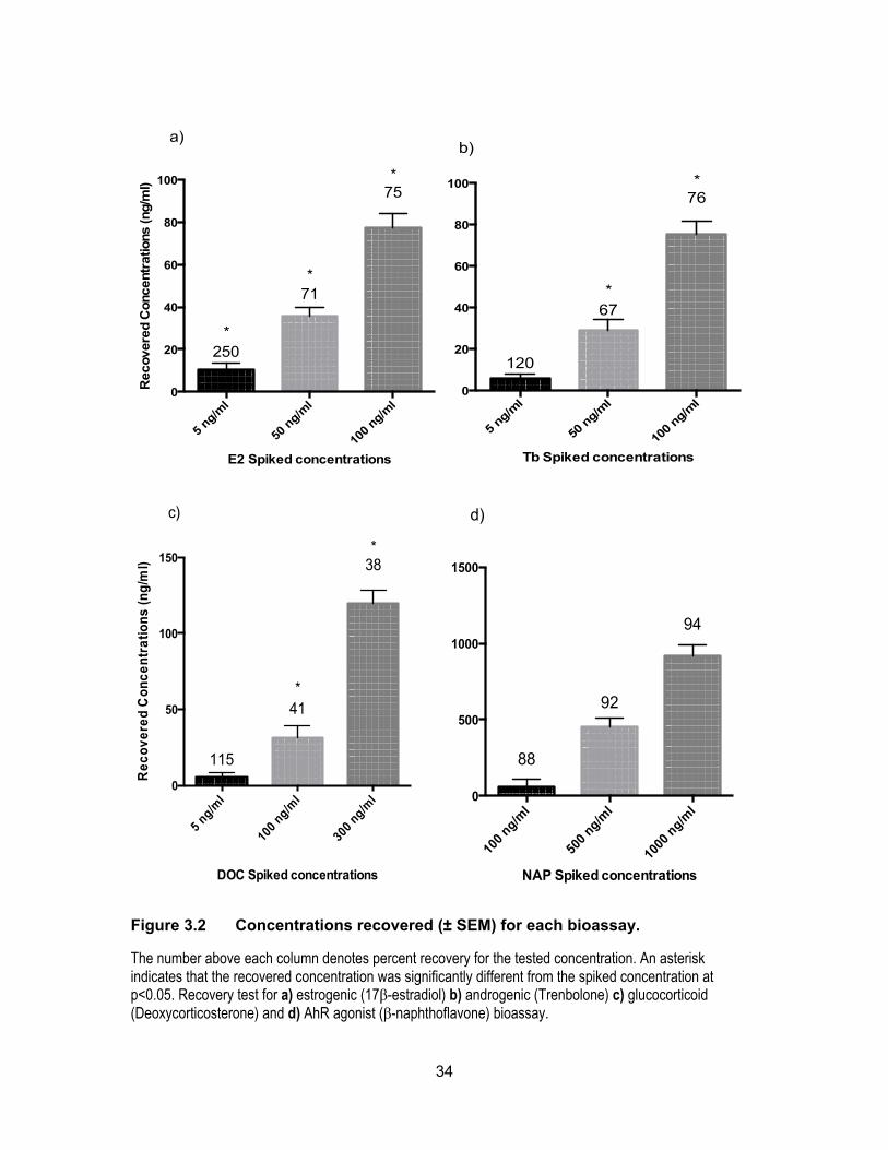
3.2 Recovery and accuracy test for the four recombinant yeast bioassays

Efficiency and accuracy of the four bioassays were examined by spiking double

distilled water with three different concentrations of the standard chemical. Figure 3.2

shows percent recoveries obtained for the four assays. For each of the spiked yeast

assays, the concentrations used were close to the levels of contamination observed in the

environmental samples. Overall, the results showed satisfactory recovery and

reproducibility for each assay except the glucocorticoid assay of which the recoveries were

only ~40%. A revised and improved extraction procedure for glucocorticoid/cortisol

compounds is necessary to obtain higher extraction recoveries for glucocorticoids.

Average percent recoveries for E2 and Tb were approximately 70% whereas NAP had the

highest accuracy and precision with recovery rates close to 92%.

34

Figure 3.2 Concentrations recovered (± SEM) for each bioassay.

The number above each column denotes percent recovery for the tested concentration. An asterisk indicates that the recovered concentration was significantly different from the spiked concentration at p<0.05. Recovery test for a) estrogenic (17β-estradiol) b) androgenic (Trenbolone) c) glucocorticoid (Deoxycorticosterone) and d) AhR agonist (β-naphthoflavone) bioassay.

5 ng/m

l

50 n

g/ml

100

ng/ml

0

20

40

60

80

100

E2 Spiked concentrations

Recovere

d C

oncentr

atio

ns (n

g/m

l)

250

71

75

*

*

*

a)

5 ng/m

l

50 n

g/ml

100

ng/ml

0

20

40

60

80

100

Tb Spiked concentrations

120

67

76

*

*

b)

5 ng/m

l

100

ng/ml

300

ng/ml

0

50

100

150

DOC Spiked concentrations

Re

co

ve

red

Co

nc

en

tra

tion

s (n

g/m

l)

115

41

38

*

*

c)

100

ng/ml

500

ng/ml

1000

ng/m

l0

500

1000

1500

NAP Spiked concentrations

94

88

92

d)

35

3.3 EDCs levels from sampling sites in 2013

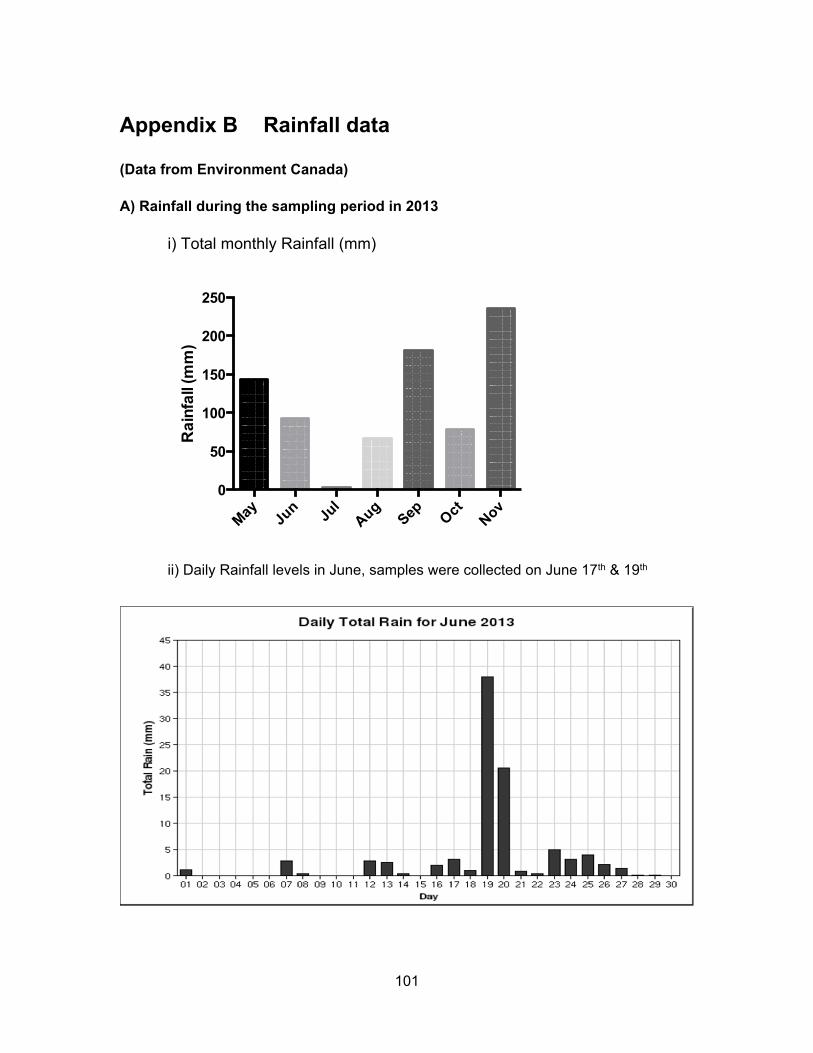
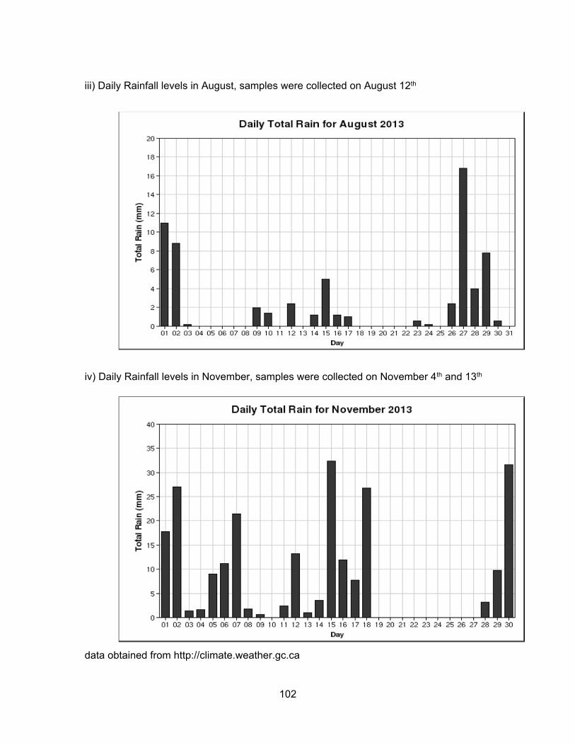
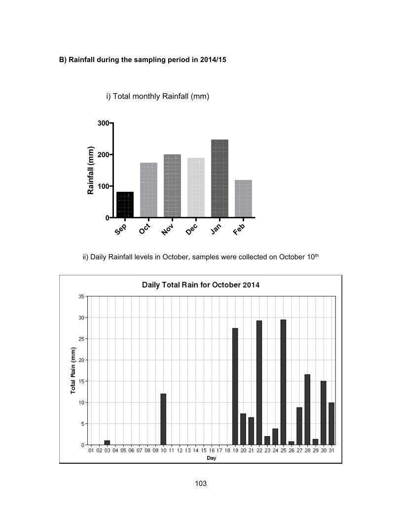
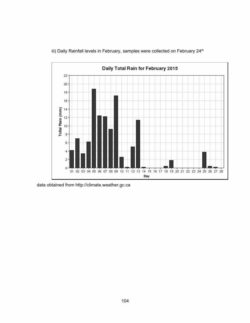
We hypothesized that rainfall levels could significantly influence the levels of

contaminants present in water and sediment. In Kent, rainfall levels were the highest in

June, lowest in August and intermediate in November. For Pepin Creek area, rainfall levels

were about the same in June and November but dry for August. Monthly and daily rainfall

levels for each location are presented in Appendix B.

3.3.1 Estrogenic levels in water and sediments

The results of the YES assay expressed as ng EEQs per ml of water and ng EEQs

per g of sediment, respectively, are presented in Table 3.2 and Figure 3.3. Figure 3.4

shows EEQs as dot sizes that are proportional to amount of estrogenic activity in water

and sediments for all sampling periods. Estrogenic activity in sediments was higher than

water for all sites in the three sampling periods, except for pepin creek sites in August

where mean water estrogenic concentrations were higher than the sediments. In the dry

period of August, four of the nine sampling sites had no detectable E2 activity in water but

the highest levels were present in sediments (3617.06 ng EEQs/ml in Miami River). Peck

et al. (2004) have reported that surface waters show very low to non-detectable estrogenic

activity but sediments are tested positively for estrogenic compounds. In terms of no

response of YES, one sediment sample from Mountain Slough (MT2) was non-responsive

in June, both water and sediments from Mountain Slough site MT3 showed no response

in November and sediments from Pepin Creek (PN2) also were non-responsive in

November (Figure 3.3).

3.3.1.1 Estrogenic levels in water

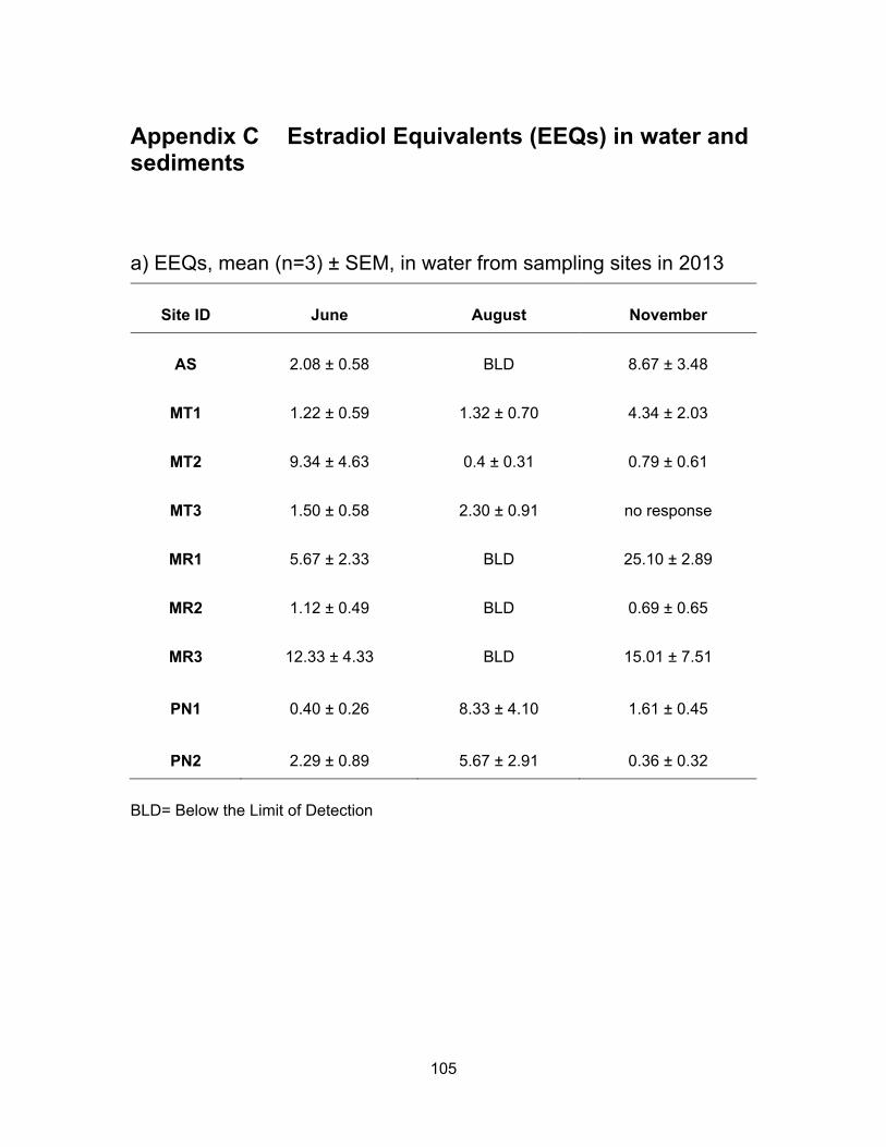
In Agassiz Slough, the mean E2 concentration in water was 2.08 ng EEQs/ml in

June, BLD in August, and 8.67 ng EEQs/ml in November. The estrogenic activity in water

was slightly higher in November compare to in June. Nonetheless, the higher levels in

both rainy periods (June and November) may reflect the impact of rain and high flow of

water bringing contaminants from dairy farms as well as urban and rural areas into the

slough.

36

In Mountain Slough locations, mean E2 activity in the water samples was about

the same in the months of June and November; about 3.90 ng EEQs/ml in both sampling

periods. E2 levels were not very different in MT1 during the three sampling periods; they

ranged from 0.31 to 2.72 ng EEQs/ml in both sampling periods of June and August and

slightly increased in November to a mean of 4.34 ng EEQs/ml. Mountain slough sites are

impacted by runoff from multiple dairy farms (MT1 and MT2) as well as berry farm and

possible chicken farm (MT3). E2 activities in MT2 water samples, except in June where it

was 9.34 ng EEQs/ml, were much lower (~ 0.60 ng EEQs/ml) compared to MT1.

November water and sediment samples from MT3 were non-responsive to bioassay, but

levels were not out of range from other Mountain Slough sites for June and August.

The three sites in Miami River showed similar pattern of E2 levels as Agassiz

slough i.e., the levels in August were the lowest, a little higher in June and highest in

November. The three different locations in Miami River, MR1, MR2 and MR3, showed the

same pattern for all three sampling periods. The river flows down from MR1 to MR2 and

into MR3 before entering Harrison Lake. MR1 is downstream of a dairy farm, the mean E2

levels in water samples were 5.67 ng EEQs /ml in June, BLD in August and went up again

after a rainfall to 25.10 ng EEQs/ml in November. MR2 is downstream of a golf course

and receives water from MR1 and dairy farms. The EEQ levels in water were BLD in

August, but mean concentrations in June and November were 1.12 and 0.69 ng EEQs/ml

respectively. The third site in Miami River, MR3 is the last spot before entering Harrison

Lake. This site would capture all upstream sources from the town of Harrison as well as

multiple dairy farms. E2 levels were BLD in August, and about the same in June and

November i.e., 12.33 and 15.01 ng EEQs/ml respectively. Our results are relatively high

compare to those reported by the study of Soto et al. (2004), of which the estrogenic

activity in river water close to cattle farms ranged from BLD to 0.99 ng EEQs/ml due

perhaps to the difference in water flows.

Unlike other locations where E2 activity was the lowest in August, the

concentrations in Pepin Creek were the highest in August with a mean value of 6.99 ng

EEQs/ml (Figure 3.3). The levels in June and November were about the same being 1.34

and 0.99 ng EEQs/ml respectively. Pepin Creek sites are impacted by a year round

compost facility and the estrogenic activity is 5x higher in August compare to June and

37

November. A year to year study would confirm if the estrogenic activity are consistently

higher in the dry period of August.

The overall pattern of a higher E2 level during rain and a lower level during dry

period is in agreement with a study by Zhao et al. (2011) in which a higher estrogenic

activity is found during wet period compare to dry period.

3.3.1.2 Estrogenic levels in sediments

Fig. 3.3 also shows the E2 concentrations in the sediment samples from Agassiz

Slough, Mountain Slough, Miami River and Pepin Creek. There were no specific patterns

of EEQ levels in the sediment samples. Some sites had similar levels in June and

November but lower in August while other sites had either higher estrogenic levels or had

no response to yeast cells in November than in the other two sampling periods. Sediment

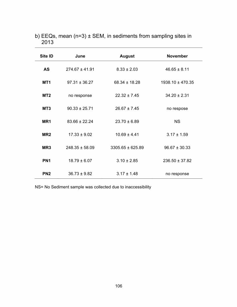
samples from Agassiz Slough had mean E2 equivalence of 274.67 ng EEQs/g in June,

8.33 ng EEQ/g in August and 46.65 ng EEQs/g in November (Table 3.2). The significantly

higher levels in June than November may be due to the heavy rainfall which preceded the

sampling day and had brought with it contaminated soils as this site also receives water

from the city’s storm sewer. Higher levels in both rainy periods may also be due to runoff

from sources further away from the sampling sites.

Sediment E2 levels in Mountain slough showed a somewhat similar pattern in June

and August but they were higher in November. These sites are impacted by multiple dairy,

chicken and/or berry farms. Mean EEQs were 97.31 ng EEQs/g in June, 68.34 in August

and 1938.10 in November for MT1. MT2 June’s samples were non responsive to yeast

(water data showed EEQs of 9.34 ng/ml), in August the levels were 22.32 ng EEQs/g and

November was 34.20 ng EEQs/g. The MT3 location had mean E2 equivalents of 90.33 ng

EEQs/g and 26.67 ng EEQs/g in June and August respectively. Sediment samples in

November were non responsive to yeast and so did the water sample.

For sediment samples from Miami River, the levels were low in November but high

in June with the exception of MR3 where the level was the highest and reached 4198.34

ng EEQs/g in August. The high E2 activity could be due to the type of clay or organic

matter in the sample as estrogenic compounds are likely to adsorb onto the sediments

(Wang et al., 2012). MR1, the most upstream location, had a mean EEQ of 83.66 ng/g in

38

June but a lower value, 23.70 ng/g in August. No sediment sample was collected in

November. For MR2, downstream from MR1, the mean E2 levels were 17.33 ng EEQs/g

in June, 10.69 ng EEQs/g in August and 3.17 ng EEQs/g in November. The last site MR3

which is downstream to the other two sites and also the last point of the river before

entering Harrison Lake, had mean E2 levels of 248.35 ng EEQs/g in June, 3305.65 in

August and 96.67 in November. The very high levels in August for MR3 could be due to

settling down of soil and sediments from upstream and due to dry weather or no flow of

water in the area leading to accumulation in sediments.

The two sites in Pepin creek had low sediment EEQs in August whereas the EEQs

were the highest in water for August. Low levels in sediments may be due to estrogenic

compound degradation as a result of warm temperatures (Tiryaki and Temur, 2010). PN1,

which is impacted by a discharge from a year round compost facility, has mean EEQs of

18.79 ng/g in June, 3.10 ng/g in August and significantly higher activity (p < 0.05) at 236.50

ng EEQs/g in November. November sediment samples from PN2, which is downstream

of PN1, did not respond to yeast. In August, the mean EEQ was not significantly different

(p < 0.05) in PN2 (3.17 ng EEQs/g) compared to PN1and higher than PN1 concentration

in June being 36.73 ng EEQs/g. The high levels could be due to water flow and

accumulation of estrogenic compounds from PN1 down to PN2. On its way the

contaminants may have accumulated as they run through a Regional park. High activity

observed downstream of the park may also be due to pesticide uses as some pesticides

have the ability to bind to estrogenic receptors (Kojima et al., 2010; Noguerol et al., 2006).

39

Table 3.2 Summary of estrogenic levels in water and sediments from Agassiz Slough, Mountain Slough, Miami River and Pepin Creek.

Sampling

Period

Sample

Type*

Agassiz Slough (AS)

L H M

Mountain Slough (MT)

L H M

Miami River (MR)

L H M

Pepin Creek (PN)

L H M

June

water 1 3 2 0.3 17 4 0.3 20 6 0.05 4 1

sediment 199 344 275 44 165 93 3 345 149 8 54 31

August

water BLD BLD 4 1 BLD 1.0 16 7

sediment 5 12 8 8 98 39 3 3617 980 0.03 9 3

November

water 3 15 9 0.06 8 4 BLD 29 14 0.02 3 0.8

sediment 33 62 47 30 2772 986 0.5 148 50 171 301 237

*Concentrations in water and sediment are presented in ng EEQs/ml and ng EEQs/g respectively. L=Low, H=High, M=Mean. Note the values are rounded to the nearest whole number.

40

Figure 3.3. YES results for Agassiz Slough (AS), Mountain Slough (MT), Miami River (MR) and Pepin Creek (PN).

+ indicates no response to yeast; black bars=water values in ng/ml, grey bars=sediment values in ng/g

ASM

T1M

T2M

T3M

R1M

R2M

R3PN1PN2

ASM

T1M

T2M

T3M

R1M

R2M

R3PN1PN2

ASM

T1M

T2M

T3M

R1M

R2M

R3PN1PN2

0.00

0.05

0.10

10

20

30

40

100

1100

2100

3100

4100

August November

E2

eq

uiv

ale

nts

in n

g/ (

ml o

r g

)

+ ++ ++

June

41

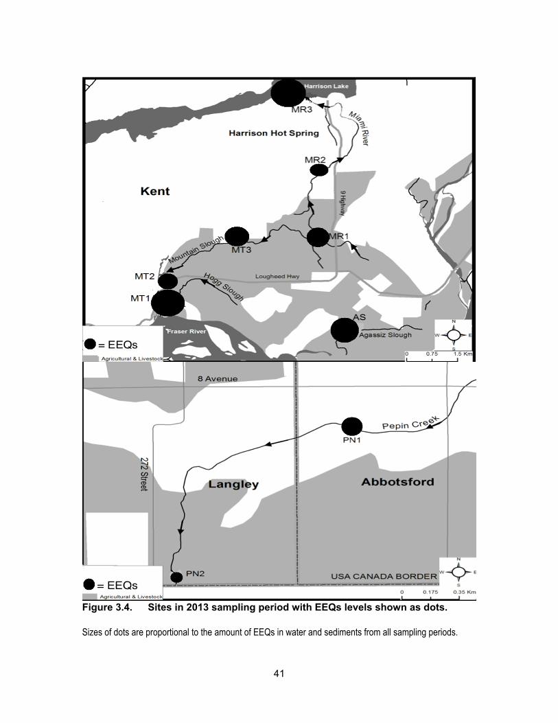
Figure 3.4. Sites in 2013 sampling period with EEQs levels shown as dots. Sizes of dots are proportional to the amount of EEQs in water and sediments from all sampling periods.

42

3.3.2 Androgenic levels in water and sediments

Results of the YAS assay are presented in Table 3.3 and Figure 3.5. Figure 3.6

shows TbEQs as dots of sizes that are proportional to amount of androgenic activity in

water and sediments for all sampling periods. Androgenic activity in the water and

sediment samples was expressed in ng trenbolone equivalents (TbEQs) per ml or g of

sample. While non of the water samples were non-responsive to yeast in the three

sampling period, there were three sediment samples that had no response which were

from different sites; two in August were from Mountain Slough and Miami River and one

in November was from Mountain Slough.

3.3.2.1 Androgenic levels in water

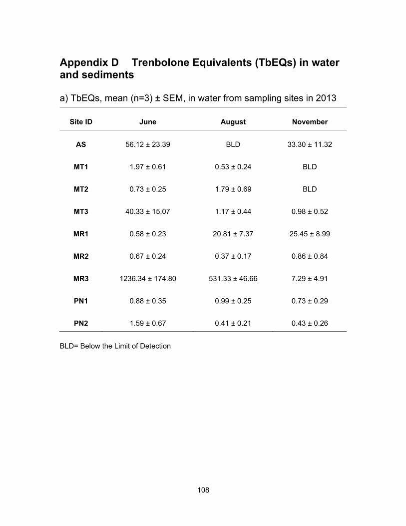
The site in Agassiz Slough, which is impacted by dairy farms as well as urban

areas, showed mean TbEQs in water of 56.12 ng TbEQs/ml and 33.30 ng TbEQs/ml in

June and November respectively but levels were below the limit of detection in August.

The undetectable levels in the dry period of August could be due to high temperatures in

the slough causing microbial degradation of androgenic compounds (Nichols et al., 1997).

The three sites in Mountain Slough, MT1, MT2 and MT3 showed low TbEQs in

water during all three sampling periods, ranging from BLD to 3.11 ng TbEQs/ml, with the

exception of MT3 having high Tb equivalents in June, up to 65.21 ng TbEQs/ml (Table

3.3). Chicken and berry farm’s influence water in MT3 and flushing of fertilizer and animal

waste is due to heavy rain in June which could explain this high levels.

Site MR3 in Miami River showed highest average androgenic activity in June

(1236.34 ng TbEQs/ml) and August (531.33 ng TbEQs/ml) compared to all the sites in

three sampling period. But Androgenic concentrations were lower in November (7.29 ng

TbEQs/ml). Tb equivalents were lower (0.58 ng TbEQs/ml) in June and somewhat same

in August (20.81 ng TbEQs/ml) and November (25.45 ng TbEQs/ml) for MR1 which is

upstream of MR2 and MR3. MR2 had similar levels in all three periods of sampling, 0.67,

0.37 and 0.86 ng TbEQs/ml in June, August and November respectively. High levels in

MR3 could be due to this site being the last point of Miami River thus collecting everything

being washed down the river from agricultural and urban land use in the area of Harrison

Hot Springs. Low levels observed in the two river sites could be due to high flow rate of

43

river flushing all the contaminants downstream that’s why the lowest point in the river had

the highest levels of androgenic activity.

Tb equivalents in Pepin creek were not significantly different (p < 0.05) from each

other (PN1 vs. PN2) and also not significantly different (p < 0.05) in the three rounds of

sampling periods (Figure 3.5). Mean TbEQs/ml were 0.88, 0.99 and 0.73 in PN1 for June,

August and November respectively. For PN2 the highest concentration was in June of

1.59 ng TbEQs/ml and dropping to 0.41 ng TbEQs/ml and 0.43 ng TbEQs/ml in August

and November respectively.

3.3.2.2 Androgenic levels in sediments

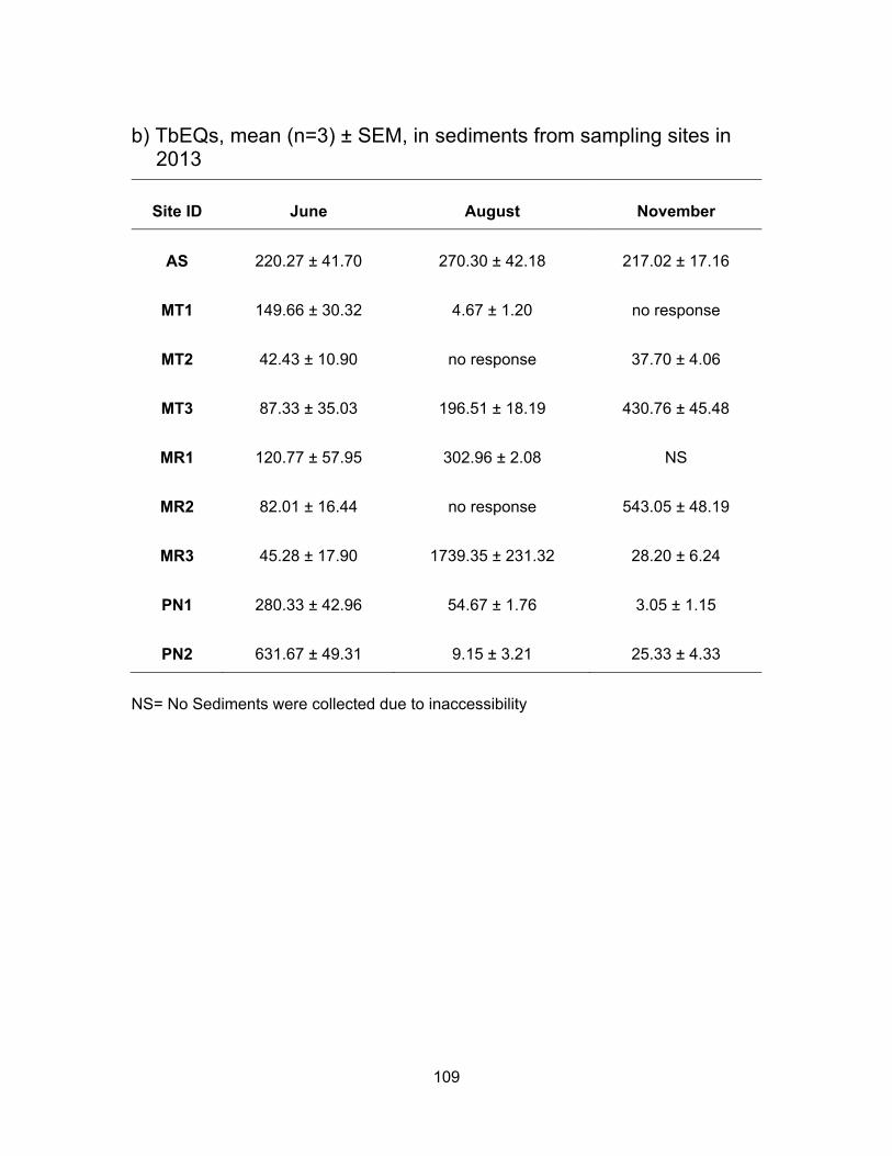
Fig. 3.4 shows Tb concentrations in the sediment samples from Agassiz Slough,

Mountain Slough, Miami River and Pepin Creek. Sediment androgenic levels were higher

than water for all sampling sites except MR3 in June when the sediment concentration

was 44.28 TbEQs ng/g compared to 1236.34 TbEQs ng/ml in water. Androgenic levels in

sediments from Agassiz Slough were about the same for the three sampling periods, with

mean values of 220.27, 270.30 and 217.02 ng TbEQs/g in June, August and November

respectively. Slightly higher levels in August could be due to accumulation of androgenic

compounds in soil which could not be washed away with water as there was only 3.4 mm

of rain leading up to the sampling date in August.

The concentration of androgenic compounds in Mountain Slough were in the range

of 21 – 203 ng TbEQ/g in June, 1 – 228 ng TbEQs/g in August, and 31 – 498 ng TbEQs/g

in November (Table 3.3). Androgenic concentration in MT1 was higher in June (149.66 ng

TbEQs/g) than in August (4.67 ng TbEQs/g) and there was no response to yeast in

November. In MT2 the levels were 42.43 ng TbEQs/g in June, and 37.70 ng TbEQs/g in

November. The sediments showed no response to yeast in August. Lower activity in dry

period possibly is due to increases in ambient temperature, light degradation of

androgenic compounds and microbial degradation (Nichols et al., 1997). MT3 showed

high levels of contamination in August (TbEQs of 196.51 ng/g) and November (TbEQs of

430.76 ng/g) compared to the other two Mountain Slough locations.

Miami River sites had TbEQs in the range of 13 – 255 ng TbEQs/g in June, 298 –

2010 ng TbEQs/g in August and 13 – 592 ng TbEQs/g in November. The lowest

44

androgenic levels were in June, about 3-5x higher in November and the highest in August.

For MR1, the levels were higher in August (302.96 ng TbEQs/g) compared to June (120.77

ng TbEQs/g) and no sediments were collected in November due to inaccessibility. For

MR2, the sediments were non-responsive in August and the levels were 82.01 ng

TbEQs/g in June and 543.05 ng TbEQs/g in November. The last site in Miami River, MR3,

the levels were lowest in June (45.28 ng TbEQs/g) and November (28.20 ng TbEQs/g)

but reached about 2010.09 ng TbEQs/g in August. The very high sediment contamination

may be because of accumulation of compounds due to a higher rate of growth hormone

use in cattle farms (Lange et al., 2002).

Androgenic activities in sediment samples from Pepin Creek were significantly

different at p < 0.05 among the three sampling periods and between the two sites PN1

and PN2 (Figure 3.5). Average TbEQs in PN1 were found to be 280.33, 54.67 and only

3.05 ng TbEQs/g in June, August and November respectively. The highest activity in PN2

was also in the rainy month of June at 631.67 ng TbEQs/g. The average concentrations

dropped to 9.15 ng TbEQs/g in the dry month of August but rose up again to 25.33 ng

TbEQs/g. Highest concentration in PN2 in the raining period of June could be due to

flowing of substances down the creek and reaching PN2 from PN1 which collects drainage

from a compost facility. The highest levels of androgenic compounds in August at PN1

can be explained by the influence of dry period where there was no washing down of

substances down the creek as compared to the raining period of June.

More detectable and/or higher levels in a rainy period are in line with the study by

Finlay-Moore et al. (2000) where high concentrations of estrogens and testosterones were

reported in both water and soil near agricultural and dairy farm lands. Whereas low

androgenic activities observed in some of the sites could be due to anti-androgenic

compounds such as PAHs, which may be present in the pesticides, used in the

surrounding farmlands.

45

Table 3.3 Summary of androgenic levels in water and sediments from Agassiz Slough, Mountain Slough, Miami River and Pepin Creek.

Sampling

Period

Sample

Type*

Agassiz Slough (AS)

L H M


L H M

Miami River (MR)

L H M

Pepin Creek (PN)

L H M

June

water 16 97 56 0.3 65 14 0.2 1577 408 0.3 3 1

sediment 154 299 220 21 203 94 13 255 87 199 709 456

August

water BLD 0.2 3 1 0.2 616 184 0.1 1 0.7

sediment 199 345 270 1 228 101 298 2010 1022 4 58 33

November

water 15 53 33 BLD 2 1 0.2 43 12 0.1 1 0.5

sediment 196 251 217 31 498 234 13 592 274 1 33 14

*Concentrations in water and sediment are presented in ng TbEQs/ml and ng TbEQs/g respectively. L=Low, H=High, M=Mean. Note the values are rounded to the nearest whole number.

46

Figure 3.5 YAS assay results for Agassiz Slough (AS), Mountain Slough (MT), Miami River (MR) and Pepin Creek (PN).


ASM

T1M

T2M

T3MR1MR2MR3PN1PN2

ASM

T1M

T2M

T3MR1MR2MR3PN1PN2

ASM

T1M

T2M

T3MR1MR2MR3PN1PN2

0

2

4

50

300

550

1200

1700

2200

June August November

Tb e

quiv

ale

nts

in n

g/ (

ml o

r g)

++ +

47

Figure 3.6 Sites in 2013 sampling period with TbEQs levels shown as dots.

Sizes of dots are proportional to the amount of TbEQs in water and sediments from all sampling periods.

48

3.3.3 Glucocorticoid levels in water and sediments

The results of the YGS assay are presented in Table 3.4 and Figure 3.7. Figure

3.8 shows DOCEQs as dots of sizes that are proportional to amount of glucocorticoid

activity in water and sediments for all sampling periods. Glucocorticoid levels in water and

sediment samples were expressed in ng of deoxycorticosterone equivalents (DOCEQs)

per ml or g of sample. Glucocorticoid assay showed the highest activity when compared

to YES and YAS and the number of samples found to be non-responsive to yeast was

also higher than in any of the other three bioassays. Our results are in agreement with

study by Van Der Linden et al. (2008), in which the highest levels detected were from

glucocorticoids compared to other EDCs such as E2, progesterone and DHT in surface

water.

3.3.3.1 Glucocorticoid levels in water

Water samples from Agassiz Slough in June and August were non-responsive to

the yeasts; the mean concentration in water was 11.13 ng DOCEQs/ml in November.

Glucocorticoid levels in Mountain Slough sites were higher compared to Agassiz Slough.

There was an increase in glucocorticoid levels with time i.e., the levels increased from

June to August and from August to November for the two Mountain Slough sites MT1 and

MT2. In MT3 the concentrations decreased in August but were the highest among all three

Mountain Slough locations in November being at 8209.77 ng DOCEQs/ml. The average

concentrations in Mountain Slough were 32.34, 461.42 and 3741.06 ng DOCEQs/ml in

June, August and November respectively. Multiple dairy and berry farms impact all three

sites in Mountain Slough. The high levels in November reflect the accumulation of

Glucocorticoid compounds in these locations over time. As reported in a study by De

Clercq et al. (2014), natural and synthetic glucocorticoids remain stable in animal excreta

and show no significant loss in the environment.

Glucocorticoid activities in Miami River were high in August and November

compared to in June (Table 3.4). MR1 the most upstream site had DOCEQs at 110.20,

7258.35 and 1553.09 ng/ml in June, August and November respectively. Low levels in

June could be due to heavy rain fall period which washed away most of the compounds

downstream. Whereas in the dry period of August, more compounds could be detected in

still water. In November the rainfall levels were moderate. In MR2, the site downstream of

49

MR1 had mean concentrations at 24.25, 28.04 and 1377.65 ng DOCEQs/ml in June,

August and November respectively. This site is downstream of a golf course. The last spot

at Miami River, MR3 had undetectable levels of glucocorticoids in June and August but

levels were not significantly different from other two Miami River location in November, as

1045.61 ng DOCEQs/ml of activity was detected in November. Low levels in June and

August may be due to dilution of water. High levels in the two sites close to dairy farms

and agricultural lands possibly be due to use of anti inflammatory drugs in animals leading

to the release of cortisol in animal excreta reaching waterways. Courtheyn and

Vercammen (1994) demonstrated that residues of corticosteroid were detectable in urine

and feces of cattle treated with dexamethasone which becomes part of runoff from

farmlands.

Water samples from PN1 had undetectable levels of glucocorticoid activities in

June and August and showed mean DOC equivalents of 9.80 ng/ml in November.

Samples from PN2 were non-responsive to yeast in June and August but were high at

749.73 ng DOCEQs/ml. No response in June and August samples from PN2 could be due

to high contamination during the time of sampling. It is interesting to note that the incidence

of sample’ no response and high levels were observed in site downstream of PN1 but not

in PN1. The contributing factor seems to be the impact from Aldergrove Regional Park

that also has horse trails and it is popular with horseback riders. Alexander & Irvine (1998)

have reported that social stress in horses causes an increase in free cortisol excretion.

3.3.3.2 Glucocorticoid levels in sediments

For sediment levels of cortisol-like chemicals (Figure 3.7, Table 3.4), there were

no results from Agassiz Slough for June and August as the samples showed no response

to yeast as did the water samples did for the same sampling period. This could be due to

high levels of contaminants present in the slough during the time of sampling. The mean

glucocorticoid levels in November were 233.20 ng DOCEQs/g. Sediment samples from

the Mountain Slough sites also caused yeast cells death. Non-responsiveness was

observed in samples from MT2 and MT3 in June and MT1 and MT2 in November. Thus

only one DOCEQs value is available from Mountain Slough from June which was 215.28

ng/g at MT1, and was not significantly different (p < 0.05) from a site in a neighbouring

Agassiz Sough. The mean concentrations reached 10,010.13 ng DOCEQs/g in August for

50

MT1. In August the mean DOCEQs for MT2 and MT3 were 17,200.42 and 1933.32 ng/g

respectively. Only one DOCEQ value is available from Mountain Slough in November from

MT3, which was 8176.98 ng DOCEQs/g which was very close to the water levels of

8209.77 ng DOCEQs/ml from the same location. Very high levels in the dry period may

be due to an increase use of anti inflammatory drugs in cattle/dairy farms or mixing of anti

inflammatory drugs with growth hormones during the period before sampling (Huetos et

al., 1999).

Levels in Miami River were the highest at the most downstream site of MR3

compared to upstream locations of MR1 and MR2. This is due to the site is downstream

of urban development as glucocorticoid drug uses by humans also discharge

glucocorticoid-like chemicals through urine and feces. The mean DOCEQs increased from

256.96 to 2227.80 to 7902.15 ng/g in June going from upstream to downstream.

Sediments were non-responsive to yeasts in August from MR1, but the levels increased

from 31.11 and 557.74 ng DOCEQs/g, respectively for MR2 and MR3. In November there

were no sediments data from MR1, but MR2 and MR3 showed the same pattern of

increased levels from the earlier months as well as increased levels as we moved

downstream of the river; levels in MR2 were 637.59 ng DOCEQs/g and in MR3 were

7455.67 ng DOCEQs/g.

Both sediment samples from Pepin creek were non-responsive in June (Table 3.4).

The average levels were measured at 111.14 and 517.80 ng DOCEQs/g in August for

PN1 and PN2 respectively. In November the mean DOCEQs at PN1 was 2999.89 ng/g

whereas samples from PN2 were non-responsive.

51

Table 3.4 Summary of glucocorticoid levels in water and sediments from Agassiz Slough, Mountain Slough, Miami River and Pepin Creek.

Sampling

Period

Sample

Type*

Agassiz Slough (AS)

L H M


L H M

Miami River (MR)

L H M

Pepin Creek (PN)

L H M

June

water no response 4 76 32 BLD 145 67 BLD/ no response

sediment no response 134 278 215 201 9207 3462 no response

August

water no response 4 3618 461 BLD 7981 3640 BLD/ no response

sediment no response 1900 18988 9711 21 736 295 89 621 355

November

water 3 27 11 1345 8999 3740 864 2098 1326 0.3 799 329

sediment 143 313 233 6895 9005 8210 567 9631 4047 2789 3211 3000

*Concentrations in water and sediment are presented in ng DOCEQ/ml and ng DOCEQ/g respectively. L=Low, H=High, M=Mean. Note the values are rounded to the nearest whole number.

52

Figure 3.7 YGS assay results for Agassiz Slough (AS), Mountain Slough (MT), Miami River (MR) and Pepin Creek (PN).

+ indicates no response to yeast; black bars=water values in ng/ml, grey bars=sediment values in ng

ASM

T1M

T2M

T3M

R1M

R2M

R3PN1PN2

ASM

T1M

T2M

T3M

R1M

R2M

R3PN1PN2

ASM

T1M

T2M

T3M

R1M

R2M

R3PN1PN2

0

50

100

5000

10000

17000

18000

19000

DOC e

quiv

ale

nts

in n

g/ (

ml o

r g)

August NovemberJune

++ ++ +++ ++ + + + + +

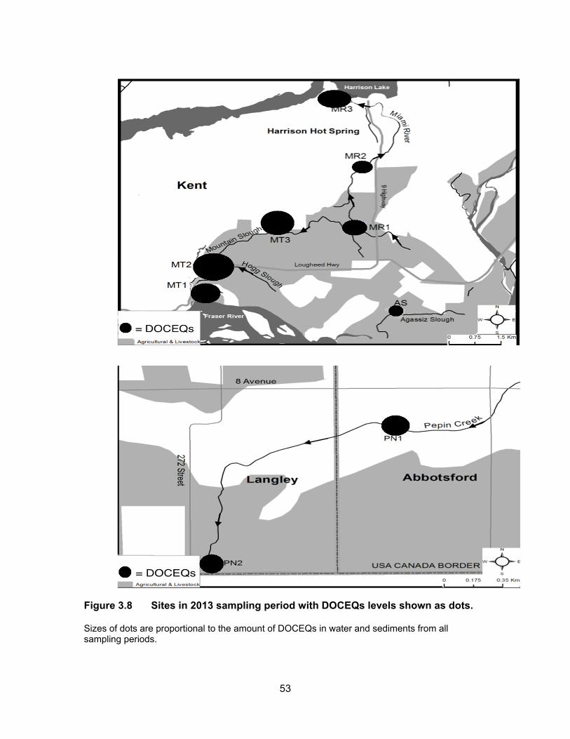
53

Figure 3.8 Sites in 2013 sampling period with DOCEQs levels shown as dots. Sizes of dots are proportional to the amount of DOCEQs in water and sediments from all sampling periods.

54

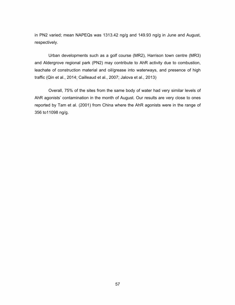
3.3.4 Aryl hydrocarbon receptor agonists levels in water and sediments

Results of the AhR binding assay expressed as ng of β-naphthoflavone

equivalents (NAPEQs) per ml or g sample of water and sediment respectively, are

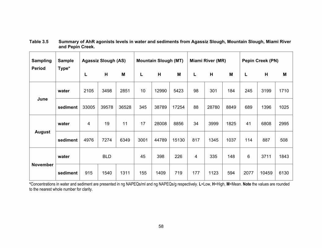
presented in Table 3.5 and Figure 3.9. Figure 3.10 shows NAPEQs as dots of sizes that

are proportional to amount of AhR activity in water and sediments for all sampling periods.

The NAPEQ levels dropped in November and were the highest in June with the exception

of a few sites. June was also the wettest month and it was expected to see a higher AhR

activity after rainfall. There was only one site, MT2, which was non responsive to yeast in

November.

3.3.4.1 AhR agonists levels in water

AhR agonists’ levels in water samples from Agassiz Slough were the highest in

June (mean NAPEQs of 2849.80 ng/ml), dropped to 11.12 ng NAPEQs/ml in August and

were undetectable in November. The M1 site in Mountain Slough had the same pattern

of the highest mean concentrations in June (5182.65 ng NAPEQs/ml), dropping in August

(1014.03 ng NAPEQs/ml) and the lowest were calculated in November (95.66 ng

NAPEQs/ml). MT2 had the same pattern of the highest levels of 11048.32 ng NAPEQs/ml

in June, dropping to very low 28.67 ng NAPEQs/ml in August and November but these

samples were non responsive to the yeasts so it could not be confirmed if it followed the

same pattern of lowest activities in November just like AS and MT1. Concentrations in

MT3 were the highest in August of 25,825.33 ng NAPEQs/ml, 356.71 ng NAPEQs/ml in

November and lowest in June of 39.01 ng NAPEQs/ml. The highest levels in August for

MT3 is supported by findings by Qin et al. (2014) of which the highest level of PAHs are

detected in summer months near agricultural lands. This may be due to increased

solubility of PAHs in higher temperatures along with water evaporation leading to

concentrated PAHs in surface water.

Levels in Miami River were about the same for the three sites in June, 156.59 ng

NAPEQs/ml in MR1 and 149.30 ng NAPEQs/ml in MR2 but slightly higher at 245.03 ng

NAPEQs/ml in MR3 (Figure 3.9). However MR3 is affected by urban development and

impact by urbanization on MR1 and MR2 is small. The concentrations of aromatic

hydrocarbon-like chemicals were higher in August at MR1 and MR2 being at 1849.11 ng

55

NAPEQs/ml and 3579.24 ng NAPEQs/ml respectively. But concentrations decreased in

MR3 to 47.30 ng/ml. During the last sampling period in November, the AhR agonists’ levels

MR3 dropped even further down to 6.28 ng NAPEQs/ml, whereas levels were 165.30 and

274.41 ng NAPEQs/ml in MR1 and MR2 respectively. Comparison of NAP equivalents in

water from June to August to November reveal that activities went from high to low from

June to November in the two Sloughs with the exception of one site, MT3. On the other

hand activities in the river were highest in August possibly due to water evaporation

causing an increase in the concentration of PAHs. Also, an increase in temperature

increased the solubility of AhR agonists in water (Qin et al., 2014). Contamination levels

are about the same in June and November, with the exception of MR3 which is the last

location in the river before Miami River enters Harrison Lake, where the levels are very

low ranging from 4.10 – 247.55 ng NAPEQs/ml. The lowest levels in MR3 may be due to

dilution of the compounds in the river and also PAHs being settled down in sediments

along the way to entering Harrison Lake.

Pepin Creek data clearly show that urban impact increases AhR agonists in the

environment as NAP equivalents are 10 to 200 times higher in PN2 compared to PN1 in

all three sampling periods (Figure 3.9). AhR agonists’ levels in PN1 were highest in June

(286.67 ng NAPEQs/ml), dropped to 57.64 ng NAPEQs/ml in August and were lowest in

November (17.19 ng NAPEQ/ml). This site has the same pattern of high and low levels at

a given sampling period as site AS, MT1 and MR3. PN2 is impacted by the Aldergrove

Regional Park, thus has influence of urbanization. The park has horse and cycling trails

as well. The highest concentrations in PN2 were in August at 5336.33 ng NAPEQs/ml,

lower in November of 3671.23 ng NAPEQs/ml and lowest at 3110.55 ng NAPEQs/ml in

June. The lowest levels in the raining period of June and November could be due to an

increase in water level in the creek and the dilution of AhR agonists.

3.3.4.2 AhR agonists levels in sediments

Fig. 3.9 shows the concentrations of NAP equivalents in sediment samples from

Agassiz Slough, Mountain Slough, Miami River and Pepin Creek. Only 19% of the

sediment samples had lower levels of NAP activity compared to the water samples from

the same location. Detection of a higher level of NAP-like contaminants in sediments is

due to preferential adsorption of hydrocarbons onto soil particles rather than being

56

dissolved in water (Hiller et al., 2008). Average NAP concentration activities in Agassiz

Slough were 36,525.91 ng NAPEQs/g in June, dropped to 6357.88 ng NAPEQs/g in

August, and dropped further in November to 1311.72 ng NAPEQs/g. These levels were

significantly different (p < 0.05) from each other. This is the same pattern we observe for

NAP concentrations in the water samples where activities decreased with time. In

Mountain Slough the levels were the highest in MT3 which was impacted by poultry and

berry farms. This may be due to the solvents used to apply pesticide and/or herbicide to

the fields, as residues of pesticides are found in wash water from farms and this could

increase the AhR activity in the waterways (Atwater et al., 1998). Activities in MT3

sediments were 34451.15 ng NAPEQs/g in June, this is comparable to levels in Agassiz

Slough in the same month. Levels in August rose to average NAPEQs of 38,263.40 ng/g

but dropped in November to 1236.22 ng NAPEQs/g. The low activity in November could

be the result of selection of sediments from a site a little further away from the farm. The

NAPEQs for the other two Mountain Slough sites were not significantly different from each

other in August, being 3750.05 ng NAPEQs/g for MT1 and 3779.05 ng NAPEQs/g for

MT2. MT had lowest levels at 203.12 ng NAPEQs/g in November and also low at 662.50

ng NAPEQs/g in June. On the other hand levels in MT2 were high at 16,648.83 ng

NAPEQ/g in June and sediments were non responsive to yeast in November which was

the case with water during the same sampling period. Overall highest levels in MT3 in all

sampling periods suggest influence of an abundance use of pesticides and herbicides in

the nearby fields.

In Miami River, the NAPEQs in August were very close to each other for all three

sites, MR1, MR2 and MR3, being at 1059.19, 1096.20 and 952.55 ng NAPEQs/g,

respectively. All these sites are impacted by runoff from dairy farms, MR2 is also impacted

by a nearby golf course and MR3 is by town of Harrison as well. Zhao et al. (2013) have

detected PAHs and organochlorine pesticides in manure samples in China. Our results

are consistent with their findings.

NAPEQ levels in the sediments of Pepin Creek were the highest in November for

both PN1 and PN2 sites; they were 8794.99 ng NAPEQs/g and 3465.75 ng NAPEQs/g,

respectively. For PN1, the levels were not different significantly between June (730.30 ng

NAPEQs/g) and August (853.06 ng NAPEQs/g) (p < 0.05). On the other hand the levels

57

in PN2 varied; mean NAPEQs was 1313.42 ng/g and 149.93 ng/g in June and August,

respectively.

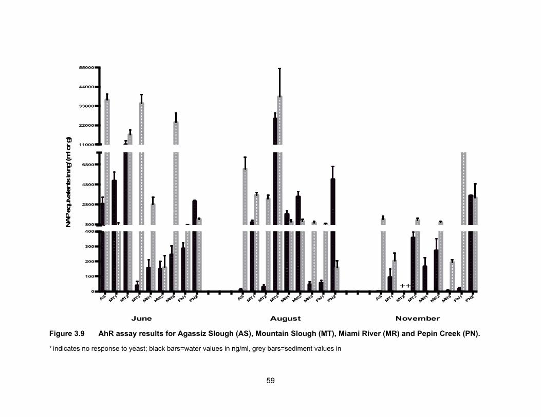
Urban developments such as a golf course (MR2), Harrison town centre (MR3)

and Aldergrove regional park (PN2) may contribute to AhR activity due to combustion,

leachate of construction material and oil/grease into waterways, and presence of high

traffic (Qin et al., 2014; Cailleaud et al., 2007; Jalova et al., 2013)

Overall, 75% of the sites from the same body of water had very similar levels of

AhR agonists’ contamination in the month of August. Our results are very close to ones

reported by Tam et al. (2001) from China where the AhR agonists were in the range of

356 to11098 ng/g.

58

Table 3.5 Summary of AhR agonists levels in water and sediments from Agassiz Slough, Mountain Slough, Miami River and Pepin Creek.

Sampling

Period

Sample

Type*

Agassiz Slough (AS)

L H M


L H M

Miami River (MR)

L H M

Pepin Creek (PN)

L H M

June

water 2105 3498 2851 10 12990 5423 98 301 184 245 3199 1710

sediment 33005 39578 36528 345 38789 17254 88 28780 8849 689 1396 1025

August

water 4 19 11 17 28008 8856 34 3999 1825 41 6808 2995

sediment 4976 7274 6349 3001 44789 15130 817 1345 1037 114 887 508

November

water BLD 45 398 226 4 335 148 6 3711 1843

sediment 915 1540 1311 155 1409 719 177 1123 594 2077 10459 6130

*Concentrations in water and sediment are presented in ng NAPEQs/ml and ng NAPEQs/g respectively. L=Low, H=High, M=Mean. Note the values are rounded to the nearest whole number for clarity.

59

Figure 3.9 AhR assay results for Agassiz Slough (AS), Mountain Slough (MT), Miami River (MR) and Pepin Creek (PN).

+ indicates no response to yeast; black bars=water values in ng/ml, grey bars=sediment values in

AS

MT1

MT2

MT3

MR1

MR2

MR3

PN1

PN2

AS

MT1

MT2

MT3

MR1

MR2

MR3

PN1

PN2

AS

MT1

MT2

MT3

MR1

MR2

MR3

PN1

PN2

0

100

200

300

400

800

2800

4800

6800

11000

22000

33000

44000

55000

June August November

NAP e

quiv

alents

in n

g/ (m

l or g)

++

60

Figure 3.10 Sites in 2013 sampling period with NAPEQs levels shown as dots. Sizes of dots are proportional to the amount of NAPEQs in water and sediments from all sampling periods.

61

3.4 EDCs levels from sampling sites in 2014/15

An area in Surrey was selected to test for EDCs since these sites are impacted by

anthropogenic activities while draining into a Nicomekl river, a fish-bearing watercourse.

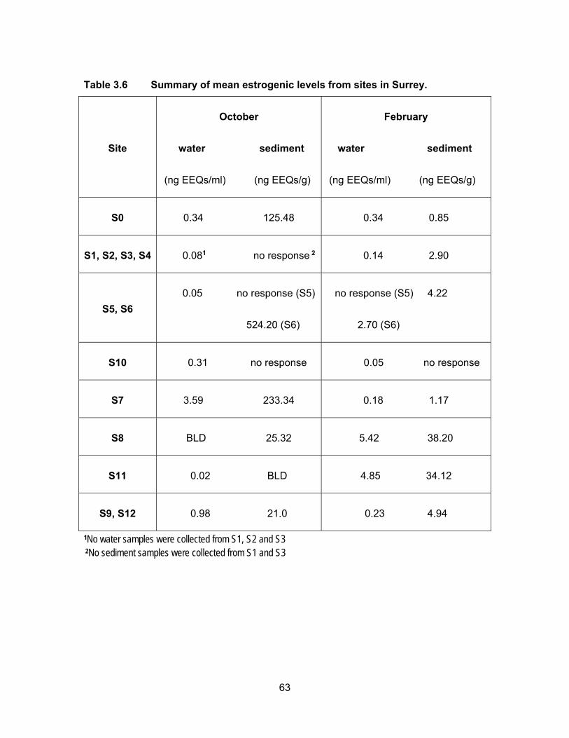
Table 2.2 summarizes each sampling site and a description of possible impacts on the

sites. S0 site is not connected to any other site; S1-S4 all catch water flows from the pump

station; S5 and S6 are impacted by berry farms as well as flows from the pump station;

S10 is downstream from a horse racetrack; S7 collects everything coming down from S1-

S6 and S10; S8 is downstream of all the sites mentioned above plus there may be some

influence from more dairy farmlands in between; S11 collects everything from the sites

mentioned above and it is also the last site before water enters Nicomekl river; S9 and

S12 are located in the Nicomekl river.

Since the ditches had very little or no water in October no results are presented

from site S2; and due to inaccessibility, no water and sediments were collected from sites

S1 and S3 in October.

3.4.1 Estrogenic levels in water and sediments

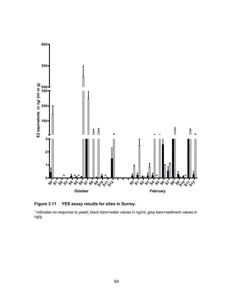
Results from the YES assay are presented in Table 3.6 and Figure 3.11 show the

results of YES bioassay on water and sediment samples, respectively in ng EEQs/ml and

ng EEQs/g. Figure 3.12 shows EEQs as dots of sizes that are proportional to amount of

estrogenic activity in water and sediments for both sampling periods.

3.4.1.1 Estrogenic levels in water

All water samples were responsive to the yeast cells in both sampling periods with

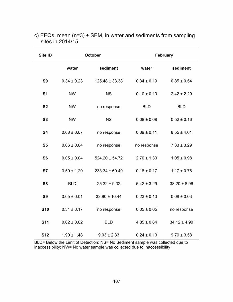
the exception of site S5 in February. Estrogenic activity was found to range from BLD to

3.97 ng EEQs/ml in October and from BLD to 6.02 ng EEQs/ml in February. In October

the mean EEQs were BLD, i.e., <0.0125 ng/ml for site S8 and very low (~ 0.04 ng EEQ/ml)

at sites S4, S5, S6, S9 and S11. The highest average concentrations were measured at

S7 (3.59 ng EEQs/ml) and S12 (1.90 ng EEQs/ml). In February, the estrogenicity in water

was very close to what had been measured in October’s samples. With higher water levels

in February, the estrogenicity for S1, S2 and S3 were very low; BLD for S2 and ~ 0.09 ng

62

EEQ/ml for S1 and S3. EEQs levels at S0 were the same for both sampling periods.

Compare to October, average EEQs levels in February were higher for S4, S6, S8, S9

and S11 and were lower at S7, S10 and S12. The highest activities were found in S8 (5.42

ng EEQ/ml) and S11 (4.85 ng EEQ/ml) in February. A possible explanation for the

variation in estrogenic activity near dairy farms is a change in rate of excretion during

pregnancy and lactation periods in cattle. In addition, an increase or decrease in the

number of animals during the time of sampling can influence the levels of EEQs detected

in the runoffs (Hanselman et al., 2003).

3.4.1.2 Estrogenic levels in sediments

Figure 3.11 shows the estrogenic levels for all sites in sediment samples. Unlike

water samples, there were 4 sites where sediments were non-responsive to the yeasts.

These sites included S2, S4, S5 and S10 in October and S10 in February. In October the

highest estrogenic levels were at S6 (524.20 ng EEQ/g) that had collected all the flow from

the pump station and berry farms, followed by site S7 (233.34 ng EEQ/g) which received

flow from pump station, berry farms and horse racetrack. S0 site also had high mean

estrogenic levels at 125.48 ng EEQ/g. The levels in Nicomekl River were 32.90 ng EEQ/g

and 9.03 ng EEQ/g for S9 (downstream) and S12 (upstream) respectively. Dilution could

be a factor in decrease levels down the river. Most of the sites had lower estrogenic levels

in sediments in February compared to in October. This could be due to more rainfall

causing dilution.

On average, the estrogenic contamination was much lower in water in both

seasons compare to levels in the sediments. Concentrations in sediments were either, on

average, higher or had no response in October compare to the sediment samples in

February. Higher levels in rainy period were expected as estrogens are degraded more

rapidly in warmer temperature. Less sunlight to cause abiotic degradation and lower rates

of microbial breakdown are other explanations for higher levels in sediment in October

(Tiryaki and Temur, 2010).

63

Table 3.6 Summary of mean estrogenic levels from sites in Surrey.

Site

October

water sediment

(ng EEQs/ml) (ng EEQs/g)

February

water sediment

(ng EEQs/ml) (ng EEQs/g)

S0 0.34 125.48 0.34 0.85

S1, S2, S3, S4 0.081 no response 2 0.14 2.90

S5, S6

0.05 no response (S5)

524.20 (S6)

no response (S5) 4.22

2.70 (S6)

S10 0.31 no response 0.05 no response

S7 3.59 233.34 0.18 1.17

S8 BLD 25.32 5.42 38.20

S11 0.02 BLD 4.85 34.12

S9, S12 0.98 21.0 0.23 4.94

1No water samples were collected from S1, S2 and S3 2No sediment samples were collected from S1 and S3

64

Figure 3.11 YES assay results for sites in Surrey.


S0 S1 S2 S3 S4 S5 S6 S7 S8 S9S10 S11 S12 S0 S1 S2 S3 S4 S5 S6 S7 S8 S9

S10 S11 S120

1

2

3

100

200

300500

550

600

E2

equ

ival

ents

in

ng

/ (m

l o

r g

)

October February

+ + + + + +

65

Figure 3.12 Sites in Surrey with EEQs levels shown as dots.

Sizes of dots are proportional to the amount of EEQs in water and sediments from all sampling periods.

3.4.2 Androgenic levels in water and sediments

Results from the YAS assay are presented in Table 3.7 and Figure 3.13; they are

expressed as ng of TbEQs per ml and g of water and sediments, respectively. Figure 3.14

shows TbEQs as dots of sizes that are proportional to amount of androgenic activity in

water and sediments for both sampling periods.

66

3.4.2.1 Androgenic levels in water

About 30% of the sites in October were BLD of 0.10 ng/ml of the YAS assay. In

addition, two sites were non responsive to yeast and the remaining sites had very low

TbEQs of approximately 1.18 ng TbEQ/ml. However, S8 and S9 stood out as having very

high levels at 150.58 ng TbEQs/ml and 115.05 ng TbEQs/ml respectively. The high levels

of androgenic activity at S8 possibly are due to runoff from the nearby dairy farms. There

is also a nursery and a horseback riding school close to these two locations. Cows were

also spotted in a close by field in October. Schiffer et al. (2001) found androgenic

compounds, Tb and MGA, in dairy farms runoffs and determined that the stability of Tb

can be up to 8 weeks after application on the field in manure. Only two sites had no

response to yeast in October (Table 3.7). In February, most sites had androgenic

contamination levels at around 0.60 ng TbEQs/ml. There was a decrease in TbEQs in the

S0, S8 and S9 sites in February compared to levels in October. Nevertheless S8 still had

the highest level out of all locations in February at 23.90 ng TbEQ/ml. Other locations

where androgenicity increased were S4 (23% up), S7 (33%), S10 (7%), S11 (3.5%) and

S12 (1.5%).

3.4.2.2 Androgenic levels in sediments

Androgenic contamination in sediments was higher than in water for both sampling

period (Figure 3.13). There was one sediment sample (S6) which was non responsive to

yeast from October sampling period. Androgenicity ranged from an average of 2.72 to

260.25 ng TbEQs/g were found in the sediments. The highest activity was found at S4.

This may be due to the application of fertilizer on the berry field from which runoffs get into

S4. In February the levels were lower compared to October sediment samples. There were

three samples (S1, S4, S8) found to be non responsive to yeast and one (S3) where levels

were BLD. The highest activity was at site S2 at 31.73 ng TbEQs/g; this site is the closest

point receiving flow from the pump station. The same site also had a high level of 84.37

ng TbEQs/g in October. According to Phillips et al. (2012) concentrations of androgens

are 10x higher in sewer output compared to discharge from a treated wastewater plant.

The site with the second highest activity was S9 at 27.78 ng TbEQ/g. The rest of the sites

were averaged at 4.56 ng TbEQ/g.

67

Table 3.7 Summary of mean androgenic levels from sites in Surrey.

Site October

water sediment

(ng TbEQs/ml) (ng TbEQs/g)

February

water sediment

(ng TbEQs/ml) (ng TbEQs/g)

S0 0.74 18.53 0.28 3.43

S1, S2, S3, S4 0.901 172.312

5.42 no response (S1, S4)

15.87

S5, S6

no response 16.09 (S5)

no response (S6)

0.20 8.12

S10 BLD 8.98 0.70 3.15

S7 BLD 43.21 3.31 0.50

S8 150.58 15.69 23.90 no response

S11 BLD 2.72 0.35 2.42

S9, S12 58.11 20.31 4.30 15.59


68

Figure 3.13 YAS assay results for sites in Surrey.


S0 S1 S2 S3 S4 S5 S6 S7 S8 S9S10S11S12 S0 S1 S2 S3 S4 S5 S6 S7 S8 S9

S10S11S120

15

30

100

200

280

320

October February

+ ++ + + +

Tb

eq

uiv

ale

nts

in n

g/ (

ml o

r g

)

69

Figure 3.14 Sites in Surrey with TbEQs levels shown as dots.

Sizes of dots are proportional to the amount of TbEQs in water and sediments from all sampling periods.

3.4.3 Glucocorticoid levels in water and sediments

Results from YGS assay are presented in Table 3.8 and Figure 3.15. The results

are expressed in ng of DOCEQs per ml and g of water and sediment sample, respectively.

Figure 3.16 shows DOCEQs as dots of sizes that are proportional to amount of

glucocorticoid activity in water and sediments for both sampling periods.

3.4.3.1 Glucocorticoid levels in water

Glucocorticoid levels in water ranged from BLD of 0.88 ng DOCEQs/ml at S11 to

22.28 ng DOCEQs/ml at S12 in October. Only S10 sample was non responsive to yeast.

The DOCEQs at Nikomekl River were highest upstream at S12 and dropped downstream

70

(S9) to 3.40 DOCEQs in ng/ml. Location S8, which is close to dairy farms, horse riding

school and an animal care facility, had the second highest levels of 18.59 ng DOCEQs/ml.

S0 site also had high levels at 17.21 ng DOCEQs/ml. The rest of the sites were on average

5.41 ng DOCEQs/ml. In February, only S12 sample was non responsive to yeast whereas

four samples were BLD from sites S0, S5, S7 and S11. This could be due to dilution factor

because of rainy period as these sites had higher water levels in October. The highest

level in February was detected in S2 (243.0 ng DOCEQs/ml), which receives effluent

directly from a pump station. Macikova et al. (2014) reported the highest glucocorticoid

receptor activity using GR-CALUX assay from an untreated wastewater (387.5 ng

DOCEQs/ml) compared to treated wastewater (35.0 ng DOCEQs/ml) and river water (1.9

ng DOCEQs/ml). My results are consistent with their findings in that the receiving end of

pump station had high levels compared to levels in the river and during rainy period.

3.4.3.2 Glucocorticoid levels in sediments

Table 3.8 shows that the sediments samples in October and February are similar.

For example, S0 site had no detectable glucocorticoid activity in both sampling period; S6,

S7 and S12 samples were non responsive to yeast in both time periods. Two more sites’

(S2 & S10) samples were also non responsive to yeast in October. The highest mean

activity was in S4 (776.50 ng DOCEQ/g), S5 (133.88 ng DOCEQ/g) and S8 (124.08 ng

DOCEQ/g). S4 receives untreated water from a liquid waste pump station that collects

sewer from storm drain. S5 gets water from S4 as well as runoff from a berry farm, and

S8 is influenced by dairy farms close by. In February, glucocorticoid activity was lower in

two sites but increased in two others. Thus, levels in S4 and S5 dropped to 55.20 ng

DOCEQs/g and 40.10 ng DOCEQs/g respectively. Glucocorticoid levels rose in S8 to

245.10 ng DOCEQs/g and in S9 to 57.70 ng DOCEQs/g in February. These two sites are

close to dairy farms, a horse riding school and also a dog and cat boarding site. The three

sites, S2, S3, S4, receiving water from the pump station had levels not significantly

different from each other at p < 0.05; all average at ~ 44.50 ng DOCEQs/g each site.

Sediments from site 10, which is influenced by a horse race track nearby, had levels at

24.26 ng DOCEQs/g very close to what was found in water (24.52 ng DOCEQs/ml)

71

High levels of glucocorticoid activity in sites close to land with cows, horses and

other small animals (animal care facility) suggest either use of anti-inflammatory drugs in

animals which are excreted in urine and feces (Mostle et al., 1999; Popot et al., 2006) or

social stress in animals which causes an increase in free cortisol in animal excreta

(Alexander & Irvine 1998) or use of fertilizers laden with antibiotics.

72

Table 3.8 Summary of mean glucocorticoid levels from sites in Surrey.

Site October

water sediment

(ng DOCEQs/ml) (ng DOCEQs/g)

February

water sediment

(ng DOCEQs/ml) (ng DOCEQs/g)

S0 17.21 BLD BLD BLD

S1, S2, S3, S4

6.021 no response (S2)

776.50 (S4)

63.05 47.29

S5, S6

9.98 133.88 (S5)

no response (S6)

7.04 40.10 (S5)

no response (S6)

S10 no response no response 24.52 24.26

S7 3.03 no response BLD no response

S8 18.59 124.08 143.53 245.10

S11 BLD 2.10 BLD 2.73

S9, S12

12.84 28.87 (S9)

no response (S12)

25.23 (S9) 57.70 (S9)

no response, no response (S12)

1No water samples were collected from S1, S2 and S3

73

1No water samples were collected from S1, S2 and S3

Figure 3.15 YGS Assay results for sites in Surrey.


S0 S1 S2 S3 S4 S5 S6 S7 S8 S9S10S11 S12 S0 S1 S2 S3 S4 S5 S6 S7 S8 S9

S10S11 S120

10

20

100

200

300

750

780

810

840

DO

C e

qu

iva

len

ts in

ng

/ (m

l or

g)

October February

+++ + + +++ ++

74

Figure 3.16 Sites in Surrey with DOCEQs levels shown as dots.

Sizes of dots are proportional to the amount of DOCEQs in water and sediments from all sampling periods.

3.4.4 Aryl Hydrocarbon receptor agonists levels in water and sediments

Results from AhR binding assay are presented in Table 3.9 and Figure 3.17. The

results are expressed in ng of β-Naphthoflavone equivalents (NAPEQs) per ml and g of

water and sediments, respectively. Figure 3.18 shows NAPEQs as dots of sizes that are

proportional to amount of AhR activity in water and sediments for both sampling periods.

75

3.4.4.1 AhR agonists levels in water

For water samples, 9 out of 10 tested positive for AhR activity in October and 11

out of 13 were positive in February. There was one S4 site that had no response to yeast

in October otherwise the NAPEQs ranged from 14.77 – 374.80 ng/ml. The three highest

levels of contamination were found at S10 (232.34 ng NAPEQs/ml), S11 (374.80 ng

NAPEQs/ml) and S12 (337.05 ng NAPEQs/ml). All three sites are close to roadways;

especially S10 and S12 are on the highway. This is due to vehicle emission and asphalt

contaminating the waterways (Qin et al., 2014). In February, AhR activity was the highest

at only one location, S8, at 626.10 ng NAPEQ/ml. This was much higher than what was

observed in October at being only 14.77 ng NAPEQs/ml. S8 is also on the street and

higher traffic in February is one explanation. This site is also influenced by nearby

farmlands that may have been using pesticides on the fields. The levels either dropped or

increased in February compared to results in October and that could be due to other

factors such as temperature, PAHs solubility, dilution or use of pesticides or contaminated

manure in the surrounding farmlands (Tremblay et al., 2005).

3.4.4.2 AhR agonists levels in sediments

Figure 3.17 shows that levels in sediments were higher than water. This was

expected since PAHs are more likely to adsorb onto organic matter than remain in the

water phase. None of the samples showed non-responsiveness to the yeasts in both

sampling periods (Table 3.9). The average NAPEQs ranged from 126.91 – 4489.21 ng/g

in October. The highest at the S12 location was near a busy highway. The NAPEQs for

S12 were not significantly different in February sitting at 4945.34 ng NAPEQs/g. In

February 85% of the sites had lower NAPEQs compared to values in October. This is

explained by higher ambient temperature in February that caused decrease in sorption of

PAHs to sediments (Hiller et al., 2008).

76

Table 3.9 Summary of mean AhR agonists’ levels from sites in Surrey.

Site October

water sediment

(ng NAPEQs/ml) (ng NAPEQs/g)

February

water sediment

(ng NAPEQs/ml) (ng NAPEQs/g)

S0 15.67 1574.39 3.71 335.00

S1, S2, S3, S4 no response1 2134.502 27.92 681.24

S5, S6 49.02 523.73 32.55 132.21

S10 232.34 1913.44 21.99 63.04

S7 32.26 332.82 85.10 7727.43

S8 14.77 176.63 626.10 436.89

S11 374.80 545.98 20.60 514.11

S9, S12 179.11 2308.06

75.40 (S9) 2524.5

no response (S12)


77

Figure 3.17 AhR Assay results for sites in Surrey.


S0 S1 S2 S3 S4 S5 S6 S7 S8 S9S10 S11 S12 S0 S1 S2 S3 S4 S5 S6 S7 S8 S9

S10 S11 S120

40

80

1000

2000

3000

6000

9000

NA

P e

qu

iva

len

ts i

n n

g/ (

ml o

r g

)

October February

+ +

78

Figure 3.18 Sites in Surrey with NAPEQs levels shown as dots.

Sizes of dots are proportional to the amount of NAPEQs in water and sediments from all sampling periods.

3.5 Results from Chemical Analyses

Chemical analysis using GC-MS was performed to identify compounds that were

contributing to EDC activity in the estrogenic, androgenic and AhR agonist bioassays.

The three water samples (AS, MR1, MR3) with high levels of estrogenic activity in

the YES assay were analyzed for estrogenic compounds using GC-MSD. The Total Ion

Current (TIC) chromatogram for the six standards is shown in Figure 3.19. The six

standard peaks, visible in the chromatogram, are of nonylphenol (NP), bisphenol A (BPA),

estrone (E1), 17β-estradiol (E2), 17β- ethynylestradiol (EE2) and estriol (E3). The

79

concentrations used were 1452.2 ng NP/ml, 1780.5 ng BPA/ml, 1614.1 ng E1/ml, 1875.6

ng E2/ml, 1599.0 ng EE2/ml and 1465.5 ng E3/ml. The calibration curves for each

standard are available in Appendix G. Results of the analyses showed the presence of

two steroidal chemicals, E2, E1 and one industrial EDC, BPA (Figure 3.20 & Appendix G).

The EEQs of each detectable compound were calculated using estradiol equivalency

factor (EEF) that were 1.0, 0.11 and 0.0004 for E2, E1 and BPA respectively (Vega-

Morales et al., 2013). The total EEQs obtained through chemical analysis was 11.6 ng

EEQs/ml whereas the total EEQs calculated from the yeast bioassay was 48.8 ng

EEQs/ml. The higher concentrations obtained from the yeast assay is likely because

recombinant yeast responds to any chemical that can activate the estrogen receptor

whereas only six estrogenic chemicals were targeted in the chemical analysis.

Two water samples (MT3 and MR3) with high androgenic activity in the YAS assay

were also selected for analysis using GC/MSD; in particular, to detect trenbolone as it is

often used as a growth promoter in dairy farms (Schiffer et al., 2001). Concentrations for

standards were 2389.4 ng DHT/ml and 1564.8 ng Tb/ml. TIC of the standard androgenic

compounds, dihydrotestosterone (DHT) and trenbolone (Tb), showed visible peaks for

each standard (Figure 3.21). However, no androgenic compounds were detected in the

water samples other than dehydroabietic acid (DHAA) (Appendix G). DHAA is a

component of resin acid found in coniferous trees and is detected in effluents of pulp and

paper mills. DHAA can be reduced by microorganisms to retene, a PAH, that can activate

the AhR receptor (Scott et al., 2011). Likewise, these samples also had activity in the AhR

assay. DHAA in the samples with positive results in the YAS bioassay suggests that DHAA

has androgenic activity since androgen receptor is activated. Other studies have reported

that DHAA may have endocrine disrupting properties. Masculinization of female

mosquitofish was observed in pulp mills effluents in the USA (Howell et al., 1980); female

guppies exposed to mill effluent developed secondary male sex characteristics (Larsson

et al., 2002) and in a study by Wartman et al. (2009), the androgenic potency to 3-spined

stickleback of pulp and paper mill effluent was found to be 4 times higher than the

estrogenic potency. Finally, an in vivo and in vitro study with goldfish and mosquitofish by

Ellis et al. (2003) have suggested androgenic activity in a pulp and paper mill effluent that

contained high amounts of DHAA.

80

No PAHs were detected through GC-MSD analysis possibly due to use of the full

scan mode rather than the selective ion monitoring mode (SIM) of analysis. Higher alkanes

such as tetra-, penta-, octadecanes; ei-, tri-, hexa-, octacosane; cyclohexane,

cyclotetracosane etc. were detected (see Appendix G). Possible sources of these

compounds are industrial lubricants, greases, diesel and aviation fuel (Sarker, M., 2011).

Although no chemical analysis was performed for samples from the city of Surrey,

a report by Metro Vancouver (2015) has confirmed presence of Brominated Diphenyl

Ethers (BDEs), Polyaromatic hydrocarbons (PAHs), Polychlorinated biphenyls (PCBs),

phenols and nonylphenols in the influent and effluent of the pump station. The pump

station (Figure 3.18) is located between S1 and S2. The detected PAHs that exceeded

the guideline values included pyrene, benzo(a)pyrene, anthracene and benzo (a)

anthracene. Detected PCBs included PCB 77, PCB 105, PCB 126 and PCB 169. Whereas

phenols as well as nonylphenol and ethoxylates had the highest levels compared to other

organic compounds of concern. Their report confirms our results from the AhR assay, as

the average NAPEQs were 14.50 – 71.13 ng/ml. The higher activity observed in the

bioassay is due to response of a mixture of chemicals including synergistic and

potentiation effects whereas data from Metro Vancouver (2013, 2015) is based on

individually detected compounds.

81

Figure 3.19 TIC of Estrogenic Standards: Nonylphenol (NP), Bisphenol A (BPA), Estrone (E1), 17β- Estradiol (E2), 17β- ethynylestradiol (EE2) and Estriol (E3).

82

Figure 3.20 TIC of E2, E1 and BPA detected in water samples

83

Figure 3.21 TIC of Androgenic Standards Dihydrotestosterone (DHT) and Trenbolone (Tb).

84

4. Risk to exposed species

Water and sediment quality objectives/guidelines for the protection of aquatic

species are based on exposure to single compounds. Thus, it is challenging to develop

guidelines based on the results of an effect-related yeast bioassay on chemical mixtures

that may interact with one another. However, concentrations obtained from the current

study can be compared to the levels set as guidelines for the purposes of risk assessment

if toxic equivalency factors (TEFs) are available for specific groups of EDCs.

Since there is no objective/guideline value available for NAPEQs, the

concentrations obtained through the yeast assay were converted into benzo [a] pyrene

equivalents (BAPEQs). Environment Canada has water and sediment quality guidelines

for the protection of aquatic life for some PAHs including benzo [a] pyrene (BAP). The

guideline for the protection of aquatic life is 0.015 ng/ml and 31.9 ng/g of BAP in water

and sediment, respectively (CCME, 1999). The concentrations measured in water and

sediment samples in the present study ranged from 0.34 - 7982.28 ng BAPEQ/ml and

3.71 - 12764.87 ng BAPEQ/g, for water and sediment, respectively. Thus levels in the

current study exceed the guideline values from Canadian Council of Ministers of the

Environment (CCME).

There are no objective/guideline for estradiol, androgens or glucocorticoid

equivalents for the protection of aquatic life under Canadian or British Columbia

water/sediment quality guidelines. A predicted no effect E2 concentration for the protection

of aquatic life derived by the European union is of 0.0004 ng/ml (SCHER, 2011) whereas

concentrations higher than 0.001 ng EEQ/ml are associated with adverse effects (UK

Environmental Agency, 2004). Other predicted no effect concentrations (PNECs) and

hazard concentrations based on no observed adverse effect levels (NOAEL) range from

0.00073 to 0.002 ng/ml of E2 (Wu et al., 2014). E2 values from the current study were

0.0125 – 29.3 ng EEQs/ml and therefore potentially may cause adverse effects on the

aquatic life in these sites.

As for the androgenic compounds, the reported toxicity in literature varies

depending on the type of androgens, sex of the fish, species tested and the endpoint

85

measured. One study found no effect of trenbolone at 0.02 ng/ml in courtship behavior of

zebrafish (Larsen & Baatrup, 2010) but 0.009 ng/ml of the same compound induced

irreversible masculinization in female zebrafish (Morthorst et al., 2010). Other studies have

reported LOAELs at 0.03 ng TbEQs/ml can reduce fecundity and at 0.4 ng TbEQs/ml can

affect secondary sex characteristics in different species of female fish (Ankley et al., 2003;

Seki et al., 2006). The range of TbEQs in the current study is 0.1 – 1577.30 ng/ml, higher

than the reported LOAELs and NOAELs in the literature. A proper risk assessment with

weight of evidence (WoE) approach is required to establish risk to the species inhabiting

the study areas.

Studies reporting the effects of synthetic glucocorticoids are rare. The study by

Kugathas and Sumpter (2011) reported that synthetic glucocorticoid concentration of 0.1

ng/ml (NOAEC) did not have statistically significant effects in aquatic organisms although

the LOAEC was found to be 1 ng/ml. Other studies have reported lethal effects on

reproduction, growth and development of fish exposed to 500 ng/ml of synthetic

glucocorticoids (LaLone et al., 2012). Glucocorticoid levels derived from the YGS bioassay

in the water and sediment samples from the current study were the highest among the

three steroid hormones; levels ranging from 0.75 – 8999.32 ng DOCEQs/ml in water and

0.75 – 18988.10 ng DOCEQs ng/g in sediments were found. These high concentrations

in the current study may cause adverse effects such as high plasma glucose

concentrations and compromised immune system in fish leading to susceptibility to

disease and other contaminants in the environment (Kugathas & Sumpter, 2011).

EDCs can alter a living organism in many ways depending on numerous factors.

Thus it is unreasonable to characterize a risk or no risk to the species living in these

waterways. In addition, as dose response is not always a monotonic relationship and high

concentrations have not been studied, it is uncertain if the high levels obtained in current

study reflect real exposure to these compounds because of the indirect nature of

bioassays. Overall one has to look at exposure levels, hazard, species susceptibility, life

stage and potency of the chemical mixture, to name a few, for a proper risk assessment

of the EDCs (Testai et al., 2013). In addition, other factors like pH, salinity, dissolved

oxygen concentration and presence of metals in the environment should also be taken

into consideration.

86

5. Study Limitations and Future Directions

Yeast bioassays are fast, cost effective and reliable way of testing for EDCs in the

environment. As there is an increase in environmental contamination and pollution with

rapid industrialization, these bioassays can provide a rapid screen for potential exposure

of wildlife to EDCs. Nevertheless these results do not directly predict the biological

response an animal would have to these compounds as we are dealing with mixtures of

EDCs and the pharmacokinetics (absorption, distribution, metabolism and elimination) of

these chemicals in aquatic species and wildlife are still not known.

Some suggested research studies in the future may include the following: (a)

improvement on the extraction methods to better recover EDCs from the samples (b)

spatial and temporal variation of EDC levels should be examined closely with regards to

the sources in order to protect the aquatic species in these areas; this can be achieved by

increasing sampling, examining reproducibility and validating results with chemical

analyses (c) more information such as habitat preference, foraging behaviour and other

characteristics on the species living in these sloughs, creeks, lake and river will enable a

site specific risk assessment of exposure.

87

References

Alexander, S. L., & Irvine, C. H. G. (1998). The effect of social stress on adrenal axis activity in horses: The importance of monitoring corticosteroid-binding globulin capacity. Journal of Endocrinology, 157(3), 425–432.

Alnafisi, A., Hughes, J., Wang, G., Miller, C. (2007). Evaluating polycyclic aromatic hydrocarbons using a yeast bioassay. Environmental Toxicology and Chemistry, 26(7), 1333-1339.

Ankley, G. T., Jensen, K. M., Makynen, E., Kahl, M. D., Korte, J. J., Hornung, M. W., Gray, L. E. (2003). Effects of the androgenic growth promoter 17-beta-trenbolone on fecundity and reproductive endocrinology of the fathead minnow. Environmental Toxicology and Chemistry / SETAC, 22(6), 1350–1360.

Antunes-Fernandes, E., Bovee, T., Daamen, F, Helsdingen, R., van den Berg, M., van Duursen, M. (2011). Some OH-PCBs are more potent inhibitors of aromatase activity and (anti-) glucocorticoids than non-dioxin like (NDL)-PCBs and MeSO2-PCBs. Toxicology Letters, 206, 158-165.

Atwater, J. W., Whalen, T. F., Dasika, R. (1998). Mushroom Waste Management Project. Liquid Waste Management-Phase I & Phase II. Environment Canada.

Balsiger, H. and Cox, M. (2009). Yeast-Based reporter assays for the functional characterization of cochaperone interactions with steroid hormone receptors. The Nuclear Receptor Superfamily, 505, 141-156.

Balsiger, H., de la Torre, R., Lee, W.Y., Cox, M. B. (2010). A Four-Hour Yeast Assay for the Direct Measure of Estrogenic Activity in Wastewater Without Sample Extraction, Concentration, or Sterilization. Science of the Total Environment, 408(6), 1422–1429.

Bazin I., Hassine A., Mnif W., Gonzalez, C. (2013). YES as a Tool for Detecting Estrogenic Activity of Some Food Additives Compounds: E 104, E 122, E 124, E 132 and E 171. Journal of Ecosystem & Ecography, 3(3), 128.

Bauer, E. R., Daxenberger, A, Petri, T., Sauerwein, H., Meyer, H. H. (2000). Characterisation of the affinity of different anabolics and synthetic hormones to the human androgen receptor, human sex hormone binding globulin and to the bovine progestin receptor. Apmis, 108(12), 838–846.

Bergman, Å., Heindel, J., Jobling, S., Kidd, K., Zoeller, R. T. (2012). State of the science of endocrine disrupting chemicals, 2012. United Nations Environment Programme and World Health Organization. (Vol. 211).

88

Bhattacharjee, G. & Khurana, S. (2014). In vitro Reporter Assays for Screening of Chemicals that disrupt Androgen Signaling. Journal of Toxicology, 1-7.

Bistan, M., Logar, R., Tišler, T. (2011). Detection of estrogenic activity in Slovenian wastewaters by bioassay. Open Life Sciences, 6(5), 829–837.

Bogdal, C., Naef, M., Schmid, P., Kohler, M., Zennegg, M., Bernet, D., Hungerbühler, K. (2009). Unexplained gonad alterations in whitefish (Coregonus spp.) from Lake Thun, Switzerland: Levels of persistent organic pollutants in different morphs. Chemosphere, 74(3), 434–440.

Boström, C.E., Gerde, P., Hanberg, A., Jernström, B., Johansson, C., Kyrklund, T., Westerholm, R. (2002). Cancer risk assessment, indicators, and guidelines for polycyclic aromatic hydrocarbons in the ambient air. Environmental Health Perspectives, 110, 451–488.

Bovee, T., Bor, G., Heskamp, H., Lasaroms, J., Sanders, M., Nielen, M. (2009). Validation and application of a yeast bioassay for screening androgenic activity in calf urine and feed. Analytica Chimica ACTA, 673, 225-234.

Bovee, T., Helsdingen, R., Hamer, A., Brouwer, B., Nielen, M. (2011). Recombinant cell bioassays for the detection of (gluco) corticosteroids and endocrine-disrupting potencies of several environmental PPCB contaminants. Anal Bioanal Chem, 401, 873-882.

Cailleaud, K., Forget-Leray, J., Souissi, S., Hilde, D., LeMenach, K., Budzinski, H. (2007). Seasonal variations of hydrophobic organic contaminant concentrations in the water-column of the Seine Estuary and their transfer to a planktonic species Eurytemora affinis (Calanoïda, copepoda). Part 1: PCBs and PAHs. Chemosphere, 70(2), 270–280.

Campbell, R. K., Satoh, N., Degnan, B. M. (2004). Piecing together evolution of the vertebrate endocrine system. Trends in Genetics, 20(8), 359–366.

Campbell, C., Borglin, S., Green, F., Grayson, A., Wozei, E., Stringfellow, W. (2006). Biologically directed environmental monitoring, fate, and transport of estrogenic endocrine disrupting compounds in water: A review. Chemosphere, 65, 1265-1280.

Canadian Council of Ministers of the Environment. (CCME 1999a). Canadian Sediment Quality Guidelines for the Protection of Aquatic Life - Polycyclic Aromatic Hydrocarbons. Canadian Environmental Quality Guidelines 1–16.

Canadian Council of Ministers of the Environment. (CCME 1999b). Canadian water quality guidelines for the protection of aquatic life - Polycylic aromatic hydrocarbons. Canadian Environmental Quality Guidelines, 1–13.

89

Chang, H., Choo, K., Lee, B., Choi, S. (2009). The methods of identification, analysis, and removal of endocrine disrupting compounds (EDCs) in water. Journal of Hazardous Materials, 172, 1-12.

Cheek, A. O., Vonier, P. M., Oberdörster, E., Burow, B. C., McLachlan, J. (1998). Environmental signaling: A biological context for endocrine disruption. Environmental Health Perspectives, 106(1), 5–10.

Cherlet, M., De Baere, S., De Backer, P. (2004). Quantitative determination of dexamethasone in bovine milk by liquid chromatography-atmospheric pressure chemical ionization-tandem mass spectrometry. Journal of Chromatography. B, Analytical Technologies in the Biomedical and Life Sciences, 805(1), 57–65.

Courtheyn, D., Vercammen, J., De Brabander, H. F., Vandenreyt, I., Batjoens, P., Vanoosthuyze, K., Van Peteghem, C. (1994). Determination of dexamethasone in urine and faeces of treated cattle with negative chemical ionization-mass spectrometry. The Analyst, 119(12), 2557–64.

Cox, M. and Miller, C. (2002). The p23 co-chaperone facilitates dioxin receptor signalling in a yeast model system. Toxicology Letters, 129, 13-21.

Damstra, T., Barlow, S., Bergman, A., Kavlock, R., Kraak, G. Van Der. (2002). International Programme on Chemical Safety. Global Assessment of the State of the Science of Endocrine Disruptors. World Health Organization.

De Clercq, N., Bussche, J. Vanden, Croubels, S., Delahaut, P., Vanhaecke, L. (2014). Development and validation of a high resolution mass spectrometry based method to study the long-term stability of natural and synthetic glucocorticoids in faeces. Journal of Chromatography A, 1336, 76–86.

Denison, M. S., Pandini, A, Nagy, S. R., Baldwin, E. P., Bonati, L. (2002). Ligand binding and activation of the Ah receptor. Chem Biol.Interact., 141, 3–24.

Durhan, E. J., Lambright, C. S., Makynen, E., Lazorchak, J., Hartig, P. C., Wilson, V. S., Ankley, G. T. (2006). Identification of metabolites of trenbolone acetate in androgenic runoff from a beef feedlot. Environmental Health Perspectives, 114(April), 65–68.

Eldridge, M. L., Sanseverino, J., Layton, C., Easter, J. P., Schultz, T. W., Sayler, G. S. (2007). Saccharomyces cerevisiae BLYAS, a New Bioluminescent Bioreporter for Detection of Androgenic Compounds. Applied and Environmental Microbiology, 73(19), 6012–6018.

Ellis, R. J., van den Heuvel, M. R., Bandelj, E., Smith, M., McCarthy, L. H., Stuthridge, T. R., Dietrich, D. R. (2003). In vivo and in vitro assessment of the androgenic potential of a pulp and paper mill effluent. Environmental Toxicology and Chemistry / SETAC, 22(7), 1448–1456.

90

Fent, K., Weston, A, Caminada, D. (2006). Ecotoxicology of human pharmaceuticals. Aquatic Toxicology, 76(2), 122–159.

Finlay-Moore, O., Hartel, P. G., Cabrera, M. L. (2000). 17β-estradiol and Testosterone in Soil and Runoff from Grasslands Amended with Broiler Litter. Journal of Environmental Quality, 29, 1604-1611.

Fisheries and Oceans Canada. (2010). Recovery strategy for the Salish Sucker (Catostomus sp.) in Canada. Species at Risk Act Recovery Strategy Series, Vancouver, vii +64

Gaido, K., Leonard, L., Lovell, S., Gould, J., Babai, D., Portier, C., McDonnell, D. (1997). Evaluation of Chemicals with Endocrine Modulating Activity in a Yeast-Based Steroid Hormone Receptor Gene Transcription Assay. Toxicology and Applied Pharmacology, 143, 205-212.

Giesy, J., Hilscherova, K., Jones, P., Kannan, K., Machala, M. (2002). Cell bioassays for detection of aryl hydrocarbon (AhR) and estrogen (ER) mediated activity in environmental samples. Marine Pollution Bulletin, 45, 3-16.

Hall, K. J., & Schreier, H. (1996). Urbanization and agricultural intensification in the Lower Fraser River valley : Impacts on water use and quality. GeoJournal, 40, 135–146.

Hanselman, T., Graetz, D., Wilkie, A. C. (2003). Manure-Borne Estrogens as Potential Environmental Contaminants: A Review. Environmental Science and Technology, 37(24), 5471–5478.

Hayes, T. B. (2005). Welcome to the revolution: integrative biology and assessing the impact of endocrine disruptors on environmental and public health. Integrative and Comparative Biology, 45(2), 321–329.

Hiller, E., Jurkovič, Ľ., Bartaľ, M. (2008). Effect of Temperature on the Distribution of Polycyclic Aromatic Hydrocarbons in Soil and Sediment, 2008(1), 231–240.

Hiller-Sturmhöfel, S., & Bartke, A. (1998). The Endocrine System: An overview. Alcohol Health and Research Worlds, 22(3), 153-164.

Howell, W. M., Black, D. A., Bortone, S. A. (1980). Abnormal Expression of Secondary Sex Characters in a Population of Mosquitofish, Gambusia affinis holbrooki: Evidence for Environmentally-induced Masculinization. COPEIA, 4, 676-681.

Huang, C. H., & Sedlak, D. L. (2001). Analysis of estrogenic hormones in municipal wastewater effluent and surface water using enzyme-linked immunosorbent assay and gas chromatography/tandem mass spectrometry. Environmental Toxicology and Chemistry / SETAC, 20(1), 133–139.

91

Huetos, O., Ramos, M., Martín de Pozuelo, M., San Andrés, M., Reuvers, T. B. (1999). Determination of dexamethasone in feed by TLC and HPLC. The Analyst, 124(11), 1583–7.

Iglesias, A., Nebot, C., Vázquez, B. I., Miranda, J. M., Abuín, C. M. F., Cepeda, A. (2014). Detection of veterinary drug residues in surface waters collected nearby farming areas in Galicia, North of Spain. Environmental Science and Pollution Research, 21(3), 2367–2377.

Ishibashi, H., Tachibana, K., Tsuchimoto, M., Soyano, K., Ishibashi, Y., Nagae, M., Arizono, K. (2001). In vivo testing system for determining the estrogenic activity of endocrine-disrupting chemicals (EDCs) in goldfish (Carassius auratus). Journal of Health Science, 47(2), 213–218.

Jálová, V., Jarošová, B., Bláha, L., Giesy, J. P., Ocelka, T., Grabic, R., Hilscherová, K. (2013). Estrogen-, androgen- and aryl hydrocarbon receptor mediated activities in passive and composite samples from municipal waste and surface waters. Environment International, 59, 372–383.

Jobling, S., Casey, D., Rodgers-Gray, T., Oehlmann, J., Schulte-Oehlmann, U., Pawlowski, S., Tyler, C. (2003). Comparative responses of molluscs and fish to environmental estrogens and an estrogenic effluent. Aquatic Toxicology, 65(2), 205–220.

Jobling, S., Sheahan, D., Osborne, J., Matthiessen, P., Sumpter, J. P. (1996). Inhibition of testicular growth in rainbow trout (Oncorhynchus mykiss) exposed to estrogenic alkylphenolic chemicals. Environmental Toxicology and Chemistry, 15(2), 194–202.

Kato, Y., Ikushiro, S., Haraguchi, K., Yamazaki, T., Ito, Y., Suzuki, H., Kimura, R., Yamada, S., Inoue, T., Degawa, M. (2004). A Possible Mechanism for Decrease in Serum Thyroxine Level by Polychlorinated Biphenyls in Wistar and Gunn Rats. Toxicological Sciences, 81, 309-315.

Kidd, K., Blanchfield, P. J., Mills, K. H., Palace, V. P., Evans, R. E., Lazorchak, J. M., Flick, R. W. (2007). Collapse of a fish population after exposure to a synthetic estrogen. Proceedings of the National Academy of Sciences of the United States of America, 104(21), 8897–8901.

Kinnberg, K., Korsgaard, B., Bjerregaard, P., Jespersen, A. (2000). Effects of nonylphenol and 17beta-estradiol on vitellogenin synthesis and testis morphology in male platyfish Xiphophorus maculatus. The Journal of Experimental Biology, 203, 171–81.

Knudsen, F. R., & Pottinger, T. G. (1999). Interaction of endocrine disrupting chemicals, singly and in combination, with estrogen-, androgen-, and corticosteroid-binding sites in rainbow trout (Oncorhynchus mykiss). Aquatic Toxicology, 44(3), 159–170.

92

Kojima, H., Takeuchi, S., Nagai, T. (2010). Endocrine-disrupting Potential of Pesticides via Nuclear Receptors and Aryl Hydrocarbon Receptor. Journal of Health Science, 56(4), 374–386.

Kolok, A. S., & Sellin, M. K. (2008). The environmental impact of growth-promoting compounds employed by the United States beef cattle industry: history, current knowledge, and future directions. Reviews of Environmental Contamination and Toxicology, 195, 1–30.

Krishnan, A.V., Stathis, P., Permuth, S.F., Tokes, L., Feldman, D. (1993). Bisphenol-A: Estrogenic substance is released from polycarbonate flasks during autoclaving. Endocrinology, 132(6), 2279–2286.

Kugathas, S. & Sumpter, J. (2011). Synthetic glucocorticoids in the Environment: First Results on Their Potential Impacts on Fish. Environmental Science & Technology, 45, 2377–2383.

Kurosawa, T., Hiroi, H., Tsutsumi, O., Ishikawa, T., Osuga, Y., Fujiwara, T., Taketani, Y. (2002). The activity of bisphenol A depends on both the estrogen receptor subtype and the cell type. Endocrine Journal, 49(4), 465-471.

LaLone, C., Villeneuve, D. L., Olmstead, W., Medlock, E. K., Kahl, M. D., Jensen, K. M., Ankleyy, G. T. (2012). Effects of a glucocorticoid receptor agonist, dexamethasone, on fathead minnow reproduction, growth, and development. Environmental Toxicology and Chemistry, 31(3), 611–622.

Lange, I. G., Daxenberger, A., Schiffer, B., Witters, H., Ibarreta, D., Meyer, H. H. D. (2002). Sex hormones originating from different livestock production systems: Fate and potential disrupting activity in the environment. Analytica Chimica Acta, 473, 27–37.

Larsen, M. G., & Baatrup, E. (2010). Functional behavior and reproduction in androgenic sex reversed zebrafish (Danio rerio). Environmental Toxicology and Chemistry, 29(8), 1828–1833.

Larsson, D. G. J., Kinnberg, K., Sturve, J., Stephensen, E., Skön, M., Förlin, L. (2002). Studies of masculinization, detoxification, and oxidative stress responses in guppies (Poecilia reticulata) exposed to effluent from a pulp mill. Ecotoxicology and Environmental Safety, 52(1), 13–20.

Lintelmann, J., Katayama, A., Kurihara, N., Shore, L., Wenzel, A. (2003). Endocrine disruptors in the environment (IUPAC Technical Report ). Pure Appl. Chem., 75(5), 631–681.

Lorenzen, A., Hendel, J. G., Conn, K. L., Bittman, S., Kwabiah, A. B., Lazarovitz, G., Topp, E. (2004). Survey of hormone activities in municipal biosolids and animal manures. Environmental Toxicology, 19(3), 216–225.

93

Macikova, P., Groh, K. J., Ammann, A., Schirmer, K., Suter, M. J.-F. (2014). Endocrine disrupting compounds affecting corticosteroid signaling pathways in Czech and Swiss waters: potential impact on fish. Environmental Science & Technology, 48(21), 12902–11.

Martinez, E., Gros, M., Lacorte, S., Barceló, D. (2004). Simplified procedures for the analysis of polycyclic aromatic hydrocarbons in water, sediments and mussels. Journal of Chromatography A, 1047(2), 181–188.

Matthews, A. & Gustafsson, J. (2006). Estrogen receptor and aryl hydrocarbon receptor signaling pathways. Nuclear Receptor Signaling, 4, e016.

Matthews, J. B., Twomey, K., Zacharewski, T. R. (2001). In Vitro and in Vivo Interactions of Bisphenol A and Its Metabolite, Bisphenol A Glucuronide, with Estrogen Receptors α and β. Chemical Research in Toxicology, 14(2), 149-157.

Metro Vancouver (2013). Sanitary sewer overflow risk assessment of interim management options: Lynn branch siphon, Katzie pump station and Cloverdale pump station. Report by Tetra Tech, Vancouver, B.C., Canada.

Metro Vancouver (2015). Update of Screening level human health and ecological risk assessment for sanitary sewer overflows: Cloverdale pump station, Lynn Branch siphon and Katzie pump station. Report prepared by SLR global environmental solutions, Vancouver, B.C., Canada.

Miksicek, R. J. (1995). Estrogenic Flavonoids: Structural Requirements For Biological Activity. Proc. Soc. Exp. Biol. Med, (208), 44–50.

Ministry of Environment, British Columbia (BC). (2002). Wildlife in British Columbia at Risk: Oregon Spotted Frog. http://www.gov.bc.ca/.

Morthorst, J. E., Holbech, H., Bjerregaard, P. (2010). Trenbolone causes irreversible masculinization of zebrafish at environmentally relevant concentrations. Aquatic Toxicology, 98(4), 336–343.

Möstl, E., Messmann, S., Bagu, E., Robia, C., Palme, R. (1999). Measurement of glucocorticoid metabolite concentrations in faeces of domestic livestock. Journal of Veterinary Medicine A, 46(10), 621–631.

Nichols, D. J., Daniel, T. C., Moore, P., Edwards, D. R., Pote, D. H. (1997). Runoff of Estrogen Hormone 17β-Estradiol from Poultry Litter Applied to Pasture. Journal of Environment Quality, 26(4), 1002.

Nie, Y., Qiang, Z., Zhang, H., Adams, C. (2009). Determination of endocrine-disrupting chemicals in the liquid and solid phases of activated sludge by solid phase extraction and gas chromatography-mass spectrometry. Journal of Chromatography. A, 1216(42), 7071–80.

94

Noguerol, T. N., Boronat, S., Casado, M., Raldúa, D., Barceló, D., Piña, B. (2006). Evaluating the interactions of vertebrate receptors with persistent pollutants and antifouling pesticides using recombinant yeast assays. Analytical and Bioanalytical Chemistry, 385(6), 1012–1019.

Norris, D. & Lopez, K (2011). Hormones and Reproduction of Vertebrates. Fishes, Volume 1. Academic Press. San Diego, CA.

Palace, V., Evans, R., Wautier, K., Mills, K., Blanchfield, P., Park, B., Kidd, K. (2009). Interspecies differences in biochemical, histopathological, and population responses in four wild fish species exposed to ethynylestradiol added to a whole lake. Canadian Journal of Fisheries and Aquatic Sciences, 66(11), 1920–1935.

Parker, J., Webster, J. P., Kover, S. C., Kolodziej, E. P. (2012). Analysis of trenbolone acetate metabolites and melengestrol in environmental matrices using gas chromatography-tandem mass spectrometry. Talanta, 99, 238–46.

Patel, M. R., Scheffler, B. E., Wang, L., Willett, K. L. (2006). Effects of benzo(a)pyrene exposure on killifish (Fundulus heteroclitus) aromatase activities and mRNA. Aquatic Toxicology (Amsterdam, Netherlands), 77(3), 267–78.

Peck, M., Gibson, R. W., Kortenkamp, A., Hill, E. M. (2004). Sediments are major sinks of steroidal estrogens in two United Kingdom rivers. Environmental Toxicology and Chemistry / SETAC, 23(4), 945–952.

Phillips, P. J., Chalmers, T., Gray, J. L., Kolpin, D. W., Foreman, W. T., Wall, G. R. (2012). Combined sewer overflows: An environmental source of hormones and wastewater micropollutants. Environmental Science & Technology, 46, 5336–5343.

Pocar, P., Fischer, B., Klonisch, T., Hombach-Klonisch, S. (2005). Molecular interactions of the aryl hydrocarbon receptor and its biological and toxicological relevance for reproduction. Reproduction, 129, 379–389.

Popot, M., Donval, A, Bonnaire, Y., Huau, J. (2006). Use of accelerating solvent extraction for detecting non-steroidal anti-inflammatory drugs in horse feces. Journal of Analytical Toxicology, 30(5), 323–30.

Qin, N., He, W., Kong, X.-Z., Liu, W.-X., He, Q.-S., Yang, B., Zhao, X.-L. (2014). Distribution, partitioning and sources of polycyclic aromatic hydrocarbons in the water-SPM-sediment system of Lake Chaohu, China. The Science of the Total Environment, 496, 414–23.

Reig, M., Mora, L., Flores, M., Toldrá, F. (2006). HPLC Method for the Analysis of Dexamethasone in feed and water for Livestock. 52nd International Congress of Meat Science and Technology: Harnessing and Exploiting Global Opportunities. Wageningen. Academic Publishers. Netherlands. 365-366.

95

Riggs, D. L., Roberts, P. J., Chirillo, S. C., Cheung-Flynn, J., Prapapanich, V., Ratajczak, T., Smith, D. F. (2003). The Hsp90-binding peptidylprolyl isomerase FKBP52 potentiates glucocorticoid signaling in vivo. The European Molecular Biology Organization Journal, 22(5), 1158–67.

Rosen, M. R., Goodbred, S. L., Patiño, R., Leiker, T. J., Orsak, E. (2007). Investigations of the Effects of Synthetic Chemicals on the Endocrine System of Common Carp in Lake Mead, Nevada and Arizona. Publications of the US Geological Survey. Paper 80.

Sanseverino, J., Gupta, R. K., Layton, A., Patterson, S. S., Ripp, S., Saidak, L., Simpson, M. L., Schultz, T., Sayler, G. S. (2005). Use of. Saccharomyces cerevisiae BLYES Expressing Bacterial Bioluminescence for Rapid, Sensitive Detection of Estrogenic Compounds. Applied and Environmental Microbiology, 71(8), 4455–4460.

Sarker, M. (2007). Municipal Waste Plastic Conversion into Different Category of Liquid Hydrocarbon Fuel. Chemistry, Emission Control, Radioactive Pollution and Indoor Air Quality. InTech. 45-80.

SCHER (Scientific Committee on Health and Environmental Risks). (2011). Opinion on draft environmental quality standards under the Water Framework Directive – 17β-estradiol (E2), European Union (30 March).

Schiffer, B., Daxenberger, A., Meyer, K., Meyer, H. H. D. (2001). The fate of trenbolone acetate and melengestrol acetate after application as growth promoters in cattle: Environmental studies. Environmental Health Perspectives, 109(11), 1145–1151.

Scott, J., Incardona, J. P., Pelkki, K., Shepardson, S., Hodson, P. V. (2011). AhR2-mediated, CYP1A-independent cardiovascular toxicity in zebrafish (Danio rerio) embryos exposed to retene. Aquatic Toxicology, 101(1), 165–174.

Seki, M., Fujishima, S., Nozaka, T., Maeda, M., Kobayashi, K. (2006). Comparison of response to 17 beta-estradiol and 17 beta-trenbolone among three small fish species. Environmental Toxicology and Chemistry / SETAC, 25(10), 2742–2752.

Sellin, M. K., Snow, D. D., Gustafson, S. T., Erickson, G. E., Kolok, S. (2009). The endocrine activity of beef cattle wastes: do growth-promoting steroids make a difference? Aquat Toxicol, 92(4), 221–227.

Shi, J., Liu, X., Cao, J., Bo, T., Li, Y. (2013). Occurrence and Risk Assessment of Estrogens and Anti-Inflammatories in Baiyangdian Lake, North China. Environmental Engineering and Management Journal, 12(7), 1437–1445.

Shi, Z., Valdez, K. E., Ting, A. Y., Franczak, A., Gum, S. L., Petroff, B. K. (2007). Ovarian endocrine disruption underlies premature reproductive senescence following environmentally relevant chronic exposure to the aryl hydrocarbon receptor agonist 2,3,7,8-tetrachlorodibenzo-p-dioxin. Biology of Reproduction, 76(2), 198–202.

96

Shutt, D.A. (1976). The effects of plant oestrogens on animal reproduction. Endeavor, 35, 110-113.

Soto, A. M., Calabro, J. M., Prechtl, N. V., Yau, A. Y., Orlando, E. F., Daxenberger, A., Sonnenschein, C. (2004). Androgenic and Estrogenic Activity in Water Bodies Receiving Cattle Feedlot Effluent in Eastern Nebraska, USA. Environmental Health Perspectives, 112(3), 346–352.

Tabata, A., Kashiwada, S., Ohnishi, Y., Ishikawa, H., Miyamoto, N., Itoh, M., Magara, Y. (2001). Estrogenic influences of estradiol-17β, p-nonylphenol and bis-phenol-A on Japaneses Medaka (Oryzias latipes) at detected environmental concentrations. Water Science and Technology, 43(2), 109-116.

Takeda, T., Matsumoto, Y., Koga, T., Mutoh, J., Nishimura, Y., Shimazoe, T., Ishii, Y., Ishida, T., Yamada, H. (2009). Maternal exposure to Dioxin disrupts gonadotropin production in fetal rats and imprints defects in sexual behavior. The Journal of Pharmacology and Experimental Therapeutics, 329, 1091-1099.

Tam, N. F. Y., Ke, L., Wang, X. H., Wong, Y. S. (2001). Contamination of polycyclic aromatic hydrocarbons in surface sediments of mangrove swamps. Environmental Pollution, 114(2), 255–263.

Ternes, T., Andersen, H., Gilberg, D., Bonerz, M. (2002). Determination of estrogens in sludge and sediments by liquid extraction and GC/MS/MS. Analytical Chemistry, 74(14), 3498–3504.

Testai, E., Galli, C. L., Dekant, W., Marinovich, M., Piersma, A. H., Sharpe, R. M. (2013). A plea for risk assessment of endocrine disrupting chemicals. Toxicology, 314(1), 51–59.

Thorpe, K. L., Cummings, R. I., Hutchinson, T. H., Scholze, M., Brighty, G., Sumpter, J. P., Tyler, C. R. (2003). Relative Potencies and Combination Effects of Steroidal Estrogens in Fish. Environmental Science & Technology, 37(6), 1142–9.

Tierney, K., Farrell, A., Brauner, C. (2014). Organic Chemical Toxicology of Fishes. Fish Physiology, Volume 33. Academic Press. San Diego, CA.

Tilton, S. C., Foran, C. M., Benson, W. H. (2005). Relationship between ethinylestradiol-mediated changes in endocrine function and reproductive impairment in Japanese medaka (Oryzias latipes). Environmental Toxicology and Chemistry / SETAC, 24(2), 352–359.

Tiryaki, O., & Temur, C. (2010). The Fate of Pesticide in the Environment. J. Biol. Environ. Sci, 4(10), 29–38.

97

Tremblay, L., Kohl, S. D., Rice, J., Gagné, J.-P. (2005). Effects of temperature, salinity, and dissolved humic substances on the sorption of polycyclic aromatic hydrocarbons to estuarine particles. Marine Chemistry, 96, 21–34.

UK Environment Agency. 2004. Proposed Predicted-No-Effect-Concentrations (PNECs) for Natural and Synthetic Steroid Oestrogens in Surface Waters. Technical Report.

US Environmental Protection Agency. http://www.epa.gov/endocrine-disruption

United States Fish and Wildlife Service (USFWS) Department of the Interior. (2014). Endangered and Threatened Wildlife and Plants; Threatened Status for Oregon Spotted Frog. 79(168), 51658-51710.

Van Der Linden, S. C., Heringa, M. B., Man, H. Y., Sonneveld, E., Puijker, L. M., Brouwer, A., Van Der Burg, B. (2008). Detection of multiple hormonal activities in wastewater effluents and surface water, using a panel of steroid receptor CALUX bioassays. Environmental Science and Technology, 42(15), 5814–5820.

Vega-Morales, T., Sosa-Ferrera, Z., Santana-Rodríguez, J. J. (2013). Evaluation of the presence of endocrine-disrupting compounds in dissolved and solid wastewater treatment plant samples of Gran Canaria Island (Spain). BioMed Research International, 2013, Article ID 790570.

Velasco-Santamaría, Y. M., Madsen, S. S., Bjerregaard, P., Korsgaard, B. (2010). Effects of 17β-trenbolone in male eelpout Zoarces viviparus exposed to ethinylestradiol. Analytical and Bioanalytical Chemistry, 396, 631–640.

Villanger, G. D., Lydersen, C., Kovacs, K. M., Lie, E., Skaare, J. U., Jenssen, B. M. (2011). Disruptive effects of persistent organohalogen contaminants on thyroid function in white whales (Delphinapterus leucas) from Svalbard. The Science of the Total Environment, 409(13), 2511–24.

Wang, L., Ying, G.-G., Chen, F., Zhang, L.-J., Zhao, J.-L., Lai, H.-J., Tao, R. (2012). Monitoring of selected estrogenic compounds and estrogenic activity in surface water and sediment of the Yellow River in China using combined chemical and biological tools. Environmental Pollution, 165, 241–249.

Wartman, C., Hogan, N. S., Hewitt, L. M., McMaster, M. E., Landman, M. J., Taylor, S., van den Heuvel, M. R. (2009). Androgenic effects of a Canadian bleached kraft pulp and paper effluent as assessed using threespine stickleback (Gasterosteus aculeatus). Aquatic Toxicology, 92(3), 131–139.

Watanabe, N., Bergamaschi, B., Loftin, K., Meyer, M. T., Harter, T. (2010). Use and environmental occurrence of antibiotics in freestall dairy farms with manured forage fields. Environmental Science & Technology, 44(17), 6591–600.

98

Whitten, P., Russell, E., Naftolin, F. (1992). Effects of a normal, human-concentration, phytoestrogen diet on rat uterine growth. Steroids, 57, 98-106.

Wu, F., Fang, Y., Li, Y., Cui, X., Zhang, R., Guo, G., Giesy, J. (2014). Predicted No-Effect Concentration and Risk Assessment for 17-(Beta)-Estradiol in Waters of China. Reviews of Environmental Contamination and Toxicology, 228, 31-56.

Xu, C., Chen, J.-A., Qiu, Z., Zhao, Q., Luo, J., Yang, L., Shu, W. (2010). Ovotoxicity and PPAR-mediated aromatase downregulation in female Sprague-Dawley rats following combined oral exposure to benzo[a]pyrene and di-(2-ethylhexyl) phthalate. Toxicology Letters, 199(3), 323–32.

Zhao, J.-L., Ying, G.-G., Yang, B., Liu, S., Zhou, L.-J., Chen, Z.-F., Lai, H.-J. (2011). Screening of multiple hormonal activities in surface water and sediment from the Pearl River system, South China, using effect-directed in vitro bioassays. Environmental Toxicology and Chemistry, 30(10), 2208–2215.

Zhao, L., Dong, Y.-H., Wang, H. (2013). Residues of organochlorine pesticides and polycyclic aromatic hydrocarbons in farm-raised livestock feeds and manures in Jiangsu, China. The Science of the Total Environment, 450-451, 348–55.

Ziylan, A., & Ince, N. H. (2011). The occurrence and fate of anti-inflammatory and analgesic pharmaceuticals in sewage and fresh water: Treatability by conventional and non-conventional processes. Journal of Hazardous Materials, 187(1-3), 24–36.

99

Appendix A Yeast strains and Media preparations

a) Yeast stains of Saccharomyyces cerevisiae were kindly provided by Dr. Marc Cox,

Department of Biological Sciences, University of Texas, El Paso, USA.

Yeast strain Description

DSY-219 Estrogen Receptor + Response Element with lacZ

DSY-1555 Androgen Receptor + Response Element with lac Z + FKBP52

immunophilin

DSY-1345 Glucocorticoid Receptor + Response Element with lacZ + FKBP52

immunophilin

MCY-038 Aryl Hydrocarbon Receptor + Response Element with lacZ

100

b) Growth Media Preparations* for each assay for a 100 ml Total volume

Compounds Estrogen

assay

Androgen

assay

Glucocorticoid

assay

AhR

binding

assay

SC-UW SC-LUW SC-UWH SC-W

Yeast Nitrogen

Base

0.67 g 0.67 g 0.67 g 0.67 g

Anhydrous

Dextrose**

2.0 g 2.0 g 2.0 g 2.0 g

Synthetic

Complete

0.2 g 0.2 g 0.2 g 0.2 g

Histidine 0.2 ml 0.2 ml - 0.2 ml

Leucine 1.0 ml - 1.0 ml 1.0 ml

Uracil - - - 1.0 ml

dd H2O 23.8 ml 24.8 ml 24.0 ml 22.8 ml

Add 75.0 ml of dd H2O to each preparation to bring the final volume up to 100 ml

* Liquid culture media reagents are the same as growth media except that agar was added at 2% to medium. ** Galactose, not Dextrose, is used to prepare SC-W growth media. SC= synthetic Complete; U= Uracil; W= Tryptophan; L= Leucine; H= Histidine

101

Appendix B Rainfall data

(Data from Environment Canada)

A) Rainfall during the sampling period in 2013

i) Total monthly Rainfall (mm)

ii) Daily Rainfall levels in June, samples were collected on June 17th & 19th

May Ju

nJu

lAug

Sep Oct

Nov0

50

100

150

200

250

Ra

infa

ll (m

m)

102

iii) Daily Rainfall levels in August, samples were collected on August 12th

iv) Daily Rainfall levels in November, samples were collected on November 4th and 13th

data obtained from http://climate.weather.gc.ca

103

B) Rainfall during the sampling period in 2014/15

i) Total monthly Rainfall (mm)

ii) Daily Rainfall levels in October, samples were collected on October 10th

Sep Oct

NovDec Ja

nFeb

0

100

200

300

Ra

infa

ll (m

m)

104

iii) Daily Rainfall levels in February, samples were collected on February 24th

data obtained from http://climate.weather.gc.ca

105

Appendix C Estradiol Equivalents (EEQs) in water and sediments

a) EEQs, mean (n=3) ± SEM, in water from sampling sites in 2013

Site ID June August November

AS 2.08 ± 0.58 BLD 8.67 ± 3.48

MT1 1.22 ± 0.59 1.32 ± 0.70 4.34 ± 2.03

MT2 9.34 ± 4.63 0.4 ± 0.31 0.79 ± 0.61

MT3 1.50 ± 0.58 2.30 ± 0.91 no response

MR1 5.67 ± 2.33 BLD 25.10 ± 2.89

MR2 1.12 ± 0.49 BLD 0.69 ± 0.65

MR3 12.33 ± 4.33 BLD 15.01 ± 7.51

PN1 0.40 ± 0.26 8.33 ± 4.10 1.61 ± 0.45

PN2 2.29 ± 0.89 5.67 ± 2.91 0.36 ± 0.32

BLD= Below the Limit of Detection

106

b) EEQs, mean (n=3) ± SEM, in sediments from sampling sites in 2013


AS 274.67 ± 41.91 8.33 ± 2.03 46.65 ± 8.11

MT1 97.31 ± 36.27 68.34 ± 18.28 1938.10 ± 470.35

MT2 no response 22.32 ± 7.45 34.20 ± 2.31

MT3 90.33 ± 25.71 26.67 ± 7.45 no respose

MR1 83.66 ± 22.24 23.70 ± 6.89 NS

MR2 17.33 ± 9.02 10.69 ± 4.41 3.17 ± 1.59

MR3 248.35 ± 58.09 3305.65 ± 625.89 96.67 ± 30.33

PN1 18.79 ± 6.07 3.10 ± 2.85 236.50 ± 37.82

PN2 36.73 ± 9.82 3.17 ± 1.48 no response

NS= No Sediment sample was collected due to inaccessibility

107

c) EEQs, mean (n=3) ± SEM, in water and sediments from sampling sites in 2014/15

Site ID October February

water sediment water sediment

S0 0.34 ± 0.23 125.48 ± 33.38 0.34 ± 0.19 0.85 ± 0.54

S1 NW NS 0.10 ± 0.10 2.42 ± 2.29

S2 NW no response BLD BLD

S3 NW NS 0.08 ± 0.08 0.52 ± 0.16

S4 0.08 ± 0.07 no response 0.39 ± 0.11 8.55 ± 4.61

S5 0.06 ± 0.04 no response no response 7.33 ± 3.29

S6 0.05 ± 0.04 524.20 ± 54.72 2.70 ± 1.30 1.05 ± 0.98

S7 3.59 ± 1.29 233.34 ± 69.40 0.18 ± 0.17 1.17 ± 0.76

S8 BLD 25.32 ± 9.32 5.42 ± 3.29 38.20 ± 8.96

S9 0.05 ± 0.01 32.90 ± 10.44 0.23 ± 0.13 0.08 ± 0.03

S10 0.31 ± 0.17 no response 0.05 ± 0.05 no response

S11 0.02 ± 0.02 BLD 4.85 ± 0.64 34.12 ± 4.90

S12 1.90 ± 1.48 9.03 ± 2.33 0.24 ± 0.13 9.79 ± 3.58

BLD= Below the Limit of Detection; NS= No Sediment sample was collected due to inaccessibility; NW= No water sample was collected due to inaccessibility

108

Appendix D Trenbolone Equivalents (TbEQs) in water and sediments

a) TbEQs, mean (n=3) ± SEM, in water from sampling sites in 2013


AS 56.12 ± 23.39 BLD 33.30 ± 11.32

MT1 1.97 ± 0.61 0.53 ± 0.24 BLD

MT2 0.73 ± 0.25 1.79 ± 0.69 BLD

MT3 40.33 ± 15.07 1.17 ± 0.44 0.98 ± 0.52

MR1 0.58 ± 0.23 20.81 ± 7.37 25.45 ± 8.99

MR2 0.67 ± 0.24 0.37 ± 0.17 0.86 ± 0.84

MR3 1236.34 ± 174.80 531.33 ± 46.66 7.29 ± 4.91

PN1 0.88 ± 0.35 0.99 ± 0.25 0.73 ± 0.29

PN2 1.59 ± 0.67 0.41 ± 0.21 0.43 ± 0.26


109

b) TbEQs, mean (n=3) ± SEM, in sediments from sampling sites in 2013


AS 220.27 ± 41.70 270.30 ± 42.18 217.02 ± 17.16

MT1 149.66 ± 30.32 4.67 ± 1.20 no response

MT2 42.43 ± 10.90 no response 37.70 ± 4.06

MT3 87.33 ± 35.03 196.51 ± 18.19 430.76 ± 45.48

MR1 120.77 ± 57.95 302.96 ± 2.08 NS

MR2 82.01 ± 16.44 no response 543.05 ± 48.19

MR3 45.28 ± 17.90 1739.35 ± 231.32 28.20 ± 6.24

PN1 280.33 ± 42.96 54.67 ± 1.76 3.05 ± 1.15

PN2 631.67 ± 49.31 9.15 ± 3.21 25.33 ± 4.33

NS= No Sediments were collected due to inaccessibility

110

c) TbEQs, mean( n=3) ± SEM, in water and sediments from sampling sites in 2014/15


water sediment water Sediment

S0 0.74 ± 0.67 18.53 ± 4.72 0.28 ± 0.28 3.43 ± 0.87

S1 NW NS 0.24 ± 0.24 no response

S2 NW 84.37 ± 26.00 0.37 ± 0.35 31.73 ± 7.21

S3 NW NS BLD BLD

S4 0.90 ± 0.55 260.25 ± 44.55 21.10 ± 5.85 no response

S5 no response 16.09 ± 6.08 0.30 ± 0.31 8.68 ± 3.20

S6 no response no response BLD 7.55 ± 2.67

S7 BLD 43.21 ± 6.35 3.31 ± 1.91 0.50 ± 0.50

S8 150.58 ± 54.62 15.69 ± 3.48 23.90 ± 5.96 no response

S9 115.05 ± 40.40 8.95 ± 2.73 5.90 ± 2.15 27.78 ± 3.73

S10 BLD 8.98 ± 3.02 0.70 ± 0.66 3.15 ± 1.60

S11 BLD 2.72 ± 1.99 0.35 ± 0.35 2.42 ± 1.99

S12 1.90 ± 0.92 31.67 ± 4.53 2.70 ± 2.02 3.18 ± 1.89


111

Appendix E Deoxycorticosterone Equivalents (DOCEQs) in water and sediments

a) DOCEQs, mean( n=3) ± SEM, in water from sampling sites in 2013


AS no response no response 11.13 ± 8.00

MT1 35.01 ± 11.27 55.67 ± 3.18 1506.11 ± 80.88

MT2 40.67 ± 20.80 1317.33 ± 1152.67 1507.30 ± 76.30

MT3 21.33 ± 4.91 11.27 ± 4.05 8209.77 ± 614.24

MR1 110.20 ± 20.21 7258.35 ± 632.51 1553.09 ± 106.79

MR2 24.25 ± 5.78 28.04 ± 8.66 1377.65 ± 361.59

MR3 BLD BLD 1045.61 ± 120.63

PN1 BLD BLD 9.80 ± 5.40

PN2 no response no response 749.73 ± 28.86


112

b) DOCEQs, mean (n=3) ± SEM, in sediments from sampling sites in 2013


AS no response no response 233.20 ± 49.33

MT1 215.28 ± 42.53 10010.13 ± 577.35 no response

MT2 no response 17200.42 ± 986.58 no response

MT3 no response 1933.32 ± 33.33 8176.98 ± 668.90

MR1 256.96 ± 30.07 no response NS

MR2 2227.80 ± 579.15 31.11 ± 6.39 637.59 ± 38.62

MR3 7902.15 ± 782.97 557.74 ± 109.30 7455.67 ± 1505.93

PN1 no response 111.14 ± 13.00 2999.89 ± 121.82

PN2 no response 517.80 ± 55.01 no response


113

c) DOCEQs, mean (n=3) ± SEM, in water and sediments from sampling sites in 2014/15



S0 17.21 ± 3.43 BLD BLD BLD

S1 NW NS 3.81 ± 1.11 42.40 ± 5.57

S2 NW no response 243.00 ± 59.89 44.10 ± 13.21

S3 NW NS 2.02 ± 0.78 47.67 ± 15.45

S4 6.02 ± 1.24 776.50 ± 59.80 3.40 ± 1.14 55.20 ± 8.90

S5 6.75 ± 0.98 133.88 ± 13.24 BLD 40.10 ± 10.99

S6 13.21 ± 0.79 no response 14.40 ± 4.97 no response

S7 3.03 ± 1.09 no response BLD no response

S8 18.59 ± 2.76 124.08 ± 22.45 143.53 ± 36.56 245.10 ± 98.66

S9 3.40 ± 0.44 28.87 ± 7.87 25.23 ± 11.23 57.70 ± 9.89

S10 no response no response 24.52 ± 7.16 24.26 ± 12.01

S11 BLD 2.10 ± 0.78 BLD 2.73 ± 1.43

S12 22.28 ± 3.90 no response no response no response


114

Appendix F β- Naphthoflavone Equivalents (NAPEQs) in water and sediments

a) NAPEQs, mean (n=3) ± SEM, in water from sampling sites in 2013


AS 2849.80 ± 407.23 11.12 ± 4.36 BLD

MT1 5182.65 ± 509.32 1014.03 ± 132.20 95.66 ± 30.37

MT2 11048.32 ± 1300.78 28.67 ± 7.62 no response

MT3 39.01 ± 16.46 25825.33 ± 1764.48 356.71 ± 21.86

MR1 156.59 ± 31.52 1849.11 ± 203.03 165.30 ± 33.17

MR2 149.30 ± 29.16 3579.24 ± 299.56 274.41 ± 45.32

MR3 245.03 ± 32.92 47.30 ± 9.21 6.28 ± 1.86

PN1 286.67 ± 21.17 57.64 ± 10.14 17.19 ± 6.35

PN2 3110.55 ± 58.90 5336.33 ± 736.00 3671.23± 35.31

115

b) NAPEQs, mean (n=3) ± SEM, in sediments from sampling sites in 2013


AS 36525.91 ± 1913.64 6357.88 ± 692.65 1311.72 ± 199.09

MT1 662.50 ± 163.31 3750.33 ± 147.05 203.12 ± 29.24

MT2 16648.83 ± 1641.72 3779.05 ± 201.10 no response

MT3 34451.15 ± 2961.29 38263.40 ± 9254.58 1236.22 ± 101.61

MR1 2794.67 ± 426.19 1059.19 ± 107.22 NS

MR2 160.33 ± 45.74 1096.20 ± 142.89 993.67 ± 71.54

MR3 23593.33 ± 3118.55 952.55 ± 96.61 194.67 ± 8.84

PN1 730.30 ± 23.13 853.06 ± 27.30 8794.99 ± 960.71

PN2 1313.42 ± 59.12 149.93 ± 25.98 3465.75 ± 801.36


116

c) NAPEQs, mean (n=3) ± SEM, in water and sediments from sampling sites in 2014/15



S0 15.67 ± 7.62 1574.39 ±

362.79 3.71 ± 2.03 335.34 ± 92.64

S1 NW NS 71.13 ± 21.36 858.50 ± 215.02

S2 NW 2673.35 ±

452.06 14.50 ± 7.53 509.50 ± 93.31

S3 NW NS 26.06 ± 8.96 550.11 ± 64.33

S4 no response 1596.39 ±

227.66 BLD 806.06 ± 173.57

S5 16.03 ± 5.91 293.00 ± 74.53 57.70 ± 23.28 42.30 ± 15.76

S6 82.39 ± 47.98 714.63 ± 68.08 7.40 ± 5.04 222.13 ± 97.77

S7 32.26 ± 16.69 332.82 ± 134.81 85.10 ± 16.37 7727.43 ±

1410.27

S8 14.77 ± 6.69 176.63 ± 80.83 626.10 ± 298.09 436.89 ± 128.34

S9 34.31 ± 12.99 126.91 ± 114.80 75.40 ± 7.51 102.99 ± 41.33

S10 232.34 ± 31.69 1913.44 ±

847.21 21.99 ± 16.23 63.04 ± 6.70

S11 374.80 ± 101.70 545.98 ± 189.68 20.60 ± 5.92 514.11 ± 76.90

S12 337.05 ± 108.83 4489.21 ±

609.44 no response 4945.34 ± 622.34

117


118

Appendix G GC-MS Analysis Results

Calibration Curves

a) Calibration curves for the Estrogenic compounds obtained from GC-MSD

y = 0.0666x + 0.0R² = 0.99

0

40

80

120

160

0 500 1000 1500 2000

Response (Peak area)

17 β‐ Estradiol (E2) in ng/ml

y = 0.0193x + 0.0R² = 0.99

0

100

200

300

400

0 500 1000 1500 2000


Estrone (E1) in ng/ml

119

y = 0.0424x + 0.0R² = 0.99

‐20

0

20

40

60

80

0 500 1000 1500 2000


Bisphenol A (BPA) in ng/ml

y = 0.0614x + 0.0R² = 1.0

0

30

60

90

120

0 400 800 1200 1600


4‐ Nonylphenol (NP) in ng/ml

120

y = 0.0003x + 0.0R² = 0.99

0

0.1

0.2

0.3

0.4

0.5

0 500 1000 1500 2000

Response

Estriol (E3) in ng/ml

y = 0.0004x + 0.0R² = 0.99

0

0.2

0.4

0.6

0.8

0 500 1000 1500 2000


17 β‐Ethynylestradiol (EE2) in ng/ml

121

GC-MS Library Searches for E2, E1, BPA, DHAA and poly hydrocarbons

a) TIC and Mass Spectrum of E2 in water sample

122

b) TIC and Mass Spectrum of E1 in water sample

123

c) TIC and Mass Spectrum of BPA in water sample

124

d) SIM of Dehydroabietic acid (DHAA)

125

e) Mass spectra of Polyhydrocarbons

Date post:	18-Jun-2018
Category:	Documents
Upload:	vandien
View:	218 times
Download:	0 times

Assessment of endocrine disrupting chemicals in water...

Documents