Contents lists available at SciVerse ScienceDirect
Science and Justice
j ourna l homepage: www.e lsev ie r .com/ locate /sc i jus
Assessment of forensic findings when alternative explanations have differentlikelihoods—“Blame-the-brother”-syndrome
Anders Nordgaard a,b,⁎, Ronny Hedell a, Ricky Ansell a,c
a Swedish National Laboratory of Forensic Science, SE-581 94 Linköping, Swedenb Department of Computer and Information Science, Linköping University, SE-581 83 Linköping, Swedenc Department of Physics, Chemistry and Biology, Linköping University, SE-581 83 Linköping, Sweden
Article history:Received 16 September 2011Received in revised form 16 December 2011Accepted 21 December 2011
Keywords:Evidence valueBayes' factorMultiple propositionsScale of conclusionsDNA profileRelatives
Assessment of forensic findings with likelihood ratios is for several cases straightforward, but there are anumber of situations where contemplation of the alternative explanation to the evidence needs consider-ation, in particular when it comes to the reporting of the evidentiary strength. The likelihood ratio approachcannot be directly applied to cases where the proposition alternative to the forwarded one is a set of multiplepropositions with different likelihoods and different prior probabilities. Here we present a general frame-work based on the Bayes' factor as the quantitative measure of evidentiary strength from which it can bededuced whether the direct application of a likelihood ratio is reasonable or not. The framework is appliedon DNA evidence in forms of an extension to previously published work. With the help of a scale of conclu-sions we provide a solution to the problem of communicating to the court the evidentiary strength of a DNAmatch when a close relative to the suspect has a non-negligible prior probability of being the source of theDNA.
“You say in your statement that excluding close relatives, yourfindings support extremely strongly that the defendant is thesource of the questioned blood stain. But from what we haveheard so far, there are close relatives to the defendant that canobviously have left the blood stain on the crime scene. Doesn'tthat mean your statement is non-relevant?”
Anyone who has given expert witness testimony in court may rec-ognise having heard similar arguments. Knowledge of the impact onDNA evidence that kinship may have opens the scene for arguments,not necessarily built on a comprehensive investigation, but still rele-vant enough to be considered by a juror or a judge. However, theproblem lies not in the fact that a closer relationship may reducethe value of evidence; it is merely the way evidentiary strength isreported that has given rise to undesired interpretation of expert wit-ness statements. When a close relative of the suspect is a potentialalternative donor of a recovered stain it is not possible to assess and
+46 13 14 57 15.ard).
e Society. Published by Elsevier Irel
report the evidentiary strength independently of how probable eachof the potential donors are to be the source prior to considering theforensic findings (see e.g. Buckleton et al. [1]).
Close relationship is of course an issue raised when DNA evidenceis reported because of the important role genetic inheritance plays inthe developed methods for determining the strength of such evi-dence. It can be considered to be well-known that a close relative ofthe suspect has a higher likelihood of being an alternative source(other than the suspect) of the recovered DNA given a match hasbeen obtained with the suspect, than has any person unrelated withthe suspect. Notwithstanding, this kind of problem should not exclu-sively be handled in the determination of strength of DNA evidence,but be treated as a general issue that should be kept in mind whenthe evaluation of any forensic findings are made against several prop-ositions (cf. Aitken and Taroni [2], pp. 248–253). Once the forensic ex-pert has provided a statement from which it stands clear whichpropositions have been used to evaluate the findings any well-informed defence attorney may identify deficiencies in the reportedevidential value. Apart from DNA evidence this may, for instance, bethe case when forensic findings from questioned handwriting areevaluated against different propositions, each singling out one andonly one potential writer.
Since the prevalence of this problem is most obvious in situationslike the one described above with close relatives we may refer to it asthe “blaming-on-the-brother” syndrome. Nevertheless, part of thepurpose of this paper is to review and extend the framework withinwhich it is possible to remedy the deficiencies that may be the result
227A. Nordgaard et al. / Science and Justice 52 (2012) 226–236
of a less transparently reported evidence value regardless of the evi-dence type. We will give arguments for when it is necessary to con-sider each of the alternative explanations to the forensic findings(alternative to the explanation forwarded in the case) accompaniedwith a couple of examples. However, for the remedial steps wefocus on how these can be taken for DNA evidence. In Section 2 wereview the problem from a DNA evidence perspective and then gen-eralise. Section 3 comprises the general framework more formallyexpressed in terms of statistical theory. In Section 4 we adapt theframework solutions for DNA evidence and in Section 5 we show byseveral examples how remedial steps can be taken to avoid non-transparent reporting of the evidentiary strength for DNA evidence.In Section 6 we discuss and conclude.
2. The problem with different likelihoods
2.1. A review from a DNA evidence perspective
Ever since DNA analysis was established as a powerful tool for in-vestigating propositions about potential sources of crime stains thepractice at forensic laboratories (at least in Europe) seem to have pur-sued along the “mainstream”, i.e. sorting out how simple cases shouldbe reported and successively assimilate the framework using likeli-hood ratios [2]. To a great extent this has proven to be sufficient.For instance, the rarity of a DNA profile with 10 to 15 successfullytyped STR-markers is such that it almost excludes any realistic alter-native source of a stain apart from the suspect (whose profilematches the profile of the stain). The only exception to this seemsto be a full sibling of the suspect who, without being typed, cannotalways be excluded based on the arguments emerged from profileprobability calculations based on compiled profile databases (cf.[3,4]).
When the DNA profile typed lacks information in a number of loci,the evidentiary strength of the profile decreases in general and otherrelatives than a full sibling increase their potentials to be the source ofthe stain. At several forensic laboratories today, a reservation is madein the statement that the evidentiary strength holds provided noclose relative was the source. If such a statement is met in court, byquestions like “What if it was the suspect's brother who left thestain”, the expert witness may reassess the value of evidence and an-swer with a value that is much lower than the initial one. This will ofcourse confuse the court, and a better alternative is to have the broth-er swabbed (provided he is available for swabbing), type his DNA,and report a new result. Such a result would either identify the broth-er as an equally likely source of the stain or exclude him as a source.
Nevertheless, the brother may not be available or the judicial sys-tem of the country may even prevent the police from swabbing him.Moreover, the brother may be as equally likely to be the source of thestain as any other person different from the suspect prior to the fo-rensic investigations of the DNA. In the latter case the value of evi-dence initially reported may often hold and there would be no needfor a reservation in the statement. On the contrary, was the brothera potential source of the stain prior to the DNA analysis made the res-ervation is motivated. However, its consequences for the case will becomplicated as mentioned before.
Several papers have addressed the issue of a brother as an alterna-tive source of the stain with respect to calculation of match probabil-ities (see e.g. [5,6]), and their use in likelihood ratios (see e.g. [7–9]).With respect to the very reporting of the findings Buckleton andTriggs [3] recommend reporting the match probability of a full siblingas soon as the latter cannot be excluded as a possible donor of theDNA. Their arguments are built on the increase in discriminatingpower, with the number of markers considered showing that the pos-terior probabilities for different sources of the DNA become concen-trated on the suspect and the non-excluded sibling. This way ofreporting is of course more adequate than just giving a reservation,
but on the other hand it requires that match probabilities are actuallyreported in court. Communicating probabilities at court level is notfree of risk, since there may be confusions appearing such as the pro-secutor's fallacy (see e.g. [2], pp. 80).
The problem is that forensic interpretation of the analysis of astain should be made without consideration of any prior assumptionsabout the sources of that stain. The latter is up to the police, prosecu-tor, defence and court to consider. Therefore, it is desirable to be ableto report the evidentiary strength without any reservations (or ac-companying match probabilities), but still in such a way that it canbe interpreted together with the prior assumptions held, and withoutthe need of complementary statements from the expert witness. Toapproach this further we shall give two hypothetical examples.
Assume a blood stain has been recovered from a crime scene andthat the police would like to know whether the stain could havebeen left by a person suspected for having been involved with the of-fence. As is often the case nothing is said about alternative contribu-tors of the stain, but background information tells that any personthat would have had access to the crime scene could have left thestain. The stain is typed with respect to DNA content and the resultis a partial DNA profile. When typing the suspect we obtain a full pro-file and there are matches between the suspect's genotype and thegenotype of the stain, for each of the loci that can be compared. Werefer to these matches as a match in the profile.
This match is expected if the suspect left the stain. By the use of aDNA reference database that represents the normal population of thearea where the crime scene is located we obtain the rarity of the pro-file in terms of the profile frequency (approx.) one in 1000 million(10−9). Thus, the match is not expected at all, if someone else thanthe suspect left the stain, and we may state that the forensic results(the match) give extremely strong support for the proposition thatthe suspect left the stain. This is a typical “mainstream” interpretationof the results, but less is written about why we actually can get it soeasily. Buckleton et al. [1] is a good exception, though. The answeris to find in how we have treated the set of alternative contributors.Aitken and Taroni [2], pp. 412–413 give a general description ofhow to obtain posterior odds when there are several propositions in-volved. Buckleton et al. [1] show how to obtain an extended likeli-hood ratio for DNA evidence when the alternative sources of a stainhave to be treated differently. However, we believe a more generaldescription of the problem without initial inclusion of mathematicalmodels is needed.
In the above case, nothing was specified about the set of alternativecontributors and therefore they are treated as a homogenous group ofindividuals. By homogenous we mean the following:
(i) For any of the individuals we assume the probability of obtain-ing a DNA profile match is the same, i.e. one in 1000 million.More specifically, we assume that for an individual randomlychosen from the set of alternative contributors, this matchprobability would be the average match probability for all indi-viduals in the set and that is equal to one in 1000 million.
(ii) Each individual in the set of alternative contributors is equallyprobable to have been the donor of the stain prior to consider-ation of the DNA profile.
Condition (i) can also be expressed as “each individual has thesame likelihood of being the donor of the stain in the light of theDNA evidence”. As mentioned we shall however initially avoid relat-ing the problem to mathematical–statistical terminology. (In the nextsubsection we will develop the framework using statistical models.)
This “mainstream” interpretation becomes invalid if we cannottreat every individual equally in the set of alternative contributors.To illustrate, we modify the above scenario slightly: We still have arecovered stain and a suspect whose DNA profile matches with thepartial stain profile. However, when considering the set of alternativecontributors we conclude that a full brother of the suspect is part of
228 A. Nordgaard et al. / Science and Justice 52 (2012) 226–236
this group. It is obvious that the brother has a much higher probabilitythan one in 1000 million of matching the DNA profile. Hence, it is notcorrect to use the latter as the average match probability for an individ-ual randomly chosen from the set of alternative contributors. Further,we need to consider whether the brother would be a more probabledonor of the stain than the rest of the potential contributors. In summa-ry, the conditions (i) and (ii) above may both be violated.
If we assume that the brother is an equally probable donor of thestain as each of the rest of the potential contributors (i.e. condition (ii)is valid), we may calculate an average match probability in which weweigh the match probability of the brother with the average matchprobability of the rest of the potential contributors, provided thesecan all be treated as unrelated to the suspect. If the number of potentialcontributors is huge, the resultwill only be slightly different fromone in1000 million, but for a number such as 100,000 the difference is sub-stantial [1]. It is therefore most relevant to assess the number of poten-tial contributors.
If there are reasons to believe (prior to the DNA analysis) that thebrother is a more probable donor of the stain, than is each of the restof the potential contributors (i.e. condition (ii) is invalid), it is no longerpossible to use the “mainstream” approach. Even if we still can computean averagematch probability, this probability cannot be directly used toassess towhat extent the results would be expected if the suspect is notthe source of the stain. This is so because the alternative explanation(the brother or an unrelated person is the donor) is not homogenous,i.e. we cannot implement that scenario by picking randomly an individ-ual from the alternative set of contributors and let the average matchprobability go for him. Instead, we need to consider the weight ofeach contributor in that set when evaluating the findings of the DNAanalysis.
Sorting this out involves a mathematical reformulation of the evi-dence value. In Section 4 we shall review and extend the work doneby Buckleton et al. [1], but we consider it important to communicatethe message also without the inclusion of technical details.
2.2. Extension to a general framework
For the forensic scientist it is necessary to be able to identify if thecase at hand is of the kind where at least one of the conditions (i) and(ii) above is invalid. This problem is not specific to DNA evidence evenif that is the discipline in forensics where it is probably most prevalent.Therefore we shall now reformulate the conditions (i) and (ii) in ageneral sense.
Assume there is an explanation forwarded by the commissioner tohow the evidence material has emerged. Usually, this explanation canbe identified by the question put to the forensic laboratory. The alter-native explanations may be considered as a homogenous group if
ðiÞ the forensic findings are equally likely to be obtainedgiven each of the alternative explanations
:
ðiiÞ each of the alternative explanations are equallyprobable prior to consideration of the forensic findings
ð2:1Þ
For a homogenous group of alternative explanations it is possibleto use the average expectations on the forensic findings, given anyof the explanations involved to assess the evidence value. However,it may be that condition (2.1) (ii) is invalid while condition (2.1) (i)is fulfilled. As will be shown below, such a case also allows us to usethe average expectations on the findings.
As an example, apart from DNA evidence, consider a case where awritten signature on a document is questioned. The explanation for-warded by the commissioner is identified as “A named suspect differ-ent from the owner of the signature is the writer”. The alternativeexplanations are
(1) The owner of the signature is the writer(2) Someone else than the owner and the suspect is the writer
It stands clear that the alternative explanations cannot be treatedas a homogenous group. Anyone, except the owner, can of coursehave tried to mimic the signature, but the most probable alternativeexplanation prior to consideration of the forensic findings must bethe owner. Moreover, the forensic findings from the questionedhandwriting should be different if the owner is the writer than ifsomeone else is the writer. Thus, we cannot use any average expecta-tions on the outcome of the handwriting examinations made to assessthe evidence value of these in support of the forwarded explanation.It should be said that handwriting cases may be very different withrespect to the explanations forwarded in the statements. If the caseis about investigating whether a signature is a forgery, and no specificsuspect is identified, then the evidence value obtained from the fo-rensic findings is used to assess the degree of support for the exclu-sion of the owner of the signature as being the writer. In that casethe issue of a homogenous group of alternative explanations is lessrelevant. More about several alternative explanations can be foundin Taroni and Biedermann [10].
As another example, consider the following: A CCTV camera hascaptured an individual seemingly busy with breaking a window to ashop. It is not possible to see the person's face, but his jacket and trou-sers are quite clear. A suspect is apprehended (on other grounds thanthe CCTV pictures) and this person possesses a jacket and a pair oftrousers that are very similar to the corresponding pieces of garmentseen at the CCTV pictures. However, in a basement close to the shopwhere the burglary was made the police find a plastic bag with thesame sorts of clothing articles. The sack has seemingly been putthere very recently.
Now, let us assume that the explanation forwarded is “The jacketand trousers found with the suspect is the same as those seen onthe CCTV take-up”. If we can make the assumption that any individualchooses his jacket almost independently of his trousers the value ofevidence for the similarities found may be large. This is true, if thesimilarities observed (within the quality range of the picture) forone of the garments, the jacket say, can be assessed with respect tothe prevalence of such findings, if we compare with all other jacketspotentially worn by the person captured with the CCTV camera. How-ever, it is most obvious that we need to take the sack with clothesfound into consideration. The jacket in that sack would be a moreprobable alternative to the jacket found with the suspect thanwould any other jacket, and the corresponding is true for the trousers.Nevertheless, both the jacket and the trousers in the sack can be trea-ted as randomly selected from the population of garments that is usedto assess the rarities of the observed similarities. Therefore, the as-sumption that the garments in the sack must have a higher priorprobability (than any other set of clothes) of being the set of gar-ments seen on the CCTV take-up does not change the evidencevalue, compared with a scenario where no sack has been found.Should we, however, have reasons to believe that garments foundlike this (i.e. in a sack) have characteristics that are more expectedto be seen on CCTV take-ups from suspected burglaries, than are gar-ments in general, then it would no longer be possible to use an evi-dence value based on the average rarity of the similarities.
3. A more formal statistical framework
The “mainstream” approach, as referred to several times in theprevious section, stems from the simplification of Bayesian hypothe-sis testing (see e.g. Berger [11], pp. 145 ff.) that constitutes the logicalapproach to evidence evaluation ([12], pp. 34–39). The likelihoodratio [2] becomes the equivalent of the more general Bayes' factorwhen the hypotheses involved are both simple. However, this is notthe whole truth and we shall sort things out for clarity. We start
1 Likelihood of n is n ⋅0.51 ⋅0.5n−1 ;n=2,4,6.
229A. Nordgaard et al. / Science and Justice 52 (2012) 226–236
with reviewing the components of Bayesian hypothesis testing. Aswith all arts of hypothesis testing there are at least two mutually ex-clusive hypotheses that should be compared. If the testing is aboutthe true value of a certain quantity θ, referred to as a parameter in astatistical set-up, the pair of hypotheses may be formulated as
ið Þ H0 : θ ¼ θ0H1 : θ ¼ θ1
; or iið ÞH0 : θ ¼ θ0H1 : θ ≠ θ0
; or iiið ÞH0 : θ ≤ θ0H1 : θ > θ0
;
ð3:1Þ
where θ0 and θ1 are two specific numerical values. These three exam-ples are not exhaustive, but cover in principle the majority of situa-tions with two hypotheses. What is the difference between thethree of them? In pair (i), θ is assumed to possess either the valueθ0 or the value θ1. No other values are to be considered; meaningthat other values than any of these two cannot be possessed. Eachof the hypotheses is then said to be simple. In pair (ii) the hypothesisH1 covers all values but θ0. Such a hypothesis is said to be composite.In pair (iii) both hypotheses are composite as none of them specifiesa single value of θ. For any pair of hypotheses we assume we haveprior odds
PriorOdds ¼ Pr H0ð ÞPr H1ð Þ ð3:2Þ
i.e. the probability that hypothesis H0 is true divided by the probabil-ity that hypothesis H1 is true. The term odds are correctly used if thetwo hypotheses are mutually exclusive and also exhaustive. This isusually the case but is not necessary for Bayesian hypothesis testingto work in principle. Testing the hypothesis H0 against the hypothesisH1 now means that we would update the prior odds by the use of col-lected data, hereafter simply referred to as Data, to get the posteriorodds
PostOdds ¼ PrðH0 Dataj ÞPr H1 Dataj Þð ð3:3Þ
The ratio between the posterior odds and the prior odds is calledthe Bayes' factor:
B ¼ PostOddsPriorOdds
ð3:4Þ
The interpretation of B is how much the prior odds are increased(or decreased) when updated with the available data. Note that B isa quantity that cannot in general be determined without the posses-sion of prior odds (see e.g. [11], pp. 146). Hence, a so-called fullBayesian approach to hypothesis testing often includes the settingof prior odds.
Nevertheless, when both hypotheses are simple there is an explic-it expression for the Bayes' factor that is independent of the priorodds (see e.g. [11], pp. 146). This expression is known as the likeli-hood ratio V, and is either a ratio of probabilities or a ratio of probabil-ity density values:
V ¼ PrðData H0j ÞPrðData H1j Þ ; V ¼ f ðData H0j Þ
f ðData H1j Þ ð3:5Þ
The use of “Data” should be considered as generic and will for theratio of probability densities be replaced by one numerical (vector)value. Its interpretation is naturally the same as that for the Bayes'factor in general, i.e. how much the prior odds is increased (de-creased) when updated with data. Notwithstanding, the likelihoodratio can also be used without any settings of the prior odds. Therange of V is from zero to infinity, and any value above one impliesthat H0 is a better explanation for the data than is H1. A value belowone implies the opposite, and if V is exactly equal to one none of the
two hypotheses is a better explanation than the other. Hypothesistesting this way may be referred to as Inference to the best explanation(see e.g. Taroni et al. [13], pp. 27–28).
Now, with forensic evidence evaluation the hypotheses involved,usually referred to as propositions, very seldom concern explicitvalues of parameters. Instead, propositions like those described inthe previous section are frequent, for instance “The suspect is thesource of the stain” and “Someone else is the source of the stain”.The former proposition depicts a distinct scenario and hence, maybe referred to as simple when a comparison is made with hypothesesconcerning parameter values. The latter is on the other hand compos-ite as it refers to an (unlimited) set of potential sources. Following thedescription above it therefore seems like the likelihood ratio is nolonger the equivalent of the Bayes' factor. Nonetheless, it might stillbe, and we shall illustrate this by again considering hypotheses con-cerning parameters, in particular case (3.1) (ii) above.
We assume that H0 :θ=θ0 should be tested against H1 :θ≠θ0. Fur-ther, we assume that the Data at hand are measurements on adiscrete-valued quantity that can be assigned specific probabilities,and that the set of possible parameter values is also discrete (i.e. weskip the case with continuous data for simplicity). The Bayes' factorcan then be obtained as
B ¼ PrðData θ0j Þ∑θ≠θ0 Pr Data θj Þ � Pr θ H1j Þðð ð3:6Þ
[11]. Note that in Eq. (3.6) the probabilities {Pr(θ|H1)} are the con-ditional prior probabilities for the values of θ that H1 comprises underthe assumption that H1 is true. This implies that∑ θ≠ θ0Pr(θ|H1)=1.The numerator of Eq. (3.6) is the likelihood for the parameter valueθ0, while the denominator is not the likelihood for a specific parame-ter value, but a sum of weighted likelihoods for all values that the pa-rameter θ can attain under the assumption that H1 is true. The Bayes'factor in Eq. (3.6) is therefore not equivalent to a likelihood ratio. Toclarify this even more, we give a simple example:
Assume a situation where we have been informed that a randomsample of adults have been appointed to a committee of some kind.We are also told that the sample size n (i.e. number of adultsappointed) is one of the numbers 2, 4 or 6, but we are not toldwhich one. Now, assume we are further informed that the numberof women in the sample is exactly 1. The likelihoods for the three pos-sible sample sizes are then 0.5 for n=2; 0.25 for n=4 and; 0.09375for n=6. These likelihoods are obtained by computing the probabilityof observing exactly one woman for each of the three possible samplesizes, with use of the binomial distribution assuming the probabilityof sampling a woman is the same as that of sampling a man, i.e. 0.5.1
However, if we were to test the hypothesis H0: n=2 against thealternative H1: n≠2 there is no explicit likelihood for n≠2, i.e. as-suming n≠2 gives no unique probability for observing exactly onewoman, since that probability will depend on whether n is 4 or 6 inthis case.
If we can assume that the prior probabilities {Pr(θ|H1)} are all thesame, i.e. Pr(θ|H1)≡1/N, where N is the number of possible parametervalues comprised by H1 for θ≠θ0 then Eq. (3.6) simplifies to
B ¼ PrðData θ0j Þ1N∑θ≠θ0 Pr Data θj Þð ð3:7Þ
In other words the denominator becomes the average probabilityof obtaining Datawhen H1 is true. Note, however, that B is still depen-dent on the prior settings in that we need to know the number of al-ternative values of θ (which with our assumptions automaticallyrenders the conditional prior probabilities). (In the example withthe single woman in the committee above, N in Eq. (3.7) is equal to
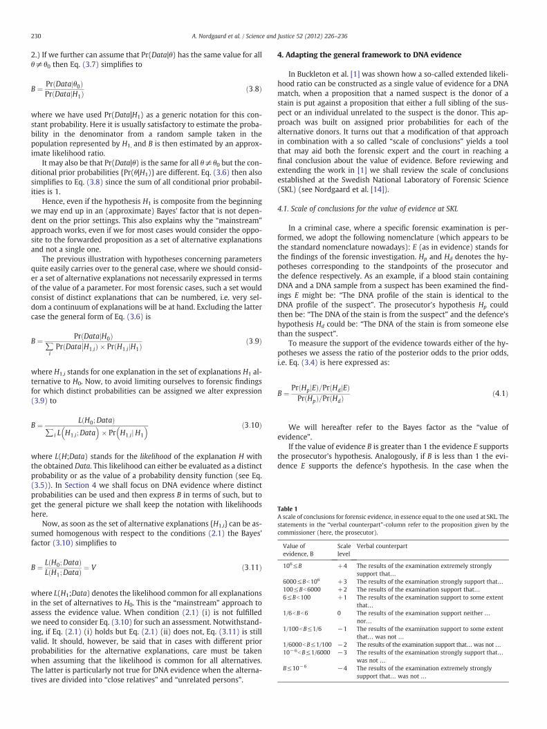
Table 1A scale of conclusions for forensic evidence, in essence equal to the one used at SKL. Thestatements in the “verbal counterpart”-column refer to the proposition given by thecommissioner (here, the prosecutor).
Value ofevidence, B
Scalelevel
Verbal counterpart
106≤B +4 The results of the examination extremely stronglysupport that…
6000≤Bb106 +3 The results of the examination strongly support that…100≤Bb6000 +2 The results of the examination support that…6≤Bb100 +1 The results of the examination support to some extent
that…1/6bBb6 0 The results of the examination support neither …
nor…1/100bB≤1/6 −1 The results of the examination support to some extent
that… was not …1/6000bB≤1/100 −2 The results of the examination support that…was not…10−6bB≤1/6000 −3 The results of the examination strongly support that…
was not …B≤10−6 −4 The results of the examination extremely strongly
support that… was not …
230 A. Nordgaard et al. / Science and Justice 52 (2012) 226–236
2.) If we further can assume that Pr(Data|θ) has the same value for allθ≠θ0 then Eq. (3.7) simplifies to
B ¼ PrðData θ0j ÞPrðData H1j Þ ð3:8Þ
where we have used Pr(Data|H1) as a generic notation for this con-stant probability. Here it is usually satisfactory to estimate the proba-bility in the denominator from a random sample taken in thepopulation represented by H1, and B is then estimated by an approx-imate likelihood ratio.
It may also be that Pr(Data|θ) is the same for all θ≠θ0 but the con-ditional prior probabilities {Pr(θ|H1)} are different. Eq. (3.6) then alsosimplifies to Eq. (3.8) since the sum of all conditional prior probabil-ities is 1.
Hence, even if the hypothesis H1 is composite from the beginningwe may end up in an (approximate) Bayes' factor that is not depen-dent on the prior settings. This also explains why the “mainstream”
approach works, even if we for most cases would consider the oppo-site to the forwarded proposition as a set of alternative explanationsand not a single one.
The previous illustration with hypotheses concerning parametersquite easily carries over to the general case, where we should consid-er a set of alternative explanations not necessarily expressed in termsof the value of a parameter. For most forensic cases, such a set wouldconsist of distinct explanations that can be numbered, i.e. very sel-dom a continuum of explanations will be at hand. Excluding the lattercase the general form of Eq. (3.6) is
where H1,i stands for one explanation in the set of explanations H1 al-ternative to H0. Now, to avoid limiting ourselves to forensic findingsfor which distinct probabilities can be assigned we alter expression(3.9) to
B ¼ L H0;Datað Þ∑i L H1;i;Data
� �� Pr H1;ijH1
� � ð3:10Þ
where L(H;Data) stands for the likelihood of the explanation H withthe obtained Data. This likelihood can either be evaluated as a distinctprobability or as the value of a probability density function (see Eq.(3.5)). In Section 4 we shall focus on DNA evidence where distinctprobabilities can be used and then express B in terms of such, but toget the general picture we shall keep the notation with likelihoodshere.
Now, as soon as the set of alternative explanations {H1,i} can be as-sumed homogenous with respect to the conditions (2.1) the Bayes'factor (3.10) simplifies to
B ¼ L H0;Datað ÞL H1;Datað Þ ¼ V ð3:11Þ
where L(H1;Data) denotes the likelihood common for all explanationsin the set of alternatives to H0. This is the “mainstream” approach toassess the evidence value. When condition (2.1) (i) is not fulfilledwe need to consider Eq. (3.10) for such an assessment. Notwithstand-ing, if Eq. (2.1) (i) holds but Eq. (2.1) (ii) does not, Eq. (3.11) is stillvalid. It should, however, be said that in cases with different priorprobabilities for the alternative explanations, care must be takenwhen assuming that the likelihood is common for all alternatives.The latter is particularly not true for DNA evidence when the alterna-tives are divided into “close relatives” and “unrelated persons”.
4. Adapting the general framework to DNA evidence
In Buckleton et al. [1] was shown how a so-called extended likeli-hood ratio can be constructed as a single value of evidence for a DNAmatch, when a proposition that a named suspect is the donor of astain is put against a proposition that either a full sibling of the sus-pect or an individual unrelated to the suspect is the donor. This ap-proach was built on assigned prior probabilities for each of thealternative donors. It turns out that a modification of that approachin combination with a so called “scale of conclusions” yields a toolthat may aid both the forensic expert and the court in reaching afinal conclusion about the value of evidence. Before reviewing andextending the work in [1] we shall review the scale of conclusionsestablished at the Swedish National Laboratory of Forensic Science(SKL) (see Nordgaard et al. [14]).
4.1. Scale of conclusions for the value of evidence at SKL
In a criminal case, where a specific forensic examination is per-formed, we adopt the following nomenclature (which appears to bethe standard nomenclature nowadays): E (as in evidence) stands forthe findings of the forensic investigation. Hp and Hd denotes the hy-potheses corresponding to the standpoints of the prosecutor andthe defence respectively. As an example, if a blood stain containingDNA and a DNA sample from a suspect has been examined the find-ings E might be: “The DNA profile of the stain is identical to theDNA profile of the suspect”. The prosecutor's hypothesis Hp couldthen be: “The DNA of the stain is from the suspect” and the defence'shypothesis Hd could be: “The DNA of the stain is from someone elsethan the suspect”.
To measure the support of the evidence towards either of the hy-potheses we assess the ratio of the posterior odds to the prior odds,i.e. Eq. (3.4) is here expressed as:
B ¼ PrðHp Ej Þ=PrðHd Ej ÞPrðHpÞ=Pr Hdð Þ ð4:1Þ
We will hereafter refer to the Bayes factor as the “value ofevidence”.
If the value of evidence B is greater than 1 the evidence E supportsthe prosecutor's hypothesis. Analogously, if B is less than 1 the evi-dence E supports the defence's hypothesis. In the case when the
231A. Nordgaard et al. / Science and Justice 52 (2012) 226–236
value of evidence is equal to 1 the evidence gives no increased sup-port to either of the hypotheses.
A scale of conclusions in essence equal to the one established atSKL [14] for reporting the value of evidence is shown in Table 1. Ithas nine “levels”, −4 to +4, of which level +1 to level +4 representan increasing support of the prosecutor's hypothesis while −1 to −4represent an increasing support of the defence's hypothesis, with−4as the strongest support for the defence's hypothesis. Level 0 isobtained when the findings E gives approximately equal support toeither of the hypotheses.
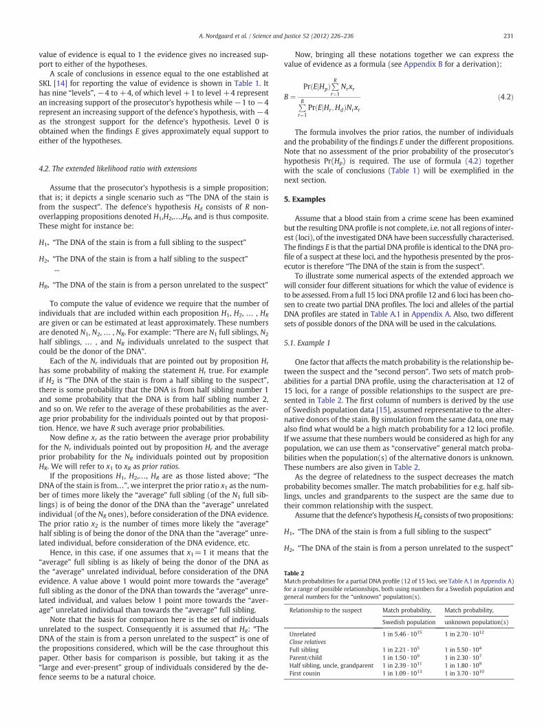
Table 2Match probabilities for a partial DNA profile (12 of 15 loci, see Table A.1 in Appendix A)for a range of possible relationships, both using numbers for a Swedish population andgeneral numbers for the “unknown” population(s).
Relationship to the suspect Match probability, Match probability,
Swedish population unknown population(s)
Unrelated 1 in 5.46·1015 1 in 2.70·1012
Close relativesFull sibling 1 in 2.21·105 1 in 5.50·104
Parent/child 1 in 1.50·109 1 in 2.30·107
Half sibling, uncle, grandparent 1 in 2.39·1011 1 in 1.80·109
First cousin 1 in 1.09·1013 1 in 3.70·1010
4.2. The extended likelihood ratio with extensions
Assume that the prosecutor's hypothesis is a simple proposition;that is; it depicts a single scenario such as “The DNA of the stain isfrom the suspect”. The defence's hypothesis Hd consists of R non-overlapping propositions denoted H1,H2,…,HR, and is thus composite.These might for instance be:
H1. “The DNA of the stain is from a full sibling to the suspect”
H2. “The DNA of the stain is from a half sibling to the suspect”...
HR. “The DNA of the stain is from a person unrelated to the suspect”
To compute the value of evidence we require that the number ofindividuals that are included within each proposition H1, H2, … , HR
are given or can be estimated at least approximately. These numbersare denoted N1, N2,… , NR. For example: “There are N1 full siblings, N2
half siblings, … , and NR individuals unrelated to the suspect thatcould be the donor of the DNA”.
Each of the Nr individuals that are pointed out by proposition Hr
has some probability of making the statement Hr true. For exampleif H2 is “The DNA of the stain is from a half sibling to the suspect”,there is some probability that the DNA is from half sibling number 1and some probability that the DNA is from half sibling number 2,and so on. We refer to the average of these probabilities as the aver-age prior probability for the individuals pointed out by that proposi-tion. Hence, we have R such average prior probabilities.
Now define xr as the ratio between the average prior probabilityfor the Nr individuals pointed out by proposition Hr and the averageprior probability for the NR individuals pointed out by propositionHR. We will refer to x1 to xR as prior ratios.
If the propositions H1, H2,…, HR are as those listed above; “TheDNA of the stain is from…”, we interpret the prior ratio x1 as the num-ber of times more likely the “average” full sibling (of the N1 full sib-lings) is of being the donor of the DNA than the “average” unrelatedindividual (of the NR ones), before consideration of the DNA evidence.The prior ratio x2 is the number of times more likely the “average”half sibling is of being the donor of the DNA than the “average” unre-lated individual, before consideration of the DNA evidence, etc.
Hence, in this case, if one assumes that x1=1 it means that the“average” full sibling is as likely of being the donor of the DNA asthe “average” unrelated individual, before consideration of the DNAevidence. A value above 1 would point more towards the “average”full sibling as the donor of the DNA than towards the “average” unre-lated individual, and values below 1 point more towards the “aver-age” unrelated individual than towards the “average” full sibling.
Note that the basis for comparison here is the set of individualsunrelated to the suspect. Consequently it is assumed that HR: “TheDNA of the stain is from a person unrelated to the suspect” is one ofthe propositions considered, which will be the case throughout thispaper. Other basis for comparison is possible, but taking it as the“large and ever-present” group of individuals considered by the de-fence seems to be a natural choice.
Now, bringing all these notations together we can express thevalue of evidence as a formula (see Appendix B for a derivation):
B ¼PrðEjHpÞ
PRr¼1
Nrxr
PRr¼1
Pr E Hr ;Hdj ÞNrxrðð4:2Þ
The formula involves the prior ratios, the number of individualsand the probability of the findings E under the different propositions.Note that no assessment of the prior probability of the prosecutor'shypothesis Pr(Hp) is required. The use of formula (4.2) togetherwith the scale of conclusions (Table 1) will be exemplified in thenext section.
5. Examples
Assume that a blood stain from a crime scene has been examinedbut the resulting DNA profile is not complete, i.e. not all regions of inter-est (loci), of the investigated DNA have been successfully characterised.The findings E is that the partial DNA profile is identical to the DNA pro-file of a suspect at these loci, and the hypothesis presented by the pros-ecutor is therefore “The DNA of the stain is from the suspect”.
To illustrate some numerical aspects of the extended approach wewill consider four different situations for which the value of evidence isto be assessed. From a full 15 loci DNA profile 12 and 6 loci has been cho-sen to create two partial DNA profiles. The loci and alleles of the partialDNA profiles are stated in Table A.1 in Appendix A. Also, two differentsets of possible donors of the DNA will be used in the calculations.
5.1. Example 1
One factor that affects the match probability is the relationship be-tween the suspect and the “second person”. Two sets of match prob-abilities for a partial DNA profile, using the characterisation at 12 of15 loci, for a range of possible relationships to the suspect are pre-sented in Table 2. The first column of numbers is derived by the useof Swedish population data [15], assumed representative to the alter-native donors of the stain. By simulation from the same data, one mayalso find what would be a high match probability for a 12 loci profile.If we assume that these numbers would be considered as high for anypopulation, we can use them as “conservative” general match proba-bilities when the population(s) of the alternative donors is unknown.These numbers are also given in Table 2.
As the degree of relatedness to the suspect decreases the matchprobability becomes smaller. The match probabilities for e.g. half sib-lings, uncles and grandparents to the suspect are the same due totheir common relationship with the suspect.
Assume that the defence's hypothesisHd consists of two propositions:
H1. “The DNA of the stain is from a full sibling to the suspect”
H2. “The DNA of the stain is from a person unrelated to the suspect”
Prior ratio, x(Full sibling versus "average" unrelated)
Val
ue o
f evi
denc
e, B
1 10000 20000 30000 40000 50000
+1
+2
+3
+4
28370
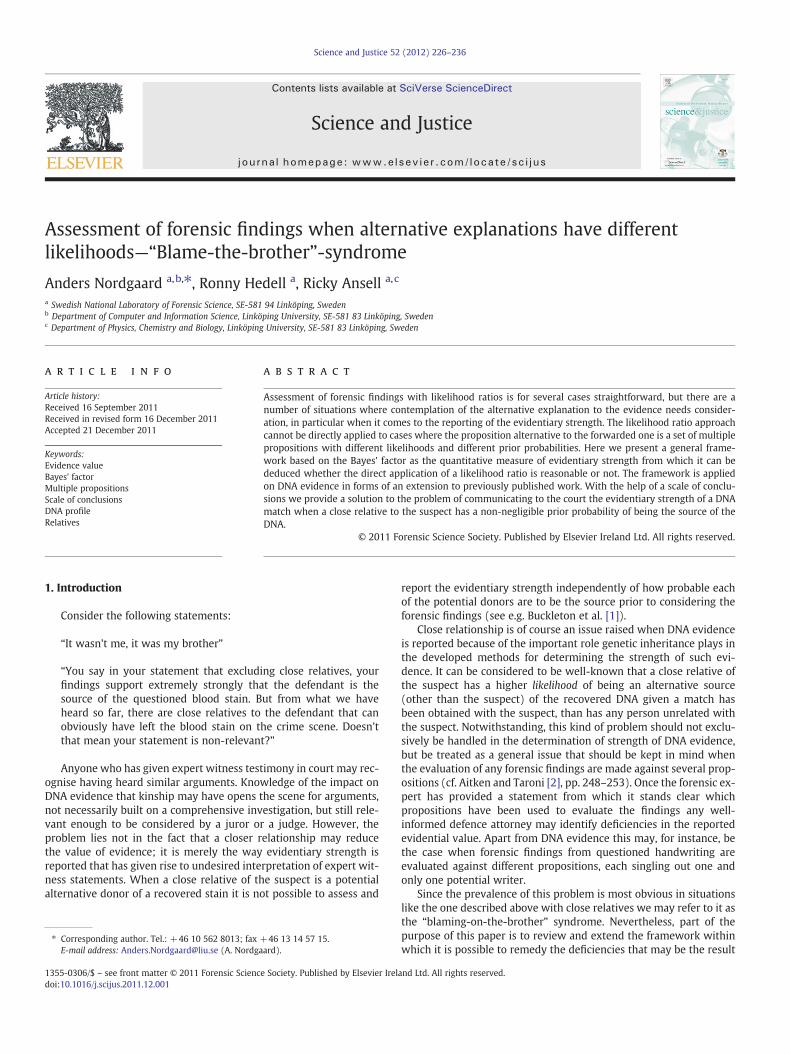
Min
Fig. 1. The value of evidence B in relation to the prior ratio x expressing how manytimes more likely the full sibling is of being the donor of the DNA than the “average”unrelated individual (of the 100,000), before consideration of the findings E. Limitsfor level +1 to +4 of the scale of conclusions are marked in the figure, as well asthe lowest possible value of evidence (“Min”). Note the logarithmic scale of the verticalaxis. For this example a partial DNA-profile with the characterisation at 12 of 15 loci isused.
232 A. Nordgaard et al. / Science and Justice 52 (2012) 226–236
Suppose that one full sibling to the suspect and 100,000 unrelatedindividuals are proposed as possible donors of the DNA (Table 3).
Since the only close relative to the suspect considered is a full sib-ling, there is only one prior ratio to consider; the one that expresshow much more likely the full sibling is of being the donor of theDNA than the “average” unrelated individual (of the 100,000), beforeconsideration of the findings E. We denote this prior ratio simply as x.
To incorporate the concept of match probability into the calcula-tions of the value of evidence we make a slight modification of Eq.(4.2) (see formula (A.4) in Appendix B). The formula for the valueof evidence as a function of the prior ratio x can then be expressed as:
B ¼ xþ 100;000x
2:21⋅105 þ100;0005:46⋅1015
ð5:1Þ
using the match probabilities from the Swedish population data. Anillustration of how the value of evidence B changes with the priorratio x is given in Fig. 1. The scale of the vertical axis in this figure islogarithmic, with only the limits for the level +1 to level +4 conclu-sions marked. As x becomes larger the value of evidence becomessmaller and the theoretical lower limit of the value of evidence,221,000 labelled in the figure as “Min” (for minimum), is obtainedwhen x goes to infinity. The range of x in this figure has been restrict-ed to the interval 1 to 50,000 since that interval captures the most in-formative results. When x is set to approximately 28,370 or below thevalue of evidence is above one million, which corresponds to level +4on the scale of conclusions. If x is greater than or equal to 28,370 thevalue of evidence is below one million and above 221,000, corre-sponding to level +3. A summary of the main results is given inTable 4. Hence, if one can settle that the full sibling is more than,roughly, 28 thousand times more likely of being the donor of theDNA than the “average” unrelated individual, before considerationof the findings E, one would obtain a conclusion of level +3, other-wise a conclusion of level +4.
For comparison, if the number of unrelated individuals is insteadset to 50,000, the breakpoint between level +4 and level +3 is not28,370 but 14,185. If 10,000 unrelated individuals are proposed as do-nors of the DNA the breakpoint is about 2837.
If the representativeness of the Swedish population data used can-not be justified, the match probabilities corresponding to the “un-known” population(s) may be adopted into the calculations. In thatcase the breakpoint between level +4 and level +3 is instead ap-proximately 5820 (see Table 5).
5.2. Example 2
For this example, with the same 12 loci profile as in Example 1,more close relatives to the suspect than just the full sibling arebeing included as possible donors of the DNA. The number of unre-lated individuals and close relatives considered are stated in Table 6.
There are four prior ratios to consider; howmuchmore likely the fullsibling, the “average” parent/child, the “average” half sibling/uncle/grandparent and the “average” first cousin is of being the donor of the
Table 3Number of possible donors of the crime scene DNA other than the suspect, for Examples 1and 3.
Relationship to the suspect Number of individuals
Unrelated 100,000Close relativesFull sibling 1
DNA than the “average” unrelated individual, before consideration ofthe findings E. These prior ratios are denoted x1, x2, x3 and x4 respectively.
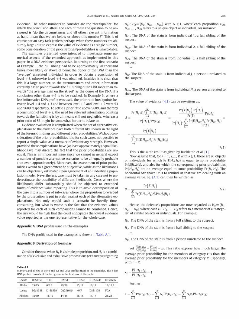
By introducing more variables the situation gets more complexand harder to visualise and communicate. If one can e.g. assumethat the prior ratios for the different groups of close relatives areequal to each other, i.e. if x1=x2=x3=x4=x, the complexity is re-duced. This might be a reasonable approach in those cases wherethe circumstances point no more towards one of the defence's prop-ositions than to another. If so, the value of evidence B can beexpressed as:
B ¼ x 1þ 2þ 5þ 8ð Þ þ 100;000
x 12:21⋅105 þ 2
1:50⋅109 þ 52:39⋅1011 þ 8
1:09⋅1013
� �þ 100;000
5:46⋅1015ð5:2Þ
using the match probabilities of the Swedish population. Table 7 pre-sents the main results of this example. No matter how large we set x,we never obtain a value of B below one million, i.e. the value of evi-dence will always yield a conclusion of level +4, in contrast to Exam-ple 1 where a conclusion of level +3 was obtained when the priorratio was greater than approximately 28,370. When x increases,more and more “belief” of being the donor of the DNA is assignednot only to the full sibling but also to the more distant “average”close relatives, of which the corresponding match probabilities aremuch smaller than the match probability of the full sibling. Therefore,the minimum value of B is also larger in this case.
Table 4Summary of the main results for Example 1 using the match probabilities of theSwedish population.
Value ofevidence,B
Prior ratio, x(Full sibling versus “average” unrelated)
+4 Less than 28,370+3 Greater than or equal to 28,370
Table 5Summary of the main results for Example 1 using the match probabilities of the“unknown” population(s).
Value ofevidence, B
Prior ratio, x(Full sibling versus “average” unrelated)
+4 Less than 5820+3 Greater than or equal to 5820
Table 7Summary of the main results for Example 2 when all prior ratios are equal to eachother.
Value ofevidence, B
Prior ratio, x(“Average” close relatives versus “average” unrelated)
+4 For all values
Value of evidence, B
ther
"av
erag
e" c
lose
rel
ativ
es"a
vera
ge"
unre
late
d)
1000
10000
1e+05
1e+06
233A. Nordgaard et al. / Science and Justice 52 (2012) 226–236
However, it may be more informative to treat the prior ratio of thefull sibling separately from the other prior ratios. That is, we denote x1as x and set x2=x3=x4=y. The formula for the value of evidence be-comes:
B ¼ xþ y 2þ 5þ 8ð Þ þ 100;000x
2:21⋅105 þ y 21:50⋅109 þ 5
2:39⋅1011 þ 81:09⋅1013
� �þ 100;000
5:46⋅1015
ð5:3Þ
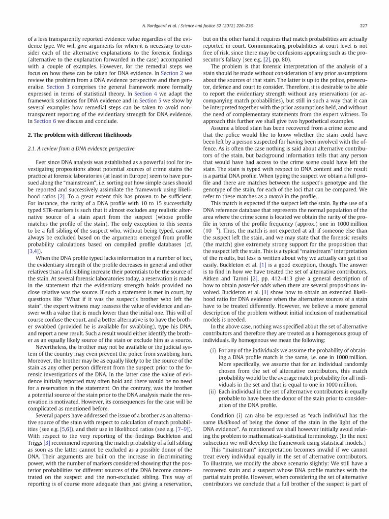
By assessing the value of evidence (5.3) for different values of theprior ratios x and ywe obtain the results presented in Fig. 2. On the x-axis is the prior ratio for the full sibling versus the “average” unre-lated individual. On the y-axis is the prior ratio for the “average”close relatives (except for the full sibling) versus the “average” unre-lated individual. The darker the colour in the figure, the higher is thevalue of evidence. The solid line indicates the border between a level+3 result and a level +4 result.
The dashed line in Fig. 2 represents the case when the prior ratiosx and y are taken as equal to each other, i.e. when the prior ratios forall the groups of close relatives to the suspect are equal;x1=x2=x3=x4=x. This scenario was examined above in Table 7.
From Fig. 2 we see that a conclusion of level +3 is attainable, if theassumption of equal prior ratios for the full sibling and the other closerelatives is dropped, and if x is quite a bit larger than y. That is, if weare not on the dashed line, in Fig. 2, but in the “+3”-region in the fig-ure. One special case that might be of interest is when y=1, that iswhen the other “average” close relatives (non full siblings) are aslikely as the “average” unrelated individual of being the donor ofthe stain, prior to the findings E. It turns out that, in this case, the min-imum prior ratio x of the full sibling required for a conclusion belowlevel +4 is still about 28 thousand, just as in Example 1.
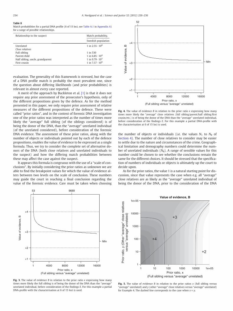
5.3. Example 3
The settings for this example are as in Example 1, but with a lessinformative DNA profile using only the characterisation at 6 of 15loci. The match probabilities are given in Table 8. Note that thematch probabilities are remarkably smaller than before when 12 of15 loci were chosen to create the partial DNA profile.
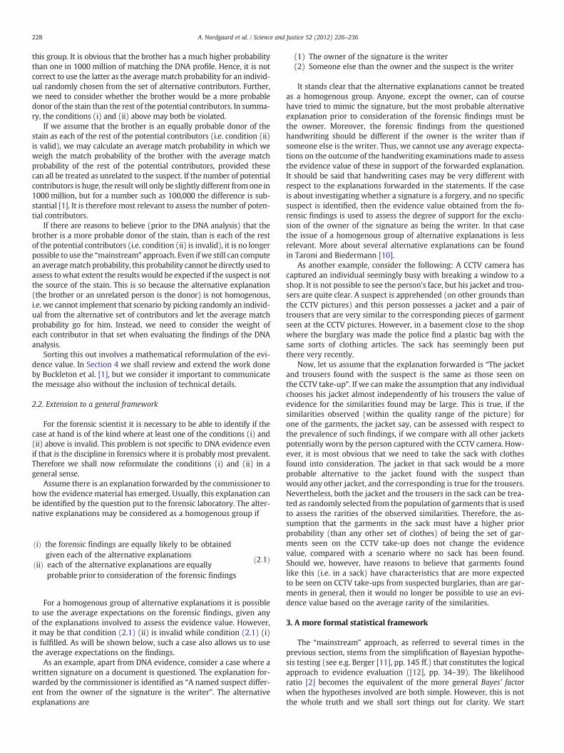
With one full sibling to the suspect and 100,000 unrelated individ-uals as proposed donors of the DNA (Table 3) the value of evidence, inrelation to the prior ratio x, is given in Fig. 3. When x is below 53 aconclusion of level +4 is reached. When x is between 53 and 9689
Table 6Number of possible donors of the crime scene DNA other than the suspect, for Exam-ples 2 and 4.
the conclusion reached is at level +3, while the conclusion remainsat level +2 whenever x is greater than 9689.
5.4. Example 4
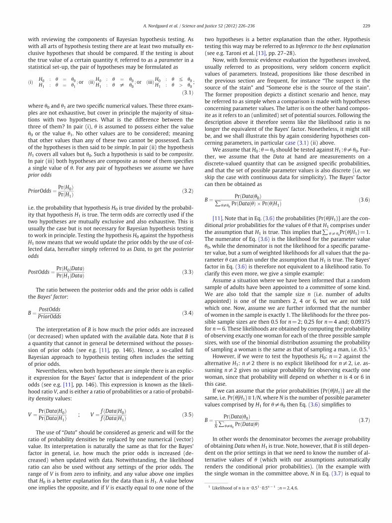
Here, we will use the same DNA profile as in Example 3 (6 of 15loci), but in addition to the full sibling to the suspect we will also in-clude the other close relatives that were considered in Example 2(Table 6). Again, we will first consider the case when all prior ratiosare equal to each other; x1=x2=x3=x4=x. The results are shownin Fig. 4. We see that level +2 is never reached and that level +3 isreached with a somewhat smaller value of x than in Example 3; ap-proximately 52 compared to 53.
If the prior ratio of the full sibling x1=x is held separately from theother prior ratios x2=x3=x4=y, we can consider the approachabove as a special case of the situation illustrated in Fig. 5; the dashedline corresponds to the solid line of Fig. 4. If, for example, both x and yare set to 1 a conclusion of level +4 is obtained. However, also level+3 is attainable when the prior ratio x is equal to 1, but this requiresthat the prior ratio y is set to approximately 4800 or above. A conclu-sion of level +2 is attainable only if the assumption of equal prior ra-tios is dropped and if x is somewhat larger than y.
6. Discussion and conclusions
In this paper we have provided a framework for how differinglikelihoods and differing prior probabilities would affect the Bayes'factor that can be seen as the general quantitative measure of eviden-tiary strength. This framework aids in deducing when the Bayes' fac-tor can be simplified to a likelihood ratio that is addressed as themeasure of evidentiary strength in the logical approach to evidence
Prior ratio, x(Full sibling versus "average" unrelated)
Prio
r ra
tio, y
(O
vers
us
1 10 100 1000 10000 1e+05 1e+061
10
100
Fig. 2. The value of evidence B in relation to the prior ratios x (full sibling versus“average unrelated”) and y (other “average” close relatives versus “average” unrelated)for Example 2. The dashed line corresponds to the case when x=y. Note the logarithmicscales of the axes.
Table 8Match probabilities for a partial DNA profile (6 of 15 loci, see Table A.1 in Appendix A)for a range of possible relationships.
Relationship to the suspect Match probability,
Swedish population
Unrelated 1 in 2.55·108
Close relativesFull sibling 1 in 530Parent/child 1 in 6.85·104
Half sibling, uncle, grandparent 1 in 9.79·105
First cousin 1 in 7.57·106
Prior ratio, x(Full sibling versus "average" unrelated)
Val
ue o
f evi
denc
e, B
1 4000 8000 12000 16000
+1
+2
+3
+4
52
Min
Fig. 4. The value of evidence B in relation to the prior ratio x expressing how manytimes more likely the “average” close relatives (full sibling/parent/half sibling/firstcousin/etc.) is of being the donor of the DNA than the “average” unrelated individual,before consideration of the findings E. For this example a partial DNA-profile withthe characterisation at 6 of 15 loci is used.
234 A. Nordgaard et al. / Science and Justice 52 (2012) 226–236
evaluation. The generality of this framework is stressed, but the caseof a DNA profile match is probably the most prevalent one, sincethe question about differing likelihoods (and prior probabilities) isrelevant in almost every case reported.
A merit of the approach by Buckleton et al. [1] is that it does notrequire any prior assessment of the prosecutor's hypothesis, only ofthe different propositions given by the defence. As for the methodpresented in this paper, we only require prior assessment of relativemeasures of the different propositions of the defence. These werecalled “prior ratios”, and in the context of forensic DNA investigationone of the prior ratios was interpreted as the number of times morelikely the “average” full sibling (of the siblings considered) is ofbeing the donor of the DNA, than the “average” unrelated individual(of the unrelated considered), before consideration of the forensicDNA evidence. The assessment of these prior ratios, along with thenumber of objects or individuals pointed out by each of the defencepropositions, enables the value of evidence to be expressed as a singleformula. Thus, we try to consider the complete set of alternative do-nors of the DNA (both close relatives and unrelated individuals tothe suspect) and how the differing match probabilities betweenthese may affect the case against the suspect.
It appears this formula is congruous with the use of a “scale of con-clusions”. By initially considering the prior ratios as unknown we areable to find the breakpoint values for which the value of evidence al-ters between two levels on the scale of conclusion. These numbersmay guide the court in reaching a final conclusion regarding thevalue of the forensic evidence. Care must be taken when choosing
Val
ue o
f evi
denc
e, B
1 4000 8000 12000 16000
+1
+2
+3
+4
53 9689
Min
Prior ratio, x(Full sibling versus "average" unrelated)
Fig. 3. The value of evidence B in relation to the prior ratio x expressing how manytimes more likely the full sibling is of being the donor of the DNA than the “average”unrelated individual, before consideration of the findings E. For this example a partialDNA-profile with the characterisation at 6 of 15 loci is used.
the number of objects or individuals (i.e. the values N1 to NR ofSection 4). The number of close relatives to consider may be easierto settle due to the nature and circumstances of the crime. Geograph-ical limitation and demography numbers could determine the num-ber of unrelated individuals (NR). A range of sensible values for thisnumber could be chosen to see whether the conclusions remain thesame for the different choices. It should be stressed that the specifica-tion of numbers of individuals or objects is ultimately up the court todecide upon.
As for the prior ratios, the value 1 is a natural starting point for dis-cussion, since that value represents the case when e.g. all “average”close relatives are as likely as the “average” unrelated individual ofbeing the donor of the DNA, prior to the consideration of the DNA
Value of evidence, B
Prior ratio, x(Full sibling versus "average" unrelated)
Prio
r ra
tio, y
(O
ther
"av
erag
e" c
lose
rel
ativ
esve
rsus
"av
erag
e" u
nrel
ated
)
1 10 100 1000 10000 1e+051
10
100
1000
10000
1e+05
Fig. 5. The value of evidence B in relation to the prior ratios x (full sibling versus“average” unrelated) and y (other “average” close relatives versus “average” unrelated)for Example 4. The dashed line corresponds to the case when x=y.
235A. Nordgaard et al. / Science and Justice 52 (2012) 226–236
evidence. The other numbers to consider are the “breakpoints” forwhich the conclusion alters. For each of these the question to be an-swered is “do the circumstances and all other relevant informationat hand mean that we are below or above this number?”. This is ofcourse not an easy task (unless perhaps when these numbers are ab-surdly large) but to express the value of evidence as a single number,some consideration of the prior settings/probabilities is unavoidable.
The examples presented were intended to investigate some nu-merical aspects of the extended approach, as implemented in thispaper, in a DNA evidence perspective. Returning to the first scenarioof Example 1, the full sibling had to be approximately 28 thousandtimes more likely or above of being the donor of the DNA than the“average” unrelated individual in order to obtain a conclusion oflevel +3, otherwise level +4 was obtained. Intuitive it is clear thatthis is a large number, so the circumstances and other informationcertainly has to point towards the full sibling quite a bit more than to-wards “the average man on the street” as the donor of the DNA, if aconclusion other than +4 is to be reached. In Example 3, where aless informative DNA profile was used, the prior ratio breakpoints be-tween level +4 and +3 and between level +3 and level +2 were 53and 9689 respectively. To settle a prior ratio above 9689, and therebya conclusion of level +2, the need for relevant information pointingtowards the full sibling is by all means still not negligible, whereas aprior ratio of 53 might be somewhat harder to relate to.
Evidence evaluation is complicated when the set of alternative ex-planations to the evidence have both different likelihoods in the lightof the forensic findings and different prior probabilities. Without con-sideration of the prior probabilities it is, for such cases, not possible toreport a single value as a measure of evidentiary strength. However,provided these explanations have (at least approximately) equal like-lihoods we may discard the fact that the prior probabilities are un-equal. This is an important issue since we cannot in general expecta number of possible alternative scenarios to be all equally probable(not even approximately). Moreover, the assessment of prior proba-bilities would to a great extent be subjective, while as the likelihoodscan be objectively estimated upon agreement of an underlying popu-lation model. Nevertheless, care must be taken in any case not to un-derestimate the possibility of different likelihoods. Cases where thelikelihoods differ substantially should be objected to extendedforms of evidence value reporting. This is to avoid decomposition ofthe case into a number of sub-cases where the proposition forwardedby the prosecution is put in order against each of the alternative ex-planations. Not only would such a scenario be heavily time-consuming, but what is worse is the fact that the evidence valuesreported for each of such comparisons cannot be combined. Hence,the risk would be high that the court anticipates the lowest evidencevalue reported as the one representative for the whole case.
Appendix A. DNA profile used in the examples
The DNA profile used in the examples is shown in Table A.1.
Appendix B. Derivation of formulas
Consider the case whenHp is a simple proposition andHd is a combi-nation ofN exclusive and exhaustive propositions (exhaustive regarding
Table A.1Markers and alleles of the 6 and 12 loci DNA profiles used in the examples. The 6 lociDNA profile consists of the loci given in the first row of the table.
Hd); Hd={Hd1,Hd2,…,HdN} with N ≥1, where each proposition Hd1,Hd2, … , HdN refers to a unique object or individual. For instance:
Hd1. The DNA of the stain is from individual 1, a full sibling of thesuspect.
Hd2. The DNA of the stain is from individual 2, a full sibling of thesuspect.
Hd3. The DNA of the stain is from individual 3, a half sibling of thesuspect
...
Hdj. The DNA of the stain is from individual j, a person unrelated tothe suspect
...
HdN. The DNA of the stain is from individual N, a person unrelated tothe suspect.
The value of evidence (4.1) can be rewritten as:
B ¼PrðHp Ej Þ=
XN
i¼1
PrðHdi;Hd Ej Þ
Pr Hp
� �=Pr Hdð Þ
¼
PrðE Hp
����Pr Hp
� �
Pr Eð Þ ⋅Pr Hdð Þ
Pr Hp
� �⋅XN
i¼1
PrðE Hdi;Hdj ÞPr Hdi;Hdð ÞPr Eð Þ
¼
¼PrðE Hp
����
XN
i¼1
Pr E Hdi;Hdj ÞPr Hdi Hdj Þðð
ðA:1ÞThis is the same result as given by Buckleton et al. [1].Now assume that, for r=1, 2,…, R with R≥1, there are Nr objects
or individuals for which Pr(E|Hdi,Hd) is equal to some probabilityPr(E|Hr,Hd), and also for which the corresponding prior probabilitiesPr(Hdi|Hd) are on average equal to some probability Pr Hr Hdj Þð . Thehorizontal bar above Pr is to remind us that we are dealing with anaverage value. Eq. (A.1) can then be written as:
B ¼PrðE Hp
����
PRr¼1
Pr E Hr ;Hdj ÞNrPr Hr Hdj Þð� ðA:2Þ
Hence, the defence's propositions are now regarded as Hd={H1,H2,…,HR}, where each H1, H2, … , HR refers to a member of a “catego-ry” of similar objects or individuals. For example;
H1. The DNA of the stain is from a full sibling to the suspect,
H2. The DNA of the stain is from a half sibling to the suspect...
HR. The DNA of the stain is from a person unrelated to the suspect
Set PrðHr Hdj ÞPrðHR Hdj Þ ¼
Pr Hrð ÞPrðHRÞ
¼ xr . This ratio express how much larger the
average prior probability for the members of category r is than theaverage prior probability for the members of category R. Especially,with r=R:
xR ¼ PrðHR Hdj ÞPrðHR Hdj Þ ¼ 1
Further:
1 ¼XN
i¼1
PrðHdi Hdj Þ ¼XR
r¼1
NrPrðHr Hdj Þ ¼XR
r¼1
NrxrPr HR Hdj Þ:ð
236 A. Nordgaard et al. / Science and Justice 52 (2012) 226–236
So PrðHR Hdj Þ ¼ 1PRr¼1
Nrxr
, which implies that PrðHr Hdj Þ ¼ xrPRr¼1
Nrxr
.
Hence, Eq. (A.2) can be expressed as:
B ¼PrðE Hp
���� PR
r¼1Nrxr
PRr¼1
Pr E Hr ;Hdj ÞNrxrððA:3Þ
In the context of DNA investigation; assume that a trace contain-ing DNA from a crime scene and a DNA sample from a suspect areto be examined. GS denotes the yet unknown DNA profile of the sus-pect and GC denotes the unknown DNA profile of the trace. After per-forming the DNA typing the finding is E: The DNA profile of the traceand the profile of the suspect are both equal to DNA profile g. In otherwords E is equal to the joint events GS=g and GC=g. Following Evettand Weir [16] (pp. 22–26):
The actual DNA profile of the suspect does not depend on who leftthe stain so:
Pr GS ¼ g Hp
����¼ Pr GS ¼ g Hr;Hdj Þð
�
Further, if the prosecutor's hypothesis is Hp: “The DNA of the traceis from the suspect” and the DNA typing is without errors then:
Pr GC ¼ g GS ¼ g;Hp
����¼ 1
�
Now, Eq. (A.3) may be written as:
B ¼
PRr¼1
Nrxr
PRr¼1
Pr GC ¼ g GS ¼ g;Hr ;Hdj ÞNrxrððA:4Þ
Pr(GC=g|GS=g,Hr,Hd) is what we refer to as a match probability[5].
References
[1] J.S. Buckleton, C.M. Triggs, C. Champod, An extended likelihood ratio frameworkfor interpreting evidence, Science & Justice 46 (2006) 69–78.
[2] C.G.G. Aitken, F. Taroni, Statistics and the Evaluation of Evidence for ForensicScientists, second ed. Wiley, Chichester, 2004.
[3] J. Buckleton, C.M. Triggs, Relatedness and DNA: are we taking it seriously enough?Forensic Science International 152 (2005) 115–119.
[4] J. Buckleton, C. Triggs, The effect of linkage on the calculation of DNA matchprobabilities for siblings and half siblings, Forensic Science International 160(2006) 193–199.
[5] D.J. Balding, R.A. Nichols, DNA profile match probability calculation: how to allowfor population stratification, relatedness, database selection and single bands,Forensic Science International 64 (1994) 125–140.
[6] A.D. Anderson, B.S. Weir, It was one of my brothers, International Journal of LegalMedicine 120 (2006) 95–104.
[7] I.W. Evett, Evaluating DNA profiles in a case where the defence is “It was mybrother”, Journal of the Forensic Science Society 32 (1992) 5–14.
[8] C.H. Brenner, Forensic Genetics: Mathematics, Encyclopedia of Life Sciences, JohnWiley & Sons Ltd, 2006.
[9] R. Puch-Solis, S. Pope, I. Evett, Calculating likelihood ratios for a mixed DNAprofile when a contribution from a genetic relative of a suspect is proposed,Science & Justice 50 (2010) 205–209.
[10] F. Taroni, A. Biedermann, Inadequacies for posterior probabilities for theassessment of scientific evidence, Law, Probability and Risk 4 (2005) 89–114.
[11] J.O. Berger, Statistical Decision Theory and Bayesian Analysis, second ed.Springer-Verlag, New York, 1985.
[12] J. Buckleton, A framework for interpreting evidence, in: J. Buckleton, C.M. Triggs,S.J. Walsh (Eds.), Forensic DNA Evidence Interpretation, CRC Press, Boca Raton FL,2005.
[13] F. Taroni, C. Aitken, P. Garbolino, A. Biedermann, Bayesian Networks and Probabi-listic Inference in Forensic Science, Wiley, Chichester, 2006.
[14] A. Nordgaard, R. Ansell, W. Drotz, L. Jaeger, Scale of conclusions for the value ofevidence, Law, Probability and Risk (2011), doi:10.1093/lpr/mgr020.
[15] L. Albinsson, L. Norén, R. Hedell, R. Ansell, Swedish population data andconcordance for the kits PowerPlex® ESX 16 System, PowerPlex® ESI 16 System,AmpFlSTR® NGM™, AmpFlSTR® SGM Plus™ and Investigator ESSplex, ForensicScience International. Genetics 5 (2011) e89–e92.
[16] I.W. Evett, B.S. Weir, Interpreting DNA Evidence—Statistical Genetics for ForensicScientists, Sinauer Associates, Inc., Sunderland, 1998.