Page 1
1 *
This work was supported by the National Aeronautics and Space Administration (NASA) / Goddard Space Flight Center
(GSFC), Greenbelt, MD, USA, Contract NNG04DA01C.
NASA/GSFC, Mission Engineering and Systems Analysis Division, Flight Mechanics Symposium, Greenbelt, MD, Oct. 2005.
ATTITUDE SENSOR PSEUDONOISE*
Joseph A. Hashmall
Scott E. Lennox
a.i.solutions, Inc.
[email protected]
ABSTRACT
Even assuming perfect attitude sensors and gyros, sensor measurements on a vibrating
spacecraft have apparent errors. These apparent sensor errors, referred to as pseudonoise,
arise because gyro and sensor measurements are performed at discrete times. This paper
explains the concept of pseudonoise, quantifies its behavior, and discusses the effect of
vibrations that are nearly commensurate with measurement periods. Although pseudonoise
does not usually affect attitude determination it does affect sensor performance evaluation.
Attitude rates are usually computed from differences between pairs of accumulated
angle measurements at different times and are considered constant in the periods between
measurements. Propagation using these rates does not reproduce exact instantaneous space-
craft attitudes except at the gyro measurement times. Exact sensor measurements will there-
fore be inconsistent with estimates based on the propagated attitude. This inconsistency
produces pseudonoise.
The characteristics of pseudonoise were determined using a simple, one-dimensional
model of spacecraft vibration. The statistical properties of the deviations of measurements
from model truth were determined using this model and a range of different periods of sensor
and rate measurements.
This analysis indicates that the magnitude of pseudonoise depends on the ratio of the
spacecraft vibration period to the time between gyro measurements and can be as much as
twice the amplitude of the vibration. In cases where the vibration period and gyro or sensor
measurement period are nearly commensurate, unexpected changes in pseudonoise occur.
https://ntrs.nasa.gov/search.jsp?R=20050244355 2019-04-14T20:41:57+00:00Z
Page 2
2
INTRODUCTION
Assume that a spacecraft vibrates with a known frequency and amplitude. The model
used here contains three features:
• True sinusoidal angular displacements of unit amplitude and unit frequency. The
angular displacements are sinusoidal.
• Exact measurements of the angular displacement by two sensors. Sensor displacement
measurements are defined by their cadence (number of measurements made in one
vibration period) and a phase of the first displacement measurement used.
• Exact rate measurements by an integrating rate sensor. This sensor provides inte-
grated rates from one rate measurement to the next at a rate sensor cadence and
starting at an initial phase. It is assumed that the integrated rate at the time of each
rate measurement is exactly equal to the true angular displacement at that time. Dis-
placements are estimated from rate measurements by interpolation or extrapolation.
o Interpolated rates are most often used in post-processing when all of the data is
available before processing. In this case, the estimate of the displacement
angle at any time is obtained by linear interpolation of the integrated rates
before and after the time.
o Extrapolated rates are most often used in real time processing when data is
processed in the order in which it is generated. In this case, the estimate of the
displacement angle at any time is obtained by linear extrapolation of the two
most recent integrated rate measurements.
Attitude estimation filters which use rate data attempt to minimize the differences
between the measured displacement and the displacement estimated (by interpolation or
extrapolation) from the rate measurements.
Even with exact measurements, true spacecraft vibrations cause an apparent noise in
the attitude sensor. This noise is referred to as pseudonoise. The present paper describes the
origin and properties of pseudonoise. It arises because the linear interpolation or extrapola-
tion used to estimate displacements is not exact.
Figure 1 illustrates the origin of pseudonoise. In it, the sinusoidal line represents the
true angular displacement of the spacecraft in one dimension. On the sinusoidal line are
circles representing rate sensor measurements of integrated displacements since the previous
measurements. Xs on the sinusoidal line represent attitude sensor measurements of the
angular displacements. All of the measurements are exactly on the line because sensors are
assumed to have no error.
At times other than those of rate measurements, the displacement is obtained either by
interpolation (in the case of post-hoc batch least-squares (BLS) estimators), or by extrapola-
tion (in the case of real-time filters). At the time of the displacement measurement (X), the
extrapolated or interpolated displacement differs from the true measured displacement by a
significant amount. This difference is pseudonoise. It arises solely from the fact that the
function used to interpolate or extrapolate rate measurements (linear in this case) cannot
reproduce the true spacecraft displacement between measurements.
Page 3
3
Figure 1. Illustration of Pseudonoise
CHARACTERIZATION OF PSEUDONOISE
All of the descriptions of pseudonoise in this paper shall be related to a sinusoidal
vibration of unit frequency and unit amplitude. Pseudonoise magnitudes are linear with vibra-
tion amplitude. Characteristics that depend on the vibration frequency can be equivalently
viewed as depending on the rate measurement cadence—the number of rate measurements
that are made in a single vibration period.
It is assumed that the rate measurements and displacement measurements are
independent and exact. Attitude sensor measurements are modeled as the exact displacements
at each time. Rate measurements are constructed from pairs of exact displacement
measurements with rates assumed to be constant between these displacement measurements.
This assumption produces results equivalent to those from a perfect Kalman filter, with zero
sensor weight, starting from an exact initial attitude.
In a simple, 1-dimensional model, the spacecraft vibration may be represented as a
periodic angular displacement described by:
)sin(φθ φ = (1)
where φ is the phase at which the displacement, θ, occurs. In the notation used here, the
phase, φ, is not limited to 2π, but increases without limit. Pseudonoise is given in terms of the
Vibration Phase (deg)
Fra
cti
on
al
Dis
pla
cem
en
t
0 60 120 180 240 300 360
-1
-0.8
-0.4
0.4
0.8
-0.6
-0.2
0
0.2
0.6
1
Rate Measurements
Displacement Interpolated Using Rate
Displacement Extrapolated Using Rate
Displacement Measurement
Displacement Measurement
Apparent Displacement
Measurement Error
Apparent Displacement Measurement Error
Page 4
4
measurement phase, φm, and phases of the two rate measurements, φ0 and φ1, that are used to
compute the expected displacement, by:
expected,mmmp θθφ −= (2)
where
)sin( mm φθ = (3)
( )
)()(
expected, 1
01
011 φφ
φφθθ
θθ −−
−+= mm (4)
Note that for interpolation, φ0 ≤ φm ≤ φ1; whereas, for extrapolation, it is assumed that
(2φ1-φ0) ≥φm ≥φ1.
It is clear from Figure 1 that pseudonoise depends strongly on the cadence of the rate
measurements. The high and low rate limits are considered next.
High Rate Cadence
As the cadence becomes large, the approximation of the rate by linear interpolation or
extrapolation becomes more accurate, and the pseudonoise becomes small. This is the case
for very low frequency vibrations or very high frequency rate measurements. As φ0
approaches φ1:
( )
φθ
φφθθ
d
d≅
−
−
)( 01
01 (5)
and
mm θθ ≅expected, (6)
so the pseudonoise approaches zero, Rate measurements follow the vibration well and
pseudonoise is negligible. This case is illustrated in Figure 2.
Low Rate Cadence
As the cadence becomes small, there are many complete vibrations between any
adjacent pairs of rate measurements. In this case, the vibration is at a high frequency
compared to the rate measurements. As seen in Figure 3, rate measurements are bounded by
the vibration amplitude divided by the relatively long time between measurements. The
calculated rates therefore tend to be small compared to those in the high rate cadence case.
Page 5
5
Figure 2. Pseudonoise with High Rate Cadence (Low Vibration Frequency)
Figure 3. Pseudonoise with Low Rate Cadence (High Vibration Frequency)
In the low rate cadence case, the phase of the displacement measurement can be con-
sidered to be independent of the phase of the rate measurements. The displacements θm and
Vibration Phase (deg)
Fra
cti
on
al
Dis
pla
cem
en
t
-0.2
0.4
-1
-0.8
-0.6
-0.4
0
0.2
0.6
0.8
1
0
Interpolated Displacement Extrapolated Displacement
Apparent Displacement Measurement Error
Displacement Extrapolated Using Rate
Displacement Interpolated Using Rate
3600 7200 10800 14400 18000
Fra
cti
on
al D
isp
lac
em
en
t
Vibration Phase (deg)
0
0.1
0.2
0.3
0.4
0.5
0.6
0.7
0.8
0.9
1
10 20 30 40 50 60 70 80 90 100
Displacement Extrapolated Using Rate
Displacement Measurements
Displacement Extrapolated Using Rate
Rate Measurements
Page 6
6
θm,expected (in Eq. (2)) are uncorrelated, and the uncertainty of their difference is just the root-
sum-square of the uncertainty of the two terms.
The standard deviation of θm is given by:
2
1sin
1
sin22
=≅−
=�
��m
mmm
md
d
n φ
φφφσθ (7)
where the summation is over a large set of n measurements spanning many vibration periods
and the integration is over continuous measurements in a single vibration period.
The standard deviation of θm,expected depends on the phases of the two rate measure-
ments. These phases, φ0 and φ1, can be equivalently represented by φ0 and ∆φ (∆φ = φ1 -φ0 ).
Displacement θm,expected lies on a straight line between the points [φ0 , sinφ0] and [φ1 , sinφ1].
Its standard deviation has been calculated for values of φ0 between 0 and 360 deg and of ∆φ
between 360 to 720 deg. The results are shown in Figure 4. The form of the surface shown is
similar for any complete 360 degree cycle of ∆φ.
Figure 4. Standard Deviation of the Expected Deviation Angle for Interpolated Rates
Page 7
7
Intermediate Rate Cadence
The most interesting cases arise when the rate cadence is similar to the vibration
period. Such cases were studied in the range of rate cadences from 0.1 to 10 times the vibra-
tion period. For each value of cadence, the measured and expected displacements were cal-
culated over a large number of vibration cycles (~1000). The differences between measured
and expected displacements were calculated and the standard deviation of these differences
saved. It was verified that neither the phase of the first rate measurement, nor changes in the
number of cycles affected the results significantly except in the case of resonance as described
below. Any influence from the initial phase is thoroughly averaged out by the large number
of measurements and cycles. The resulting standard deviations are shown in Figure 5.
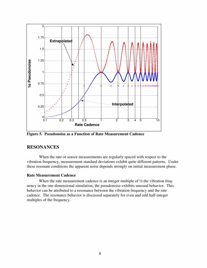
Figure 5 presents several interesting features:
• When the rates are calculated by interpolation
o The standard deviation of the pseudonoise increases with increasing rate meas-
urement cadence until a cadence of about 1, at which point it has a value equal
to the amplitude of the vibration.
o At cadences above 1, the standard deviation of the pseudonoise oscillates with
rate measurement cadence between 1 and roughly 0.8 times the amplitude of
the vibration.
• When the rates are calculated by extrapolation
o The standard deviation of the pseudonoise increases with increasing rate meas-
urement cadence until a cadence of about 0.57, at which it has a value equal to
roughly 1.82 times the amplitude of the vibration.
o At cadences above 0.57, the standard deviation of the pseudonoise oscillates
with rate measurement cadence between 1 and roughly 1.7 times the amplitude
of the vibration. The minima of this oscillation match in cadence and standard
deviation the maxima of the oscillations for interpolated values.
• For both interpolation and extrapolation, the standard deviations form a smooth curve
except at resonance conditions. This smooth curve approaches a standard deviation of
1 as the rate cadence approaches integer values. When the ratio of the vibration
frequency to the cadence is exactly an integer multiple of 0.5, the standard deviation
of the pseudonoise jumps to 1/√2. These singular points are due to resonances and are
discussed below.
Page 8
8
Figure 5. Pseudonoise as a Function of Rate Measurement Cadence
RESONANCES
When the rate or sensor measurements are regularly spaced with respect to the
vibration frequency, measurement standard deviations exhibit quite different patterns. Under
these resonant conditions the apparent noise depends strongly on initial measurement phase.
Rate Measurement Cadence
When the rate measurement cadence is an integer multiple of ½ the vibration freq-
uency in the one dimensional simulation, the pseudonoise exhibits unusual behavior. This
behavior can be attributed to a resonance between the vibration frequency and the rate
cadence. The resonance behavior is discussed separately for even and odd half-integer
multiples of the frequency.
0
0.25
0.5
0.75
1
1.25
1.5
1.75
2
0.1 0.2 0.3 0.5 1 2 3 4 5 10
Rate Cadence
1σσ σσ
Pseu
do
no
ise
Extrapolated
Interpolated
Page 9
9
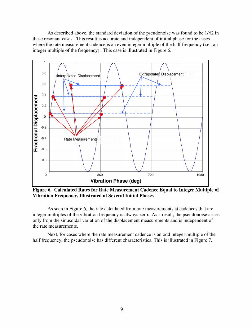
As described above, the standard deviation of the pseudonoise was found to be 1/√2 in
these resonant cases. This result is accurate and independent of initial phase for the cases
where the rate measurement cadence is an even integer multiple of the half frequency (i.e., an
integer multiple of the frequency). This case is illustrated in Figure 6.
Figure 6. Calculated Rates for Rate Measurement Cadence Equal to Integer Multiple of
Vibration Frequency, Illustrated at Several Initial Phases
As seen in Figure 6, the rate calculated from rate measurements at cadences that are
integer multiples of the vibration frequency is always zero. As a result, the pseudonoise arises
only from the sinusoidal variation of the displacement measurements and is independent of
the rate measurements.
Next, for cases where the rate measurement cadence is an odd integer multiple of the
half frequency, the pseudonoise has different characteristics. This is illustrated in Figure 7.
0 360 720 1080
-1
-0.8
-0.6
-0.4
-0.2
0
0.2
0.4
0.6
0.8
1
Vibration Phase (deg)
Extrapolated Displacement Interpolated Displacement
Rate Measurements
Fra
cti
on
al
Dis
pla
ce
me
nt
Page 10
10
Figure 7. Calculated Rates for Rate Measurement Cadence Equal to Odd Integer
Multiple of Half the Vibration Frequency, Illustrated at Two Initial Phases
(Note: The Labels Used in Previous Figures Have Been Eliminated to Avoid Confusion.
The Line Styles and Symbols are Identical to Those in Figure 6.)
When the initial phase is zero, the results are as described above—calculated rates
equal to zero and 1σ pseudonoise equal to 1/√2. At different initial phases, the calculated
rates are not zero and the pseudonoise magnitude varies. Figure 8 shows the pseudonoise
standard deviation as a function of initial phase for the case where the rate measurement
cadence is exactly half of the vibration frequency.
0 360 720 1080
Vibration Phase (deg)
Fra
cti
on
al
Dis
pla
ce
me
nt
-1
-0.8
-0.6
-0.4
-0.2
0
0.2
0.4
0.6
0.8
1
Page 11
11
Figure 8. Pseudonoise Standard Deviation for Rate Measurement Cadence of 0.5,
as a Function of Initial Phase
Displacement Measurement Cadence
If the displacement measurement cadence is an integer multiple of the vibration freq-
uency, all displacement measurements will be made at the same vibration phase. The mean of
the measured displacements will therefore be offset from the mean of the true displacements
by an amount corresponding to the vibrational displacement at the time of each displacement
measurement. This will result in a systematic error in the displacement measurements.
Near Resonance Conditions
When either the rate or displacement measurement cadence is near resonance with the
vibration frequency, the pseudonoise is similar to cases with exact resonance. The significant
difference between exact resonance and near resonance conditions is that in the near reso-
nance conditions the initial phase angle changes slightly in successive cycles whereas the
behavior seen in resonance conditions therefore changes gradually with time—it follows the
behavior of the resonance conditions with varying initial phase.
SIMULATIONS
The effect of pseudonoise was evaluated by simulating a system with pseudonoise and
evaluating the apparent sensor noise. The software used for evaluation of the pseudonoise
0 50 100 150 200 250 300 350 0
0.5
1
1.5
2
2.5
Initial Phase
1σσ σσ
Pseu
do
no
ise
Extrapolated
Interpolated
Page 12
12
was the Multimission Three-Axis Stabilized Spacecraft (MTASS) Attitude Ground Support
System (AGSS). This system has been used operationally on many spacecraft over the last 12
years.
The simulation had the following characteristics:
• Attitude: The simulated attitude included a sinusoidal oscillation on one axis,
imposed on an otherwise constant attitude. The oscillation was generated by the
function:
)sin()( 0ϕωθ += tAt (8)
where θ(t) is the angular displacement on the axis of oscillation at time t, t is the time,
A is the oscillation amplitude, ω is the frequency of oscillation, and ϕ0 is the phase at
time zero. The attitude at time t is a single axis rotation of θ(t). For example, if the
oscillation is about the x-axis:
( )( ) ( )( )( )( ) ( )( )�
��
�
�
���
�
�
−
=
tt
tttM
θθθθ
cossin0
sincos0
001
)( (9)
where M transforms vectors from a geocentric inertial (GCI) frame to the body frame.
• Amplitude: The noise statistics are proportional to the amplitude for small ampli-
tudes. Amplitudes on the order of 10-20 arcsec were used.
• Frequency: The oscillation frequency was π/3 Hertz, where t is in seconds. This
value was chosen because it is irrational and therefore would result in no unintentional
resonances.
• Gyro Cadence: Two sets of gyro cadences were used and the results combined. The
first set was generated so that the base 10 logarithms of the cadences were uniformly
spaced between -1 and 1. This provides a logarithmic spacing of cadences between
0.1 and 10. Since the oscillation frequency chosen was irrational, these cadences do
not intentionally approach resonance.
The second set of cadences were specifically chosen as the oscillation period multi-
plied by a number of values. The values ranged from 0.1 to 1 in steps of 0.1 and
1.5 to 10 in steps of 0.5. This second set was expected to be near resonance with the
oscillation.
• Sensor Observations: Two star trackers were simulated with boresights perpendicu-
lar to the axis about which the oscillation was generated and perpendicular to each
other. In each tracker, five stars were simulated. The positions of the stars in the GCI
frame (reference vectors) were kept constant and the body frame positions (simulated
observations) for the stars at time t were generated by rotating the reference vectors by
the attitude at that time.
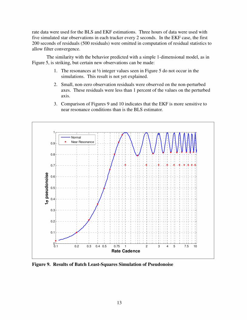
The results of the simulation are shown for two estimation methods. Figure 9 shows a
case where the attitude is determined using a Batch Least-Squares (BLS) estimator. Figure 10
shows a case where the attitude is determined using an Extended Kalman Filter (EKF). For
both estimators, observations were propagated using interpolated rates. Identical sensor and
Page 13
13
rate data were used for the BLS and EKF estimations. Three hours of data were used with
five simulated star observations in each tracker every 2 seconds. In the EKF case, the first
200 seconds of residuals (500 residuals) were omitted in computation of residual statistics to
allow filter convergence.
The similarity with the behavior predicted with a simple 1-dimensional model, as in
Figure 5, is striking, but certain new observations can be made:
1. The resonances at ½ integer values seen in Figure 5 do not occur in the
simulations. This result is not yet explained.
2. Small, non-zero observation residuals were observed on the non-perturbed
axes. These residuals were less than 1 percent of the values on the perturbed
axis.
3. Comparison of Figures 9 and 10 indicates that the EKF is more sensitive to
near resonance conditions than is the BLS estimator.
0.1 0.2 0.3 0.4 0.5 0.75 1 2 3 4 5 7.5 100
0.1
0.2
0.3
0.4
0.5
0.6
0.7
0.8
0.9
1
Rate Cadence
1σσ σσ
ps
eu
do
no
ise
Normal
Near Resonance
Figure 9. Results of Batch Least-Squares Simulation of Pseudonoise
Page 14
14
Figure 10. Results of Extended Kalman Filter Simulation of Pseudonoise (With
Interpolated Rates)
5. Conclusions
Pseudonoise is an interesting phenomenon that seldom has a critical impact on attitude
determination accuracy. Because pseudonoise generally has zero mean, it may influence the
rapidity of filter convergence but will not often significantly influence the accuracy of the
converged solution.
Pseudonoise is most important when the rate measurement cadence is comparable to,
or larger than, the vibration frequency and when the vibration amplitude is large. Cases
where pseudonoise is significant are generally limited by the fact that large amplitude
vibrations seldom occur at high frequency because the total vibration energy increases with
both frequency and amplitude. Examples of spacecraft having vibrations, rate measurement
cadences in the intermediate range described above, and significant vibration amplitudes are
Aqua and ADEOS-II. In both of these missions, the apparent star tracker noise was much
larger than inherent star tracker noise because of pseudonoise.
0.1 0.2 0.3 0.4 0.5 0.75 1 2 3 4 5 7.5 100
0.1
0.2
0.3
0.4
0.5
0.6
0.7
0.8
0.9
1
Rate Cadence
1σσ σσ
ps
eu
do
no
ise
Normal
Near Resonance
Page 15
15
Under some conditions, pseudonoise can affect attitude systems and should be con-
sidered:
• In cases that are near resonance there are amplified effects that can vary slowly with
time.
• In evaluating on-orbit attitude sensor performance, significant portions of apparent
sensor error can arise from pseudonoise.
• The observed uncertainty of sensor measurements is a combination of the true sensor
measurement uncertainty and the pseudonoise. When the pseudonoise is large,
different EKF tuning may be necessary to compute optimal attitudes.