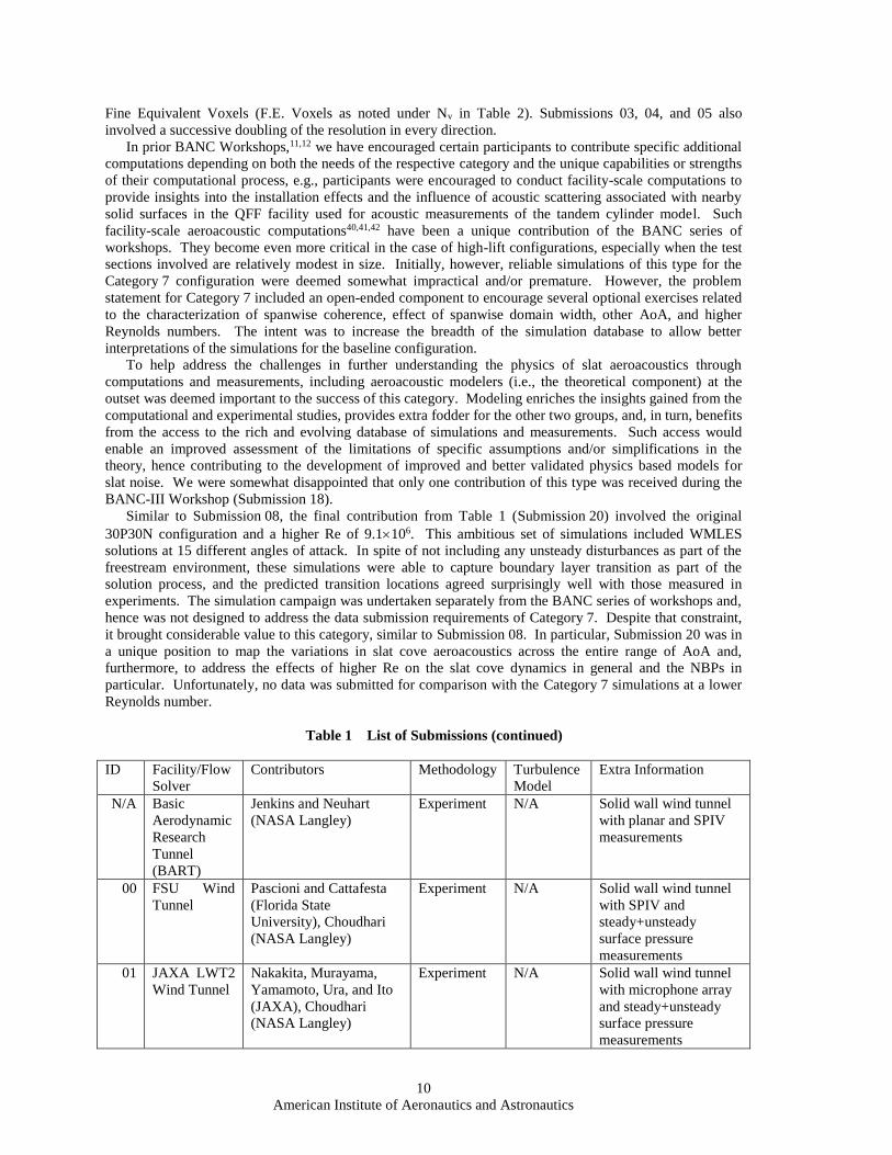
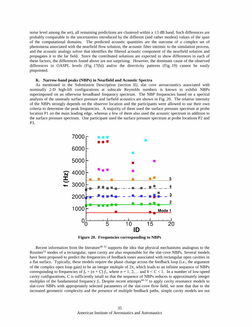
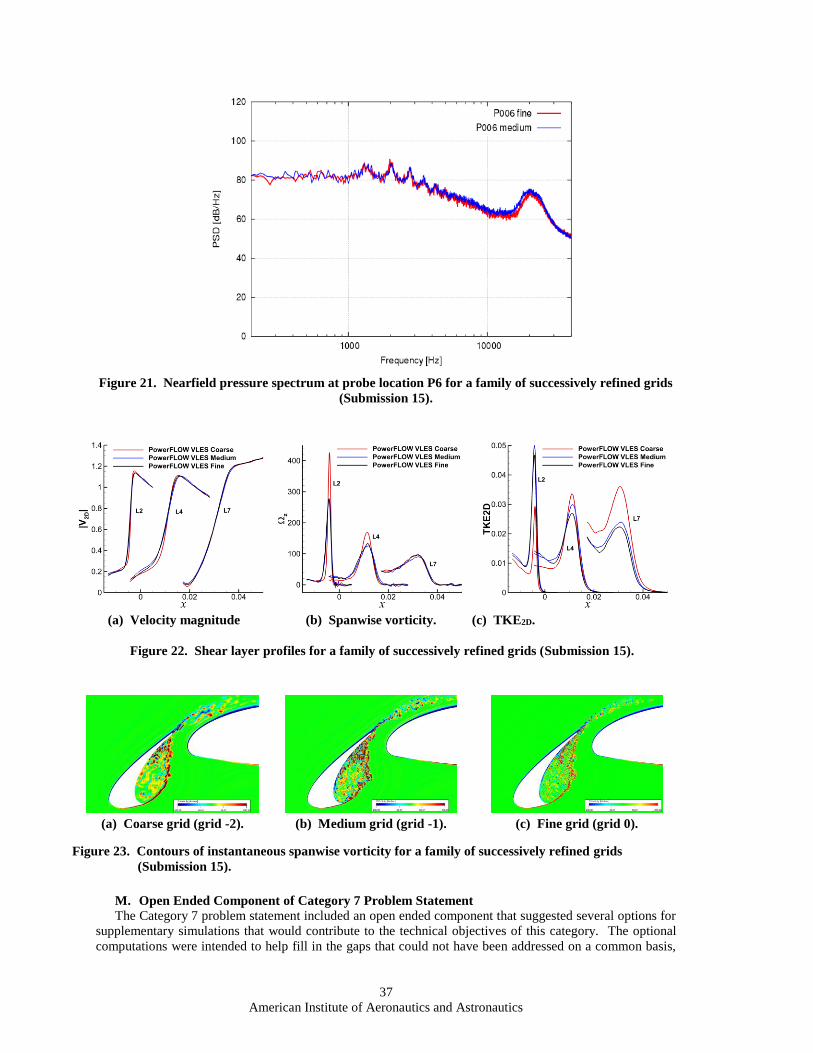
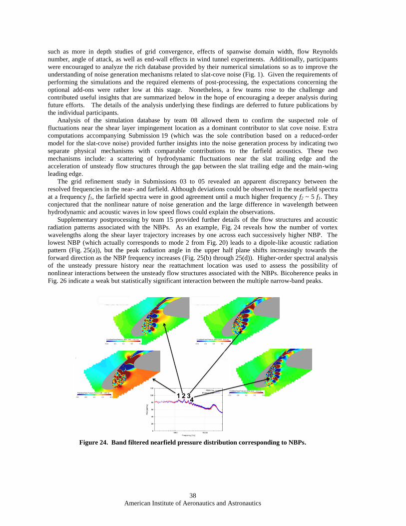
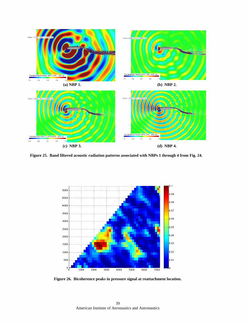
American Institute of Aeronautics and Astronautics 1 Assessment of Slat Noise Predictions for 30P30N High- Lift Configuration from BANC-III Workshop Meelan Choudhari 1 and David P. Lockard 2 NASA Langley Research Center, Hampton, VA 23681 and the BANC-III Category-7 Team 3 This paper presents a summary of the computational predictions and measurement data contributed to Category 7 of the 3 rd AIAA Workshop on Benchmark Problems for Airframe Noise Computations (BANC-III), which was held in Atlanta, GA, on June 14-15, 2014. Category 7 represents the first slat-noise configuration to be investigated under the BANC series of workshops, namely, the 30P30N two-dimensional high-lift model (with a slat contour that was slightly modified to enable unsteady pressure measurements) at an angle of attack that is relevant to approach conditions. Originally developed for a CFD challenge workshop to assess computational fluid dynamics techniques for steady high-lift predictions, the 30P30N configurations has provided a valuable opportunity for the airframe noise community to collectively assess and advance the computational and experimental techniques for slat noise. The contributed solutions are compared with each other as well as with the initial measurements that became available just prior to the BANC-III Workshop. Specific features of a number of computational solutions on the finer grids compare reasonably well with the initial measurements from FSU and JAXA facilities and/or with each other. However, no single solution (or a subset of solutions) could be identified as clearly superior to the remaining solutions. Grid sensitivity studies presented by multiple BANC-III participants demonstrated a relatively consistent trend of reduced surface pressure fluctuations, higher levels of turbulent kinetic energy in the flow, and lower levels of both narrow band peaks and the broadband component of unsteady pressure spectra in the nearfield and farfield. The lessons learned from the BANC-III contributions have been used to identify improvements to the problem statement for future Category-7 investigations. Nomenclature a = speed of sound bsim = spanwise extent of simulation domain b = model span c = chord length of stowed configuration = 0.4572 m (18 inches) cs = slat chord Cd = computed overall drag coefficient (scaled by planform area cbsim) CL = computed overall lift coefficient (scaled by planform area cbsim) CL, RMS = computed RMS lift coefficient (scaled by planform area cbsim) CL,s = contribution to overall lift coefficient (scaled by planform area cbsim) from slat CL,m = contribution to overall lift coefficient (scaled by planform area cbsim) from main wing CL,f = contribution to overall lift coefficient (scaled by planform area cbsim) from flap 1 Aerospace Technologist, Computational AeroSciences Branch, M.S. 128. Associate Fellow, AIAA. 2 Aerospace Technologist, Computational AeroSciences Branch, M.S. 128. Senior Member, AIAA. 3 Team members are listed in Table 1. https://ntrs.nasa.gov/search.jsp?R=20160006011 2020-04-24T17:47:11+00:00Z
Transcript
American Institute of Aeronautics and Astronautics
1
Assessment of Slat Noise Predictions for 30P30N High-
Lift Configuration from BANC-III Workshop
Meelan Choudhari1 and David P. Lockard2
NASA Langley Research Center, Hampton, VA 23681
and the BANC-III Category-7 Team3
This paper presents a summary of the computational predictions and
measurement data contributed to Category 7 of the 3rd AIAA Workshop on
Benchmark Problems for Airframe Noise Computations (BANC-III), which was held
in Atlanta, GA, on June 14-15, 2014. Category 7 represents the first slat-noise
configuration to be investigated under the BANC series of workshops, namely, the
30P30N two-dimensional high-lift model (with a slat contour that was slightly
modified to enable unsteady pressure measurements) at an angle of attack that is
relevant to approach conditions. Originally developed for a CFD challenge
workshop to assess computational fluid dynamics techniques for steady high-lift
predictions, the 30P30N configurations has provided a valuable opportunity for the
airframe noise community to collectively assess and advance the computational and
experimental techniques for slat noise. The contributed solutions are compared with
each other as well as with the initial measurements that became available just prior
to the BANC-III Workshop. Specific features of a number of computational
solutions on the finer grids compare reasonably well with the initial measurements
from FSU and JAXA facilities and/or with each other. However, no single solution
(or a subset of solutions) could be identified as clearly superior to the remaining
solutions. Grid sensitivity studies presented by multiple BANC-III participants
demonstrated a relatively consistent trend of reduced surface pressure fluctuations,
higher levels of turbulent kinetic energy in the flow, and lower levels of both narrow
band peaks and the broadband component of unsteady pressure spectra in the
nearfield and farfield. The lessons learned from the BANC-III contributions have
been used to identify improvements to the problem statement for future Category-7
investigations.
Nomenclature
a = speed of sound
bsim = spanwise extent of simulation domain
b = model span
c = chord length of stowed configuration = 0.4572 m (18 inches)
cs = slat chord
Cd = computed overall drag coefficient (scaled by planform area cbsim)
CL = computed overall lift coefficient (scaled by planform area cbsim)
CL, RMS = computed RMS lift coefficient (scaled by planform area cbsim)
CL,s = contribution to overall lift coefficient (scaled by planform area cbsim) from slat
CL,m = contribution to overall lift coefficient (scaled by planform area cbsim) from main wing
CL,f = contribution to overall lift coefficient (scaled by planform area cbsim) from flap
1 Aerospace Technologist, Computational AeroSciences Branch, M.S. 128. Associate Fellow, AIAA. 2 Aerospace Technologist, Computational AeroSciences Branch, M.S. 128. Senior Member, AIAA. 3 Team members are listed in Table 1.
American Institute of Aeronautics and Astronautics
13
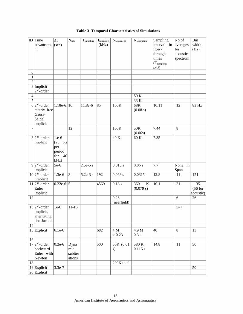
Table 3 Temporal Characteristics of Simulations
ID Time
advanceme
nt
t
(sec)
Nsub Tsampling fsampling
(kHz)
Nt,transient Nt,sampling Sampling
interval in
flow-
through
times
(Tsampling
c/U)
No of
averages
for
acoustic
spectrum
Bin
width
(Hz)
0
1
2
3 Implicit
2nd-order
4 50 K
5 33 K
6 2nd-order
matrix free
Gauss-
Seidel
implicit
1.18e-6 16 11.8e-6 85 100K 68K
(0.08 s)
10.11 12 83 Hz
7 12 100K 50K
(0.06s)
7.44 8
8 2nd-order
implicit
1.e-6
(25 pts
per
period
for 40
kHz)
40 K 60 K 7.35
9 2nd-order
implicit
5e-6 2.5e-5 s 0.015 s 0.06 s 7.7 None in
Span
10 2nd-order
implicit
1.3e-6 8 5.2e-3 s 192 0.069 s 0.0315 s 12.8 11 151
11 2nd-order
Euler
implicit
0.22e-6 5 4569 0.18 s 360 K
(0.079 s)
10.1 21 35
(56 for
acoustic)
12 0.23
(nearfield)
6 26
13 2nd-order
implicit,
alternating
line Jacobi
1e-6 11-16 5–7
14
15 Explicit 6.1e-6 682 4 M
> 0.23 s
4.9 M
0.3 s
40 8 13
16
17 2nd-order
backward
Euler with
Newton
0.2e-6 Dyna
mic
subiter
ations
500 50K (0.01
s)
580 K,
0.116 s
14.8 11 50
18 200K total
19 Explicit 3.3e-7 50
20 Explicit
American Institute of Aeronautics and Astronautics
14
Table 4 Computational Resources
* Perfect scaling assumed from the number of cores used in actual calculation to the reference number of
cores (i.e., 1,000)
ID CPU Hardware Interconnect Number
of cores
Wall clock time
per time step
(seconds)
Wall clock time for
1 sec simulation
with 1,000 cores*
(months)
0 N/A N/A N/A N/A N/A
1 N/A N/A N/A N/A N/A
2
3
4 SGI Altix ICE
Xeon(R) X5675 (Westmere),
3.07GHz
Infiniband®
QDR
228 86.9
3.5
5 1008 226
40.6
6 Xeon E5-2670 (8 cores) 256 1.5
7 64 0.3
8 SGI Altix 4700 240 16 s 1.5
9
10 HITACHI SR16000 32 23
11
12
13
14
15 SGI Altix ICE
Xeon(R) X5675 (Westmere),
3.07GHz
Infiniband®
QDR
3840 1.9
16 SGI Altix ICE
Xeon(R) X5675 (Westmere),
3.07GHz
Infiniband®
QDR
17 Nehalem nodes wth 2 quad-core
Intel Xeon X5560
Infiniband® 128 2 s 0.4
18 1 0.36 s 0.002
19 Intel Xeon E5420, 2.5 GHz 160 0.23
20 Sequoia supercomputer
American Institute of Aeronautics and Astronautics
15
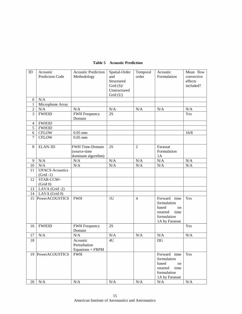
Table 5 Acoustic Prediction
ID Acoustic
Prediction Code
Acoustic Prediction
Methodology
Spatial-Order
and
Structured
Grid (S)/
Unstructured
Grid (U)
Temporal
order
Acoustic
Formulation
Mean flow
convective
effects
included?
0 N/A
1 Microphone Array
2 N/A N/A N/A N/A N/A N/A
3 FWH3D FWH Frequency
Domain
2S Yes
4 FWH3D
5 FWH3D
6 CFLOW 0.05 mm 16/8
7 CFLOW
0.05 mm
8 ELAN-3D FWH Time-Domain
(source-time
dominant algorithm)
2S 2 Farassat
Formulation
1A
9 N/A N/A N/A N/A N/A N/A
10 N/A N/A N/A N/A N/A N/A
11 UPACS-Acoustics
(Grid -1)
12 STAR-CCM+
(Grid 0)
13 LAVA (Grid -2)
14 LAVA (Grid 0)
15 PowerACOUSTICS
FWH 1U 4 Forward time
formulation
based on
retarted time
formulation
1A by Farassat
Yes
16 FWH3D
FWH Frequency
Domain
2S Yes
17 N/A N/A N/A N/A N/A N/A
18 Acoustic
Perturbation
Equations + FRPM
4U DG
19 PowerACOUSTICS FWH Forward time
formulation
based on
retarted time
formulation
1A by Farassat
Yes
20 N/A N/A N/A N/A N/A N/A
American Institute of Aeronautics and Astronautics
16
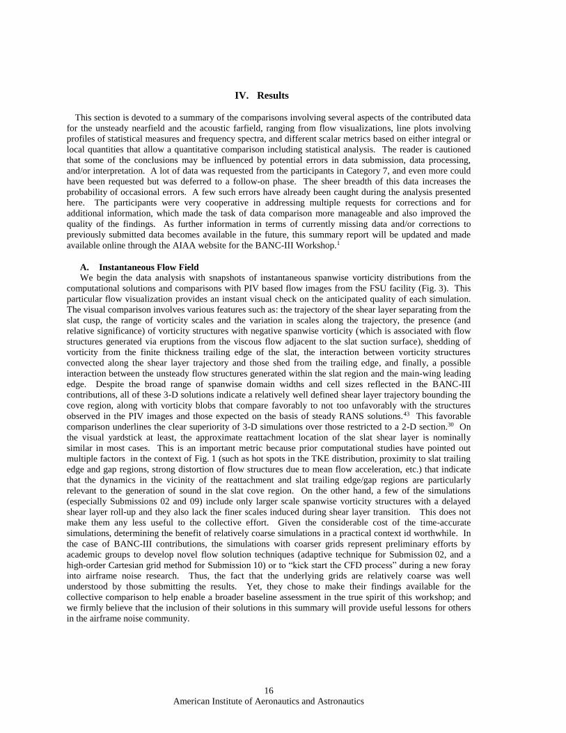
IV. Results
This section is devoted to a summary of the comparisons involving several aspects of the contributed data
for the unsteady nearfield and the acoustic farfield, ranging from flow visualizations, line plots involving
profiles of statistical measures and frequency spectra, and different scalar metrics based on either integral or
local quantities that allow a quantitative comparison including statistical analysis. The reader is cautioned
that some of the conclusions may be influenced by potential errors in data submission, data processing,
and/or interpretation. A lot of data was requested from the participants in Category 7, and even more could
have been requested but was deferred to a follow-on phase. The sheer breadth of this data increases the
probability of occasional errors. A few such errors have already been caught during the analysis presented
here. The participants were very cooperative in addressing multiple requests for corrections and for
additional information, which made the task of data comparison more manageable and also improved the
quality of the findings. As further information in terms of currently missing data and/or corrections to
previously submitted data becomes available in the future, this summary report will be updated and made
available online through the AIAA website for the BANC-III Workshop.1
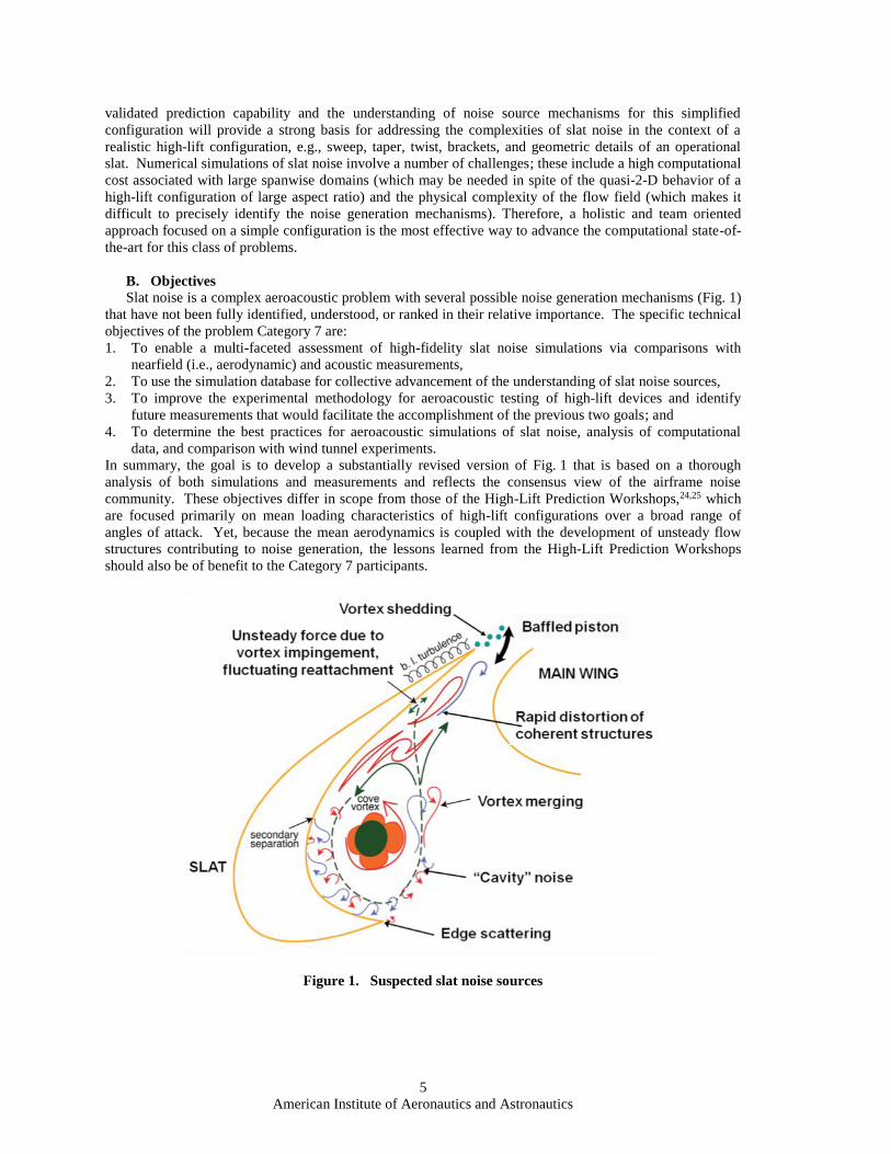
A. Instantaneous Flow Field
We begin the data analysis with snapshots of instantaneous spanwise vorticity distributions from the
computational solutions and comparisons with PIV based flow images from the FSU facility (Fig. 3). This
particular flow visualization provides an instant visual check on the anticipated quality of each simulation.
The visual comparison involves various features such as: the trajectory of the shear layer separating from the
slat cusp, the range of vorticity scales and the variation in scales along the trajectory, the presence (and
relative significance) of vorticity structures with negative spanwise vorticity (which is associated with flow
structures generated via eruptions from the viscous flow adjacent to the slat suction surface), shedding of
vorticity from the finite thickness trailing edge of the slat, the interaction between vorticity structures
convected along the shear layer trajectory and those shed from the trailing edge, and finally, a possible
interaction between the unsteady flow structures generated within the slat region and the main-wing leading
edge. Despite the broad range of spanwise domain widths and cell sizes reflected in the BANC-III
contributions, all of these 3-D solutions indicate a relatively well defined shear layer trajectory bounding the
cove region, along with vorticity blobs that compare favorably to not too unfavorably with the structures
observed in the PIV images and those expected on the basis of steady RANS solutions.43 This favorable
comparison underlines the clear superiority of 3-D simulations over those restricted to a 2-D section.30 On
the visual yardstick at least, the approximate reattachment location of the slat shear layer is nominally
similar in most cases. This is an important metric because prior computational studies have pointed out
multiple factors in the context of Fig. 1 (such as hot spots in the TKE distribution, proximity to slat trailing
edge and gap regions, strong distortion of flow structures due to mean flow acceleration, etc.) that indicate
that the dynamics in the vicinity of the reattachment and slat trailing edge/gap regions are particularly
relevant to the generation of sound in the slat cove region. On the other hand, a few of the simulations
(especially Submissions 02 and 09) include only larger scale spanwise vorticity structures with a delayed
shear layer roll-up and they also lack the finer scales induced during shear layer transition. This does not
make them any less useful to the collective effort. Given the considerable cost of the time-accurate
simulations, determining the benefit of relatively coarse simulations in a practical context id worthwhile. In
the case of BANC-III contributions, the simulations with coarser grids represent preliminary efforts by
academic groups to develop novel flow solution techniques (adaptive technique for Submission 02, and a
high-order Cartesian grid method for Submission 10) or to “kick start the CFD process” during a new foray
into airframe noise research. Thus, the fact that the underlying grids are relatively coarse was well
understood by those submitting the results. Yet, they chose to make their findings available for the
collective comparison to help enable a broader baseline assessment in the true spirit of this workshop; and
we firmly believe that the inclusion of their solutions in this summary will provide useful lessons for others
in the airframe noise community.
American Institute of Aeronautics and Astronautics
17
Figure 3. Visualization on instantaneous spanwise vorticity in xy plane.
(a) 00 (b) 02 (c) 03 (d) 04
(e) 05 (f ) 06 (g) 07 (h) 08
(i) 09 (j ) 10 (k) 11 (l) 12
(m) 13 (n) 14 (o) 15 (p) 16
(q) 17 (r) 19
F igu r e 1. A t im e ser i es sh ow n of m agn et i c fi eld t h at d o es n ot ch an ge b ecau se w e ar e u sin g t h e sam e fi gu r e each t im e.
1 of 1
American Inst itute of Aeronaut ics and Ast ronaut ics
American Institute of Aeronautics and Astronautics
18
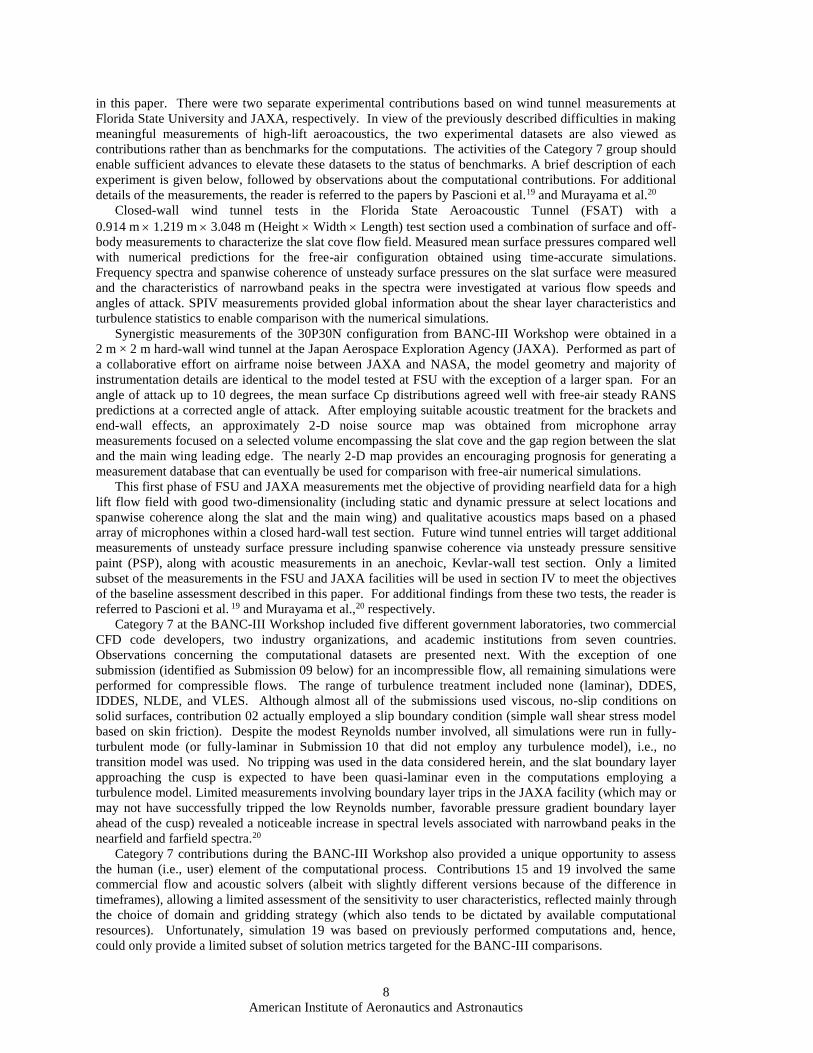
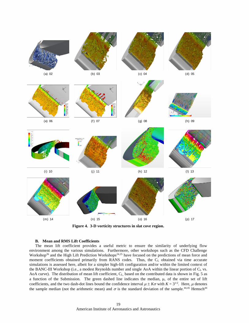
As noted in the previous paragraph, the flow structures in the slat cove region are intrinsically 3-D and
hence, a planar cross-section of the instantaneous flow field provides only limited insight into the overall
dynamics of the flow. To complement the spanwise vorticity contours in Fig. 3, the Category 7 participants
were also asked to provide a perspective view of an isosurface of instantaneous streamwise vorticity colored
by density (Fig. 4). These images illustrate the evolution of vorticity structures in the shear layer from
quasi-2-D Kelvin-Helmholtz rollers near the cusp to increasingly 3-D behavior farther downstream along the
shear layer trajectory. The emergence of streamwise elongated flow structures due to vorticity stretching
near the gap between the slat and the main wing may also be noted in many cases. The granularity of the
fine scale structures varies quite a bit, e.g., the images for Submissions 12, 14, 15, 17, and perhaps, 08 and
10 as well, indicate substantially finer structures than the remaining submissions. The range of scales
depends on both the grid resolution and the underlying CFD algorithm. The relatively broad range of scales
in Submission 10, despite the relatively coarse grid, may be related to the absence of any SGS or eddy
viscosity, together with a 4th-order discretization of the convective operator.
American Institute of Aeronautics and Astronautics
19
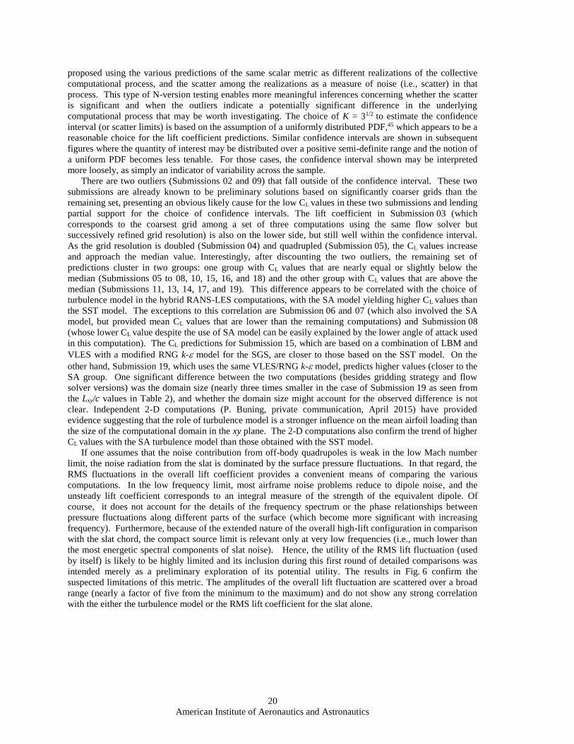
Figure 4. 3-D vorticity structures in slat cove region.
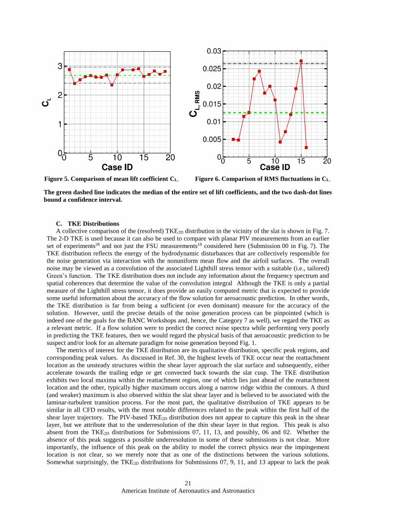
B. Mean and RMS Lift Coefficients
The mean lift coefficient provides a useful metric to ensure the similarity of underlying flow
environment among the various simulations. Furthermore, other workshops such as the CFD Challenge
Workshop26 and the High Lift Prediction Workshops24,25 have focused on the predictions of mean force and
moment coefficients obtained primarily from RANS codes. Thus, the CL obtained via time accurate
simulations is assessed here, albeit for a simpler high-lift configuration and/or within the limited context of
the BANC-III Workshop (i.e., a modest Reynolds number and single AoA within the linear portion of CL vs.
AoA curve). The distribution of mean lift coefficient, CL, based on the contributed data is shown in Fig. 5 as
a function of the Submission. The green dashed line indicates the median, of the entire set of lift
coefficients, and the two dash-dot lines bound the confidence interval K with K = 31/2. Here, denotes
the sample median (not the arithmetic mean) and is the standard deviation of the sample.44,45 Hemsch44
(a) 02 (b) 03 (c) 04 (d) 05
(e) 06 (f ) 07 (g) 08 (h) 09
(i) 10 (j ) 11 (k) 12 (l) 13
(m) 14 (n) 15 (o) 16 (p) 17
F igu r e 1. A t im e ser i es sh ow n of m agn et i c fi eld t h at d o es n ot ch an ge b ecau se w e ar e u sin g t h e sam e fi gu r e each t im e.
1 of 1
American Inst itute of Aeronaut ics and Ast ronaut ics
American Institute of Aeronautics and Astronautics
20
proposed using the various predictions of the same scalar metric as different realizations of the collective
computational process, and the scatter among the realizations as a measure of noise (i.e., scatter) in that
process. This type of N-version testing enables more meaningful inferences concerning whether the scatter
is significant and when the outliers indicate a potentially significant difference in the underlying
computational process that may be worth investigating. The choice of K = 31/2 to estimate the confidence
interval (or scatter limits) is based on the assumption of a uniformly distributed PDF,45 which appears to be a
reasonable choice for the lift coefficient predictions. Similar confidence intervals are shown in subsequent
figures where the quantity of interest may be distributed over a positive semi-definite range and the notion of
a uniform PDF becomes less tenable. For those cases, the confidence interval shown may be interpreted
more loosely, as simply an indicator of variability across the sample.
There are two outliers (Submissions 02 and 09) that fall outside of the confidence interval. These two
submissions are already known to be preliminary solutions based on significantly coarser grids than the
remaining set, presenting an obvious likely cause for the low CL values in these two submissions and lending
partial support for the choice of confidence intervals. The lift coefficient in Submission 03 (which
corresponds to the coarsest grid among a set of three computations using the same flow solver but
successively refined grid resolution) is also on the lower side, but still well within the confidence interval.
As the grid resolution is doubled (Submission 04) and quadrupled (Submission 05), the CL values increase
and approach the median value. Interestingly, after discounting the two outliers, the remaining set of
predictions cluster in two groups: one group with CL values that are nearly equal or slightly below the
median (Submissions 05 to 08, 10, 15, 16, and 18) and the other group with CL values that are above the
median (Submissions 11, 13, 14, 17, and 19). This difference appears to be correlated with the choice of
turbulence model in the hybrid RANS-LES computations, with the SA model yielding higher CL values than
the SST model. The exceptions to this correlation are Submission 06 and 07 (which also involved the SA
model, but provided mean CL values that are lower than the remaining computations) and Submission 08
(whose lower CL value despite the use of SA model can be easily explained by the lower angle of attack used
in this computation). The CL predictions for Submission 15, which are based on a combination of LBM and
VLES with a modified RNG k- model for the SGS, are closer to those based on the SST model. On the
other hand, Submission 19, which uses the same VLES/RNG k- model, predicts higher values (closer to the
SA group. One significant difference between the two computations (besides gridding strategy and flow
solver versions) was the domain size (nearly three times smaller in the case of Submission 19 as seen from
the Lxy/c values in Table 2), and whether the domain size might account for the observed difference is not
clear. Independent 2-D computations (P. Buning, private communication, April 2015) have provided
evidence suggesting that the role of turbulence model is a stronger influence on the mean airfoil loading than
the size of the computational domain in the xy plane. The 2-D computations also confirm the trend of higher
CL values with the SA turbulence model than those obtained with the SST model.
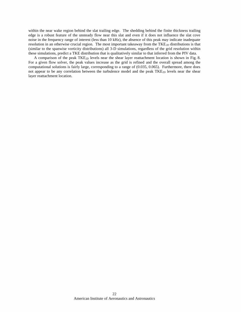
If one assumes that the noise contribution from off-body quadrupoles is weak in the low Mach number
limit, the noise radiation from the slat is dominated by the surface pressure fluctuations. In that regard, the
RMS fluctuations in the overall lift coefficient provides a convenient means of comparing the various
computations. In the low frequency limit, most airframe noise problems reduce to dipole noise, and the
unsteady lift coefficient corresponds to an integral measure of the strength of the equivalent dipole. Of
course, it does not account for the details of the frequency spectrum or the phase relationships between
pressure fluctuations along different parts of the surface (which become more significant with increasing
frequency). Furthermore, because of the extended nature of the overall high-lift configuration in comparison
with the slat chord, the compact source limit is relevant only at very low frequencies (i.e., much lower than
the most energetic spectral components of slat noise). Hence, the utility of the RMS lift fluctuation (used
by itself) is likely to be highly limited and its inclusion during this first round of detailed comparisons was
intended merely as a preliminary exploration of its potential utility. The results in Fig. 6 confirm the
suspected limitations of this metric. The amplitudes of the overall lift fluctuation are scattered over a broad
range (nearly a factor of five from the minimum to the maximum) and do not show any strong correlation
with the either the turbulence model or the RMS lift coefficient for the slat alone.
American Institute of Aeronautics and Astronautics
21
Figure 5. Comparison of mean lift coefficient CL. Figure 6. Comparison of RMS fluctuations in CL.
The green dashed line indicates the median of the entire set of lift coefficients, and the two dash-dot lines
bound a confidence interval.
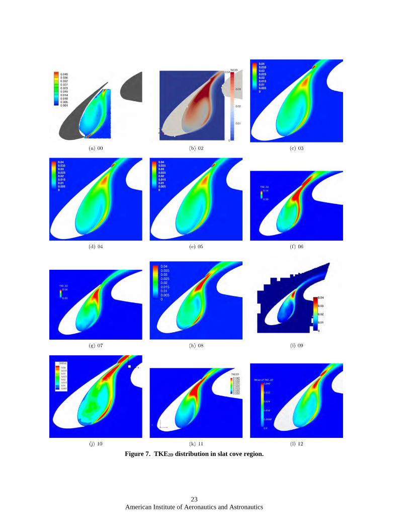
C. TKE Distributions
A collective comparison of the (resolved) TKE2D distribution in the vicinity of the slat is shown in Fig. 7.
The 2-D TKE is used because it can also be used to compare with planar PIV measurements from an earlier
set of experiments28 and not just the FSU measurements18 considered here (Submission 00 in Fig. 7). The
TKE distribution reflects the energy of the hydrodynamic disturbances that are collectively responsible for
the noise generation via interaction with the nonuniform mean flow and the airfoil surfaces. The overall
noise may be viewed as a convolution of the associated Lighthill stress tensor with a suitable (i.e., tailored)
Green’s function. The TKE distribution does not include any information about the frequency spectrum and
spatial coherences that determine the value of the convolution integral Although the TKE is only a partial
measure of the Lighthill stress tensor, it does provide an easily computed metric that is expected to provide
some useful information about the accuracy of the flow solution for aeroacoustic prediction. In other words,
the TKE distribution is far from being a sufficient (or even dominant) measure for the accuracy of the
solution. However, until the precise details of the noise generation process can be pinpointed (which is
indeed one of the goals for the BANC Workshops and, hence, the Category 7 as well), we regard the TKE as
a relevant metric. If a flow solution were to predict the correct noise spectra while performing very poorly
in predicting the TKE features, then we would regard the physical basis of that aeroacoustic prediction to be
suspect and/or look for an alternate paradigm for noise generation beyond Fig. 1.
The metrics of interest for the TKE distribution are its qualitative distribution, specific peak regions, and
corresponding peak values. As discussed in Ref. 30, the highest levels of TKE occur near the reattachment
location as the unsteady structures within the shear layer approach the slat surface and subsequently, either
accelerate towards the trailing edge or get convected back towards the slat cusp. The TKE distribution
exhibits two local maxima within the reattachment region, one of which lies just ahead of the reattachment
location and the other, typically higher maximum occurs along a narrow ridge within the contours. A third
(and weaker) maximum is also observed within the slat shear layer and is believed to be associated with the
laminar-turbulent transition process. For the most part, the qualitative distribution of TKE appears to be
similar in all CFD results, with the most notable differences related to the peak within the first half of the
shear layer trajectory. The PIV-based TKE2D distribution does not appear to capture this peak in the shear
layer, but we attribute that to the underresolution of the thin shear layer in that region. This peak is also
absent from the TKE2D distributions for Submissions 07, 11, 13, and possibly, 06 and 02. Whether the
absence of this peak suggests a possible underresolution in some of these submissions is not clear. More
importantly, the influence of this peak on the ability to model the correct physics near the impingement
location is not clear, so we merely note that as one of the distinctions between the various solutions.
Somewhat surprisingly, the TKE2D distributions for Submissions 07, 9, 11, and 13 appear to lack the peak
American Institute of Aeronautics and Astronautics
22
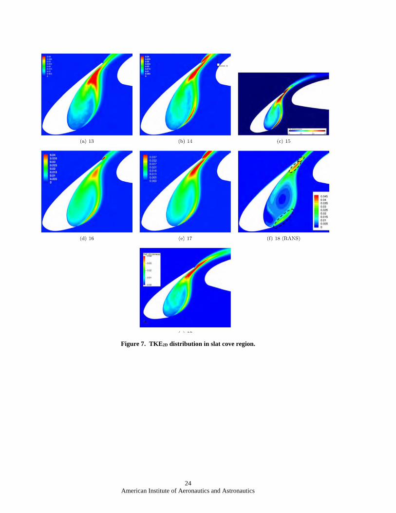
within the near wake region behind the slat trailing edge. The shedding behind the finite thickness trailing
edge is a robust feature of the unsteady flow near this slat and even if it does not influence the slat cove
noise in the frequency range of interest (less than 10 kHz), the absence of this peak may indicate inadequate
resolution in an otherwise crucial region. The most important takeaway from the TKE2D distributions is that
(similar to the spanwise vorticity distributions) all 3-D simulations, regardless of the grid resolution within
these simulations, predict a TKE distribution that is qualitatively similar to that inferred from the PIV data.
A comparison of the peak TKE2D levels near the shear layer reattachment location is shown in Fig. 8.
For a given flow solver, the peak values increase as the grid is refined and the overall spread among the
computational solutions is fairly large, corresponding to a range of (0.035, 0.065). Furthermore, there does
not appear to be any correlation between the turbulence model and the peak TKE2D levels near the shear
layer reattachment location.
American Institute of Aeronautics and Astronautics
23
Figure 7. TKE2D distribution in slat cove region.
American Institute of Aeronautics and Astronautics
24
Figure 7. TKE2D distribution in slat cove region.
American Institute of Aeronautics and Astronautics
25
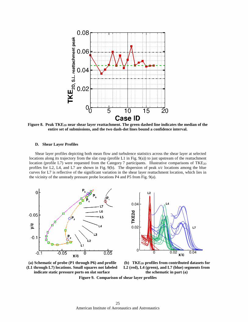
Figure 8. Peak TKE2D near shear layer reattachment. The green dashed line indicates the median of the
entire set of submissions, and the two dash-dot lines bound a confidence interval.
D. Shear Layer Profiles
Shear layer profiles depicting both mean flow and turbulence statistics across the shear layer at selected
locations along its trajectory from the slat cusp (profile L1 in Fig. 9(a)) to just upstream of the reattachment
location (profile L7) were requested from the Category 7 participants. Illustrative comparisons of TKE2D
profiles for L2, L4, and L7 are shown in Fig. 9(b). The dispersion of peak x/c locations among the blue
curves for L7 is reflective of the significant variation in the shear layer reattachment location, which lies in
the vicinity of the unsteady pressure probe locations P4 and P5 from Fig. 9(a).
(a) Schematic of probe (P1 through P6) and profile
(L1 through L7) locations. Small squares not labeled
indicate static pressure ports on slat surface
(b) TKE2D profiles from contributed datasets for
L2 (red), L4 (green), and L7 (blue) segments from
the schematic in part (a)
Figure 9. Comparison of shear layer profiles
American Institute of Aeronautics and Astronautics
26
E. Mean and RMS Surface Pressure Distribution
Consistent with the CL data in Fig. 5, the mean Cp distributions excluding the outliers are also indicative
of an analogous bimodal behavior. The two branches of the mean Cp distribution are plotted separately in
Figs. 10(a) and 10(b), respectively. The differences between the two branches are reflected in the respective
suction peaks over the main wing, the suction peaks and the locations of pressure plateau (i.e., apparent
separation locations) over the flap, and most significantly, in the pressure levels over a majority of the
suction surface of the slat. Of course, because of the inter-element coupling within the 3-element high-lift
configuration, neither one (nor a selected subset) of these differences can be identified as the cause behind
the remaining features. These correlated facets of the overall differences are potentially associated with the
differences in turbulence model (and, secondarily, other factors such as domain size, farfield boundary
condition, etc.)
(a) Submissions 03–08, 15, and 16 compared with the FSU measurement (open symbols denote the CFD
predictions, whereas filled black circles denote the measurement)
(b) Submissions 11–14 and 17 compared with the JAXA measurement (open symbols denote the CFD
predictions, whereas filled black squares denote the measurement).
Figure 10. Two branches of mean Cp distribution.
The reader may note that the experiments at both FSU19 and JAXA20 were performed in closed-wall
wind tunnels with significant end wall effects that make it difficult to determine an effective angle of attack
American Institute of Aeronautics and Astronautics
27
independently of comparison with open-air, 2-D (or short-span) CFD computations. During both sets of
measurements (which were obtained immediately before the BANC-III Workshop), the “equivalent” free-air
angle of attack for the high-lift configuration in these facilities was identified via comparisons with separate
CFD solutions that represent the two different lobes of the bimodal Cp distribution. Hence, the measured Cp
distributions agree well with the respective branch of the CFD solutions. Of course, this discrepancy can be
rectified in principle by using a common reference to determine the “equivalent” free-air angle of attack
during future measurements. The ability to reconcile such differences represents a positive aspect of the
long-term, ongoing interplay between the computations and experiments related to this category.
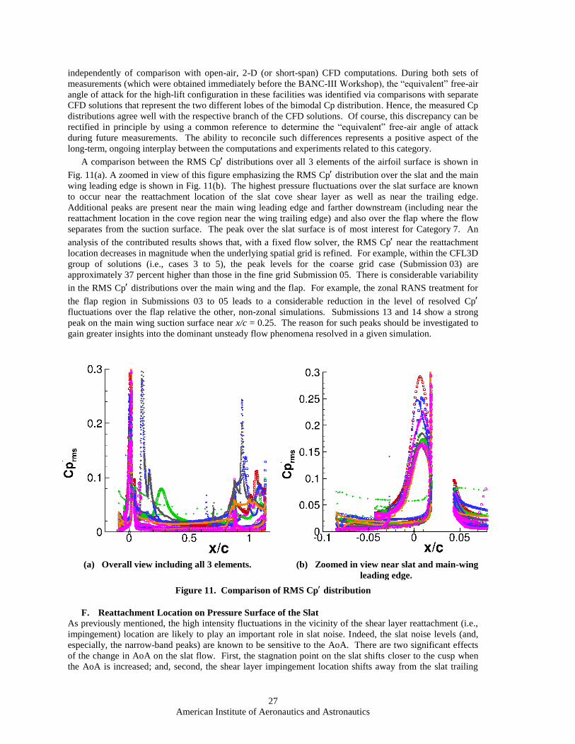
A comparison between the RMS Cp distributions over all 3 elements of the airfoil surface is shown in
Fig. 11(a). A zoomed in view of this figure emphasizing the RMS Cp distribution over the slat and the main
wing leading edge is shown in Fig. 11(b). The highest pressure fluctuations over the slat surface are known
to occur near the reattachment location of the slat cove shear layer as well as near the trailing edge.
Additional peaks are present near the main wing leading edge and farther downstream (including near the
reattachment location in the cove region near the wing trailing edge) and also over the flap where the flow
separates from the suction surface. The peak over the slat surface is of most interest for Category 7. An
analysis of the contributed results shows that, with a fixed flow solver, the RMS Cp near the reattachment
location decreases in magnitude when the underlying spatial grid is refined. For example, within the CFL3D
group of solutions (i.e., cases 3 to 5), the peak levels for the coarse grid case (Submission 03) are
approximately 37 percent higher than those in the fine grid Submission 05. There is considerable variability
in the RMS Cp distributions over the main wing and the flap. For example, the zonal RANS treatment for
the flap region in Submissions 03 to 05 leads to a considerable reduction in the level of resolved Cp fluctuations over the flap relative the other, non-zonal simulations. Submissions 13 and 14 show a strong
peak on the main wing suction surface near x/c = 0.25. The reason for such peaks should be investigated to
gain greater insights into the dominant unsteady flow phenomena resolved in a given simulation.
(a) Overall view including all 3 elements. (b) Zoomed in view near slat and main-wing
leading edge.
Figure 11. Comparison of RMS Cp distribution
F. Reattachment Location on Pressure Surface of the Slat
As previously mentioned, the high intensity fluctuations in the vicinity of the shear layer reattachment (i.e.,
impingement) location are likely to play an important role in slat noise. Indeed, the slat noise levels (and,
especially, the narrow-band peaks) are known to be sensitive to the AoA. There are two significant effects
of the change in AoA on the slat flow. First, the stagnation point on the slat shifts closer to the cusp when
the AoA is increased; and, second, the shear layer impingement location shifts away from the slat trailing
American Institute of Aeronautics and Astronautics
28
edge and the gap region. Both of these effects are likely to contribute to lower slat-noise levels observed at
higher AoA. Thus, a measure of the proximity between the source location (i.e., point of shear layer
impingement) and a potential catalyst underlying the partial conversion of hydrodynamic energy to acoustics
(i.e., slat trailing edge or the slat-main wing gap) is likely to be useful in interpreting the results. A
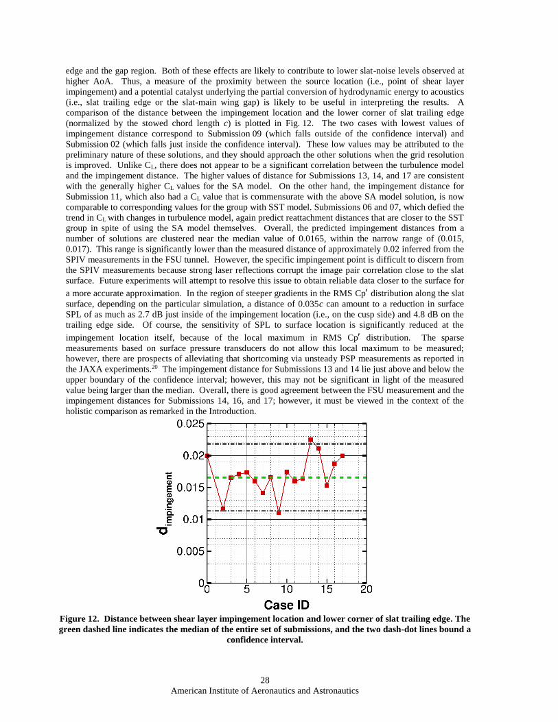
comparison of the distance between the impingement location and the lower corner of slat trailing edge
(normalized by the stowed chord length c) is plotted in Fig. 12. The two cases with lowest values of
impingement distance correspond to Submission 09 (which falls outside of the confidence interval) and
Submission 02 (which falls just inside the confidence interval). These low values may be attributed to the
preliminary nature of these solutions, and they should approach the other solutions when the grid resolution
is improved. Unlike CL, there does not appear to be a significant correlation between the turbulence model
and the impingement distance. The higher values of distance for Submissions 13, 14, and 17 are consistent
with the generally higher CL values for the SA model. On the other hand, the impingement distance for
Submission 11, which also had a CL value that is commensurate with the above SA model solution, is now
comparable to corresponding values for the group with SST model. Submissions 06 and 07, which defied the
trend in CL with changes in turbulence model, again predict reattachment distances that are closer to the SST
group in spite of using the SA model themselves. Overall, the predicted impingement distances from a
number of solutions are clustered near the median value of 0.0165, within the narrow range of (0.015,
0.017). This range is significantly lower than the measured distance of approximately 0.02 inferred from the
SPIV measurements in the FSU tunnel. However, the specific impingement point is difficult to discern from
the SPIV measurements because strong laser reflections corrupt the image pair correlation close to the slat
surface. Future experiments will attempt to resolve this issue to obtain reliable data closer to the surface for
a more accurate approximation. In the region of steeper gradients in the RMS Cp distribution along the slat
surface, depending on the particular simulation, a distance of 0.035c can amount to a reduction in surface
SPL of as much as 2.7 dB just inside of the impingement location (i.e., on the cusp side) and 4.8 dB on the
trailing edge side. Of course, the sensitivity of SPL to surface location is significantly reduced at the
impingement location itself, because of the local maximum in RMS Cp distribution. The sparse
measurements based on surface pressure transducers do not allow this local maximum to be measured;
however, there are prospects of alleviating that shortcoming via unsteady PSP measurements as reported in
the JAXA experiments.20 The impingement distance for Submissions 13 and 14 lie just above and below the
upper boundary of the confidence interval; however, this may not be significant in light of the measured
value being larger than the median. Overall, there is good agreement between the FSU measurement and the
impingement distances for Submissions 14, 16, and 17; however, it must be viewed in the context of the
holistic comparison as remarked in the Introduction.
Figure 12. Distance between shear layer impingement location and lower corner of slat trailing edge. The
green dashed line indicates the median of the entire set of submissions, and the two dash-dot lines bound a
confidence interval.
American Institute of Aeronautics and Astronautics
29
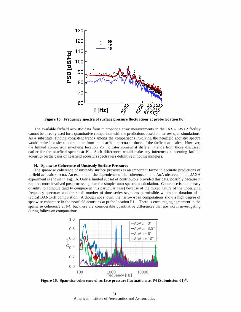
G. Unsteady Surface Pressure Spectra
Three different probe locations from the schematic in Fig. 8 are used to illustrate the comparison of
nearfield spectra based on surface pressure measurements. Figures 13 through 15 display the results for
probe locations P1, P4, and P6, respectively The probe location P4 is near the reattachment location of the
slat cove shear layer and, hence, is dominated by hydrodynamic fluctuations associated with the
impingement of the shear layer on the solid surface. The other two locations are not directly exposed to
hydrodynamic fluctuations and primarily represent the acoustic component of the unsteady surface pressure,
i.e., they may be viewed as representative (and easier to measure) metrics of the nearfield acoustics
associated with this configuration. Consequently, the spectral levels at P1 and P6 are more than 20 dB lower
than those at P4. The relatively intense broadband hydrodynamic fluctuations at P4 also tend to mask the
underlying narrowband peaks, which are more clearly observed in the frequency spectra at the P1 and P6
probe locations. The submission of data for the P6 probe location was optional. Hence, there were only
three entries that provided this spectrum and those are plotted in Fig. 15.
The P4 spectrum was measured in both the FSU and JAXA wind tunnels and, somewhat surprisingly,
exhibit an O(5) dB difference in their PSD amplitudes. Also, the NBPs in the FSU spectrum
(Submission 00) are better defined (i.e., sharper and attaining higher PSD values) than those in the JAXA
spectrum. The underlying shape of the broadband spectrum is quite similar across the full range of solutions,
including the (likely) underresolved Submission 02, which is unable to predict any NBPs and has PSD
values that are nearly 8–10 dB higher than even those in the JAXA measurement. The P4 spectrum based
on the finer of the two grids used for the simulations with the LAVA code matches the lower PSD values in
the FSU measurement pretty well up to approximately 2.2 kHz (i.e., past the second prominent NBP in the
portion of FSU spectrum included in this figure), but has levels at higher frequencies that are closer to those
of the P4 spectrum measured in the JAXA facility. The NBP frequencies are somewhat different from those
in the FSU spectrum as well. The spectra for Submissions 07 and 11 are somewhat similar up to and
including the second NBP and are not greatly different from the Submission 14 in this region, except for
rather intense NBPs in comparison with both the Submission 14 and both measured spectra. The
Submission 07 spectrum exhibits an earlier onset of rapid, high-frequency roll off, which could be an
indication of coarser grid resolution. The ostensibly underresolved simulation of Submission 09 appears to
have a reasonable broadband floor through 2.2 kHz, but has an overly strong NBP near 2 kHz and the
spectrum rolls off at lower frequencies than the spectrum for Submission 07. The spectrum for
Submission 12 compares favorably with the JAXA measurement through 3.5 kHz, but its slower roll-off
leads to higher PSD values at the higher frequencies. The Submission 15 spectrum falls roughly in between
the two measurements up to 4 kHz, i.e., over a major portion of the slat cove noise, but is closer to the JAXA
measurement for frequencies larger than 2.5 kHz. Of the three different grids used with the CFL3D solver,
the coarse grid spectrum (Submission 03) matches the JAXA measurement quite well through 4 kHz and
then rolls off rapidly. Improving the grid resolution delays the rolloff until f 7 kHz for Submission 04;
however, with an additional two-fold increase in the grid resolution (i.e., Submission 05), the PSD levels
become slightly smaller than the JAXA measurement up to 3 kHz, but they remain moderately above the
measurement from 4 kHz up to 10 kHz. Submission 06 yields a P4 spectrum that is relatively close to the
Submission 05 result and may actually be slightly closer to the JAXA measurement. Overall, the predicted
P4 spectra in Submissions 05, 08, 10, 15, 16, and 17 are similar to each other, with PSD variations of O(3)
dB or less.
To some degree, the aforementioned comparison is influenced by the differences in the probe location
relative the peak of RMS Cp distribution along the slat surface. Such differences can have a significant
impact on the measured PSD levels as mentioned in the preceding subsection in the course of comparing the
distance between the impingement location and the slat trailing edge. Again, global measurements
providing information about the RMS Cp levels and associated frequency spectra over a denser set of probe
locations would be useful in reconciling the discrepancy in PSD levels at probe location P4.
The comparison for the nearfield acoustic spectra at probe location P1 is somewhat similar to that
involving the primarily hydrodynamic spectra at probe location P4. Specifically, the spectral shapes are
again similar. Submission 02 shows PSD levels that are 10–20 dB higher than those in the JAXA
measurement up to 3 kHz, and the spectrum does not show any evidence of NBPs. The spectral shape for
Submission 12 is closer to that of the JAXA measurement across the entire range of frequencies, but the
American Institute of Aeronautics and Astronautics
30
levels are consistently 10–20 dB too high. A discrepancy of this magnitude in an otherwise well resolved
simulation would suggest a scaling error. However, that appears less likely since the spectrum plotted here
already corresponds to a revised submission after fixing a similar error. Submissions 09, 11, and 7 show
more intense peaks at NBP frequencies than the other predictions or the measurement. Predictions of
Submissions 03, 04, and 08 agree fairly well with each other and the measured spectrum, except for a
noticeable overprediction of PSD values at frequencies less than approximately 1.2 kHz. Submission 08
also shows stronger NBPs than the measured spectrum at frequencies beyond 3.5 kHz. The latter feature is
also shared by the P1 spectra in Submissions 05, 06, and 15, which have somewhat better agreement with
the measured spectrum at the lower frequencies (less than 1.2 kHz as noted above for Submissions 03, 04,
and 08) but also display a valley region (i.e., reduced PSDs) between approximately 2.8 kHz to 4 kHz. The
overall agreement between the JAXA measurement of the P1 spectrum and those predicted in Submissions
05, 06, and 15 is quite good, and possibly better than the agreement seen for probe location P4. Because the
P4 spectrum involves sound propagation from the slat cove region to the main wing leading edge, the
predicted spectra may be influenced by the narrow spanwise width of the domain, but perhaps not by much
in view of the relative proximity of those two regions. The spanwise width may play a greater role with
increasing distance from the slat cove region. The inclusion of more distant surface probe locations, such as
along the nose of the slat and/or on the pressure surface of the main wing, may be useful.
Figure 13. Frequency spectra of surface pressure
fluctuations at probe location P4.
Figure 14. Frequency spectra of surface pressure
fluctuations at probe location P1.
All three spectra for the P6 probe location agree well in shape. The predicted spectrum for
Submission 12 agrees with the measured spectrum in the FSU facility in both shape and the PSD levels,
except for the presence of an extra NBP near 1.6 kHz. The physical origin of the extra NBP is not clear at
this stage. On the other hand, the predicted spectrum for Submission 15 does not have the extra peak, but
the PSD values are 3–5 dB below the other two spectra. These differences may be, in part, due to the
sensitivity to probe location as discussed in the context of the P4 probe location. If so, choosing the P6
probe location in close proximity of the trailing edge may have been somewhat overambitious; and, in future
work, additional comparisons farther away from the trailing edge (in a flatter region of the RMS Cp distribution) may be more meaningful.
American Institute of Aeronautics and Astronautics
31
Figure 15. Frequency spectra of surface pressure fluctuations at probe location P6.
The available farfield acoustic data from microphone array measurements in the JAXA LWT2 facility
cannot be directly used for a quantitative comparison with the predictions based on narrow-span simulations.
As a substitute, finding consistent trends among the comparisons involving the nearfield acoustic spectra
would make it easier to extrapolate from the nearfield spectra to those of the farfield acoustics. However,
the limited comparison involving location P6 indicates somewhat different trends from those discussed
earlier for the nearfield spectra at P1. Such differences would make any inferences concerning farfield
acoustics on the basis of nearfield acoustics spectra less definitive if not meaningless.
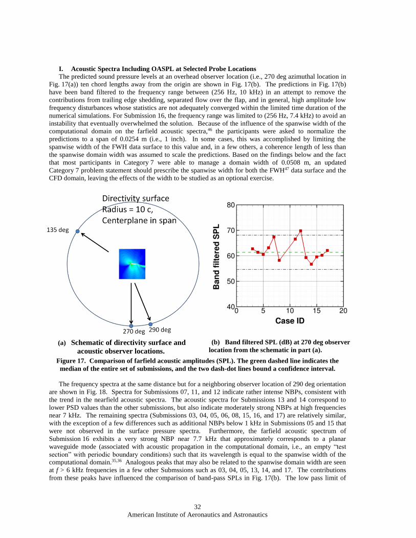
H. Spanwise Coherence of Unsteady Surface Pressures
The spanwise coherence of unsteady surface pressures is an important factor in accurate predictions of
farfield acoustic spectra. An example of the dependence of the coherence on the AoA observed in the JAXA
experiment is shown in Fig. 16. Only a limited subset of contributors provided this data, possibly because it
requires more involved postprocessing than the simpler auto-spectrum calculation. Coherence is not an easy
quantity to compute (and to compare in this particular case) because of the mixed nature of the underlying
frequency spectrum and the small number of time series segments permissible within the duration of a
typical BANC-III computation. Although not shown, the narrow-span computations show a high degree of
spanwise coherence in the nearfield acoustics at probe location P1. There is encouraging agreement in the
spanwise coherence at P4, but there are considerable quantitative differences that are worth investigating
during follow-on computations.
Figure 16. Spanwise coherence of surface pressure fluctuations at P4 (Submission 01)20.
0.0
0.2
0.4
0.6
0.8
1.0
100 1000 10000
Co
h2
Frequency [Hz]
AoAu = 0°AoAu = 3.5°AoAu = 6°AoAu = 10°
American Institute of Aeronautics and Astronautics
32
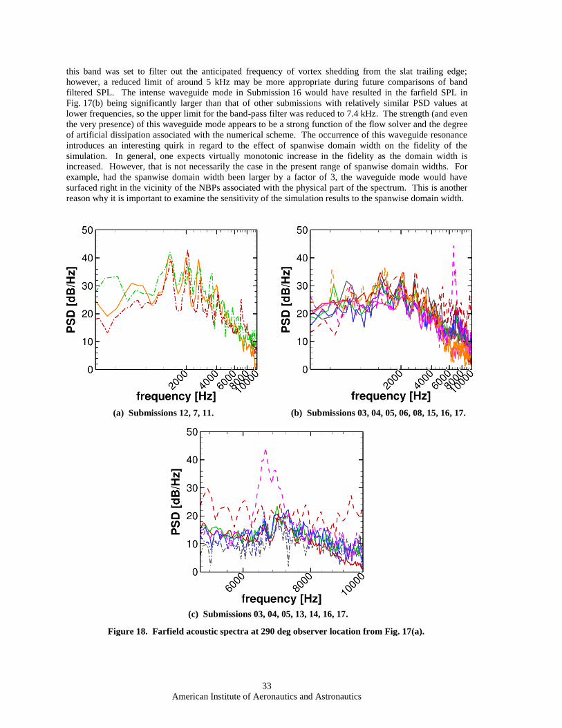
I. Acoustic Spectra Including OASPL at Selected Probe Locations
The predicted sound pressure levels at an overhead observer location (i.e., 270 deg azimuthal location in
Fig. 17(a)) ten chord lengths away from the origin are shown in Fig. 17(b). The predictions in Fig. 17(b)
have been band filtered to the frequency range between (256 Hz, 10 kHz) in an attempt to remove the
contributions from trailing edge shedding, separated flow over the flap, and in general, high amplitude low
frequency disturbances whose statistics are not adequately converged within the limited time duration of the
numerical simulations. For Submission 16, the frequency range was limited to (256 Hz, 7.4 kHz) to avoid an
instability that eventually overwhelmed the solution. Because of the influence of the spanwise width of the
computational domain on the farfield acoustic spectra,46 the participants were asked to normalize the
predictions to a span of 0.0254 m (i.e., 1 inch). In some cases, this was accomplished by limiting the
spanwise width of the FWH data surface to this value and, in a few others, a coherence length of less than
the spanwise domain width was assumed to scale the predictions. Based on the findings below and the fact
that most participants in Category 7 were able to manage a domain width of 0.0508 m, an updated
Category 7 problem statement should prescribe the spanwise width for both the FWH47 data surface and the
CFD domain, leaving the effects of the width to be studied as an optional exercise.
(a) Schematic of directivity surface and
acoustic observer locations.
(b) Band filtered SPL (dB) at 270 deg observer
location from the schematic in part (a).
Figure 17. Comparison of farfield acoustic amplitudes (SPL). The green dashed line indicates the
median of the entire set of submissions, and the two dash-dot lines bound a confidence interval.
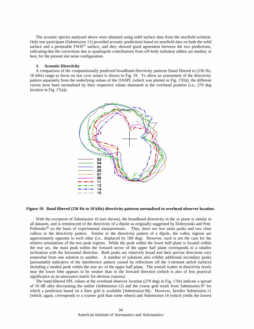
The frequency spectra at the same distance but for a neighboring observer location of 290 deg orientation
are shown in Fig. 18. Spectra for Submissions 07, 11, and 12 indicate rather intense NBPs, consistent with
the trend in the nearfield acoustic spectra. The acoustic spectra for Submissions 13 and 14 correspond to
lower PSD values than the other submissions, but also indicate moderately strong NBPs at high frequencies
near 7 kHz. The remaining spectra (Submissions 03, 04, 05, 06, 08, 15, 16, and 17) are relatively similar,
with the exception of a few differences such as additional NBPs below 1 kHz in Submissions 05 and 15 that
were not observed in the surface pressure spectra. Furthermore, the farfield acoustic spectrum of
Submission 16 exhibits a very strong NBP near 7.7 kHz that approximately corresponds to a planar
waveguide mode (associated with acoustic propagation in the computational domain, i.e., an empty “test
section” with periodic boundary conditions) such that its wavelength is equal to the spanwise width of the
computational domain.35,36 Analogous peaks that may also be related to the spanwise domain width are seen
at f > 6 kHz frequencies in a few other Submssions such as 03, 04, 05, 13, 14, and 17. The contributions
from these peaks have influenced the comparison of band-pass SPLs in Fig. 17(b). The low pass limit of
American Institute of Aeronautics and Astronautics
33
this band was set to filter out the anticipated frequency of vortex shedding from the slat trailing edge;
however, a reduced limit of around 5 kHz may be more appropriate during future comparisons of band
filtered SPL. The intense waveguide mode in Submission 16 would have resulted in the farfield SPL in
Fig. 17(b) being significantly larger than that of other submissions with relatively similar PSD values at
lower frequencies, so the upper limit for the band-pass filter was reduced to 7.4 kHz. The strength (and even
the very presence) of this waveguide mode appears to be a strong function of the flow solver and the degree
of artificial dissipation associated with the numerical scheme. The occurrence of this waveguide resonance
introduces an interesting quirk in regard to the effect of spanwise domain width on the fidelity of the
simulation. In general, one expects virtually monotonic increase in the fidelity as the domain width is
increased. However, that is not necessarily the case in the present range of spanwise domain widths. For
example, had the spanwise domain width been larger by a factor of 3, the waveguide mode would have
surfaced right in the vicinity of the NBPs associated with the physical part of the spectrum. This is another
reason why it is important to examine the sensitivity of the simulation results to the spanwise domain width.
detached eddy simulations (DDES)), and meshing techniques (structured grid with contiguous, patched, or
overset interfaces between adjacent blocks, Cartesian meshes coupled with immersed boundary techniques
or surface elements, and unstructured grids). One of the contributions was related to reduced-order
modeling based on a stochastic source model combined with CAA propagation. Modeling contributions of
this type signify a welcome addition to Category 7, and the initial contribution during BANC-III should spur
additional submissions of this type during the follow-on workshops.
This paper focused on a comparison of the computational predictions submitted by the BANC-III
participants. Some of the comparisons involved solution metrics that were common to both experiments and
simulations, whereas a few others were restricted to the computational datasets alone. Grid sensitivity
studies presented by multiple BANC-III participants demonstrated a relatively consistent trend of reduced
surface pressure fluctuations, higher levels of turbulent kinetic energy in the flow, and lower levels of both
narrow band peaks and the broadband component of unsteady pressure spectra in the nearfield and farfield.
The computational datasets also allowed a limited assessment of user to user differences in the context of a
fixed flow solver as well as of the effects of using different flow solvers with the same computational mesh.
Specific features of a number of computational solutions on the finer grids compared reasonably well
with the initial measurements from the FSU and JAXA facilities and/or with each other. However, no single
solution (or a subset of solutions) could be identified as clearly superior to the remaining solutions. The
differences with the measured data were to be expected in view of the challenges in slat-noise prediction
(particularly the mixed, tonal and broadband character of the acoustic spectra and the quasi-2-D geometry)
as well as in the measurement of slat noise, the practical limitations on the spanwise width of the
computational domain, and the finite end effects in both experiments from BANC-III.
The relatively consistent findings across the contributed set of computational solutions include a likely
effect of turbulence model on the mean lift and surface Cp distribution, an increase in TKE levels at higher
grid resolutions, and, yet, an accompanying decrease in the RMS surface pressure fluctuations and the
predicted farfield acoustic intensity. Grid resolutions had a particularly significant impact on the
narrowband peaks (NBPs) that became more intense at the coarse grid resolutions. For second-order CFD
discretizations and the typical span lengths used during the BANC-III contributions, an overall grid size of
10 million cells or less is not likely to yield acceptable predictions (at least in terms of allowing a fair
assessment of the underlying methodology and/or the overall computational process), although certain
features such as the NBP frequencies may be captured reasonably well in some of these cases.
The agreement for nearfield surface pressure spectra between the two facilities and also among the
various computations indicates larger differences than those previously seen for the similarly quasi-two-
dimensional tandem cylinder configuration used for Category 2 of the BANC-I and BANC-II workshops.
However, there is a good chance that the above difference will be narrowed by using a common (or, at least,
similar) set of grids as well as a prescribed spanwise domain during future studies.
The variations in NBP amplitudes appear to be greater than those in the broadband component of the
nearfield (i.e., surface pressure) and the farfield spectra. In contrast, the overall agreement between the
predicted NBP frequencies is rather encouraging. Even in experiments, the limited measurements acquired
at JAXA suggest that the NBP amplitudes are rather sensitive to boundary layer trips. These observations
lead us to conclude that limiting the comparison to the broadband component of noise spectra may provide
more robust comparisons, especially in the near term. The comparisons further indicate that the variability in
the nearfield acoustic spectra is less than that in the unsteady pressure spectra near the impingement
location. Therefore, additional comparisons related to the sensitivity of PSD levels to the probe location
near the reattachment would be helpful.
A few noteworthy accomplishments of the Category 7 at BANC-III are: assessment of slat noise
prediction using a broad set of methodologies, a promising start to investigating the sensitivity of the
American Institute of Aeronautics and Astronautics
41
computational predictions to numerical parameters including grid resolution, and a limited initial success
towards relatively grid-insensitive aeroacoustic predictions. On the experimental side, a useful start was
made to lay the foundation for a more comprehensive aeroacoustic dataset in the near future.
Integration between simulations and experiments has been a critical ingredient in facilitating the BANC
goal of enabling substantial collaborative advances in physics based predictions of airframe noise.
Category 7 has been consistent with the holistic focus on measurements targeted in the BANC workshops,
seeking an eventual characterization of the significant links between flow turbulence and the final metric of
interest in the form of farfield acoustics. The multi-faceted comparison will provide increased confidence
into the reliability of the simulation process as well as a better understanding of the physics of noise
generation, which is critical to the development of reduced-order prediction models for design cycle
applications as well as robust yet efficient noise reduction techniques. Furthermore, the simpler benchmarks
such as Category 7 will provide valuable lessons for the measurement and simulation of more complex
airframe noise configurations. Yet, several opportunities still remain to improve the computational and
experimental methodologies and those would be addressed during the future BANC workshops.
The contributions to the BANC-III Workshop have suggested several improvements for the follow-on
BANC-IV Workshop. To enable more meaningful comparisons, the computational grids developed for
BANC-III studies (along with additional grids derived from those) will be made available for future
Category 7 investigations, along with stricter guidelines concerning the spanwise domain width for nearfield
and farfield predictions. An additional, complementary test condition involving a larger angle of attack will
be included in the problem statement to allow an assessment specifically for the broadband component of
slat noise.
Unlike the previously investigated quasi-2-D configuration of tandem Cylinders, which was envisioned
as a prototype for the BANC effort and, hence, a comprehensive database was acquired prior to the
workshops, the Category 7 represents an effort to evolve a complex problem with group effort. As such, the
experimental efforts are evolving concurrently with the computational simulations, enabling a unique
platform for meaningful interactions between computations and measurements. A major focus of the future
measurements with the 30P30N configuration will include an improved set of acoustic measurements in a
Kevlar-wall wind tunnel and an improved strategy for processing the microphone array data for comparison
with acoustic predictions from narrow-span computations. The Kevlar-wall setup has the advantage of
reproducing an aerodynamic loading that is very close to that in a closed-wall test section and an acoustic
farfield that can still be measured without the major effects associated with acoustic reverberation in the
closed-wall test section. Additional measurements are planned that will provide unsteady PSP measurements
and, potentially, direct measurements of the state of the boundary layer near the slat cusp, providing a more
in-depth characterization of the effects of boundary layer tripping.
Despite the differences in computations and measurements noted in this paper, the overall set of
contributions to the BANC-III workshop indicate a positive prognosis for the BANC-IV Workshop,
provided that the model installation effects in the wind tunnel can be addressed satisfactorily. In closing, we
hope that this summary has provided a useful baseline to evaluate future progress and that it will be useful to
interested participants in building upon the existing contributions to this problem category (as well as the
related Category 6 under the BANC series of workshops54), and also to the broader airframe noise
community.
Acknowledgments
This work was performed as part of the Acoustics discipline under the Advanced Air Transportation
Technologies (AATT) project of NASA’s Fundamental Aeronautics Program. The authors would like to
acknowledge the contributions of all Category 7 participants in the BANC-III Workshop in Atlanta, GA,
during June 14-15, 2014. Particular thanks are due to the JAXA team (Drs. Murayama, Nakakita,
Yamamoto, Ura, and Ito) and the personnel at Florida State University (Mr. Pascioni and Prof. Cattafesta)
who performed the aerodynamic and/or aeroacoustic measurements of the 30P30N high-lift configuration.
Thanks are also due to various personnel at NASA Langley who supported the experiments in the BART
facility (Mr. Jenkins, Mr. Neuhart, Dr. Khorrami, Ms McGinely, Drs. Lin and Yao) and others (Mr. Weber,
Mr. Cagle, Mr. Hall, and members of the NASA Langley fabrication shop) who played an important role in
hardware design and fabrication of the instrumented slat model that was used for testing in the FSU facility.
The authors also acknowledge Dr. Pieter Buning for his assistance in enabling an assessment of domain-size
and turbulence-model effects on the mean lift coefficient. Finally, any success achieved by Category 7 of
American Institute of Aeronautics and Astronautics
42
the BANC-III Workshop is entirely due to the dedicated efforts of the various participants (listed in Table 1
of the paper) and all of them are acknowledged as honorary coauthors of this summary report. However, the
first author assumes all responsibility for the inferences drawn from the comparison presented herein as well
as for any errors in processing the data provided by the participants.
References 1 Third AIAA Workshop on Benchmark Problems for Airframe Noise Computations (BANC–III), URL:
https://info.aiaa.org/tac/ASG/FDTC/DG/BECAN_files_/BANCIII.htm [cited 15 April 2015]. 2 1st AIAA CFD Drag Prediction Workshop, Anaheim, CA, June 2001, URL:
http://aaac.larc.nasa.gov/tsab/cfdlarc/aiaa-dpw/Workshop1/workshop1.html [cited 15 April 2015]. 3 Levy, D. W., Vassberg, J. C., Wahls, R. A., Zickuhr, T., Agrawal, S., Pirzadeh, S., and Hemsch, M. J.,
“Summary of data from the first AIAA CFD Drag Prediction Workshop,” Journal of Aircraft, 40(5):875–882,
http://aaac.larc.nasa.gov/tsab/cfdlarc/aiaa-dpw/Workshop2/workshop2.html [cited 15 April 2015]. 5 Laflin, K. R., Vassberg, J. C., Wahls, R. A., Morrison, J. H., Brodersen, O., Rakowitz, M., Tinoco, E. N., and
Godard, J., “Summary of Data from the Second AIAA CFD Drag Prediction Workshop,” Journal of Aircraft,
Vol. 42, No. 5, pp. 1165–1178, 2005. 6 3rd AIAA CFD Drag Prediction Workshop, San Francisco, CA, June 2006, URL:
http://aaac.larc.nasa.gov/tsab/cfdlarc/aiaa-dpw/Workshop3/workshop3.html [cited 15 April 2015]. 7 Vassberg, J. C., Tinoco, E. N., Mani, M., Brodersen, O. P., Eisfeld, B., Wahls, R. A., Morrison, J. H., Zickuhr,
T., Laflin, K. R., and Mavriplis, D. J., “Abridged Summary of the Third AIAA CFD Drag Prediction
Workshop,” Journal of Aircraft, Vol. 45, No. 3, pp. 781–798, May–June 2008. 8 4th AIAA CFD Drag Prediction Workshop, San Antonio, TX, June 2009, URL:
http://aaac.larc.nasa.gov/tsab/cfdlarc/aiaa-dpw/Workshop4/workshop4.html, [cited 15 April 2015]. 9 Vassberg, J., Tinoco, E., Mani, M., Rider, B., Zickuhr, T., Levy, D., Broderson, O., Eisfeld, B., Crippa, S.,
Wahls, R., Morrison, J., Mavriplis, D., Murayama, M., “Summary of the Fourth AIAA CFD Drag Prediction
Workshop,” AIAA Paper 2010-4547, 2010. 10 Choudhari, M. and Yamamoto, K., “Integrating CFD, CAA, and Experiments towards Benchmark Datasets for
Airframe Noise Problems,” Proceedings of 5th Symposium on Integration CFD and Experiments in
Aerodynamics (Integration 2012), October 2012. 11 Proceedings of the First AIAA Workshop on Benchmark Problems for Airframe Noise Computations (BANC-
I), Stockholm, Sweden, June 2010. 12 Proceedings of the Second AIAA Workshop on Benchmark Problems for Airframe Noise Computations
(BANC-II), Colorado Springs, CO, June 2012. 13 Herr, M. and Kamruzzaman, M., “Benchmarking of Trailing-Edge Noise Computations|Outcome of the BANC-
II Workshop,” AIAA-Paper 2013-2123, May 2013. 14 Lockard. D.P., “Summary of the Tandem Cylinder Solutions from the Benchmark problems for Airframe Noise
Computations-I Workshop,” AIAAPaper 2011-353, 2011. 15 Spalart, P. R. and Mejia, K. M., “Analysis of Experimental and Numerical Studies of the Rudimentary Landing
Gear, AIAA Paper 2011-355, 2011. 16 Spalart, P. R. and Wetzel, D., “Rudimentary Landing Gear Results at the 2012 BANC-II Airframe Noise
Workshop,” Int. J. Aeroacoustics, Nos.1-2, Vol. 14, 2015, pp. 193–216. 17 NASA Slat Noise Configuration, URL:
https://info.aiaa.org/tac/ASG/FDTC/DG/BECAN_files_/BANCII_category 7, [cited 15 April 2015]. 18 Pascioni, K., Cattafesta, L. N., and Choudhari, M. M., “An Experimental Investigation of the 30P30N Multi-
Element High-Lift Airfoil,” AIAA Paper 2014-3062, 2014. 19 Murayama, M., Nakakita, K., Yamamoto, K., Ura, H., Ito, Y., and Choudhari, M. M., “Experimental Study on
Slat Noise from 30P30N hree-Element High-Lift Airfoil at JAXA Hard-Wall Lowspeed Wind Tunnel,” AIAA
Paper 2014-2080, 2014. 20 Khorrami, M. R. and Van de Ven, T., “Summary of Contributions to PDCC-NLG Category of BANC-II
Workshop,” Proceedings of AIAA BANC-II Workshop, Colorado Springs, CO, June 2012. 21 Manoha, E. and Caruelle, B., “Summary of the LAGOON Solutions from the Benchmark Problems for
Airframe Noise Computations-III Workshop,” To be presented at the 21st AIAA/CEAS Aeroacoustics
Conference, Dallas, TX, June 2015. 22 Lopes, L., Redonnet, S., Imamura, T., Ikeda, T., Zawodnyi, N., and Cunha, “Variability in the Propagation
Phase of CFD-Based Noise Prediction: Summary of Results from Category 8 of the BANC-III Workshop,” To
be presented at the 21st AIAA/CEAS Aeroacoustics Conference, Dallas, TX, June 2015. 23 Dobrzynski, W., “Almost 40 Years of Airframe Noise Research: What Did We Achieve?,” Journal of Aircraft,
American Institute of Aeronautics and Astronautics
43
24 Slotnick, J. P., Hannon, J. A., and Chaffin, M., “Overview of the First AIAA CFD High Lift Prediction
Workshop (Invited),” AIAA Paper 2011-862, January 2011. 25 Rumsey, C. L., Slotnick, J. P., Long, M., Stuever, R. A., and Wayman, T. R., “Summary of the First AIAA
CFD High-Lift Prediction Workshop,” Journal of Aircraft, Vol. 48, No. 6, 2011, pp. 2068–2079. 26 Klausmeyer, S. M., Lin, J. C., Comparative Results From a CFD Challenge Over a 2D Three-Element High-Lift
Airfoil," NASA TM 112858, May 1997. 27 Paschal, K., Jenkins, L., and Yao, C., “Unsteady Slat-Wake Characteristics of a High-Lift
Configuration,” AIAA Paper 2000-0139, January 2000. 28 Jenkins, L. N., Khorrami, M. R., and Choudhari, M. M., “Characterization of Unsteady Flow Structures Near
Leading-Edge Slat: Part I. PIV Measurements,” AIAA Paper 2004-2801, 2004. 29 Khorrami, M. R., Choudhari, M. M., and Jenkins, L. N., “Characterization of Unsteady Flow Structures Near
Leading-Edge Slat: Part II. 2-D Computations,” AIAA Paper 2004-2802, 2004. 30 Choudhari, M. and Khorrami, M. R., “Effect of Three-Dimensional Shear-Layer Structures on Slat Cove
Unsteadiness,” AIAA J., Vol. 45, No. 9, 2007, pp. 2174–2186,. 31 Lockard, D. P. and Choudhari, M., “Noise Radiation from a Leading-Edge Slat,” AIAA Paper 2009-3101, 2009. 32 Lockard, D. P. and Choudhari, M., “The Effect of Cross Flow on Slat Noise,” AIAA Paper 2010-3835, 2010. 33 Lockard, D. P. and Choudhari, M., “Variation of Slat Noise with Mach and Reynolds Numbers,” AIAA Paper
2011-2910, 2011. 34 Choudhari, M. M., Lockard, D. P., Khorrami, M. R., and Mineck, R. E., “Slat Noise Simulations: Status and
Challenges,” Proceedings of Inter-Noise 2011, ed. Hiroyuki Imaizumi, Osaka, Japan, Sept. 4-7, 2011. 35 Lockard, D. P., Choudhari, M. M., and Buning, P. G., “Grid Sensitivity Study for Slat Noise Simulations,”
AIAA Paper 2014-2627, 2014. 36 Lockard, D. P., Choudhari, M. M., and Buning, P. G., “Influence of Spanwise Boundary Conditions on Slat
Noise Simulations,” To be presented at the 21st AIAA/CEAS Aeroacoustics Conference, Dallas, TX, June
2015. 37 Third International Workshop on High-Order CFD Methods (C3.1 Turbulent flow over a multi-element airfoil),
Kissimmee, Florida, January 3-4, 2015, URL: https://www.grc.nasa.gov/hiocfd/ [cited 15 April 2015]. 38 C3.1 Turbulent flow over a multi-element airfoil (1/30/2011), [email protected],
URL: https://www.grc.nasa.gov/hiocfd/wp-content/uploads/sites/22/case_c3.1.pdf [cited 15 April 2015]. 39 Rumsey, C., Lee-Rausch, E., and Watson, R., “Three-dimensional effects in multi-element high lift
computations,” Computers and Fluids, Vol. 32, No. 5, 2003, pp. 631–657. 40 Bres, G., Freed, D., Wessels, M., Noelting, S., and Perot, F., “Flow and Noise Predictions for the Tandem
Cylinder Aeroacoustic Benchmark,” Phys. Fluids, Vol. 24, 036101, 2012; doi: 10.1063/1.3685102. 41 Tinetti, A. F. and Dunn, M. H. , “Acoustic Simulations of an Installed Tandem Cylinder Configuration,” AIAA
Paper 2009-3158, 2009. 42 Redonnet, S., Lockard, D.P., Khorrami, M.R., and Choudhari, M., “CFD-CAA Coupled Calculations of a
Tandem Cylinder Configuration to Assess Facility Installation Effects,” AIAA Paper 2011-2841, 2011. 43 Choudhari, M., Khorrami, M.R., Lockard, D.P., Atkins, H., and Lilley, G., “Slat Cove Noise Modeling: A
Posteriori Analysis of Unsteady RANS Simulations,” AIAA Paper 2002-2468, 2002. 44 Hemsch, M. J., “Statistical Analysis of CFD Solutions from the Drag Prediction Workshop,” J. Aircraft, Vol.
41, No. 1, 2004, pp. 95–103. 45 Morrison, J. H., “Statistical Analysis of CFD Solutions from the Fourth AIAA Drag Prediction Workshop,”
AIAA Paper 2010-4673, 2010. 46 Seo, J. H., Chang, K. W., and Moon, Y. J., “Aerodynamic Noise Prediction for Long-Span Bodies,” AIAA
Paper 2006-2573, 2006. 47 FfowcsWilliams, J. E. and Hawkings, D. L., “Sound Generation by Turbulence and Surfaces in Arbitrary
Motion,” Philosophical Transactions of the Royal Society, Vol. A264, No. 1151, 1969, pp. 321–342. 48 Dobrzynski, W. and Pott-Pollenske, M., “Slat Noise Source Studies for Farfield Noise Prediction,” AIAA Paper
2001-2158, 2001. 49 Roger, M. and Perennes, S., “Low-Frequency Noise Sources in Two-Dimensional High-Lift Devices,” AIAA
Paper 2000–1972, 2000. 50 Pott-Pollenske, M., Alvarez-Gonzalez, J., and Dobrzynski, W., “Effect of Slat Gap/Overlap on Farfield
Radiated Noise,” AIAA Paper 2003–3228, 2003. 51 Terracol, M., Manoha, E., and Lemoine, E., “Investigation of the Unsteady Flow and Noise Sources Generation
in a Slat Cove: Hybrid Zonal RANS/LES Simulation and Dedicated Experiment,” AIAA Paper 2011-3203,
2011. 52 Deck, S. and Laraufie, R., “Numerical Investigation of the Flow Dynamics Past a Three-element Aerofoil,”
Journal of Fluid Mechanics, Vol. 732, 2013, pp. 401–444. 53 Rossiter, J., “Wind-Tunnel Experiments on the Flow over Rectangular Cavities at Subsonic and Transonic
Speeds,” Aeronautical Research Council Reports and Memoranda 3438, 1966. 54 LEISA slat-noise configuration
URL: https://info.aiaa.org/tac/ASG/FDTC/DG/BECAN_files_/BANCII_category6 [cited 15 April 2015].