Assessment of the environmental impacts and sediment remediation potential associated with copper contamination from antifouling paint (and associated recommendations for management)

Catriona Macleod, Ruth Eriksen, Stuart Simpson,

Adam Davey and Jeff Ross

28th May 2014

FRDC Project No 2011-041

i

© 2014 Fisheries Research and Development Corporation. All rights reserved.

ISBN 978-1-86295-741-1

Assessment of the environmental impacts and sediment remediation potential associated with copper contamination from antifouling paint (and associated recommendations for management) FRDC Project 2011-041

2014

Ownership of Intellectual property rights Unless otherwise noted, copyright (and any other intellectual property rights, if any) in this publication is owned by the Fisheries Research and Development Corporation, University of Tasmania, and CSIRO.

This publication (and any information sourced from it) should be attributed to:

Macleod, C.M, Eriksen, R.S, Simpson, S.L, Davey, A. and Ross, J (2014) Assessment of the environmental impacts and sediment remediation potential associated with copper contamination from antifouling paint (and associated recommendations for management), FRDC Project 2011-041 (University of Tasmania, CSIRO), Australia.

Creative Commons licence All material in this publication is licensed under a Creative Commons Attribution 3.0 Australia Licence, save for content supplied by third parties, logos and the Commonwealth Coat of Arms.

Creative Commons Attribution 3.0 Australia Licence is a standard form licence agreement that allows you to copy, distribute, transmit and adapt this publication provided you attribute the work. A summary of the licence terms is available from creativecommons.org/licenses/by/3.0/au/deed.en. The full licence terms are available from creativecommons.org/licenses/by/3.0/au/legalcode.

Inquiries regarding the licence and any use of this document should be sent to: frdc@frdc.gov.au.

Disclaimer The authors do not warrant that the information in this document is free from errors or omissions. The authors do not accept any form of liability, be it contractual, tortious, or otherwise, for the contents of this document or for any consequences arising from its use or any reliance placed upon it. The information, opinions and advice contained in this document may not relate, or be relevant, to a readers particular circumstances. Opinions expressed by the authors are the individual opinions expressed by those persons and are not necessarily those of the publisher, research provider or the FRDC.

The Fisheries Research and Development Corporation plans, invests in and manages fisheries research and development throughout Australia. It is a statutory authority within the portfolio of the federal Minister for Agriculture, Fisheries and Forestry, jointly funded by the Australian Government and the fishing industry.

Researcher Contact Details FRDC Contact Details Name:

Address:

Phone:

Fax:

Email:

Catriona Macleod

IMAS, Taroona Laboratories

Nubeena Crescent Taroona TAS 7005

03 62 277 277

03 62 278 035

Catriona.Macleod@utas.edu.au

Address:

Phone:

Fax:

Email: Web:

25 Geils Court

Deakin ACT 2600

02 6285 0400

02 6285 0499

frdc@frdc.com.au

www.frdc.com.au

In submitting this report, the researcher has agreed to FRDC publishing this material in its edited form.

ii

Contents

List of Tables ........................................................................................................................................ iv

List of Figures ........................................................................................................................................ v

Acknowledgments .............................................................................................................................. viii

Abbreviations ...................................................................................................................................... viii

Executive Summary .............................................................................................................................. x

1 Introduction ..................................................................................................................................... 1

1.1. Background...........................................................................................................................1

1.2. Need ......................................................................................................................................1

1.3. Objectives .............................................................................................................................2

1.4. Study Design and Rationale .................................................................................................3

1.4.1 Ecotoxicology, Bioavailability & Associated Management Guidelines (Objective 1) ................................................................................................................................3

1.4.2 Recovery Potential and Associated Management Guidelines (Objective 2/ 3) ...........7

1.4.3 Broadscale Influences and Associated Management Guidelines (Objective 2/ 3) .....8

2 Methods.......................................................................................................................................... 10

2.1. Toxicity Assessments .........................................................................................................10

2.2. Assessment of Recovery Potential .....................................................................................10

2.2.1 Farm management regimes .........................................................................................11

2.2.2 Farm selection ............................................................................................................11

2.2.3 Metals .........................................................................................................................13

2.2.4 Bulk sediment properties ............................................................................................13

2.2.5 Porewaters ..................................................................................................................13

2.2.6 CTD profiles ...............................................................................................................16

2.2.7 Mesocosm sampling ...................................................................................................16

2.2.8 Site water ....................................................................................................................16

2.2.9 Particle size ................................................................................................................16

2.2.10 Total Organic Carbon and moisture content ..............................................................16

2.2.11 Acid volatile sulfide ...................................................................................................16

2.2.12 Oxygen Penetration Depth .........................................................................................17

2.2.13 Mesocosm incubations (nutrient processes) ...............................................................17

2.2.14 Macrofauna .................................................................................................................18

2.2.15 Long cores ..................................................................................................................18

2.2.16 Statistical analysis ......................................................................................................18

2.3. Broadscale assessment .......................................................................................................19

2.3.1 Sediment Traps ...........................................................................................................19

2.3.2 Site Selection / sampling design .................................................................................19

2.3.3 Exposure metrics ........................................................................................................21

2.3.4 Statistical analysis ......................................................................................................21

2.3.5 ADCP .........................................................................................................................22

3 Results and Discussion ................................................................................................................. 23

3.1. Ecotoxicology, bioavailability & associated management guidelines (Objective 1) .........23

iii

3.1.1 Paint behaviour, toxicity and bioavailability..............................................................23

3.1.2 Deriving management guidelines from toxicity data .................................................24

3.1.3 Thresholds derived from chronic effects data ............................................................24

3.1.4 Metal contaminant mixtures .......................................................................................25

3.1.5 Management limits for sediments contaminated by copper-based paint ...................29

3.1.6 Co-occurring zinc contamination ...............................................................................30

3.2. Recovery Potential & Associated Management Guidelines (Objective 2/ 3) ....................30

3.2.1 Short-term changes .....................................................................................................30

3.2.2 Long-term changes .....................................................................................................44

3.3. Broadscale Influences & Associated Management Guidelines (Objective 2/ 3) ...............49

3.3.1 Assessing background concentrations and the environmental factors that influence copper concentrations ................................................................................................49

3.3.2 Does farming practice influence background copper concentrations?.......................56

3.3.3 How do natural processes influence copper distribution within farms ......................61

3.3.4 Combining this information to Improve Management and Understanding ................62

4 General Conclusions ..................................................................................................................... 64

4.1. Toxicity – Biological Significance .....................................................................................64

4.2. Sediment Biogeochemistry .................................................................................................65

4.3. Management Recommendations ........................................................................................66

5 Implications ................................................................................................................................... 67

6 Recommendations ......................................................................................................................... 68

6.1. Further development ...........................................................................................................68

7 Extension and Adoption ............................................................................................................... 69

7.1. Project Coverage ................................................................................................................69

8 Project materials developed ......................................................................................................... 70

9 Appendices ..................................................................................................................................... 71

9.1. Appendix 1: List of researchers and project staff ..............................................................71

9.2. Appendix 2: Intellectual Property ......................................................................................71

9.3. Appendix 3: References .....................................................................................................71

9.4. Appendix 4: Simpson and Spadaro (2012).........................................................................76

iv

List of Tables

Table 1-1 Classification system for sediments based on ISQG values (ANZECC/ARMCANZ 2000). ...... 6

Table 2-1 Farms included in Treatment 1: No farming for the duration of the study, sediment copper concentrations elevated (>270 mg/kg preferable). ...................................................................................... 14

Table 2-2 Farms included in Treatment 2: Farming for the duration of the study, sediment copper concentrations elevated (>270 mg/kg preferable). ...................................................................................... 14

Table 3-1 Estimated effects thresholds (95 % confidence limits) based on total copper concentrations (TRM) and dilute acid-extractable copper (AEM) as the cause of observed toxicity. 95% confidence limit reported for EC50 values only. ................................................................................................................... 26

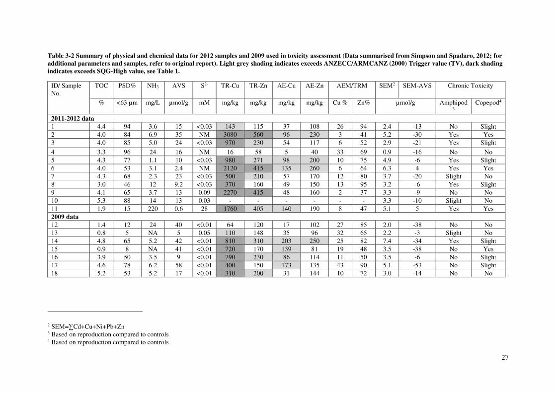
Table 3-2 Summary of physical and chemical data for 2012 samples and 2009 used in toxicity assessment (Data summarised from Simpson and Spadaro, 2012; for additional parameters and samples, refer to original report). Light grey shading indicates exceeds ANZECC/ARMCANZ (2000) Trigger value (TV), dark shading indicates exceeds SQG-High value, see Table 1. .................................................................. 27

Table 3-3 Scenarios used to investigate the contribution of copper and zinc to observed toxicity in chronic amphipod and copepod bioassays. .............................................................................................................. 29

Table 3-4 Options considered for setting management limits for sediments contaminated by copper-based antifoulant paint (Taken from Simpson and Spadaro, 2012). ..................................................................... 29

Table 3-5 Trigger values for toxicants at varying levels of protection for marine systems (ANZECC/ARMCANZ, 2000). .................................................................................................................. 32

Table 3-6 Mean sediment copper concentrations (mg/ kg) for individual sites sampled in Huon Estuary and D’Entrecasteaux Channel as part of DPIPWE compliance monitoring, and studies by Jones (2000) and Macleod and Helidoniotis (2005). ........................................................................................................ 51

Table 3-7 Comparison of data available between farm based monitoring data and Jones (2000) and Macleod and Helidoniotis (2005) datasets. ................................................................................................. 52

Table 3-8 Comparison of actual versus predicted copper concentrations for sites sampled by Macleod and Helidoniotis (NRM, 2004) based on relationship with organic matter content (OM, by LOI) identified in farm based control monitoring data (y=1.2332x + 3.1861). ....................................................................... 55

Table 3-9 Average total recoverable copper concentrations (Mean TR-Cu) for farm monitoring control sites in the Huon Estuary and D’Entrecasteaux Channel showing related percentage silt-clay (<63um) and Shannon diversity (H’) measures and associated correlation coefficients. ................................................. 59

Table 3-10. Average total recoverable copper concentrations (TR-Cu) for sediments from both control locations and sediment traps at the study sites, and the average TR-Cu concentration for sediments from the Huon Estuary region with a similar organic carbon content. ................................................................ 62

v

List of Figures

Figure 1-1 Potential pathways for deposition and uptake of copper associated with marine farming (modified from Eriksen and Macleod, 2009). ............................................................................................... 2

Figure 1-2 Tiered framework (decision tree) for the assessment of contaminated sediments for metals (ANZECC/ARMCANZ 2000). ..................................................................................................................... 6

Figure 2-1 Map of Sample sites for Objective 1 studies (Blue = Treatment 1, Red = Treatment 2). ......... 12

Figure 2-2 Schematic of sampling locations, 4 cardinal samples on the pen bay perimeter and on central sample. ......................................................................................................................................................... 13

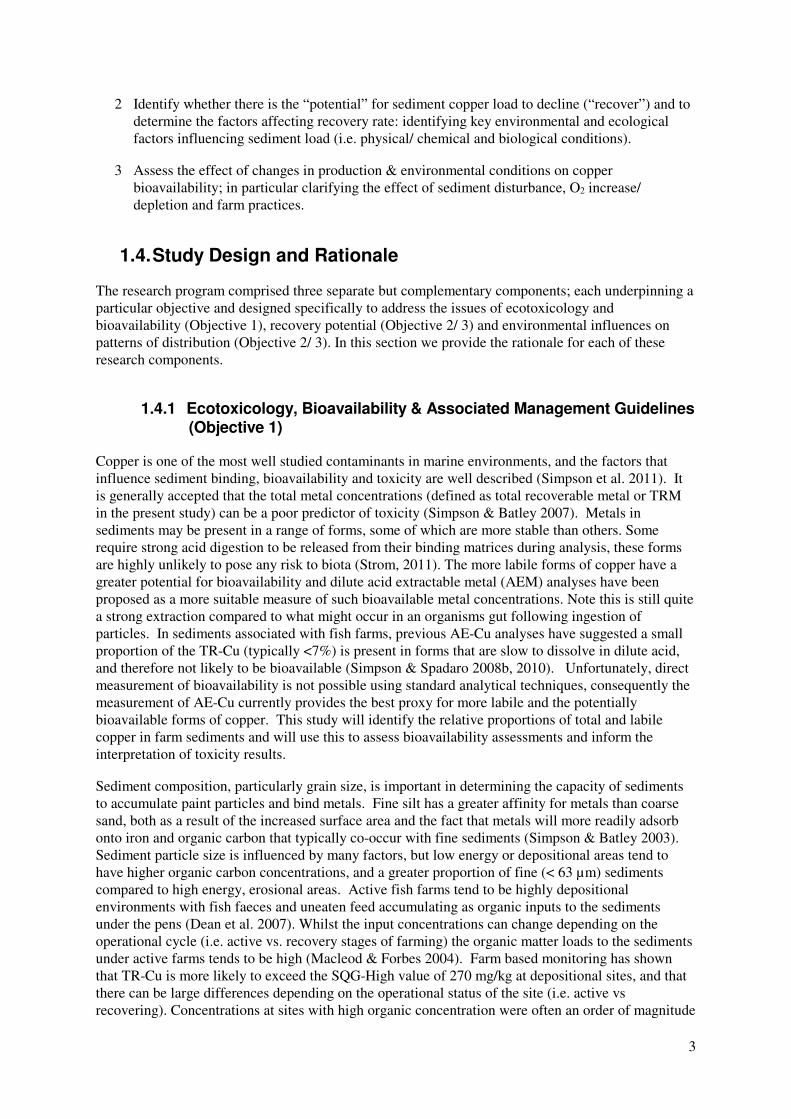
Figure 2-3 Multicore sampling device for mini cores (left) and an individual core sealed with latex bungs (right) used for metals sampling. ................................................................................................................. 15

Figure 2-4 Spade corer (left) and Craib corer (right). ................................................................................. 15

Figure 2-5 Box core (left) and Perspex liner (right) used for bulk sediment sampling. ............................. 15

Figure 2-6 Perspex grab liner (left) and individual mesocosm core sub-sampled from liner (right). ......... 17

Figure 2-7 Mesocosm cores equilibrating with spacers under lids (left) and sealed and submerged during incubation (right). ........................................................................................................................................ 18

Figure 2-8 Sediment trap locations (black labels), Huon River, in relation to temporal farm sites (grey labels, Tasman Peninsula not shown for clarity). ....................................................................................... 20

Figure 2-9 Sediment trap locations relative to shore and lease boundaries. ............................................... 20

Figure 2-10 Sediment traps (note: 50ml container attached to the side of each core for collection of metal samples) ....................................................................................................................................................... 21

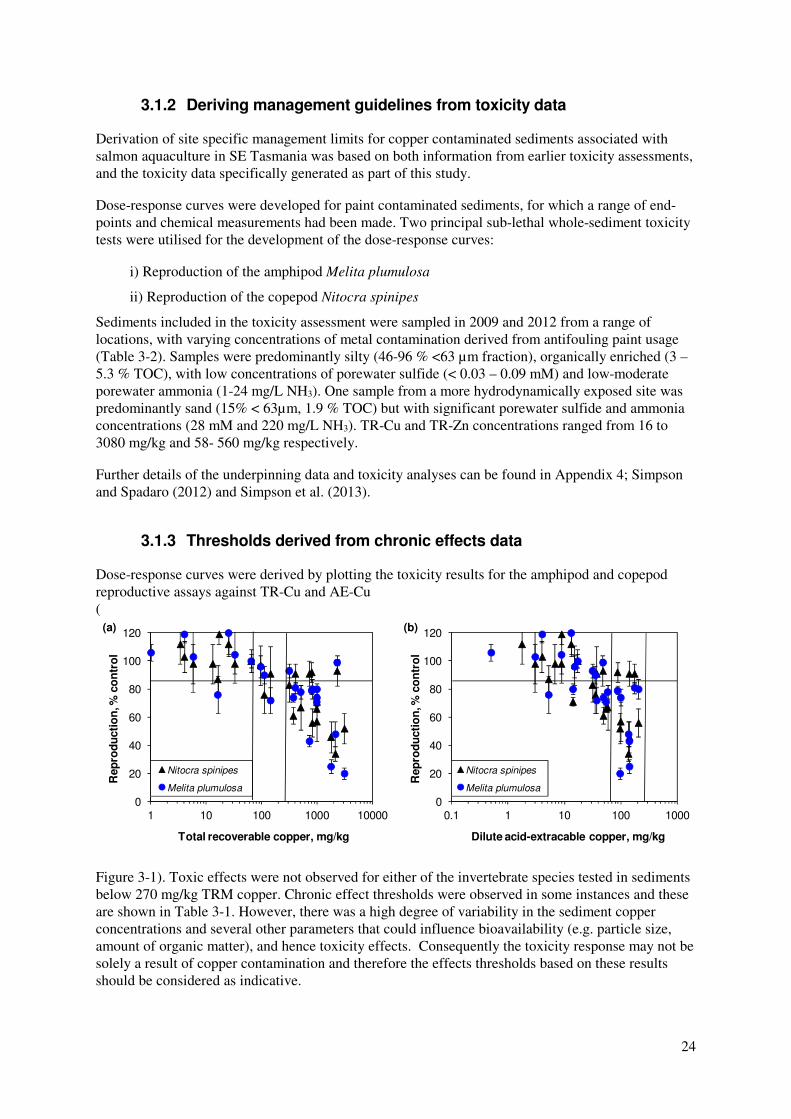
Figure 3-1. Relationship between toxicity (inhibition of reproduction) in the amphipod and copepod bioassays and a) TR-Cu, and b) AE-Cu. Reproduced from Simpson et al. (2013). .................................... 25

Figure 3-2 Relationships between the observed toxicity and a range of calculated SQGQs. The 15% and 25% effects limits (considered to be no effects limits) are shown as horizontal lines for M. plumulosa and N. spinipes, respectively. Data to the left of the SQGQ = 1 line suggest the guideline may not be adequately protective, while data to the rights of the line is adequate, or overly protective. Data from this study and Simpson and Spadaro (2011). ..................................................................................................... 28

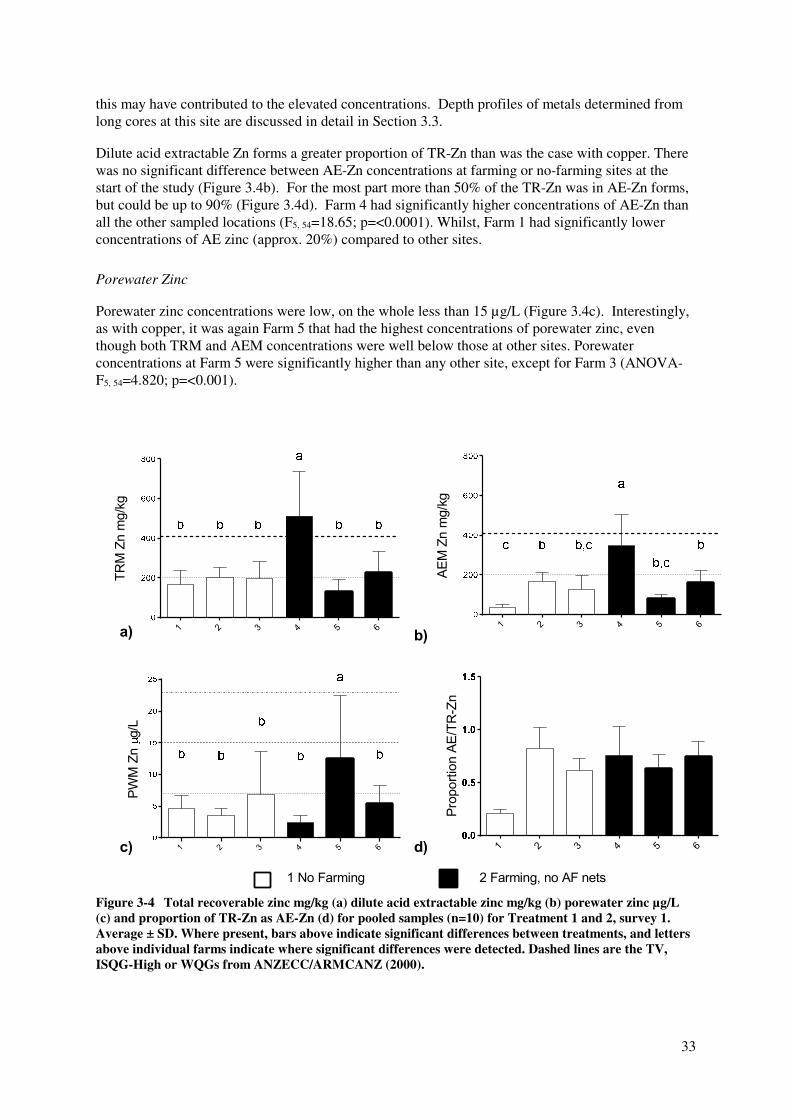
Figure 3-3 Total recoverable copper mg/kg (a) dilute acid extractable copper mg/kg (b) porewater zinc µg/L (c) and proportion of TR-Cu as AE-Cu (d) for pooled samples (n=10) for Treatment 1 and 2, survey 1. Average ± SD. Where present, bars above indicate significant differences between treatments, and letters above individual farms indicates where significant differences were detected. Dashed lines are the TV, ISQG-High or WQGs from ANZECC/ARMCANZ (2000). ............................................................... 31

Figure 3-4 Total recoverable zinc mg/kg (a) dilute acid extractable zinc mg/kg (b) porewater zinc µg/L (c) and proportion of TR-Zn as AE-Zn (d) for pooled samples (n=10) for Treatment 1 and 2, survey 1. Average ± SD. Where present, bars above indicate significant differences between treatments, and letters above individual farms indicate where significant differences were detected. Dashed lines are the TV, ISQG-High or WQGs from ANZECC/ARMCANZ (2000). ............................................................... 33

vi

Figure 3-5 Total recoverable (TR) vs. a) dilute acid extractable (AE) and b) porewater (PW) copper for all samples from survey 1, temporal study and TR-Cu vs. AE-Cu for c) treatment 1 (No farming) and d) treatment 2 (Farming) locations separately. ................................................................................................ 34

Figure 3-6 AEM vs porewater Copper for survey 1, temporal study. ................................................... 35

Figure 3-7 TRM vs a) acid extractable (AEM), b) porewater (PW) and c) AEM versus porewater zinc for survey 1, temporal study. ............................................................................................................................ 35

Figure 3-8 Bulk sediment properties: a) TOC mg/kg b) PS < 63 µm and c) AVS for pooled samples (n=10) for Treatment 1 and 2, survey 1. Average ± SD. Where present, bars above indicate significant differences between treatments, and letters above individual farms indicate where significant differences were detected. ............................................................................................................................................. 36

Figure 3-9 a) Ammonia and b) Nitrate flux µM-N/m2/hr c) phosphate flux µM-P/m2/hr and d) Oxygen flux µM/m2/hr for pooled samples (n=10) for Treatment 1 and 2, survey 1. Average ± SD. Where present, bars above indicate significant differences between treatments, and letters above individual farms indicate where significant differences were detected. .............................................................................................. 38

Figure 3-10 Concentrations of total, dilute acid extractable and porewater copper at each farm and time for which there is data. ANZECC/ARMCANZ (2000) guideline values (sediment, water) shown for reference. 41

Figure 3-11 Concentrations of a) total, b) dilute acid extractable and c) porewater zinc at each farm and time, for which there is data. ANZECC/ARMCANZ (2000) guideline values (sediment, water) shown for reference. 42

Figure 3-12 Flux rates for ammonia, NOx and oxygen at each farm and time. Note that fluxes were not measured at time 2 (6 months into study period). ....................................................................................... 43

Figure 3-13 Concentrations of total recoverable copper through time for each pen bay at a) ‘no farming’ and b) ‘farming’ sites, temporal study Arrows indicate when farming ceased (or net cleaning in the case of Farm 3a). Farm 1 vacant since March 2008. ............................................................................. 44

Figure 3-14 Concentrations of total recoverable copper through time pooled from all samples collected in each year at Farm 1. ................................................................................................................................ 45

Figure 3-15 Total recoverable copper and zinc concentrations (mg/kg) for each of the duplicate cores collected from Farm 4 and Farm 7 a) Farm 4 (Cage), b) Farm 4 (Compliance), c) Farm 7 (Cage) ) and d) Farm 7 (Compliance)................................................................................................................................... 47

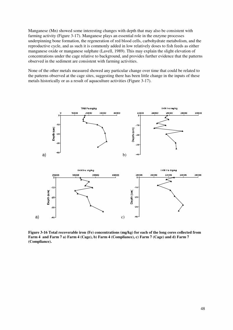
Figure 3-16 Total recoverable iron (Fe) concentrations (mg/kg) for each of the long cores collected from Farm 4 and Farm 7 a) Farm 4 (Cage), b) Farm 4 (Compliance), c) Farm 7 (Cage) and d) Farm 7 (Compliance). .............................................................................................................................................. 48

Figure 3-17 Total Recoverable arsenic (As), cadmium (Cd), cobalt (Co), chromium (Cr), manganese (Mn), nickel (Ni) and lead (Pb) concentrations (mg/kg) for each of the long cores collected from Farm 4 and Farm 7 a) Farm 4 (Cage), b) Farm 4 (Compliance), c) Farm 7 (Cage) and d) Farm 7 (Compliance). . 49

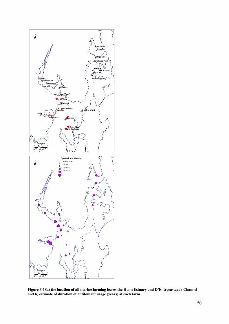
Figure 3-18a) the location of all marine farming leases the Huon Estuary and D’Entrecasteaux Channel and b) estimate of duration of antifoulant usage (years) at each farm. ....................................................... 50

Figure 3-19 Concentrations of copper (mg/kg DMB) in sediments at farm control sites from the Huon Estuary and D’Entrecasteaux Channel in relation to the associated concentrations of a) redox, b) silt-clay and c) organic content. ................................................................................................................................ 53

vii

Figure 3-20 Concentrations of copper in sediments at farm control sites from the Huon estuary and D’Entrecasteaux Channel in relation to the associated biological factors: a) number of taxa, b) number of individuals and c) Shannon diversity. ......................................................................................................... 54

Figure 3-21 Concentrations of copper compared with depth at a) farm control sites from the Huon estuary and D’Entrecasteaux Channel and b) all sites sampled for farm control studies as well as previous monitoring studies by Jones (2000) and Macleod and Helidoniotis ( 2005). ............................................. 54

Figure 3-22 Total recoverable copper concentration versus % organic matter (OM) content for both farm and control sites in the Huon estuary and D’Entrecasteaux Channel. ........................................................ 56

Figure 3-23 Location of controls sites in the Huon Estuary and D’Entrecasteaux Channel showing a) average total recoverable copper concentrations for each site, b) number of fish farms within a 15 km radius of each control site and c) the weighted potential influence of farm sites on each of the control sites . .................................................................................................................................................................... 57

Figure 3-24 Rate of change (% annually) in total recoverable copper concentrations for each control site; green dots indicate where copper concentrations have decreased whilst red/ orange dots indicate where copper values have increased. ..................................................................................................................... 58

Figure 3-25 Average total recoverable copper concentrations for each control site compared with a) total number of farms within 15 km of control site, b) weighted farm exposure index. ..................................... 58

Figure 3-26 Ordination (Multidimensional scaling) plot of farm monitoring control sites in the D’Entrecasteaux Channel (1), Huon Estuary (2) and Tasman Peninsula (3) based on benthic community structure with a) TR copper levels for each site , b) percentage silt-clay (<63um) and c) % organic content (LOI) overlaid as bubble plots. ................................................................................................................... 60

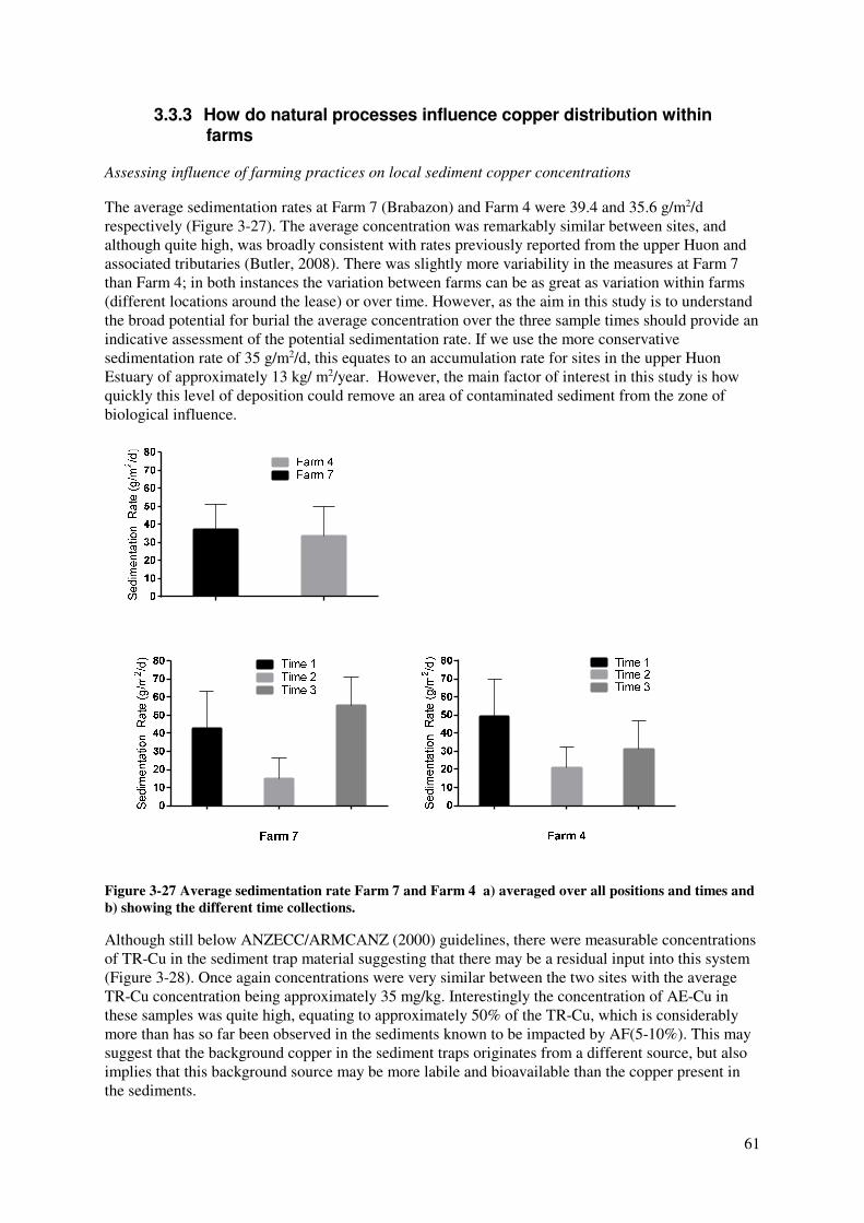
Figure 3-27 Average sedimentation rate Farm 7 and Farm 4 a) averaged over all positions and times and b) showing the different time collections. ................................................................................................... 61

Figure 3-28 a) Average total recoverable (TR-Cu) and b) average dilute acid extractable copper (AE-Cu) at Farm 7 and Farm 4. ................................................................................................................................. 62

viii

Acknowledgments

Matt Barrenger, Linda Sams, Cameron Dalgleish, Damien Strong, Sam Kruimink and Ben Quiggly (Tassal); Adam Main (TSGA); Dom O’Brien (HAC); Eric Brain, Graham Woods, and Marc Santo (DPIPWE); Andrew Pender, Bronagh Kelly, Lisette Robertson, Malinda Auluck, Tom Clifford, Alan Beech (IMAS); David Spadaro, Ian Hamilton and Chad Jarolimek (CSIRO); Joe Valentine and Jeremy Lane (Aquenal)

Abbreviations

AEM Dilute Acid Extractable Metal (1 M HCl)

AE-Cu Dilute Acid Extractable Copper Concentration

AE-Zn Dilute Acid Extractable Zinc Concentration

AF Antifoulant

ANZECC Australian and New Zealand Environment Conservation Council

ARMCANZ Agriculture and Resource Management Council of Australia and New Zealand

APVMA Australian Pesticide and Veterinary Medicines Authority

AST Analytical Services Tasmania

AVS Acid Volatile Sulfides

CSIRO Commonwealth Scientific and Industrial Research Organisation

CTD Conductivity Temperature Depth

Cu Copper

DMB Dry Matter Basis

DPIPWE Department of Primary Industries, Parks, Water and Environment

EC50 Effective Concentration (at which 50% of the population are affected)

ISQG Interim Sediment Quality Guideline

LOI Loss On Ignition

MDS Multi-Dimensional Scaling

OPD Oxygen Penetration Depth

PSD Particle Size Distribution

PW Pore Water

SQG Sediment Quality Guideline

SQGQ SQG Quotients

ix

TOC Total Organic Carbon

TRM Total Recoverable Metal

TR-Cu Total Recoverable Copper Concentration

TR-Zn Total Recoverable Zinc Concentration

TSGA Tasmanian Salmonid Growers Association

TV Trigger Value (same as ISQG-Low value)

Zn Zinc

x

Executive Summary

What the report is about

Farm based monitoring has shown copper concentrations in sediments under salmon farms in the Huon and D’Entrecasteaux Channel are elevated relative to background conditions as a result of long-term use of copper-based antifoulants. This study was undertaken as a collaboration between researchers at the Institute for Marine and Antarctic Studies (University of Tasmania) and CSIRO, and with the cooperation of the Tasmanian Salmon farming industry to determine whether these copper concentrations have any major or long-term impacts on the local ecology or sediment function and to identify the remediation potential of these sediments and what, if any, management strategies could be used to enhance recovery. Noting that in this instance recovery was assessed as either i) a marked decline in copper over time (recovery in progress) or ii) return to background/ baseline copper concentrations (total recovery).

Conditions were assessed over the short-term (12 months, this study) at sites selected for high copper loads, as well as over the longer-term (> 5 years, incorporating the results of previous farm-based assessments) at sites where the copper concentration history was well-known. Changes in background concentrations were assessed by reviewing copper data from both the farm assessments and a range of previous studies in the region, and integrating broader environmental data on prevailing conditions and exposure. Finally, targeted sedimentation studies provided data on deposition and accumulation rates that could be used to provide longer-term projections for recovery.

A specific concern at the start of this study was that ongoing farming, even without the use of antifoulant nets, could increase the risk of toxicity in sediments where copper concentrations were elevated; the results of this study clearly identify that this is not the case. The results indicate that the risk of serious adverse impacts on sediment processes from current copper contamination levels is relatively low; largely because most of the copper occurs as paint flakes and can’t be easily taken up by benthic organisms.

Copper can exist in a variety of forms in the sediments, with some being more toxic than others. The concentrations of relevant forms of copper were assessed, and the associated sediment conditions determined. Whilst antifoulant usage was shown to be the primary source of elevated copper concentrations within farms, local environmental conditions and certain farming practices can have a significant influence on copper accumulation and impact levels throughout the system. Consequently, it was possible to make operational management recommendations that will reduce the potential for impacts into the future. The study also recommends refined regulatory guidelines that should provide better protection with respect to chronic ecotoxicological impacts.

Background

This project arose out of discussions between industry, relevant state and federal regulators and researchers regarding the management of copper residues in sediments as a result of copper based antifoulant use on salmon net-pens. Copper-based antifoulant has been used extensively within the industry over the last 10 years (FRDC project 2007/246), but it was only when industry monitoring of sediments showed that concentrations were above ANZECC/ARMCANZ (2000) guidelines at certain sites that concern grew as to whether this might have ecological impacts. A study to identify the ecological effects of contamination indicated that most of the copper was associated with paint flakes and that toxicity, even in the most highly contaminated sediments was quite low (FRDC project 2009/218). However, subsequent industry based monitoring results suggested that accumulation in some areas/ sites was greater than had previously been predicted, and there was some concern that changes in the sediment biogeochemistry associated with changes in farming operations (i.e. active farming versus fallowing) might influence toxicity. As a result this study was commissioned to better understand the impact of existing sediment residues, the potential for sediment recovery and the effect of changing operational and environmental conditions on copper bioavailability.

xi

Aims/ Objectives

The aims of this study were threefold:

1 Identify the effect of existing sediment copper concentrations and recommend management guidelines: i) Establishing dose-response relationships based on chronic effects to benthic organisms, ii) Evaluating the potential hazard associated with aquaculture sediments

2 To identify whether there is the “potential” for sediment copper load to decline (“recover”) and to determine the factors affecting recovery rate: identifying key environmental and ecological factors influencing sediment load (i.e. physical/ chemical and biological conditions)

3 To assess the effect of changes in production & environmental conditions on copper bioavailability; in particular clarifying the effect of sediment disturbance, O2 increase/depletion and farm practices.

Copper Guideline Values

The ANZECC/ARMCANZ (2000) sediment quality guidelines (SQGs) are used in this report. For copper, there are two interim SQG values; a low value of 65 mg/kg (ISQG-Low), also known as the trigger value (TV) and a high value of 270 mg/kg (the ISQG-High). When referring to these guideline values, the terms TV and ISQG-High will be used to refer to 65 and 270 mg/kg, respectively. All concentrations in assessments are referred to on a dry weight basis.

Methods

The research program comprised three separate but complementary components; these underpinned the objectives outlined above and were designed specifically to address the issues of ecotoxicology and bioavailability (Objective 1), recovery potential (Objective 2/ 3) and environmental influences on patterns of distribution (Objective 2/ 3).

Ecotoxicology, Bioavailability & Associated Management Guidelines (Objective 1)

This first component sought to address the issue of toxicity and copper bioavailability in relation to highly contaminated farm sediments. Sediment samples were collected from a range of contamination levels (identified from the results of farm-based monitoring assessments), specific toxicity tests were undertaken and the nature of the copper in the sediments was assessed.

This provided an evaluation of both acute and chronic toxicity at the most contaminated sites as well as an assessment of the relationship between total and chemical estimates of potentially bioavailable copper concentrations.

Recovery Potential & Associated Management Guidelines (Objective 2/ 3)

Recovery potential was assessed at a total of 6 sites where the sediment copper concentrations were above the ISQG-High (270 mg/kg).

Three sites were selected for two differing treatments.

Treatment 1 (fallowed) - the sites would have no farming activity for the duration of the study.

Treatment 2 (farmed) - the sites would be farmed normally but without antifouled nets.

In each case changes in the sediment conditions and copper concentrations were assessed at intervals over 12 months. As part of that assessment any changes in copper form/ speciation within the sediments over the farming and fallowing cycles was noted.

In addition, at two sites further samples were collected to assess sediment deposition and accumulation rates. Sediment traps were deployed at 3 positions and at 3 times within the lease to evaluate background

xii

deposition rates, and long cores were collected to examine the vertical distribution (and hence longer-term accumulation) of metals within the sediments.

Broadscale Influences & Associated Management Guidelines (Objective 2/ 3)

The third component examined the effect of changing environmental conditions on background copper concentrations and the deposition of copper within the broader ecosystem. This study involved a meta-analysis of the existing farm monitoring data and two other datasets where comparable data existed on the copper concentrations and environmental conditions in the Huon and D’Entrecasteaux Channel system (Jones, 2004 and Macleod and Helidoniotis, 2005)

The primary aim of this component was to identify any environmental conditions that might pre-dispose an area to copper accumulation. As part of this broadscale assessment a further additional goal was added after the study commenced, this was to evaluate whether there was any evidence of copper accumulation in the broader environment that might be related to the presence of farming within the system

Copper concentrations were assessed as bulk sediment loads, as well as porewater and solid phase (dilute acid extractable and total recoverable) metal concentrations. Measures of sediment function were based around evaluation of nutrient fluxes (ammonia, phosphate, nitrate/nitrite), oxygen flux and an assessment of community changes. In addition other aspects of the sediments that are known to be highly influential in determining both deposition and metal bioavailability such as oxygen penetration, acid volatile sulphide concentrations, particle size and organic carbon content were assessed. Industry also provided data on farming conditions.

Results/ Key findings

Objective 1 Identify the effect of existing sediment copper concentrations and recommend management guidelines: i) Establishing dose-response relationships based on chronic effects to benthic organisms, ii) Evaluating the potential hazard associated with aquaculture sediments

The proportion of the total copper concentration that is potentially bioavailable was estimated to be relatively small based on dilute acid extractable copper concentrations (AE-Cu). Toxicity testing showed no evidence of any acute toxicity effects as a result of farm-derived copper inputs nor was there any evidence of any significant change in benthic community composition or ecosystem function (nutrient processing) where copper concentrations were elevated. However, there was potential for chronic toxicity and consequently it is proposed that the current monitoring requirements be adjusted, such that where total recoverable copper concentrations (TR-Cu) exceed the ISQG-High (270 mg/kg), then additional sampling be undertaken to ensure that AE-Cu concentrations do not exceed the TV (65 mg/kg). This should provide adequate protection for ecosystem health.

Objective 2 To identify whether there is the “potential” for sediment copper load to decline (“recover”) and to determine the factors affecting recovery rate: identifying key environmental and ecological factors influencing sediment load (i.e. physical/ chemical and biological conditions).

There was no evidence from the short-term recovery studies (12 months) that sediments had returned to background/ baseline concentrations (total recovery) or that there had been any significant decline over time (recovery in progress). However, evaluation of farm data (>5 yrs) and the results of the long cores suggest that there is potential for recovery over the longer term. The prevailing environmental conditions at a site, and its’ depositional status are the key determinants of metal concentration; with organic content being the best indicator of the depositional risk. It is proposed that copper based antifoulant nets are not used at sites where organic matter concentrations (LOI) are greater than 15%.

xiii

Objective 3 To assess the effect of changes in production & environmental conditions on copper bioavailability;

The presence of copper in the sediments did not have any significant effect on the normal biogeochemical processes or ecosystem function, regardless of whether sites were farmed or fallowed. Consequently, it is sufficient to require copper based nets to be removed where sediment copper concentrations exceed proposed management levels; farming itself can continue so long as non-antifouled nets are used. Additional management recommendations included the need to either avoid significant net manipulations (bending, folding or crowding), or where such activities are essential, use non-antifouled nets.

Implications for relevant stakeholders

Industry – this study has identified some clear management actions that would reduce the impact of copper antifouled nets. However, it is important to acknowledge that industry have been involved in this study from the outset and as such have implemented many actions already based on the findings as they became known. Consequently the industry has made the decision to replace all nets coated with copper based antifoulants and this process should be completed by 2015.

Managers or policy makers – This report contains details of specific changes to monitoring requirements and recommendations on restrictions for usage of copper based antifoulants in salmon aquaculture that will inform management protocols. It also identifies that the current management level of 270 mg/kg remains a meaningful trigger based on bioavailability results for antifoulant paint in sediments.

Recommendations

Recommendations have already been detailed in the results/ findings section above, but are summarised here for each stakeholder group as follows:

Farm practices

• Minimise use of copper based antifoulants at all sites, and look to replace any nets at farms where there is evidence of metal accumulation in sediments.

• Minimise net manipulations and potential for abrasion, but for activities where this cannot be avoided (i.e. fish crowding/ transfer) then replace with non-antifouled nets.

• Increase use of monofilament/ plastic nets wherever possible, but especially at depositional sites, where organic content (LOI) is >15% (suggest that copper based antifoulants should only be used at sites where organic content is <15%).

Monitoring

• Where total recoverable copper concentrations in the sediments exceed the ISQG-High (270 mg/kg) then dilute acid extractable copper concentration should also be assessed to ensure that concentrations are below the TV (65 mg/kg).

• Continue to measure total recoverable copper – this is necessary for consistency with historical datasets and protocols, and therefore essential for assessment of recovery.

Other Issues

Although zinc was not a key focus of this study, and there was no evidence of specific toxicity or particular ecological concerns at the concentrations observed. However, zinc concentrations were quite high at a number of sites. As zinc accumulation is not solely associated with antifoulant usage, (it is also included as a nutritional supplement in fish feed), then the management recommendations pertaining to copper may not be effective for zinc. Consequently it is suggested it may be prudent to continue monitoring zinc concentrations.

xiv

Keywords

Salmon aquaculture, Salmo salar, sediment, antifouling, paint, sediment, copper, zinc, benthic processes, recovery, environmental management

1

1 Introduction

1.1. Background

Preventing biofouling on fish farm nets is critical to maintaining good water flow, ensuring high dissolved oxygen concentrations, and maintaining fish health. One means of achieving this is through the use of antifouling paints. Since 2003 a variety of antifouling products have been trialled on nets at farms in South East Tasmania. Initial industry trials had identified copper based paints as the most cost-effective product for management of biofouling (O’Brien et al. 2009). Copper-based paints have the additional advantage of adding significant rigidity to nets (stiffening), improving resistance of nets to seal attack, and providing some relief from costly maintenance of barrier-defence systems (Macleod & Eriksen 2009). There are two main copper based paint products currently used under permit in Tasmania, these contain either 12.5-15% copper as Cu2O (half-strength product), or 25-50% copper (full-strength product) as the primary active ingredient (Macleod and Eriksen, 2009. These paints also contain zinc oxide (~5%) to control the rate of coating erosion.

Copper-based antifouling paints are designed to slowly, but continually, release copper into the water column and this acts as a deterrent to marine fauna and flora settling on the nets. Therefore it is to be expected that copper concentrations may be elevated in the water column close to painted structures (Yebra et al. 2004). The environmental risk posed by paint-derived metals in waters is strongly linked to the local water flow regime. While dilution may be reduced in enclosed areas such as marinas (Schiff et al. 2007), the higher water flows required in fish aquaculture areas mean that water quality guidelines (WQGs) are typically not exceeded However, there are a number of pathways by which copper can be accumulated in sediments and the water column (Figure 1-1). Highly elevated concentrations of copper in sediments within fish farms have been attributed to the deposition of paint flakes as a result of in-situ cleaning, improperly dried or coated nets, and abrasive marine operations (O’Brien et al. 2009). In-situ cleaning of nets has been addressed, in part, through the development of best practice guidelines recommending suction rather than blast cleaning for antifouled nets (TSGA 2013) but concentrations in some sediments remain high.

Use of antifouling products in South East Tasmania is permitted under Research Permit 10924, granted by the APVMA, and renewed annually. This permit allows for the supply and use of an unregistered AGVET product, for the purpose of assessing the potential for accumulation of copper in sediments, in and around fish farms. Ongoing use and full registration of the paint in Australia by the APVMA is dependent upon developing a sound understanding of the environmental hazard and potential impacts associated with copper contamination of sediments by these products.

1.2. Need

Industry monitoring identified sizeable increases in sediment concentration of copper at farm sites in the Huon and D’Entrecasteaux Channel, with concentrations at some sites exceeding current national standards and environmental management levels for sediment copper concentrations (ANZECC/ARMCANZ 2000). Both industry and environmental regulators recognised that this was a significant concern and identified a need to better define the potential for environmental impacts associated with copper contamination, identify the conditions that affect copper build up under cages, and develop a strategy for management and remediation of these sediments.

While there was some evidence to suggest that paint-associated copper in sediments may be less readily bioavailable than other forms, this needed to be clarified. Research needed to be undertaken to i) establish whether elevated copper concentrations associated with fish farms are having an

2

adverse impact on either benthic ecology or sediment function, ii) determine how local environmental conditions and ongoing farming activities might affect this, and iii) evaluate the potential for recovery (i.e. timeframe and conditions required).

The current SQGs for management of metals are generally considered to be quite conservative. The intention of the SQGs is to promote a better understanding of the contamination issue, with the TV and ISQG-High values being used in the initial phases of assessment framework (as a screening tool) to trigger additional investigations if exceeded (Batley & Simpson 2008). Consequently, with sufficient evidence it may be feasible to propose alternative management criteria that are more effective for managing the copper contamination resulting from antifouling paint.

Figure 1-1 Potential pathways for deposition and uptake of copper associated with marine farming

(modified from Eriksen and Macleod, 2009).

Accordingly, it was determined that there was a need to: identify reliable approaches for monitoring copper bioavailability; ascertain the potential for natural or assisted remediation (does it occur and can it be managed); and to understand the implications of farm management practices on sediment contamination (e.g. organic enrichment, fallowing). This information will enable the development and implementation of risk appropriate management strategies.

1.3. Objectives

Three objectives were defined for this project:

1 Identify the effect of existing sediment copper concentrations and recommend management guidelines: i) establishing dose-response relationships based on chronic effects to benthic organisms, ii) evaluating the potential hazard associated with aquaculture sediments.

3

2 Identify whether there is the “potential” for sediment copper load to decline (“recover”) and to determine the factors affecting recovery rate: identifying key environmental and ecological factors influencing sediment load (i.e. physical/ chemical and biological conditions).

3 Assess the effect of changes in production & environmental conditions on copper bioavailability; in particular clarifying the effect of sediment disturbance, O2 increase/ depletion and farm practices.

1.4. Study Design and Rationale

The research program comprised three separate but complementary components; each underpinning a particular objective and designed specifically to address the issues of ecotoxicology and bioavailability (Objective 1), recovery potential (Objective 2/ 3) and environmental influences on patterns of distribution (Objective 2/ 3). In this section we provide the rationale for each of these research components.

1.4.1 Ecotoxicology, Bioavailability & Associated Management Guidelines (Objective 1)

Copper is one of the most well studied contaminants in marine environments, and the factors that influence sediment binding, bioavailability and toxicity are well described (Simpson et al. 2011). It is generally accepted that the total metal concentrations (defined as total recoverable metal or TRM in the present study) can be a poor predictor of toxicity (Simpson & Batley 2007). Metals in sediments may be present in a range of forms, some of which are more stable than others. Some require strong acid digestion to be released from their binding matrices during analysis, these forms are highly unlikely to pose any risk to biota (Strom, 2011). The more labile forms of copper have a greater potential for bioavailability and dilute acid extractable metal (AEM) analyses have been proposed as a more suitable measure of such bioavailable metal concentrations. Note this is still quite a strong extraction compared to what might occur in an organisms gut following ingestion of particles. In sediments associated with fish farms, previous AE-Cu analyses have suggested a small proportion of the TR-Cu (typically <7%) is present in forms that are slow to dissolve in dilute acid, and therefore not likely to be bioavailable (Simpson & Spadaro 2008b, 2010). Unfortunately, direct measurement of bioavailability is not possible using standard analytical techniques, consequently the measurement of AE-Cu currently provides the best proxy for more labile and the potentially bioavailable forms of copper. This study will identify the relative proportions of total and labile copper in farm sediments and will use this to assess bioavailability assessments and inform the interpretation of toxicity results.

Sediment composition, particularly grain size, is important in determining the capacity of sediments to accumulate paint particles and bind metals. Fine silt has a greater affinity for metals than coarse sand, both as a result of the increased surface area and the fact that metals will more readily adsorb onto iron and organic carbon that typically co-occur with fine sediments (Simpson & Batley 2003). Sediment particle size is influenced by many factors, but low energy or depositional areas tend to have higher organic carbon concentrations, and a greater proportion of fine (< 63 µm) sediments compared to high energy, erosional areas. Active fish farms tend to be highly depositional environments with fish faeces and uneaten feed accumulating as organic inputs to the sediments under the pens (Dean et al. 2007). Whilst the input concentrations can change depending on the operational cycle (i.e. active vs. recovery stages of farming) the organic matter loads to the sediments under active farms tends to be high (Macleod & Forbes 2004). Farm based monitoring has shown that TR-Cu is more likely to exceed the SQG-High value of 270 mg/kg at depositional sites, and that there can be large differences depending on the operational status of the site (i.e. active vs recovering). Concentrations at sites with high organic concentration were often an order of magnitude

4

greater than at comparable high energy sites with low organic carbon concentrations. This supports the hypothesis that paint particles and dissolved copper have a greater affinity for sediments at depositional sites (Simpson & Spadaro 2008b, Macleod & Eriksen 2009, Simpson & Spadaro 2010). Interestingly, there is also a high degree of small scale spatial heterogeneity in copper distribution (i.e. within pen bay footprints), which is also consistent with the premise of paint flakes as the primary source (Eriksen & Macleod 2011). The influence of farming activities and environmental differences on copper speciation and bioavailability will be further explored.

Previous studies of these particular fish farm sediments have shown that a relatively large proportion of the total copper (45-92%) in sediment was associated with particles larger than 63 µm (Simpson & Spadaro 2008b, Dalgleish, unpublished data 2009), suggesting that much of the copper contamination may be associated with paint particles, as dissolved copper from the nets would be expected to adsorb preferentially to the finer sediment particles. Locations where intensive net handling operations such as net changes, crowding or grading occur have been shown to have greater sediment concentrations to the sediment (Macleod & Eriksen 2009, O’Brien et al. 2009, Simpson & Spadaro 2013). The transformation of the copper (I) oxide in the paint matrix to more bioavailable forms will be strongly influenced by paint’s leaching rate (Eriksen & Macleod 2011). Antifoulant paints are designed to work most effectively where their release is facilitated by water movement. Buried in sediment, in the absence of mixing currents, the release rate of copper will be governed by diffusional fluxes to pore waters and eventually to overlying waters. Consequently, it may not be surprising that the majority of copper in the sediments at fish farms was still in the particulate form, rather than having dissolved and re-adsorbed to the sediment. This however has further implications for the fate of copper, and the potential for recovery and targeted studies have been outlined to examine these factors; these are addressed more fully in the following sections.

Weathering increases the bioavailability of paint-associated copper (Simpson and Spadaro, 2010). The percentage of TRM present as AE copper was higher in nets deployed for 6 (47%) and 12 months (57%) compared to freshly painted nets (17%). Effects of UV and dry storage on paint leaching rates were identified as possible factors for further investigation (Simpson and Spadaro, 2010). Release rates for particles removed from net material will be greater than the paint itself due to the increased surface area of the particles. However, release rates of particles in sediment will be reduced due to limitations on diffusion from being buried and sediment conditions which are likely to bind the metals. Consequently, age and history of paint, including weathering, are likely to be important factors in determining copper release rates and bioavailability once paint flakes are deposited in sediments.

The oxic status of the sediments has a marked influence on bioavailability and copper release, with copper tending to be bound more strongly in anoxic sediments. Fine, silty sediments rich in organic carbon have a tendency to be sub-oxic or anoxic (Glud 2008). Organic enrichment of the sediments associated with fish farm wastes will rapidly become anoxic (Macleod et al., 2004,2007, Eriksen et al. 2012). This results in anaerobic processes dominating, with sulphate reducing bacteria producing sulphides which can effectively remove copper from the labile or bioavailable pool as insoluble copper sulphide. Acid volatile sulfide (AVS) concentration provides a useful measure of sulphide binding capacity; where the AVS concentration is greater than the copper concentration then very low concentrations of copper in pore waters should result (Simpson et al. 2000). However, it is important to note that the binding of copper in sulphide forms is reversible if/ when sediments become oxidised again. Oxidation of sediments via resuspension or natural recovery processes can result in the release of copper into the water column, and potentially back into the bioavailable pool (Simpson et al., 1998; Simpson and Batley, 2003). Consequently in the present study the impact of changing environmental and farm management condition on copper bioavailability was assessed.

The toxicity of copper in any environment is a function of the level of contamination, bioavailability and opportunity for exposure. Organisms that reside in or on the sediment will have different exposure risk concentrations, depending upon their ecological niche, and relative importance of the

5

two primary uptake routes - dissolved and dietary (Simpson & Spadaro 2011). Organisms that are in contact with overlying waters, pore waters, or that irrigate their burrows will be more vulnerable to exposure to dissolved metals. Feeding physiology (filter feeders, detrital scavengers etc.) and factors such as gut passage time and assimilation efficiency of metals, will dictate the importance of dietary exposure routes. Recent studies have highlighted the importance of dietary exposure in assessment of ecological effects (Simpson et al. 2011, Campana et al. 2012). Dietary exposure may include both living (algae and other benthos) and non-living (organic detritus, sediments) as sources of particulate copper (Simpson & Spadaro 2010). Accordingly, we will assess both acute and chronic toxicity effects on organisms with a range of exposure mechanisms.

Toxicity tests should be based on observable effects data generated with environmentally relevant benthic species, and the use of whole-sediment toxicity tests that assess sub-lethal (chronic) endpoints are recommended (Batley and Simpson, 2008). In Australia, whole-sediment tests using the amphipod (Melita plumulosa), and copepod (Nitocra spinipes) are well established and frequently used for assessing both acute toxicity and sub-lethal effects to reproduction (Simpson & Spadaro 2011), both of these species ingest sediment particles while feeding and it is proposed to use these for the ecotoxicity testing. In Tasmania, a whole-sediment bioassay has been developed with the brittlestar Amphiura elandiformis (Macleod et al. 2013), as this species is known to occur in the vicinity of fish farm it is a particularly relevant test species for assessment of effects from sediments contaminated with antifouling paint. Assessment of sediment toxicity was conducted using a range of benthic marine organisms, with both acute and chronic endpoints tested. We have used a suite of test species relevant to the exposure pathways of concern, with the results being used to inform a more general risk assessment.

In summary, the bioavailability of sediment-bound copper can be described as the potential for organisms to assimilate copper, and will be influenced by its solid-phase speciation (sulphide, organic carbon, iron and manganese hydroxide and oxyhydroxide phases), and the organism exposure to copper through dissolved and dietary pathways. Through targeted toxicity assessments and temporal evaluation of the various copper forms in the contaminated sediments we sought to address the long-term fate of copper-based paint in the sediments and the rate at which paint associated copper may transform into more bioavailable forms.

Currently the marine farming license conditions defined by the Tasmanian government for use of antifoulant paint specify that sediment copper concentrations within a lease must not exceed 270 mg/kg, and removal of nets or replacement with non-antifouled nets is currently the only management response to elevated sediment copper concentrations. Given that a significant proportion of sediments surveyed to date contained copper concentrations in excess of 270 mg/kg, a key objective of this project was to understand how the bioavailability of copper relates to the observed toxicity from the antifouling paint contamination.

In the absence of aquaculture specific guidelines, the SQGs provide TV and ISQG-High values against which to assess sediment contamination (ANZECC/ARMCANZ, 2000). The guidelines provide a tiered framework for assessment of contaminated sediments, with each step designed to provide more targeted information on metal bioavailability (Figure 1.2, Batley & Simpson 2008). The ISQG-High indicates significant contamination and a higher probability of toxicity to benthic organisms, whilst the TV (SQG-Low) is more protective and is intended to trigger additional investigations to determine if there is a risk of biological effects if exceeded (Table 1-1).

It may be feasible to propose alternative management limits that are more effective for managing the copper contamination resulting from antifouling paint. Reviewing the applicability of the TV and ISQG-High values for managing the copper contamination, with a view to recommending aquaculture-specific management guidelines, requires a clear understanding of the toxicity represented by the contaminants and an assessment of the potential risk of any adverse biological effects associated with farming practices.

6

Table 1-1 Classification system for sediments based on ISQG values (ANZECC/ARMCANZ 2000).

Metal SQG value Concentration (DMB)

Zinc TV (ISQG-Low) 200 mg/kg ISQG-High 410 mg/kg Copper TV (ISQG-Low) 65 mg/kg ISQG-High 270 mg/kg

Figure 1-2 Tiered framework (decision tree) for the assessment of contaminated sediments for metals

(ANZECC/ARMCANZ 2000).

The focus of the present study was on establishing the ecological risk associated with copper accumulation in sediments as a result of antifoulant paint usage in aquaculture, the remediation potential of contaminated sediments and in developing appropriate management recommendations.

Toxicity testing is generally only undertaken when, after following the decision tree, there remain concerns about the existence of bioavailable contaminant concentrations exceeding trigger values or additional unmeasured contaminants potentially causing broader ecological effects. In this instance the concern is somewhat different, in that the suggestion is that although the sediment copper concentrations exceed the defined management concentrations (TV and ISQG-High) the response might be less than anticipated and it is the effect level that is to be tested. Consequently the objective is to determine whether existing standards can be modified to more accurately reflect the risk and underpin use specific sustainable management practices.

7

1.4.2 Recovery Potential and Associated Management Guidelines (Objective 2/ 3)

Whilst several studies have identified the potential for impacts on marine sediments as a result of antifoulant paint usage in aquaculture (Morrissey et al., 2000, Dean et al, 2007) none have sought to determine the recovery potential or to identify remediation strategies. Consequently, the focus of the recovery studies in the current project were to identify whether there is potential for sediments to “recover” after having been subject to high concentrations of copper through antifouling paint use. This requires an assessment of:

• initial conditions, • changes in copper concentrations through time, and • environmental factors that might affect this change.

Recovery can be deemed to have occurred where i) sediment copper concentrations are shown to have markedly declined over time (recovery in process), and ii) where copper concentrations have reduced to a concentration consistent with either background or baseline concentrations (total recovery).

The study assessed the effects of ongoing farming operations on potential recovery, comparing changes in sediment copper through time at fallowed and farmed sites. The rate at which aquaculture sediments can recover, and the factors that influence copper recovery are largely unquantified, but since metals do not degrade, it can be assumed that the process of recovery will occur via loss from surface sediments, or burial. The relative contribution of each of these mechanisms will be influenced by the prevailing physical, chemical and biological conditions. For example, in erosional or exposed areas, transport and dissolution may be the key process reducing sediment copper concentrations. In depositional or actively farmed areas, burial or dilution by clean (non-copper contaminated) sediment will be a significant recovery process. At any location, transformations between relatively inert/benign or potentially bioavailable forms (using various speciation methods) and/or uptake and subsequent removal by marine organisms may be important processes.

In order to evaluate recovery it was important that the sites selected had high initial sediment copper concentrations, were representative of the range of environmental conditions normally encountered in salmon aquaculture in Tasmania and were not subject to any further inputs of copper from antifoulants. Consequently recovery was assessed over 2 years at sites with i) no farming activity (fallowed) and ii) ongoing farming but without antifouled nets. These treatments effectively reflect the current regulatory management response options for non-compliant copper concentrations. Sites within treatments were chosen so that they included moderate and high deposition regimes and therefore could be considered representative of the broad range of environmental conditions encountered in SE Tasmania salmon farming sites. Noting that broad scale drivers of copper concentrations (including proximity to other farms or point sources) are more fully addressed in the final component of this project.

It is also not known what effect high copper concentrations might have on the normal farm recovery processes (i.e. organic matter mineralisation rates). However, there have been several studies characterising the biological and biogeochemical response of sediments in recovery from the organic enrichment effects of farming (Brooks et al., 2003, 2004, Macleod et al, 2004, 2006, 2007, 2008, Keeley et al., 2014). Whilst it is not possible to fully quantify all of these processes, it is possible to identify the relative contributions of key processes at representative sites (i.e. sites characteristic of the main farming conditions). Targeted sampling was undertaken at sites where farming had ceased, as well as at sites where farming was ongoing, to determine whether the total copper load and form (bioavailability) changed over time. Using long cores, the distribution of copper at various depths in the sediment was assessed from sites where the farming history was known in order to determine both background and historical copper loads and accumulation rates. Where the time at which copper, or

8

any other contaminant, was introduced is known, then long cores may provide a useful reference for assessment of changes pre- and post- contamination loads. Consequently the long cores collected from two farm sites in the upper Huon were evaluated with a view to establishing pre-farming loads and accumulation rates. This was supported by sediment trap data which provided an estimate of current background inputs and sedimentation rates.

Whilst passive transport of sediment particles may distribute copper into the broader ecosystem, this process is likely to be quite slow in the Huon Estuary. Butler (2005) suggested that the annual median river flow between 1948–1996 was 41 m3 per sec, and current flows in the Huon reported as part of the benthic monitoring program showed that whilst the estuary as a whole ranged from 2-25 cm s-1, the upper Huon flows were much lower (2-6 cm s-1) and the environment is strongly depositional (Woods et al., 2004). Consequently sedimentation/ burial is likely to be a key mechanism influencing copper concentrations in sediments.

This component will enable us to understand changes in the bioavailability of copper within sediments, with regard to operational stages such as active farming vs recovery. It will allow us to consider factors such as deposition rates, factors that may reduce mobility of copper in anoxic sediments (e.g. AVS), and which may facilitate changes in copper concentration (particulate and dissolved fractions). This information will in turn inform likely risk concentrations and timeframes for recovery at sites with high copper concentrations under current farming practices.

1.4.3 Broadscale Influences and Associated Management Guidelines (Objective 2/ 3)

The final component of this research sought to characterise any broadscale influences on copper distribution. Key requirements for this were to establish background concentrations of copper in the sediments of the Huon Estuary and D’Entrecasteaux Channel, and to identify the environmental conditions associated with those concentrations. It would then be possible to analyse this data, with a view to identifying any environmental conditions that might “naturally” predispose an area to copper accumulation or drive differences within this system.

The resultant broadscale study addresses key elements of both objectives 2 and 3:

• To identify whether there is the “potential” for sediment copper load to decline (“recover”) and to determine the factors affecting recovery rate: identifying key environmental and ecological factors influencing sediment load (i.e. physical/ chemical and biological conditions)

• To assess the effect of changes in production & environmental conditions on copper bioavailability; in particular clarifying the effect of sediment disturbance, O2 increase/ depletion and farm practices.

Concentrations of copper in estuarine and coastal sediments can vary greatly, with the potential for both natural (i.e. geological sources) and anthropogenic inputs from specific as well as diffuse contaminant sources. The local depositional environment will have a significant influence on sediment characteristics, degree of organic enrichment and oxic status, and consequently the metal concentrations in sediments (Simpson & Batley 2003, Gray and Elliot, 2009, Kaiser et al., 2011). Obtaining an understanding of the metal concentrations in the background sedimenting material and the rate at which such material is generated is very important for characterizing current copper inputs to the sediments. Accordingly sediment traps were deployed at two sites in the upper Huon on three separate occasions.

There are two datasets associated with the Huon Estuary and lower D’Entrecasteaux Channel system with information on sediment metal concentrations prior to the implementation of wide-scale

9

antifoulant usage in 2003 (Jones, 2000 and Macleod and Helidoniotis, 2005). Analysis of these datasets along with the data from the marine farm monitoring control sites, provide a comprehensive characterisation of background conditions within the system over a significant time period, and should enable us to identify those environmental factors which most influence metal concentrations

Meta-analysis of the broader dataset of copper concentrations for the Huon Estuary and D’Entrecasteaux Channel may also allow a preliminary assessment as to whether farming is affecting the broader ecosystem. GIS referencing of the data will enable a quantitative spatial analysis of the “background” copper concentrations relative to farm location which may help inform whether there might be areas within the Huon Estuary and D’Entrecasteaux Channel that are susceptible to influence from farming activities. The approach used in this case for assessing “influence” is a modification of an approach originally designed to determine the potential for exposure effects in reef studies (Hill et al., 2010).

Whilst copper is the main contaminant of concern in this study, zinc concentrations were also reported in most assessments and a broader suite of metals was reported for some assessments (i.e. long cores). Zinc is also a significant component of the paint formulation, and an important additive in fish food formulations, and as such data was also obtained on zinc concentrations. Where additional data are available and relevant to the interpretation then the findings are also presented, particularly where they give an insight into cause or additional impacts, or help to explain the patterns observed.

10

2 Methods

2.1. Toxicity Assessments

Acute toxicity was measured using the juvenile amphipod Melita plumulosa, exposed to homogenised undiluted sediments in accordance with standard methods (Spadaro et al., 2008;Strom et al. 2011). M. plumulosa is known to be sensitive to both dissolved and particulate copper i.e. to exposure via water and dietary exposure routes (Strom 2011). For acute-lethality tests, juvenile (7-14 days old) amphipods from laboratory cultures are added to test sediments, and the number surviving recorded after 10 days exposure. Overlying water was replaced if water quality monitoring (pH, salinity, dissolved oxygen, ammonia) indicated a deterioration that might contribute to toxicity.

Sub-lethal (chronic) effects on the reproduction of M. plumulosa was assessed in 10 day exposures. Gravid female and male amphipods were added to homogenised test sediments and after an intermediate step where juveniles of the first brood are removed, the embryos of the second brood and any 1-2 day old juvenile amphipods that had escaped the marsupium during the latter stages of the test are counted. Test results are based on the second brood produced following exposure to sediments, as the first brood is typically unaffected by sediment contamination (Mann et al. 2009). Adult survival and total offspring per female are determined and expressed as a percentage of controls. Uncontaminated control sediments were matched to the physico-chemical parameters (particle size, porewater salinity) of the test sediments.

Reproductive success and development in laboratory cultures of harpacticoid copepods (Nitocra

spinipes) following 10 day exposure to homogenised, undiluted test sediments was assessed by counting the number of nauplii and copepodites (first and second juvenile stages) produced during the test. Uncontaminated control sediments were matched to the physico-chemical parameters (particle size, porewater salinity) of the test sediments.

Chronic toxicity was assessed at the Taroona laboratories using the endemic brittlestar Amphiura

elandiformis in a 10-day exposure test. The test was modified from previous assessments with this species, by using continuous renewal of overlying seawater, rather than static renewal (Macleod et al. 2013). A gradient of six TR-Cu concentrations was prepared by diluting highly contaminated sediment (TR-Cu 1600 mg/kg) with clean sediment, modified to match the particle size and organic carbon content of the highest concentration (6.5%). Survival and burial behaviour were compared to controls. Ammonia, temperature, salinity, dissolved oxygen and pH were also monitored daily.

Sediments were generally collected by divers, and transported to Sydney for analysis as soon as practicable. Detailed methods employed by CSIRO are contained in Appendix 4.

2.2. Assessment of Recovery Potential

Note there are two important assumptions underpinning this study, which form the basis for identifying farm management regimes, and subsequent site selection:

i) Ongoing use of copper-based antifouling (AF) paints results in net accumulation of copper in sediments

ii) Significant reduction in copper concentrations can only realistically be achieved through a change in farm management practices, such that AF paints are no longer used, and/or the site is no longer farmed.

11

The aims of this component of the study were to assess the drivers of reductions in copper concentrations, and rates of response by monitoring:

i) whether any change (recovery) in copper concentrations in sediments associated with the use of copper-based antifouling (AF) paints could be detected over time (12 months)

ii) where change has occurred, whether this may be influenced by farm management practices (e.g. long-term fallowing).

iii) the key environmental factors influencing the reduction of copper concentrations in sediments under farms

2.2.1 Farm management regimes

Two antifouling management regimes were selected, following discussions with industry and DPIPWE. These represented alternative potential strategies for management of sites with elevated sediment copper concentrations (> 270 mg/kg TR-Cu):

• Treatment 1: no farming for the duration of the study (i.e. long-term fallowing)

• Treatment 2: farming, but no antifouled nets used for the duration of the study (i.e. monofilament or other net types used)

Previous temporal assessments of sediment quality had shown that sediment copper concentrations could be elevated at active lease/pen sites where copper based antifouling paints have been used but that there was considerable fluctuation in concentrations over time (Macleod and Eriksen, 2009). Sediments around individual pens have also been shown to exhibit a high degree of heterogeneity with respect to metal concentrations, and this may in part be due to potential for paint particles of varying size to be incorporated into the sediment through abrasion, cleaning activities or net changes. Sheltered, high organic sites where operations such as fish bathing had been conducted had some of the highest sediment copper concentrations recorded. Sediment zinc concentrations have also been monitored as part of regulatory requirements, as early paint formulations also included several zinc-based products (Macleod & Eriksen 2009). This data suggests that, as with copper, active farms sites tend to have greater zinc concentrations in sediments than their respective control sites; and that depositional sites (characterised by high organic carbon concentrations) may accumulate higher concentrations. Toxicity assessments and temporal sampling conducted as part of the current study have shown that copper and zinc exhibit different degrees of bioavailability, with a much smaller proportion of the total recoverable metal (TRM) concentration present in dilute acid extractable metal (AEM) forms for copper compared to zinc (see Section 3.1 and Appendix 4 -Simpson & Spadaro 2013). Consequently both copper and zinc were assessed in the current study and metal concentrations were measured as TRM, AEM and also porewater metals in order to fully evaluate any potential changes in both total amounts of metal and in the relative proportions of biogeochemical form/ speciation.

In each treatment there was one site which was just switching over to the management regime (Farm 2 - Treatment 1 and Farm 5 -Treatment 2), and as such could be considered “fresh” sites at the commencement of the study. These sites provided an opportunity to track the initial response and these sites were therefore sampled at 6 monthly intervals, using a reduced range of parameters.

2.2.2 Farm selection

Six farms were routinely sampled as part of the temporal survey (Figure 2-4). Farm selection was conducted in consultation with DPIPWE and farm managers, based on the following “pre-selection” criteria:

12

i) Farms/pen bays to be included in the study needed to have elevated TR-Cu concentrations in excess of the ISQG-High (270 mg/kg). Farms were identified based on sampling results reported in the industry database and DPIPWE records.

ii) Farms/pen bays included in the study needed to be free from AF nets for the duration of the project (and any change-over from AF to non-AF nets was timed to happen at or before commencement of the study).

iii) Industry needed to be able to commit to maintaining the designated treatment at the identified farms/ pen bays for the duration of the study.

These operational criteria limited the number of potential sites, such that it was not possible to randomly or haphazardly select sites for inclusion. The “pre-selection” requirement that sites had “high” copper concentrations was considered extremely important, as it was the recovery potential of these sediments that was of greatest concern from both a regulatory and operational perspective. That said, as much as possible sites were selected to be representative of the range of environmental and operational conditions likely to be encountered within the industry as a whole.

At each farm, two pen bays were selected. At each pen bay, one sample was collected from each of the four cardinal points (as per DPIPWE protocols outlined in license conditions), with an additional sample collected from the centre of the pen footprint, where practical (Figure 2-2). Sample site positions were recorded using Differential Global Positioning System (Omnistar Omnilite 123 DGPS) in order to ensure accurate relocation on each sampling visit. All sites were sampled at the commencement of the temporal study, and again 12 months later.

Figure 2-1 Map of Sample sites for Objective 1 studies (Blue = Treatment 1, Red = Treatment 2).

13

Figure 2-2 Schematic of sampling locations, 4 cardinal samples on the pen bay perimeter and on central

sample.

2.2.3 Metals

Samples for metal analysis were collected by a multicore sampling device (Figure 2-3). The multicore device holds three mini cores (internal diameter 45 mm), each core being 550 mm apart. Upon retrieval the cores were sealed using latex bungs. Overlying water was carefully removed, and the top 30 mm of sediment extruded using a plunger; the sediment samples from all 3 mini cores collected at each position were combined and homogenised in a 120 mL jar. Samples were refrigerated prior to analysis for TRM and AEM. In coarse sediments, the multicorer had difficulty in sampling, and at these sites samples were collected either by diver, or by using a Craib corer or by collecting a sub-sample from a Spade corer (Figure 2-4).

2.2.4 Bulk sediment properties

Porewaters, AVS, particle size distribution (PSD), total organic carbon (TOC), and moisture content were analysed from a bulk sediment sample. This was collected from each position using a Box Corer, surface area of 0.0441 m2 (Figure 2-5). Upon retrieval the Perspex liner was removed from the box corer, and the top 30 mm of the core transferred to a plastic bag. Air was excluded to minimise oxidation, and the bulk sample mixed by squeezing the bag. Samples for were transferred immediately to suitably labelled containers. Porewater sample containers (50 mL centrifuge tubes) were filled to capacity to exclude air. Any remaining sediment was refrigerated.

2.2.5 Porewaters

Porewater samples were isolated from the bulk sediment within 24 hours of sampling. Duplicate tubes were centrifuged at 3500 rpm for 15 min at 4o C. The supernatant from each of the duplicate sub-samples was combined to give sufficient volume for analysis, and filtered through 0.45 µm filters into 10 mL acid washed vials. This process was undertaken in a nitrogen filled glove box to avoid introducing additional oxygen to the samples. Samples were acidified with Merck Suprapure Nitric Acid to 0.2% v/v. A procedural blank (deionised water) was prepared with every 10 samples.Where results are reported as below detection, the limit of reporting has been halved for the purpose of plotting and statistical analysis.

14

Table 2-1 Farms included in Treatment 1: No farming for the duration of the study, sediment copper concentrations elevated (>270 mg/kg preferable).

Lease Farm/pen bay ID

Stocking history Industry sampling history (copper) at start of study

Project sampling frequency

1 1a Empty since March 2008 2008, 2010, 2011 annual surveys Annual

1b

2 2a Empty since October 2011

2008, 2010, 2011 annual surveys

6-monthly

2b

3 3a Empty since June 2009 2010, 2011 annual surveys

Annual

3b Empty since May 2011

Table 2-2 Farms included in Treatment 2: Farming for the duration of the study, sediment copper concentrations elevated (>270 mg/kg preferable).

Lease Farm/pen bay ID

Stocking history Industry sampling history (copper) at start of study

Project sampling frequency

4 4a AF free since Jan 2011

2010, 2011 annual surveys

Annual

4b

5 5a All mono nets from April 2011

2010, 2011 annual surveys

6-monthly

5b

6 6a AF free since Dec 2011

2010, 2011 annual surveys

Annual

6b

15

Figure 2-3 Multicore sampling device for mini cores (left) and an individual core sealed with latex bungs

(right) used for metals sampling.

Figure 2-4 Spade corer (left) and Craib corer (right).

Figure 2-5 Box core (left) and Perspex liner (right) used for bulk sediment sampling.

16

2.2.6 CTD profiles

CTD profiles were obtained from the surface to the bottom using an YSI 6600 V2-4 multi-parameter water quality SONDE with real time probe data display. Down cast information was collected for temperature, salinity, depth, dissolved oxygen and turbidity.

2.2.7 Mesocosm sampling

Sediments for mesocosms were collected by box corer, or by diver where conditions prevented the use of the corer (e.g. access, sediment type). A mesocosm core (300 mm x 150 mm diameter) was pushed into the sediment to a depth of 100 mm, and capped at the bottom (Figure 2-6). The mesocosm core was gently filled with bottom water collected from the site, and then capped. Cores were gently transferred to a bin filled with bottom water, ice-blocks were added to keep the samples cool during transport. Cores were transported to the laboratory as soon as practical, and then carefully transferred to the incubation system (see 2.2.13) and allowed to equilibrate. Chiller units kept the incubation temperatures equivalent to that of the site bottom water. In all cases sampling was undertaken using acid washed plastic collection devices/ containers to avoid any metals contamination.

2.2.8 Site water

Site water for incubations was collected from about 1 m off the bottom (to avoid re-suspending sediments) at one sample location at each farm using a length of plastic tubing and a bilge pump. The tubing was flushed for at least 60 L to ensure all water was from the bottom. Carboys were triple rinsed then filled with site bottom water. Site water was kept at a temperature equivalent to that of the relevant site bottom water (determined from CTD profile data) until used in incubations.

2.2.9 Particle size

Particle size distribution was determined by the wet sieving volumetric method. A known volume of sediment was sieved through a sieve stack containing 4 mm, 2 mm, 1 mm, 500 µm, 250 µm, 125 µm and 63 µm mesh seizes. Particles from each sieve were quantitatively transferred to a volumetric cylinder containing an initial volume of 30 mL. Subsequent volumes were recorded cumulatively, with any sediment passing through the stack assessed as particles in the less than 63µm fraction.

2.2.10 Total Organic Carbon and moisture content

Samples for total organic carbon (TOC) and sediment moisture content were sent to Analytical Services Tasmania (AST) for analysis. Results are expressed as % w/w.

2.2.11 Acid volatile sulfide

Samples for acid volatile sulfide (AVS) were analysed using a rapid spectrophotometric analysis method based on procedures documented by Simpson (2001). A small amount of sediment was mixed with Clines (methylene blue) reagent, followed by colourimetric determination at 670 nM. All reagents were deoxygenated by bubbling with nitrogen gas, and all sample manipulations were carried out in a nitrogen filled glove box. Samples were diluted with 1M H2SO4, or sample weight reduced to ensure samples fell within the range of calibration standards prepared. Results are expressed as µmol/g.

17

Figure 2-6 Perspex grab liner (left) and individual mesocosm core sub-sampled from liner (right).

2.2.12 Oxygen Penetration Depth

Oxygen Penetration Depth (OPD) and overlying water oxygen saturation concentrations were determined on mesocosm cores prior to cores being sealed for incubations. Cores were equilibrated overnight to water temperatures observed in the field using a chiller unit, to form stable conditions for OPD determination, with water circulation provided by the individual mesocosm stirrers (see incubation methods). A Unisense Microprofiling system and OX100 sensor with 100 µm tip were used to measure oxygen in sediments. Sensors were polarised for 2 hours prior to calibration using a saturated solution (aerated seawater) and an anoxic solution (50 mL sodium hydroxide + 1 g sodium ascorbate). Oxygen readings in the overlying water were measured at intervals of 0.5 – 2.0 mm, depending on the rate of change of oxygen with depth. Only the top 20 mm of the water column was profiled as experience has shown water column oxygen is generally fairly constant above this level in mixed systems. Profiles were discontinued when two or more consecutive measurements in the sediment profile indicated 0% saturation. A single profile was recorded for each core.

2.2.13 Mesocosm incubations (nutrient processes)

Sediments were allowed to equilibrate (24 hours) in the laboratory before incubations commenced. Mesocosm cores were flushed with site water for 20-30 minutes before commencement of the incubation (Figure 2-7). Incubations were undertaken in the dark, as the depths from which the samples were collected would preclude phytoplankton or microphytobenthic activity. Water samples were collected for dissolved nutrients (ammonia, nitrate + nitrite, phosphate) and pH analysis from each individual core at the start and end (~ 4 hours) of the incubation to estimate sediment nutrient fluxes. Dissolved oxygen was monitored at the start and end of each incubation using a Hach HQ40d meter with LDO101-15 probe. Data loggers continuously monitored O2 concentrations (3 minute intervals) in one or two cores from each treatment. Temperature was maintained at a level approximately equivalent to field conditions using programmable chiller units. Nutrient samples were analysed by AST, with a minimum reporting limit of 2 µg/L as N or P. Nutrient flux rates in µmol/m2/h were calculated from the incubation time, the measured height of water in each core and concentration changes during incubation (Eriksen et al. 2012).

18

2.2.14 Macrofauna

Macrofauna were removed from the mesocosm core at the conclusion of the incubation. Sediments were gently washed across a 1mm sieve, with all animals retained being fixed in 10% formalin for at least 48 h, before being rinsed and preserved in 70% ethanol. Macrofauna was subsequently sorted under a dissecting microscope, identified to the lowest practical taxonomic level and enumerated.

Figure 2-7 Mesocosm cores equilibrating with spacers under lids (left) and sealed and submerged during

incubation (right).

2.2.15 Long cores

Long cores were collected at two leases (Farm 4 and Farm 7; Figure 2-8) with similar environmental conditions but different histories in relation to copper and stocking. At each lease an internal site and a monitoring site (35m outside lease area) were chosen, based on historical data. Farm 4 which was recently fallowed, has been farmed in various configurations since 1991 and in its present location since 2005. The internal site at Farm 4 has had historical copper concentrations above the ISQG-High (270 mg/kg), while the monitoring site copper concentrations have been below the TV (65mg). Farm 7 was farmed in various configurations from 1988 until 2005. The only survey for copper at this farm (2005) showed concentrations at the internal site above TV, while the monitoring site possessed concentrations below TV. Three 40 cm long cores were collected by diver at each of the four samples sites. Cores were maintained in an upright position, and transported immediately for storage in -20 ºC freezer until processing. Each core was defrosted for about 20 minutes to facilitate extrusion of mud from the core. To investigate copper distribution with depth, 15 strata were sliced, initially every 2 cm for the first 10 cm then every 3 cm up to 40 cm. The required length of sediment was extruded from the core then carefully sliced and placed in a clean labelled plastic container. The equivalent strata from each of the three cores collected at a particular site were combined into a single container and homogenised. These samples were kept refrigerated until metal analyses were undertaken. Not all strata were analysed initially, with additional strata analysed as required to determine profile patterns.

2.2.16 Statistical analysis

Univariate statistics

Univariate data were analysed using a 3 factor (treatment, farm, pen-bay) mixed model Analysis of Variance (ANOVA) to examine differences between treatments at the time of the first survey. The main factor treatment (i.e. farming or no farming) was fixed, farm nested in treatment and pen bay

19

nested in farm were both random factors. For significant (p<0.05) treatment or farm effects, Tukeys post-hoc multiple comparison tests were performed (with multiplicity-adjusted p values) to confirm where differences occurred. Unless the effect of pen-bay was significant, data from pen bays were pooled for each farm for post-hoc tests.

To test whether the effect of treatment changed between surveys the full analysis would require a 4 factor ANOVA design (i.e. survey, treatment, farm and pen bay). The principal effect of interested is the interaction between treatment and survey i.e. does the effect of treatment influence the change between surveys. Rather, than setting up the full analysis, this interaction can be tested directly using a simple t-test comparing the change from survey 1 to survey 3 at each farm, between the farm and no farming treatments.

2.3. Broadscale assessment

2.3.1 Sediment Traps

In order to determine rates of sedimentation in the study area, sediment traps were placed at three corners of both a currently farmed and a fallowed lease (Figure 2-8). Sediment traps consisted of three 85mm (internal diameter), 500 mm long PVC tubes attached to a gimballed frame, supporting the mouth of the tubes approximately 1m above the sea floor (Figure 2-10). Each PVC tube had a small 50 mL centrifuge tube attached to the upper end of the PVC tube for the collection of sediment for metal analysis. To each PVC tube a large handful of rock salt was added before deployment to deter fauna from entering the tubes and disturbing the collected sediment.

2.3.2 Site Selection / sampling design

Sediment Traps were deployed at Farm 4 and Farm 8 (Figure 2-8) to determine daily sedimentation rates. These farms were selected due to their proximity to each other, similarity in environmental conditions but differing farming conditions, i.e. Farm 4 is currently fallowed, while Farm 8 is currently being farmed. At each farm, sediment traps were placed inside the lease near three corners, two on the channel side, and one on the downstream shoreward side (Figure 2-9). All sediment traps were located by labelled surface buoys and placed to avoid interfering with farm operational activities.

Sediment traps were deployed for three sequential time periods of approximately 20 days each, between March and May 2013 at each farm. At the end of the each deployment period, sediment traps were retrieved, the PVC tubes (suspended solids) were capped and stored upright and the 50mL vials (metals) were capped and stored in an esky. All tubes were then returned to the laboratory and stored at 4°C until analysis. Following each retrieval, fresh PVC tubes and 50mL vials were attached to the sediment trap and returned to the seafloor. The three metal samples were initially centrifuged then 90% of the overlying water was removed. Samples were then resuspended and combined into a single vial and centrifuged again, stored at 4°C until time of analysis.

Sediment from each large core was filtered using a vacuum pump and pre-weighed GFF filters. All filters and sediment was then placed in a pre-weighed tin dish and dried at 60°C for at least 24 h. Sedimentation rate was calculated as g/d/m2.

20

Figure 2-8 Sediment trap locations (black labels), Huon River, in relation to temporal farm sites (grey

labels, Tasman Peninsula not shown for clarity).

Figure 2-9 Sediment trap locations relative to shore and lease boundaries.

21

Figure 2-10 Sediment traps (note: 50ml container attached to the side of each core for collection of metal

samples)

2.3.3 Exposure metrics

Exposure metrics were examined to determine the effect of proximity to farm(s) on background concentrations of copper and zinc at control monitoring sites. The farm exposure metric was calculated using a step-wise approach. Firstly the distance from each control site to each nearby farm was calculated, with a nominal cut-off of 15 km for any potential influence being assumed. The number of farms relative to each control within that 15 km radius was assessed and the total and mean distance to each farm was calculated. Farms were then allocated into categories reflecting their increasing distance from controls (2 km increments), and weighted so as to reflect the diminishing level of influence/ impact with distance.

The rate of change in copper concentration was calculated by determining the change in copper concentration each year; the slope of the associated regression equation being taken as the rate of change.

2.3.4 Statistical analysis

Multivariate methods

Multivariate techniques were used to discriminate between sites based on biotic and environmental data using the Plymouth Routines in Multivariate Ecological Research (PRIMER) software package. For environmental parameters, ordination of similarity matrices was performed using Euclidean distance, following transformation and normalisation. Auto-correlation between environmental variables was determined using draftsman plots, and a sub-set of parameters used for subsequent analyses.

Ordination was by non-metric multi-dimensional scaling (MDS), with stress co-efficient (<0.2) used to assess the adequacy of representation of rank order information in 2-dimensional space. Unless otherwise specified, faunal replicates were combined and data subjected to square root transformation to adjust the importance of species dominants. Calculation of between sample similarities to derive similarity matrices was peformed using the Bray-Curtis coefficient. Hierachical agglomerative clustering (using group-average linking) was used to produce dendrograms. SIMPER analysis was

22

used to determine if any particular species were indicative of these patterns (Clarke & Warwick 2001).

2.3.5 ADCP

A Nortek Aquadopp, acoustic doppler current profiler (ADCP) operating at 400 kHz was deployed on the bottom within an aluminium frame at a depth of approximately 16 m within farm lease 8 (see Figure 2-8). The instrument was set to record current speed and heading (true bearings) in 2.5 m depth bins averaged over 1 min at 10 min intervals for a 5 week period. A one meter blanking distance was used so the centre of the first depth bin was 3.5 m from the transducer head.

The data was checked for low return amplitude counts (<50 counts) and these erroneous points were removed. The data was plotted using Calc 3D Pro to produce wind rose plots..

23

3 Results and Discussion

3.1. Ecotoxicology, bioavailability & associated management guidelines (Objective 1)

3.1.1 Paint behaviour, toxicity and bioavailability

An important aspect of research undertaken as part of Objective 1 was to understand how the bioavailability of copper relates to the observed toxicity from paint-contaminated sediments. The two main copper based paint products used extensively under APVMA Permit 10924 contain either 12.5-15% copper as Cu2O (half-strength product), or 25-50% copper (full-strength product; Macleod and Eriksen, 2009). Earlier studies investigated the form and bioavailability of paint-associated contamination of sediments (Simpson and Spadaro, 2008, 2010), and these studies provide important context for the assessment of the suitability of the current ANZECC/ARMCANZ (2000) guidelines to aquaculture sediments.

A relatively small proportion of the total copper concentration (TR-Cu) measured in sediments is present as the potentially more bioavailable dilute acid extractable forms (AE-Cu), which has been adopted as the best proxy for biological availability to benthic organisms in these studies. The age and history of paint application, including weathering are likely to be important factors in determining copper and zinc release rates, and bioavailability once flakes are deposited in the sediment. Analysis of copper in a range of particle size fractions from paint contaminated sediments showed that the distribution is not consistent between sites. However, in general, larger size fractions contained the greatest concentrations of TR-Cu, consistent with the presence of paint particles. Similarly, the proportion of TR-Cu present as AE-Cu is variable across all sediment size fractions, with the <63 µm fraction having the greatest % of AE-Cu, and therefore bioavailability. Higher copper concentrations are typically observed at sites with higher concentrations of silt and organic content, and there is a considerable degree of heterogeneity between replicates taken from the same site, consistent with copper present in paint particles (Simpson and Spadaro, 2008).

The toxicity of paint-contaminated sediments is central to the risk assessment, and the derivation of aquaculture specific guidelines. Previous studies established that there is no evidence that total copper concentrations in excess of the ISQG-High (270 mg/kg) causes acute toxicity to the benthic amphipod M. plumulosa or the copepod Nitocra spinipes, which would suggest that a high proportion of copper is being bound in non-labile forms (Simpson and Spadaro, 2008; 2010). Labile copper in the fine sediment is the most likely cause of chronic effects, as it would be the major contributor to both the dietary and the dissolved exposure routes, and it is thought responsible for accumulation of copper in the bivalve Tellina deltoidalis. However, laboratory based toxicity assessments may tend to overestimate toxicity effects, as low rates of water exchange in static laboratory toxicity tests may result in an unrealistically high dissolved copper exposure compared to that occurring for the same sediments in the field.

Assessment of toxicity (10-day exposure test) using the endemic brittlestar Amphiura elandiformis showed no acute lethality in any of the treatment concentrations (up to 1600 mg/kg TR-Cu) and none of the sublethal (potentially chronic) response measures (i.e. feeding response and burial behaviour) differed from that of the controls. As in this case the flow-through design replaced overlying water, it should be a better representation of conditions in the field. Therefore the lack of acute toxicity or any observed chronic effects suggests a low proportion of AE (bioavailable) copper in paint contaminated sediments.

24

3.1.2 Deriving management guidelines from toxicity data

Derivation of site specific management limits for copper contaminated sediments associated with salmon aquaculture in SE Tasmania was based on both information from earlier toxicity assessments, and the toxicity data specifically generated as part of this study.

Dose-response curves were developed for paint contaminated sediments, for which a range of end-points and chemical measurements had been made. Two principal sub-lethal whole-sediment toxicity tests were utilised for the development of the dose-response curves:

i) Reproduction of the amphipod Melita plumulosa

ii) Reproduction of the copepod Nitocra spinipes

Sediments included in the toxicity assessment were sampled in 2009 and 2012 from a range of locations, with varying concentrations of metal contamination derived from antifouling paint usage (Table 3-2). Samples were predominantly silty (46-96 % <63 µm fraction), organically enriched (3 – 5.3 % TOC), with low concentrations of porewater sulfide (< 0.03 – 0.09 mM) and low-moderate porewater ammonia (1-24 mg/L NH3). One sample from a more hydrodynamically exposed site was predominantly sand (15% < 63µm, 1.9 % TOC) but with significant porewater sulfide and ammonia concentrations (28 mM and 220 mg/L NH3). TR-Cu and TR-Zn concentrations ranged from 16 to 3080 mg/kg and 58- 560 mg/kg respectively.

Further details of the underpinning data and toxicity analyses can be found in Appendix 4; Simpson and Spadaro (2012) and Simpson et al. (2013).

3.1.3 Thresholds derived from chronic effects data

Dose-response curves were derived by plotting the toxicity results for the amphipod and copepod reproductive assays against TR-Cu and AE-Cu (

0

20

40

60

80

100

120

1 10 100 1000 10000

Rep

rod

ucti

on

, % c

on

tro

l

Total recoverable copper, mg/kg

Nitocra spinipes

Melita plumulosa

(a)

0

20

40

60

80

100

120

0.1 1 10 100 1000

Rep

rod

ucti

on

, % c

on

tro

l

Dilute acid-extracable copper, mg/kg

Nitocra spinipes

Melita plumulosa

(b)

Figure 3-1). Toxic effects were not observed for either of the invertebrate species tested in sediments below 270 mg/kg TRM copper. Chronic effect thresholds were observed in some instances and these are shown in Table 3-1. However, there was a high degree of variability in the sediment copper concentrations and several other parameters that could influence bioavailability (e.g. particle size, amount of organic matter), and hence toxicity effects. Consequently the toxicity response may not be solely a result of copper contamination and therefore the effects thresholds based on these results should be considered as indicative.

25

While it is possible to calculate effects thresholds based on these results, the values derived can only be considered as crude estimates and the error estimates associated with the values are large (Table 3-1). For comparison of effects, the EC20 values were considered most appropriate; based on total copper concentrations, for M. plumulosa and N. spinipes these were 350 and 660 mg/kg with the equivalent AE-Cu concentration being 46 mg/kg for both species. The range for the EC15 to EC25 values was calculated as 29 to 67 mg AE-Cu/kg but the EC10 values could not be distinguished from the variability in the controls.

3.1.4 Metal contaminant mixtures

The location and high water flows required for good water quality for fish health, means that the sediments around aquaculture operations are relatively uncontaminated compared to the range and scale of potential contaminants that co-occur in urbanised or industrialised catchments. There were no detectable concentrations of organic contaminants (e.g. tributyl tin, polycyclic aromatic hydrocarbons, total petroleum hydrocarbons, pesticides) in the sediments sampled (see Appendix 4).

Zinc is a lesser component of the paint formulation and is also a dietary additive in salmon feed, and therefore likely to continue to be an input regardless of management decisions about the ongoing use of paint. Previous analyses have indicated that the major source of the zinc in the sediments is likely to have been from fish feed, rather than from the paint (Simpson and Spadaro, 2012; Simpson et al., 2013). The current study showed that while the total concentrations of copper were usually much higher than zinc, a greater portion of the zinc was present in forms extractable in 1 M HCl (AE-Zn) and for this reason we also undertook preliminary analyses to determine whether zinc may be contributing to the observed toxicity.

0

20

40

60

80

100

120

1 10 100 1000 10000

Rep

rod

ucti

on

, % c

on

tro

l

Total recoverable copper, mg/kg

Nitocra spinipes

Melita plumulosa

(a)

0

20

40

60

80

100

120

0.1 1 10 100 1000

Rep

rod

ucti

on

, % c

on

tro

l

Dilute acid-extracable copper, mg/kg

Nitocra spinipes

Melita plumulosa

(b)

Figure 3-1. Relationship between toxicity (inhibition of reproduction) in the amphipod and copepod

bioassays and a) TR-Cu, and b) AE-Cu. Reproduced from Simpson et al. (2013).

26

Table 3-1 Estimated effects thresholds (95 % confidence limits) based on total copper concentrations

(TRM) and dilute acid-extractable copper (AEM) as the cause of observed toxicity. 95% confidence limit

reported for EC50 values only.

Effects level Chronic effects threshold based on TRM copper, mg/kg

Melita plumulosa

EC50 3100 (890-11000) EC25, EC20, EC15

550, 350, 200 (NC1)

Nitocra spinipes

EC50 2600 (1100-6600) EC25 880 Effects level Chronic effects threshold based on AEM copper, mg/kg

Melita plumulosa

EC50 290 (63-1300) EC25, EC20, EC15

67, 46, 29 (NC)

Nitocra spinipes

EC50 210 (61-740) EC25, EC20, EC15

63, 46, 31 (NC)

1 NC= not calculated

27

Table 3-2 Summary of physical and chemical data for 2012 samples and 2009 used in toxicity assessment (Data summarised from Simpson and Spadaro, 2012; for

additional parameters and samples, refer to original report). Light grey shading indicates exceeds ANZECC/ARMCANZ (2000) Trigger value (TV), dark shading

indicates exceeds SQG-High value, see Table 1.

ID/ Sample No.

TOC

PSD% NH3 AVS S2-

TR-Cu TR-Zn AE-Cu AE-Zn AEM/TRM SEM2 SEM-AVS Chronic Toxicity

% <63 µm mg/L µmol/g mM mg/kg mg/kg mg/kg mg/kg Cu % Zn% µmol/g Amphipod3

Copepod4

2011-2012 data

1 4.4 94 3.6 15 <0.03 143 115 37 108 26 94 2.4 -13 No Slight 2 4.0 84 6.9 35 NM 3080 560 96 230 3 41 5.2 -30 Yes Yes 3 4.0 85 5.0 24 <0.03 970 230 54 117 6 52 2.9 -21 Yes Slight

4 3.3 96 24 16 NM 16 58 5 40 33 69 0.9 -16 No No 5 4.3 77 1.1 10 <0.03 980 271 98 200 10 75 4.9 -6 Yes Slight 6 4.0 53 3.1 2.4 NM 2120 415 135 260 6 64 6.3 4 Yes Yes 7 4.3 68 2.3 23 <0.03 500 210 57 170 12 80 3.7 -20 Slight No 8 3.0 46 12 9.2 <0.03 370 160 49 150 13 95 3.2 -6 Yes Slight 9 4.1 65 3.7 13 0.09 2270 415 48 160 2 37 3.3 -9 No No 10 5.3 88 14 13 0.03 - - - - - - 3.3 -10 Slight No 11 1.9 15 220 0.6 28 1760 405 140 190 8 47 5.1 5 Yes Yes 2009 data

12 1.4 12 24 40 <0.01 64 120 17 102 27 85 2.0 -38 No No 13 0.8 5 NA 5 0.05 110 148 35 96 32 65 2.2 -3 Slight No 14 4.8 65 5.2 42 <0.01 810 310 203 250 25 82 7.4 -34 Yes Slight 15 0.9 8 NA 41 <0.01 720 170 139 81 19 48 3.5 -38 No Yes 16 3.9 50 3.5 9 <0.01 790 230 86 114 11 50 3.5 -6 No Slight 17 4.6 78 6.2 58 <0.01 400 150 173 135 43 90 5.1 -53 No Slight 18 5.2 53 5.2 17 <0.01 310 200 31 144 10 72 3.0 -14 No No

2 SEM=∑Cd+Cu+Ni+Pb+Zn 3 Based on reproduction compared to controls 4 Based on reproduction compared to controls

28

Mean SQG Quotients (SQGQ) are one approach to account for the mixture of contaminants that may contribute to toxicity. The SQGQ is the measured concentration divided by the respective SQGs. When considering just copper, the SQGQ is compared to the observed toxicity effects for copper alone, however, when considering two or more contaminants, the mean SQGQ for the contaminants of interest is calculated. For example, using the TVs (65 mg Cu/kg and 200 mg Zn/kg), sediment with 400 mg/kg total copper and 400 mg/kg zinc would have a copper SQGQ of 6.2 and zinc SQGQ of 2. The mean SQGQ for the sediment is therefore 4.1.

In this assessment the SQGQ focused on AEM, on the basis that this measurement provides a more reliable estimate of the bioavailable metal concentration than TRM. Previous assessments of toxicity from metal mixtures have shown that the SQG-High guideline does not provide an appropriate level of protection when applied to AEM metal concentrations (Simpson and Spadaro, 2011); therefore the SQG-Low trigger is used in the quotient calculations. Only copper and zinc were considered here, both singly and in combination. The relationship between toxicity effects and SQGQ were examined for 4 scenarios. A small number of sediments with SQGQ <1 that resulted in toxicity in (a) and (d) may be due in part to the conservative nature of the tests noted earlier (i.e. laboratory based assays may result in greater concentrations of dissolved copper in pore and overlying waters than is typically observed in the field). Given these limitations it is arguable whether the results warrant a reduction in the ISQG from 65 to 46 mg/kg AEM for aquaculture (Table 3 3).

0

20

40

60

80

100

120

0.001 0.01 0.1 1 10

Rep

rod

ucti

on

, % c

on

tro

l

SQGQ (SQG = 65 mg/kg AE-Cu)

Nitocra spinipes

Melita plumulosa

(a)

0

20

40

60

80

100

120

0.001 0.01 0.1 1 10

Rep

rod

ucti

on

, % c

on

tro

l

SQGQ (SQG = 200 mg/kg AE-Zn)

Nitocra spinipes

Melita plumulosa

(b)

0

20

40

60

80

100

120

0.001 0.01 0.1 1 10

Rep

rod

ucti

on

, %

co

ntr

ol

Mean SQGQ(65 mg/kg AE-Cu, 200 mg/kg AE-Zn)

Nitocra spinipes

Melita plumulosa

(c)

0

20

40

60

80

100

120

0.01 0.1 1 10

Rep

rod

ucti

on

, % c

on

tro

l

SQGQ (46 mg/kg AE-Cu)

Nitocra spinipes

Melita plumulosa

(d)

Figure 3-2 Relationships between the observed toxicity and a range of calculated SQGQs. The 15% and

25% effects limits (considered to be no effects limits) are shown as horizontal lines for M. plumulosa and

N. spinipes, respectively. Data to the left of the SQGQ = 1 line suggest the guideline may not be

adequately protective, while data to the rights of the line is adequate, or overly protective. Data from this

study and Simpson and Spadaro (2011).

29

Table 3-3 Scenarios used to investigate the contribution of copper and zinc to observed toxicity in chronic

amphipod and copepod bioassays.

SQGQ Scenario SQG value (mg/kg)

Comment

Measured sediment AEM copper only 65 TV for copper Measured sediment AEM zinc only 200 TV for zinc Measured sediment AEM copper + zinc 65, 200 Mean SQGQ calculated from TVs Measured sediment AEM copper only 46 Calculated EC20 for AEM, this study

Data for each of these scenarios are presented in Figure 3-2. The SQGQ calculations indicate the following: (a) the majority of observed toxicity is predicted using AEM copper, and the ANZECC/ARMCANZ (2000) SQG-Low trigger of 65 mg/kg, i.e. the majority of data points for which toxicity is observed (reproductive inhibition) fall to the right of the SQGQ of 1, (b) only a small proportion of the observed toxicity is predicted, suggesting zinc alone is not responsible the observed effects, (c) the mean SQGQ for copper and zinc offers little improvement on “(a)”, (d) substituting the calculated EC20 for the amphipod and copepod (46 mg/kg AEM copper) offers the best prediction of toxicity .

A small number of sediments with SQGQ <1 that resulted in toxicity in (a) and (d) may be due in part to the conservative nature of the tests noted earlier (i.e. laboratory based assays may result in greater concentrations of dissolved copper in pore and overlying waters than is typically observed in the field). Given these limitations it is arguable whether the results warrant a reduction in the TV from 65 to 46 mg/kg AE-Cu for aquaculture.

3.1.5 Management limits for sediments contaminated by copper-based paint

The investigations into sediment chemistry and toxicity described here and in the preliminary studies offer a significant body of work upon which to base industry-specific guidelines for managing copper contamination in sediments impacted by antifoulant paint usage. The TVs are recognised as being overly conservative for many types of sediment (Simpson et al. 2011), and for different contaminant forms. In this instance toxic effects were not observed in paint-contaminated sediments with TR-Cu ≤270 mg/kg. Given the large proportion of copper associated with refractory forms, with little or no bioavailability (i.e. particles of paint buried in anoxic conditions), it is recommended that management limits based on AEM-Cu concentrations would be more effective for managing risks to the aquatic environment.

Options considered for setting management limits are summarised in Table 3-4.

Table 3-4 Options considered for setting management limits for sediments contaminated by copper-based

antifoulant paint (Taken from Simpson and Spadaro, 2012).

Metal(s) Recommended measure

Guideline/ method

Value mg/kg Adequate protection provided against chronic toxicity?

Copper AE-Cu SQG-High 270 No Copper AE-Cu SQG-Low 65 Possibly Copper AE-Cu SQGQ 46 Yes Copper & Zinc AEM Mean

SQGQ 65 Cu 200 Zn

Possibly, however no improvement over Cu alone

Whilst AE-Cu is accepted as the more relevant measure of bioavailable metals in sediments, use of the SQG-High value of 270 mg/kg AE-Cu does not provide adequate protection for ecosystem health.

30

Application of the TV of 65 mg/kg AE-Cu, offers a substantial improvement. Combining effects data generated from paint-contaminated sediments with SQGQ approach confirmed that the value of 46 mg/kg provides adequate protection against chronic toxicity.

3.1.6 Co-occurring zinc contamination

The recommendations for management guidelines focused primarily on copper associated with the use of antifoulant paints, however considerable zinc contamination also exists within the aquaculture leases. The current study indicated that the major source of the zinc was from fish feed, rather than from the paint formulation.

While we found no evidence that this zinc contributed to the observed toxicity, this conclusion was likely to be influenced by the choice of sediments tested (i.e. we selected those with high copper concentrations). Due to the strong correlation between copper and zinc in the sediments, any contribution of zinc to the observed toxicity could not be isolated from the effects of copper. Although the risk posed by the sediment zinc is expected to be low, further work is required to quantify this risk. In order to improve the risk assessment, it would be necessary to assess effects in sediments where AE-Zn concentrations were greater than the TV of 200 mg/kg, but AE-Cu concentrations are well below the TV of 65 mg/kg. The full report (Simpson and Spadaro, 2012) provides additional discussion of the relative toxicity of copper and zinc in water and sediments. It would be prudent to continue monitoring zinc concentrations and to determine at what concentration ecotoxicological effects from zinc may be expected to be observed.

3.2. Recovery Potential & Associated Management Guidelines (Objective 2/ 3)

3.2.1 Short-term changes

Understanding initial conditions

The first sampling phase (T1) provided both the start point data against which to assess changes in metal concentrations over the duration of the study (12 months), and an opportunity to the examine the potential influence of environmental conditions on sediment copper and zinc concentrations. Following the sediment quality decision tree approach (Figure 1-2), the initial assessment phase involves comparison with the TV and where the TV is exceeded the framework suggests the consideration of background concentrations and bioavailability (ANZECC/ARMCANZ, 2000; Simpson & Spadaro 2012).

Sediment Copper -Total Recoverable and Dilute Acid Extractable Concentrations

Total recoverable copper concentrations at the initial sample collection (T1) were for the most part above the TV (65 mg/kg, a pre-requisite of inclusion), with many samples above the ISQG-High (270 mg/kg, Figure 3-3a). More than 90% of samples had a TR-Cu concentrations above the TV, with 35% of samples being higher than the ISQG-High. However, there was considerable variability in the sediment copper concentrations between farms, pens and even between pen bays. The highest individual concentrations recorded was 1740 mg/kg at Farm 6, this was associated with a single sample spike and is consistent with the sort of variability previously observed where paint particles have been included in the sample. One other site, Farm 3, also had a pen which returned consistently high sediment copper concentrations. This was a site where fish pens and consequently nets were frequently handled for fish bathing, or for crowding prior to harvest/ net changes, and as a result it

31

might be expected to receive greater copper concentrations due to paint abrasion/ ablation (Macleod and Eriksen 2009). However, even though concentrations at Farm 3 were higher than other farms, TR-Cu did not differ significantly (p > 0.05) between treatment, farm or pen bay at the start of sampling. Thus farms could not be discriminated on the basis of management status (treatment), or total copper concentrations at the commencement of the study.

AE-Cu concentrations showed a broadly similar spatial distribution to TR-Cu, albeit at much lower concentrations (Figure 3.3b), with no significant effect of treatment. The low proportion of copper present as AEM is consistent with expectations for copper derived from paint, in which the formulation is specifically designed to slowly leach a low but constant concentration of the active ingredient in order to prevent establishment of fouling communities. Whilst the leaching rates may be altered where paint flakes become incorporated in the sediments, as a result of changes in the surface area-volume ratio, and biogeochemical effects from being buried in anoxic, sulpfe rich conditions, the release is still likely to be slower than other forms of copper. These relationships are explored in more detail later.

1 2 3 4 5 6 1 2 3 4 5 6

1 2 3 4 5 6 1 2 3 4 5 6

b)

c) d)

a)

1 No Farming 2 Farming, no AF nets

Figure 3-3 Total recoverable copper mg/kg (a) dilute acid extractable copper mg/kg (b) porewater zinc

µg/L (c) and proportion of TR-Cu as AE-Cu (d) for pooled samples (n=10) for Treatment 1 and 2, survey

1. Average ± SD. Where present, bars above indicate significant differences between treatments, and

letters above individual farms indicates where significant differences were detected. Dashed lines are the

TV, ISQG-High or WQGs from ANZECC/ARMCANZ (2000).

AE-Cu typically represented approximately 5% of the TR-Cu recorded. However, two of the three ‘no farming’ sites (Farms 2 and 3) contained a greater proportion (> 10%) of AE Cu, whilst only one “farming” pen bay at Farm 6 approached this concentration (Figure 3.3d). There were a number of individual surface sediment sample replicates at farms 3, 4 and 5 with AE-Cu concentrations greater than the ISQG-Low trigger of 65 mg/kg DMB but the average pen bay, pen and farm concentrations at these sites were still below the trigger concentrations. Average concentrations of AE-Cu at Farm 3

32

were significantly higher (F5, 54=5.057; p=<0.0001) than any other site, farming or no-farming, and this is consistent with the previous observation of the different usage patterns at this particular site.

Other than AE-Cu, pen bay did not have a significant effect on the concentration of Cu or Zn (TR, PW) measured and therefore has not been considered further in subsequent analysis of these parameters.

Porewater Copper

Porewater exposure can represent an important uptake or exposure route for many benthic organisms that burrow or reside within the sediment. Porewater copper concentrations may be influenced by a broad range of physico-chemical parameters such as, pH, redox status and salinity, as well as the presence of AVS, TOC and other copper binding phases. The WQGs are usually applied to sediment porewaters (Simpson et al., 2011; Table 3-5, ANZECC/ARMCANZ, 2000).

Table 3-5 Trigger values for toxicants at varying levels of protection for marine systems

(ANZECC/ARMCANZ, 2000).

Water quality guideline (WQG) level of species protection Protection level 99% 95% 90% 80% Cu (µg/L) 0.3 1.3 3.0 8.0 Zn (µg/L) 7 15 23 43

With the exception of Farm 5 porewater copper concentrations were low at all sites (<2 µg/L) (Figure 3.3c; F5, 54=6.386; p=<0.0001). Farm 5 is located on the Tasman Peninsula, and the sediment properties at this site were distinctly different from the farms located in the Huon River and D’Entrecasteaux Channel region. Consequently, the sediment biogeochemistry at this site will be quite different and may be affecting porewater exchange.

Sediment Zinc- Total Recoverable and Dilute Acid Extractable Concentrations

Concentrations of zinc are reported as part of regulatory monitoring requirements, and were obtained for all of the analyses undertaken in this study. Whilst zinc is not the primary focus of this project, it is a major additive in antifoulant paint to control the rate of erosion and consequently understanding zinc distribution may provide additional insights into copper relationships. However, antifoulants are not the only source of zinc in aquaculture operations; it is a component of feed as a nutritional supplement. Industry data suggests zinc content in feed is somewhere between 100 and 120 mg/kg, with the greatest proportion being derived from raw ingredients (which may not be fully digestible) along with a level of supplementation designed specifically to be taken up by the fish (Skretting, pers. comm.) Feed derived zinc may be excreted and deposited under pens, or accumulate in the sediments as a result of uneaten/excess feed, in which case the organic component of the food pellet will eventually break-down through bacterial processes.

Total recoverable zinc concentrations within farms were not as variable as copper and there was no significant difference between treatments (farming or no-farming) at the start of the study (Figure 3.4a). That said, concentrations were still elevated relative to previously reported background environmental concentrations for this system (Jones, 2000; Macleod and Helidoniotis, 2005). In this case, 3 of the 6 sites sampled were above the TV (200 mg/kg) and one farm, Farm 4 was above the ISQG-High (410 mg/kg).

Farm 4 had the highest reported TR-Zn concentration (850 mg/kg), and was significantly different from the other locations (F5, 54=14.15; p=<0.0001). There is a particular history of zinc-based AF product use at this farm, as it was the site used for early trials of a range of antifoulant products, and

33

this may have contributed to the elevated concentrations. Depth profiles of metals determined from long cores at this site are discussed in detail in Section 3.3.

Dilute acid extractable Zn forms a greater proportion of TR-Zn than was the case with copper. There was no significant difference between AE-Zn concentrations at farming or no-farming sites at the start of the study (Figure 3.4b). For the most part more than 50% of the TR-Zn was in AE-Zn forms, but could be up to 90% (Figure 3.4d). Farm 4 had significantly higher concentrations of AE-Zn than all the other sampled locations (F5, 54=18.65; p=<0.0001). Whilst, Farm 1 had significantly lower concentrations of AE zinc (approx. 20%) compared to other sites.

Porewater Zinc

Porewater zinc concentrations were low, on the whole less than 15 µg/L (Figure 3.4c). Interestingly, as with copper, it was again Farm 5 that had the highest concentrations of porewater zinc, even though both TRM and AEM concentrations were well below those at other sites. Porewater concentrations at Farm 5 were significantly higher than any other site, except for Farm 3 (ANOVA-F5, 54=4.820; p=<0.001).

1 2 3 4 5 6

TR

M Z

n m

g/k

g

1 2 3 4 5 6

AE

M Z

n m

g/k

g

1 2 3 4 5 6

PW

M Z

ng/L

1 2 3 4 5 6

Pro

port

ion A

E/T

R-Z

n

a) b)

c) d)

1 No Farming 2 Farming, no AF nets

Figure 3-4 Total recoverable zinc mg/kg (a) dilute acid extractable zinc mg/kg (b) porewater zinc µg/L

(c) and proportion of TR-Zn as AE-Zn (d) for pooled samples (n=10) for Treatment 1 and 2, survey 1.

Average ± SD. Where present, bars above indicate significant differences between treatments, and letters

above individual farms indicate where significant differences were detected. Dashed lines are the TV,

ISQG-High or WQGs from ANZECC/ARMCANZ (2000).

34

Relationships between TRM, AEM and pore water concentrations

There were no significant differences in any form of copper or zinc measured between treatments (farming versus no-farming) at the start of this study. Comparing the initial TRM, AEM and porewater copper data (Figure 3.5a, b) shows no clear relationships between any measures. Looking at the two treatments (farming and no-farming) independently, might suggest a correlation between TRM and AEM for the “no-farming” treatment (Figure 3.5c) but this linear trend would appear to be largely based on Farm 3 and is influenced by the very elevated AE-Cu and TR-Cu at this particular site (Figure 3-3a and b). There was no correlation between AE-Cu and PW-Cu (Figure 3.6).

In contrast, there was a strong correlation between TR-Zn and AE-Zn zinc measures at all farms, such that AE-Zn represented approximately 68% of the total zinc concentration (Figure 3-7a). There was no linear relationship between porewater zinc and either TR-Zn or AE-Zn (Figure 3-7b, c). These results seem to suggest that when TRM/AEM concentrations were low then porewater concentrations were variable and unpredictable, but that porewater concentrations (although low) were much more predictable when TRM/AEM concentrations were high (Figure 3-7b, c). Low concentrations of porewater zinc tend to coincide with low porewater iron and increased oxygen drawdown (flux), presumably due to sulphide precipitation of iron, and co-precipitation of metals. Porewater zinc concentrations (> 10 μg/L) were on the whole higher at Farm 5 than other sites. As has already been noted Farm 5 had very different physical and chemical characteristics to the other sites in this study (i.e. coarser sediments, low organic content and very low sulphide concentrations - see next Section Bulk Sediment Characteristics).

0 500 1000 1500 20000

50

100

150

200

TR Cu (mg/kg DMB)

R2= 0.2482

Figure 3-5 Total recoverable (TR) vs. a) dilute acid extractable (AE) and b) porewater (PW) copper for

all samples from survey 1, temporal study and TR-Cu vs. AE-Cu for c) treatment 1 (No farming) and d)

treatment 2 (Farming) locations separately.

35

Figure 3-6 AEM vs porewater Copper for survey 1, temporal study.

Bulk sediment properties such as particle size, organic carbon content (TOC), oxygen penetration depth (OPD) and AVS concentration play an important role in determining the form and fate of metals in the environment (Simpson et al, 2011). All are intimately linked to the degree of organic enrichment in the sediments which is in turn related to feed and waste inputs to the sediments, with high TOC concentrations typically associated with reduced oxygen concentrations, minimal OPD, and medium to high concentrations of AVS (Eriksen et al, 2012). Under these conditions, sulphides are present and relatively stable, thus providing an important binding potential for soluble metals in the porewater phase. Fine sediments with high TOC (often associated with depositional areas) tend to accumulate higher concentrations of metals than sediments with low TOC, large grain size sediments with a greater proportion of sands and shell fractions (found in erosional areas), as the organic matter has a high affinity for metals but also because the finer sediments present a larger surface area for binding (Batley and Simpson, 2008).

Figure 3-7 TRM vs a) acid extractable (AEM), b) porewater (PW) and c) AEM versus porewater zinc for

survey 1, temporal study.

36

Bulk Sediment Properties

There was no difference in TOC content between treatments (farming versus no-farming), suggesting that the concentrations at the start of the study were broadly comparable (Figure 3.8a). Concentrations are within the range of conditions previously observed for farms in the Huon Estuary and D’Entrecasteaux Channel (Parsons, 2013). However, there were marked differences between farms (F5, 54=40.68; p=<0.0001). TOC concentrations at Farm 4 were significantly elevated compared to all other farms. In contrast the other two farmed sites had relatively low TOC concentrations compared to all other farms, which is consistent with both sites being more exposed, and with a coarser particle size distribution.

1 2 3 4 5 6

TO

C (

%)

1 2 3 4 5 6

1 2 3 4 5 6

AV

S (

mol/g)

Figure 3-8 Bulk sediment properties: a) TOC mg/kg b) PS < 63 µm and c) AVS for pooled samples

(n=10) for Treatment 1 and 2, survey 1. Average ± SD. Where present, bars above indicate significant

differences between treatments, and letters above individual farms indicate where significant differences

were detected.

There were significant differences between the groups of sites selected in each of the two treatments for the fraction of sediment in the > 63 μm size class (F 1,5=13.717; p=0.0208). The “no farming” sites at the start of the study had significantly higher concentrations of silt-clay (particle size < 63 µm) in the sediments than the “farming” sites (Figure 3-8b). Farm 5 on the Tasman Peninsula had the lowest average percentage of fines of all of the sites in this study (17.2% cf average for remaining farms of 50.6%) and a much higher proportion of shell debris in the sediments, further distinguishing it from the Huon/Channel sites. Whilst it might seem counter intuitive that sites without farming could have a greater proportion of fines, one possible explanation for why this might be is that the sediments at no-farming sites may be more finely broken down and reworked by a broader range of benthic fauna in the absence of farming-related particulate inputs such as feed or faeces, or

37

alternatively it may be that the “farmed” sediments have a higher proportion of larger particles as a result of feed and faecal inputs being essential larger grained (Macleod et al., 2002).

Measurement of AVS in sediments can be used as a means to predict the capacity of metals (i.e. Cd, Cu, Ni, Pb and Zn) to react with AVS (predominantly iron monsulfides) and form metal sulfide phases with low solubility (Simpson 2001). Sediments with an excess of AVS over AEM are expected to exhibit low concentrations soluble porewater metals, and exhibit little or no potential for toxicity through the porewater route. Sediments with insufficient AVS to bind available metals may, in the absence of other binding phases, exhibit high porewater metals concentrations and would potentially be more toxic. As active and recently farmed sediments are known to be highly organically enriched (Macleod et al., 2007, 2009), with associated low oxygen concentrations it might be expected that they would have higher AVS, and thus lower porewater metals.

At the start of this study AVS concentrations were highly variable, with no significant differences in AVS concentrations at the treatment, farm or pen-bay concentrations (Figure 3-8c). As might be expected the lowest concentrations tended to be at the more “exposed” sites (i.e. Farm 5 and Farm 2). Farm 6 had the highest mean AVS concentrations, but this was in part due to an extremely high individual record, which would appear to be uncharacteristic of these sediments and inconsistent with other parameters measured.

Ecosystem function – nutrient dynamics

The transformation and cycling of nutrients (oxygen, nitrogen, phosphorous) between sediments and the water column is intimately linked to the level of organic enrichment (rates of supply and degradation). Accordingly, the measurement of these processes provides direct insight into the condition and performance of benthic habitats. In brief, nutrients may be added as particulates to the benthos via waste food and faeces, mineralised in the sediments and then released directly back into the water column as soluble forms that can fuel algal growth in the water column. In general, high ammonia and phosphorus fluxes from the sediment reflect organically enriched and oxygen depleted sediments. Similarly, fluxes of nitrate in the opposite direction, i.e. from the water column into the sediments, may also reflect organically enriched and oxygen depleted sediments. This is because the process of nitrification that creates and supplies nitrate for denitrifying microbes in the sediments, is limited in oxygen depleted sediments, and the ”denitrifiers” must rely on nitrate sourced from the water column - hence the flux from water column to sediments.

As expected, ammonia fluxes out of the sediments were significantly higher at the ‘farming’ compared to the ‘no farming’ sites (Figure 3.9a; F =20.63,; p=0.0105). No significant differences were detected at the farm level; however there was significant variability at the level of pen bay. Fluxes of nitrite and nitrate (“NOx”) were highly variable both within and between farms and not surprisingly, there was no significant effect of treatment (Figure 3.9b). Farm 5 was the only site where sediments were a net source to the overlying water, consistent with lower oxygen demand and organic carbon concentration than the other farmed sites. As with ammonia, there was significant variability in NOx fluxes at the pen bay level. Like ammonia, fluxes of phosphate were consistent with expectations based on the level of organic enrichment, with higher phosphate fluxes at “farming” compared to “no farming’ sites (Figure 3.9 c). However, the difference was not significant given the high variability both within and between farms in each treatment.

Oxygen fluxes were negative at all sites, indicating a net oxygen demand by the sediments (Figure 3.9d). Again, as expected, rates of respiration (oxygen consumption) were significantly higher at ‘farming’ compared to ‘no farming’ sites (ANOVA F 1,5=12.285; p=0.0248). The nutrient flux results at the ‘farming’ and ‘no farming’ sites were not unexpected, based on concentrations of organic enrichment, and clearly showed the higher rates of respiration (oxygen consumption) and ammonia and phosphate production at the ‘farming’ sites. These results are consistent with flux rates

38

previously recorded for operational fish farms in SE Tasmania (Bisset et al. 2009, Eriksen et al. 2012).

The high variability between sites most likely reflects the combination of differences in the rates and timing of organic enrichment in conjunction with differences in the environmental characteristics of each site (e.g. level of exposure, mixing etc.). Similarly, the high variability between pens within sites may indicate patchiness in environmental conditions and differences in concentration between pen bays. At the within pen scale, the high variability is most likely due to the effects of local currents and mixing on the settlement of faeces and feed.

1 2 3 4 5 6 1 2 3 4 5 6

NO

3 flu

x (

M-N

/m2/h

r)

1 2 3 4 5 6 1 2 3 4 5 6

a) b)

c) d)

1 No Farming 2 Farming, no AF nets

Figure 3-9 a) Ammonia and b) Nitrate flux µM-N/m2/hr c) phosphate flux µM-P/m2/hr and d) Oxygen

flux µM/m2/hr for pooled samples (n=10) for Treatment 1 and 2, survey 1. Average ± SD. Where present,

bars above indicate significant differences between treatments, and letters above individual farms

indicate where significant differences were detected.

Impact of farm history

Sediment concentrations of copper and zinc could not be discriminated at the treatment level for any of the fractions measured (TRM, AEM, PW) at the time of first sampling (T1). However, although farms within a “treatment” are broadly comparable, the length of time that individual farms have been operating under each regime differs, as does the prevailing environmental conditions and/or farming intensity. For example Farm 1 and Farm 2 were both representative of the recovery response associated with Treatment 1 (No Farming) however, Farm 1 has been fallow since 2008, whereas Farm 2 was only vacated in late 2011. Consequently, although the T1 results suggest that the sites are equivalent, in reality the rate of change (or absolute concentrations of copper recovery) may not be comparable between these farms as their relative position on the recovery timeline differs.

39

Similarly, at the stocked locations, the way in which these sites have been managed also differs: Farm 4 for example is a smolt site, whereas Farm 5 and Farm 6) are grow-out sites and as a result they have had quite different stocking calendars and regimes (see Table 2-1 and Table 2-2 for details). Associated with these differences in duration of fallowing or intensity of farming are differences in the well documented effects of organic enrichment and recovery processes that dominate sediment condition. Measurement of sediment function, show that ammonia and oxygen fluxes were significant at the treatment level.

In summary, although the experimental design provided the option to test for treatment effect to better understand how sediment conditions change under the two defined management regimes, and thus whether the effect of treatment was greater than any inter-farm differences (natural variability, time in treatment etc.), this distinction has been shown to be erroneous, and analysis of the T1 data suggests that in considering long-term recovery, it may be more useful to look at between farm differences and explain these in terms of the farming activity (smolt vs. grow out), site history (active vs. fallow), exposure (erosional vs. depositional), and condition (physical properties, faunal community structure and nutrient dynamics).

Change over the study period (T1-T3): Copper and Zinc

To help understand the recovery potential of sediments contaminated with copper and zinc and the influence of the management regime on recovery, metal concentrations in sediments was monitored over a 12 month period at fallowed and farmed sites. Although data is presented for survey 2 (6 months) this survey was only carried out at 1 farm in each treatment and as such the statistical analysis is restricted to the change between the initial and 12 month surveys when all farms were sampled.

For both TR-Cu and AE-Cu (Figure 3.10) there was little evidence of change between survey 1 and 3 in either treatment; and the lack of a significant interaction between treatment and survey (t-test TR-Cu p=0.1446, AE-Cu p=0.3937) confirmed that this “lack of change” is not influenced by the management regime. Similarly for TR-Zn and AE-Zn, there was little evidence of change between survey 1 and 3 in either treatment (Figure 3-11); and the lack of a significant treatment x survey interaction (t-test TR-Zn p=0.1043; AE-Zn p=0.4222) confirmed that this too is not influenced by the management regime.

There was no statistically significant change in copper (t-test TR-Cu p=0.8205, AE-Cu p=0.9724) or zinc (t-test TR-Zn p=0.8537, AE-Zn p=0.8243) over the period of the study. Both within (pen bay) and between site (farm) variability has reduced our ability to detect a statistically significant change in metal concentrations through time, or to detect whether there is any influence of management regime. However, there is little evidence from the sediment concentrations measured in each survey/treatment to suggest that there has been any meaningful change in sediment metal concentrations over the 12 month period.

All of the ‘no farming’ sites had been fallowed for at least 7 months prior to the start of the project, and thus, it is possible that some changes may already have occurred. The significant improvement in sediment function at no farming compared to farming sites at survey 1 is consistent with recovery from organic enrichment being well underway. Interestingly, the only 2 of the 6 farms (Farm 2 and 3) for which AE-Cu declined between survey 1 and 3 were the most recently fallowed ‘no farming’ farms (see Table 2-1).

Change over the study period (T1-T3): Sediment condition and function

Ammonia flux rates were significantly lower at “no farming” sites than at the “farming” locations in both surveys (Figure 3-12), however flux rates did not change significantly between Survey 1 and 3 in either treatment (t-test p= 0.8977). As with metal concentrations, testing for treatment x survey

40

interaction suggests that this lack of change was not influenced by the management regime (t-test p=0.8798). Similarly, oxygen fluxes were significantly lower at “no farming” sites than at the “farming” locations in both surveys, but did not change significantly in either treatment between survey 1 and 3 (t-test p=0.4503). Significant changes in oxygen consumption would suggest a noticeable decline or improvement in sediment condition, which may affect metal bioavailability.

Nitrate + nitrate (NOx) fluxes did not differ between treatments (t-test p=0.9679), nor was treatment x survey interaction significant (t-test p=0.8424). There were however small but significant differences between survey 1 and 3 (t-test p=0.0159), with a transition from draw-down to efflux, or an increase in the efflux, evident at all farms. Increased nitrate efflux might suggest an increase in the rate of nitrification (the process that generates nitrate), which is the process favoured in oxic sediments.

41

1.1

1.2

1.3

2.1

2.2

2.3

3.1

3.2

3.3

4.1

4.2

4.3

5.1

5.2

5.3

6.1

6.2

6.3

1.1

1.2

1.3

2.1

2.2

2.3

3.1

3.2

3.3

4.1

4.2

4.3

5.1

5.2

5.3

6.1

6.2

6.3

Farm 1

Farm 2

Farm 3

Farm 4

Farm 5

Farm 6

Figure 3-10 Concentrations of total, dilute acid extractable and porewater copper at each farm and time

for which there is data. ANZECC/ARMCANZ (2000) guideline values (sediment, water) shown for

reference.

42

1.1

1.2

1.3

2.1

2.2

2.3

3.1

3.2

3.3

4.1

4.2

4.3

5.1

5.2

5.3

6.1

6.2

6.3

1.1

1.2

1.3

2.1

2.2

2.3

3.1

3.2

3.3

4.1

4.2

4.3

5.1

5.2

5.3

6.1

6.2

6.3

1.1

1.2

1.3

2.1

2.2

2.3

3.1

3.2

3.3

4.1

4.2

4.3

5.1

5.2

5.3

6.1

6.2

6.3

Farm 1

Farm 2

Farm 3

Farm 4

Farm 5

Farm 6

Figure 3-11 Concentrations of a) total, b) dilute acid extractable and c) porewater zinc at each farm and

time, for which there is data. ANZECC/ARMCANZ (2000) guideline values (sediment, water) shown for

reference.

43

1.1

1.2

1.3

2.1

2.2

2.3

3.1

3.2

3.3

4.1

4.2

4.3

5.1

5.2

5.3

6.1

6.2

6.3

1.1

1.2

1.3

2.1

2.2

2.3

3.1

3.2

3.3

4.1

4.2

4.3

5.1

5.2

5.3

6.1

6.2

6.3

mo

l/m

2/h

r

1.1

1.2

1.3

2.1

2.2

2.3

3.1

3.2

3.3

4.1

4.2

4.3

5.1

5.2

5.3

6.1

6.2

6.3

mo

l/m

2/h

r

Farm 1

Farm 2

Farm 3

Farm 4

Farm 5

Farm 6

Farm-Survey

Figure 3-12 Flux rates for ammonia, NOx and oxygen at each farm and time. Note that fluxes were not

measured at time 2 (6 months into study period).

44

3.2.2 Long-term changes

Farm monitoring

It is important to consider that the mechanisms and associated time scales required for change or recovery in relation to metals may be very different to those associated with measures of organic enrichment, and as such 12 months may not have been long enough to observe recovery in sediment metal concentrations. Some of these sites have been without antifouled nets or farming activity for longer than the study period; considering recovery over that longer timeframe (i.e. since farming ceased) may provide a better evaluation of any potential change in copper concentrations at the ‘no farming’ sites (see Table 2-1).

Figure 3-13 Concentrations of total recoverable copper through time for each pen bay at a) ‘no

farming’ and b) ‘farming’ sites, temporal study Arrows indicate when farming ceased (or net cleaning in

the case of Farm 3a). Farm 1 vacant since March 2008.

45

The full time series of TR-Cu concentrations measured at the study sites as part of regulatory monitoring is shown in Figure 3-13a. The arrows indicate when farming (and hence copper exposure) ceased. At Farm 3 there appears to have been a decline in TR-Cu at both the pen bay (Farm 3a) and at the net washing sites (Farm 3b) in the period since farming (mid 2009) and net cleaning (mid 2011) ceased. At Farms 1 and 2, the TRM concentrations were substantially lower overall than at Farm 3. At Farm 2 there is a suggestion that TR-Cu concentrations have declined since farming ceased in late 2011, particularly when considering the consistency and very low variability observed in the 3 surveys since farming ceased at the study sites. At Farm 1 there appears to have been little change across the study pen bays from 2010 until now, however, farming of these pen bays ceased in early 2008 and as such, there may have already been some level of recovery in TR - Cu concentrations. If we consider historical data collected at other sites on this lease Figure 3-14) the results do lend support to the notion that TR-Cu has declined since peak concentrations were recorded between 2005 and2007.

The argument that there has been a decline in TRM results for those farms included in Treatment 2 (farming, but no AF nets) appears less compelling (Figure 3-13b). One pen bay at Farm 6 appears to show a decline in mean total copper concentrations but, the concentrations of variability associated with these measures are high, and the other pen bay at this site appears to experience a slight increase. There were small changes in mean TRM at Farm 4 and 5, but once again the variability (SD) was such that it is difficult to ascribe too much to these data. Unfortunately AE copper was not routinely measured over this longer-timeframe.

TR

M C

op

per

(mg

/kg

)

2002 2004 2006 2008 2010 20120

100

200

300

400

Figure 3-14 Concentrations of total recoverable copper through time pooled from all samples collected

in each year at Farm 1.

Long cores

Long core profiles from sites with the potential for high copper accumulation (i.e. in areas where there has been a long history of anti-foulant usage and where the sediments are highly depositional) were collected to a depth of about 40 cm. Long cores were collected from an operational site, Farm 4, and from a site which has not been in operation for 8 years, Farm 9. The long core sampling provides an assessment of the extent (depth) of sediment affected by copper contamination, and valuable information on pre-contamination concentrations, but can also be used to relate depth and copper stratification to operational timeframes. The data also allows assessment of burial rates under “worst

46

case” farming conditions and therefore estimates of the maximum timeframe in which we might expect contaminated sediments to move downwards beyond the biologically active zone (sediment recovery). This information can be used to determine meaningful measures of recovery which can be used to further evaluate timeframes for recovery or as monitoring tools.

The long-core profiles showed quite different patterns of metal distribution at each of the two sites studied (Figure 3-15 to Figure 3-17). Whilst we appreciate that there was no actual replication in this instance, with only a single sample being analysed from farm and compliance (reference) conditions at each site, those samples were a composite of 3 cores collected from each site, and we believe the patterns that were observed can be directly attributed to the production history of the individual site and that as a result valuable information can still be gathered from these comparisons.

Farm 4 has only recently ceased farming with antifoulant paint (Table 2-1), whilst Farm 7 has been fallowed since 2005. These sites are both located in the upper reaches of the Huon Estuary, in the more organically enriched and depositional region where copper accumulation is perhaps the greatest concern.

The core collected from the cage position at Farm 4 had very high concentrations of total recoverable copper in the top 10 cm, with concentrations from 200-900 mg/kg reported (Figure 3-15a). The maximum concentrations (~900 mg/kg) were detected in the 6-8 cm section. Below this depth concentrations were much lower, which would suggest that ~8 cm reflects the point in time at which copper-based paints began to be used at this site. There was quite a rapid decline from this maximum concentration towards the surface, with current (surficial, 0-2cm) sediments containing 239 mg/kg TRM, and this may reflect the reduction in copper concentrations in paint applied from 2005 (Eriksen and Macleod, 2009) and subsequent awareness of the potential problem copper represents to the environment. Assuming the concentrations below the 6-8cm marker represent the natural copper concentrations at this site then it would seem the normal copper concentration for this site is ~15 mg/kg TRM.

At Farm 7, farming ceased approximately 8 years ago (2005) and consequently any inputs from antifouled nets would also have stopped at this time. This can be seen in the long-core profile as a spike in copper concentrations at between13-16 cm (Figure 3-15c). As antifoulant paint was only used for a very short time period at this site (<2 years), the record in the sediment is quite discrete. Concentrations drop off towards the surface, however, the rate of decline and apparent concentration of stabilisation when moving toward the surface is not the same as that observed at depth suggesting either that there may be a legacy effect of sediments being entrained towards the surface or that there has been a change in the ambient inputs. As with the samples from Farm 4, copper concentrations at depth (below the suggested farm influence) were ~15 mg/kg TR-Cu. That the copper input can be traced as such a distinct peak suggests that concentrations are quite conservative in the sediments and therefore that long cores may provide a very useful record of historic inputs and recovery performance. The profiles at the compliance site for both farms show a much more uniform distribution of copper with depth, once again suggesting background concentrations ~ 15 mg/kg TR-Cu (Figure 3-15b, c).

The zinc profile for each site is almost identical to that of copper, albeit at higher concentrations. At the Farm 4 cage site the zinc concentrations peaked at 13-16 cm at around 650mg/kg in much the same way as did the copper concentrations (Figure 3-15a). However, there was much less evidence of any decline in zinc after this spike, with sediments to 8 cm showing less variation (641 – 707 mg/kg) than was the case for copper. This may be because, although the antifoulant formulation was changed at this time to reflect a lower copper concentration, the input concentrations for zinc remained more consistent as a result of zinc being added both as an antifoulant additive but also as an important micronutrient in feed. Interestingly, below 13 cm at Farm 4 the zinc profile was very similar to that of copper.

47

At Farm 7, there is no real evidence of the initiation of farming evident in the zinc levels in the long-core profiles, at least not to the same extent as that observed at Farm 4 (Figure 3-15b), and the concentrations over depth (time) would appear very consistent between the cage and compliance locations (Figure 3-15b, c). This might suggest that there are alternative pathways for reductions in zinc concentrations and perhaps indicate that the main source of zinc associated in the sediments is as a result of feed related inputs rather than antifoulants. This hypothesis is based on the assumption that a proportion of the zinc present in feed is designed to be absorbed and utilised by the fish for nutritional reasons (Burridge et al. 2008) and as such may be considered inherently more bioavailable. Consequently, if the sediment copper concentration is largely associated with feed inputs then there is a greater likelihood that it would be broken down over time. Once again, both Farm 4 and Farm 7 data suggest that the background concentrations for zinc from this region would be between 50-60 mg/kg TRM.

a)

b)

c)

d)

De

pth

(c

m)

Figure 3-15 Total recoverable copper and zinc concentrations (mg/kg) for each of the duplicate cores

collected from Farm 4 and Farm 7 a) Farm 4 (Cage), b) Farm 4 (Compliance), c) Farm 7 (Cage) ) and d)

Farm 7 (Compliance).

Iron profiles appear to show a reduction in total recoverable metal coincident with increased inputs of copper and zinc associated with the farm operation patterns described above i.e. above 13cm at Farm 4 the iron concentrations drop markedly (Figure 3-16). It is likely that this change reflects the differences in the nature of material being deposited at the site when farming is active rather than an actual depletion of iron from the sediments; such that instead of catchment-dominated inputs making up the sediments, farm-derived inputs dominate. The data suggest that the proportion of iron in the farm-based inputs is markedly lower than in the natural deposits (~28,000 mg/kg TR-Fe in sediments dominated by farm-based inputs compared with ~16,000 mg/kg TR-Fe in the background sediments).

Interestingly, there would appear to be a slight decrease in the iron concentrations over time at both of the compliance sites, perhaps reflecting longer term changes in the catchment inputs. At Farm 4 the background iron concentrations (i.e. pre-2003 based on cage long-cores) were around 27,000 mg/kg but decreased to <24,000 mg/kg at 13-16 cm, whilst at Farm 7 a similar pattern was evident although the total iron concentrations were higher (approximately 34,000 and 30,000 respectively).

48

Manganese (Mn) showed some interesting changes with depth that may also be consistent with farming activity (Figure 3-17). Manganese plays an essential role in the enzyme processes underpinning bone formation, the regeneration of red blood cells, carbohydrate metabolism, and the reproductive cycle, and as such it is commonly added in low relatively doses to fish feeds as either manganese oxide or manganese sulphate (Lavell, 1989). This may explain the slight elevation of concentrations under the cage relative to background, and provides further evidence that the patterns observed in the sediment are consistent with farming activities.

None of the other metals measured showed any particular change over time that could be related to the patterns observed at the cage sites, suggesting there has been little change in the inputs of these metals historically or as a result of aquaculture activities (Figure 3-17).

a) b)

a) c)

Figure 3-16 Total recoverable iron (Fe) concentrations (mg/kg) for each of the long cores collected from

Farm 4 and Farm 7 a) Farm 4 (Cage), b) Farm 4 (Compliance), c) Farm 7 (Cage) and d) Farm 7

(Compliance).

49

a) b)

c) d)

Figure 3-17 Total Recoverable arsenic (As), cadmium (Cd), cobalt (Co), chromium (Cr), manganese (Mn),

nickel (Ni) and lead (Pb) concentrations (mg/kg) for each of the long cores collected from Farm 4 and

Farm 7 a) Farm 4 (Cage), b) Farm 4 (Compliance), c) Farm 7 (Cage) and d) Farm 7 (Compliance).

3.3. Broadscale Influences & Associated Management Guidelines (Objective 2/ 3)

3.3.1 Assessing background concentrations and the environmental factors that influence copper concentrations

There is a substantial farming presence in the Huon Estuary and D’ Entrecasteaux Channel, but it is clear that it is the Huon estuary that has had the longest exposure to copper antifoulants (Figure 3-18). Consequently, if there has been any major accumulation in the system it is perhaps most likely that it would be observed in this region.

50

Figure 3-18a) the location of all marine farming leases the Huon Estuary and D’Entrecasteaux Channel

and b) estimate of duration of antifoulant usage (years) at each farm.

51

Farms are required to collect data on sediment conditions at compliance sites 35 m from the boundary of their lease, as well as from nearby control locations as part of ongoing regulatory monitoring requirements (DPIPWE ). Copper concentrations have been collected as part of this industry based monitoring program for a number of years and as a result there is quite a comprehensive dataset reflecting the background (off farm) concentrations of copper found throughout this system. In addition studies by Jones (2000) and Macleod and Helidoniotis (2005) independently looked at metal concentrations in the Huon Estuary, with copper being a focus of both of those studies. Plotting the data from these studies along with the control site data from the farm assessments provides a useful characterisation of what might be expected as background copper concentrations within this system.

The samples collected for farm monitoring suggest that the background concentrations of copper in the sediments of the Huon and D’Entrecasteaux Channel were consistent with expectation, based on concentrations previously reported by Jones (2000) and Macleod and Helidoniotis (2005) (Table 3-6). The highest reported copper concentrations were in the study by Jones (2000), where concentrations of up to 47 mg/kg were recorded from background sites in the Huon. The maximum mean concentration for the Huon Estuary recorded in the farm monitoring program and the study by Macleod and Helidoniotis (2005) was about 30 mg/kg, and the sampling and analysis approach in these studies was directly comparable. The only data for background concentrations in the D’Entrecasteaux Channel comes from the farm monitoring program, and the range was similar to that in the Huon. In all cases background copper concentrations were still well below TV concentration of 65 mg/kg. It is important to note that the mean concentrations indicated by the Jones and Macleod and Helidoniotis studies are for a single sampling time, whilst the farm monitoring data may be an averaged response over several years (see Table 3-6).

Table 3-6 Mean sediment copper concentrations (mg/ kg) for individual sites sampled in Huon Estuary

and D’Entrecasteaux Channel as part of DPIPWE compliance monitoring, and studies by Jones (2000)

and Macleod and Helidoniotis (2005).

Mean Sediment Copper Concentration (mg/kg)

Farm Monitoring Data Macleod & Helidoniotis (2005) Jones (2000)

Huon Sites Channel Sites Huon Sites Huon Sites

27.77 11.53 20 4 29.62 2.0 20 5 23.17 4.6 18 3 23.98 13.68 24 32 5.95 11.95 32 47 5.2 7.43 18 44 4.91 24.96 14 46 24.25 27 36 15 40 12 36 18 31 13 36 13 32 12 39 19 9 15 5 16 30 7 26 29 35 31 25 39 35 29

52

Several environmental parameters were collected in conjunction with each of these studies (Table 3-7), and where there is consistency between the data sets it was possible to create a meta-data set that allows comparison between a broader range of sites and variables; this data set could then be used to identify any patterns and assess whether particular factors might be associated with copper distribution.

Based on the dataset collected from the farm control sites, there was a strong positive correlation between the concentrations of copper and both proportion of silt-clay and organic content (Figure 3-19). It is well recognised that organic content in sediments is a good indicator of the local depositional conditions (Pearson and Rosenberg, 1978, Thrush and Whitlach, 2000) and similarly particle size is also strongly correlated with deposition (Hall, 1994, Kaiser et al., 2011), and therefore organic content and particle size will tend to be auto-correlated (Paterson and Black, 1999).That copper concentrations correlate with both particle size and organic content, and at very similar concentrations is not surprising as copper tends to bind strongly to fine particles as a result of both the greater surface area and the increased adsorption capacity of the organic carbon that frequently co-occurs with such fine sediments (Simpson and Batley, 2007).

Table 3-7 Comparison of data available between farm based monitoring data and Jones (2000) and

Macleod and Helidoniotis (2005) datasets.

Data Source Farm Data Macleod & Helidoniotis Jones

Data Collection Timeframe Multi-year 2004 1996

Environmental Measures

Cu � � �

Redox � � �

LOI � � �

Particle Size � � �

Depth � � �

Spatial Relationships

Exposure (Natural) �

Farming Intensity (Proximity) �

Farming Intensity (Load) �

Biological Factors

Richness � �

Abundance � �

Diversity � �

53

0 5 10 15 20 25 30 35-50

0

50

100

150

200

250

300

350

400R2 = 0.1163

a)

TRM Copper (mg/kg)

0 5 10 15 20 25 30 350

10

20

30

40

50

60

70

80

90

100

R2 = 0.7926

b)

TRM Copper (mg/kg)

0 5 10 15 20 25 30 350

5

10

15

20

25

R2 = 0.7356

c)

TRM Copper (mg/kg)

Figure 3-19 Concentrations of copper (mg/kg DMB) in sediments at farm control sites from the Huon

Estuary and D’Entrecasteaux Channel in relation to the associated concentrations of a) redox, b) silt-clay

and c) organic content.

However, it is important to note that whilst the percentage silt-clay and organic content vary markedly, reflecting a range of concentrations and conditions that would be expected to result in well-defined ecological changes (Kaiser et al., 2011), the variation in the background copper concentrations was very much less. The concentrations of copper observed at the control locations did not correlate with any major changes in species abundance, number of taxa or diversity (Figure 3-20). This is also clear in the results of the biological community assessments which show no differences in the structure over time that could be explained by total copper concentrations (Figure 3-20c). Whilst sediment condition, and in particular particle size and the depositional nature of the benthic environment, have previously been shown to be strong indicators of community composition (Pearson and Rosenberg, 1978, McLusky, 1981), the total concentrations of copper in the background conditions would appear to be insufficient to have any discernible impact on key components of the benthic ecology. In fact, based on the findings reported earlier for the toxicity studies, the concentrations of change observed in the background environmental concentrations would be unlikely to result in any negative ecotoxicological response.

54

0 5 10 15 20 25 30 350

5

10

15

20

25

30

35R2 = 0.2495

TRM Copper (mg/kg)a)

Figure 3-20 Concentrations of copper in sediments at farm control sites from the Huon estuary and

D’Entrecasteaux Channel in relation to the associated biological factors: a) number of taxa, b) number of

individuals and c) Shannon diversity.

It had been suggested that within the Huon estuary and DÉntrecasteaux Channel there are deep water sites that are highly depositional, and that as a consequence copper may accumulate in these areas. However, the data from both the farm studies and the broader dataset would suggest that depth alone was not a good indicator of total sediment copper concentration (Figure 3-21).

Figure 3-21 Concentrations of copper compared with depth at a) farm control sites from the Huon

estuary and D’Entrecasteaux Channel and b) all sites sampled for farm control studies as well as previous

monitoring studies by Jones (2000) and Macleod and Helidoniotis ( 2005).

Although particle size (% silt-clay) was the environmental factor that was most strongly correlated with sediment copper concentration (R2=0.79) organic matter (OM by loss on ignition, LOI) was very similar (R2=0.74), and it was clear that organic content and particle size are auto-correlated (Figure 3-19). As the OM content is a frequently measured both as part of regular monitoring and when assessing metal concentrations in sediments, it was determined that OM content would perhaps be a more useful predictor of copper concentrations than % silt-clay. However, whilst the correlation

55

between OM content and total copper concentration was strong within the current study, when OM content was used to predict copper concentrations for sites sampled through a previous study (Macleod and Helidoniotis, 2004) it fell down, generally underestimating total copper concentrations by between 50-75% (Table 3-8). However, the concentrations in the 2004 study were low, on the whole lower than found in many of the farm assessments, and this might affect the predictive ability.

Table 3-8 Comparison of actual versus predicted copper concentrations for sites sampled by Macleod and

Helidoniotis (NRM, 2004) based on relationship with organic matter content (OM, by LOI) identified in

farm based control monitoring data (y=1.2332x + 3.1861).

Site OM

%

Predicted Cu,

mg.kg

Actual Cu,

mg/kg

Difference

(mg/kg)

Difference

(%)

1 0.2 3.4 5 -1.6 -31% 2 0.2 3.4 3 0.43 14% 3 0.7 4.0 9 -5,0 -55% 4 0.7 4.1 5 -0.95 -19% 5 0.8 4.2 31 -27 -87% 6 1.3 4.8 4 0.79 20% 7 2.2 5.9 26 -20 -77% 8 2.8 6.6 29 -22 -77% 9 3.2 7.1 30 -23 -76% 10 3.3 7.3 25 -18 -71% 11 3.4 7.4 36 -29 -80% 12 3.8 7.9 31 -23 -75% 13 3.9 8.0 39 -31 -79% 14 4.2 8.4 36 -28 -77% 15 4.2 8.4 36 -28 -77% 16 4.4 8.6 39 -30 -78% 17 4.8 9.1 35 -26 -74% 18 5.2 9.60 40 -30 -76% 19 6.5 11 47 -36 -76% 20 6.6 11 46 -35 -75% 21 8.1 13 44 -31 -70% 22 8.8 14 29 -15 -52% 23 8.9 14 32 -18 -56%

Within the current study there was a greater range of OM content and total recoverable copper concentrations and the relationship between these two parameters holds very well (Figure 3-22). It is possible to identify two relatively distinct groupings in the data; sites with OM content less than 15% tended to maintain lower concentrations of copper accumulation, whilst sites with OM content greater than 15% tended to have a higher copper retention, suggesting that 15% OMcontent provides a reasonable point for separation. It was only at sites above the 15% that copper concentrations exceeded guideline trigger values (ANZECC/ARMCANZ 2000). Interestingly if we separate the farm compliance and control sites it is apparent that there was slight difference in the trajectory of that relationship such that the compliance sites with higher OM content tended to have slightly higher copper concentrations than observed at the control sites. Whilst this may just reflect the natural variability of the system it may also be indicative of copper “creepage” from the farms to these sites, in order to test for this possibility we examined whether there was any correlation with these data and either farming location or farming intensity – see next section.

56

Figure 3-22 Total recoverable copper concentration versus % organic matter (OM) content for both farm

and control sites in the Huon estuary and D’Entrecasteaux Channel.

3.3.2 Does farming practice influence background copper concentrations?

Assessing Potential farm influences on Background Concentrations

In order to determine if copper concentrations at control sites might be influenced by proximity to farms we needed to understand two things: i) to what extent controls sites were exposed to farming influence, and to this end we developed a “farm exposure” metric, and ii) to what extent the background concentration of copper changes at the control sites.

The farm exposure metric provides a single measure that reflects both the distance and combined number of farms associated with each control, and adjusts for the fact that the combination of “nearby” farms may be at different distances and therefore have different levels of influence, by allowing a greater weighting for farms that are closer than those that are further away. This was not a trivial exercise and included assessment of several different analysis approaches and scenarios, in order to be able to account for both the number and size of farms within an area that might reasonably be expected to have an influence on each control site and adjust for variable distances and consequently diminishing effects. In total twenty control sites were included in this analysis, covering the whole of the Huon Estuary and the D’Entrecasteaux Channel from NW Bay to Port Esperance (Figure 3-23).

The results suggest that copper concentrations at controls sites were below ANZECC/ARMCANZ (2000) guidelines but that there was quite a bit of variability between sites (Figure 3-23). Control locations at the mouth of the Huon Estuary, the upper Huon and in Port Esperance were generally slightly higher than the concentrations observed in the mid-Huon Estuary and D’Entrecasteaux Channel more broadly. The number of farms close to control sites was greatly increased for sites in the lower Huon Estuary, and as such the potential influence index was generally higher for those sites in the Huon than in the Channel.

57

a)

5-8

8-16

16-23

23-30

30-54

Mean TR- Copper Level

b)

0

< 12

12-16

16-18

18-20

No. of fish farms

within a 15km radius

c)

0.33 - 0.41

0.42 - 0.48

0.49 - 0.62

0.63 - 0.75

0.76 - 0.93

Weighted Potential

Influence of Farm Sites

Figure 3-23 Location of controls sites in the Huon Estuary and D’Entrecasteaux Channel showing a)

average total recoverable copper concentrations for each site, b) number of fish farms within a 15 km

radius of each control site and c) the weighted potential influence of farm sites on each of the control sites.

Copper concentrations at the control sites have been monitored over time and this allowed calculation of a rate of change for each site and identifies where concentrations have been shown to be increasing or decreasing (Figure 3-24). These data suggest a mixed response within the system as a whole, although on the whole the sites in the Huon would appear to be increasing slightly (0.88% pa), whilst

58

the Channel concentrations are decreasing (0.24% pa), with the maximum rate of change being 4.87 % per year in the most depositional sites in the upper Huon. However, it is important to note the scale at which this is occurring; these calculated levels of change are extremely low and unlikely to be biologically meaningful - the overall increase indicated in the Huon would equate to approximately 0.2 mg/kg pa whilst the projected decrease in the Channel is less than 0.05 mg/kg pa.

-7.5 to -5.0

-5.0 to – 2.5

-2.5 to 0.0

0.0 to 2.5

2.5 to 5.0

Rate of Change (TR-Cu )

Figure 3-24 Rate of change (% annually) in total recoverable copper concentrations for each control site;

green dots indicate where copper concentrations have decreased whilst red/ orange dots indicate where

copper values have increased.

There was no evidence of any causal relationship between either the total number of farms close to control sites or the weighted exposure index and average total recoverable copper at controls sites (Figure 3-25). This would suggest that the presence of farms is not a primary driver of copper concentrations in the background environment.

Figure 3-25 Average total recoverable copper concentrations for each control site compared with a) total

number of farms within 15 km of control site, b) weighted farm exposure index.

A key issue associated with any potential increase in copper concentrations is whether there might be any adverse impacts on the benthic ecology. Whilst the ecotoxicological assessments conducted and reported earlier suggested that there was no evidence of acute effects below ANZECC/ARMCANZ (2000) guideline values and little evidence of chronic effects unless relatively high concentrations were achieved (i.e. above low trigger values), these assessments were undertaken on only a few

59

specific ecotoxicological test species. Consequently, we examined the underpinning benthic community composition to determine whether there was any evidence of changes in form or function that could be attributed to changing copper concentrations. The findings support the assertion that the primary environmental drivers of copper concentration are associated with sediment structure i.e. the percentage organic material and particle size of the sediments, as these were strongly correlated with sediment copper loads (Table 3.9).

Table 3-9 Average total recoverable copper concentrations (Mean TR-Cu) for farm monitoring control

sites in the Huon Estuary and D’Entrecasteaux Channel showing related percentage silt-clay (<63um) and

Shannon diversity (H’) measures and associated correlation coefficients.

Mean TR-Cu (mg/kg)

OM (%) PS (%, <63um)

Diversity (H')

2.00 1.1 4 3.19 4.60 3.0 <1 6.22 4.91 3.3 10 7.43 5.20 1.4 8 4.02 5.95 3.5 16 5.56 7.43 8.5 35 5.57 11.5 11.5 51 4.93 12.0 9.2 46 5.73 13.7 3.9 38 6.64 23.2 18.4 58 1.88 24.0 6.6 55 3.66 24.3 22.9 38 5.71 25.0 18.6 71 4.35 27.8 22.0 60 2.12 29.6 17.1 92 3.18 Correlation 0.86 0.89 -0.59

However, there was much less evidence of any direct effect on biological structure (Figure 3-26), and it is likely that the lower negative correlation with diversity (Table 3.9) reflects an autocorrelation between diversity and particle size and organic matter (OM) content.

60

a)

b)

c)

Figure 3-26 Ordination (Multidimensional scaling) plot of farm monitoring control sites in the

D’Entrecasteaux Channel (1), Huon Estuary (2) and Tasman Peninsula (3) based on benthic community

structure with a) TR copper levels for each site , b) percentage silt-clay (<63um) and c) % organic content

(LOI) overlaid as bubble plots.

61

3.3.3 How do natural processes influence copper distribution within farms

Assessing influence of farming practices on local sediment copper concentrations

The average sedimentation rates at Farm 7 (Brabazon) and Farm 4 were 39.4 and 35.6 g/m2/d respectively (Figure 3-27). The average concentration was remarkably similar between sites, and although quite high, was broadly consistent with rates previously reported from the upper Huon and associated tributaries (Butler, 2008). There was slightly more variability in the measures at Farm 7 than Farm 4; in both instances the variation between farms can be as great as variation within farms (different locations around the lease) or over time. However, as the aim in this study is to understand the broad potential for burial the average concentration over the three sample times should provide an indicative assessment of the potential sedimentation rate. If we use the more conservative sedimentation rate of 35 g/m2/d, this equates to an accumulation rate for sites in the upper Huon Estuary of approximately 13 kg/ m2/year. However, the main factor of interest in this study is how quickly this level of deposition could remove an area of contaminated sediment from the zone of biological influence.

Figure 3-27 Average sedimentation rate Farm 7 and Farm 4 a) averaged over all positions and times and

b) showing the different time collections.

Although still below ANZECC/ARMCANZ (2000) guidelines, there were measurable concentrations of TR-Cu in the sediment trap material suggesting that there may be a residual input into this system (Figure 3-28). Once again concentrations were very similar between the two sites with the average TR-Cu concentration being approximately 35 mg/kg. Interestingly the concentration of AE-Cu in these samples was quite high, equating to approximately 50% of the TR-Cu, which is considerably more than has so far been observed in the sediments known to be impacted by AF(5-10%). This may suggest that the background copper in the sediment traps originates from a different source, but also implies that this background source may be more labile and bioavailable than the copper present in the sediments.

62

Figure 3-28 a) Average total recoverable (TR-Cu) and b) average dilute acid extractable copper (AE-Cu)

at Farm 7 and Farm 4.

Comparing concentrations of copper recovered from the sediment traps at Farm 7 and Farm 4 with concentrations previously reported from the control sediments for these two sites suggests that the sediment trap copper concentrations were significantly higher (Table 3-10), indeed the copper concentrations for material collected in the traps at both sites were markedly higher than that reported for similar depositional sites in the Huon Estuary as a whole. Consequently it would appear that the nature of the copper from the background sources (i.e. that collected in the sediment traps) is different from that accumulated within sediments. It may be that there is a loss of material in the water column or that there is a change in form (bioavailability) as a result of sediment biogeochemistry and/or faunal/ microbial interactions (Thrush and Whitlach, 2000, Kaiser et al., 2011).

Table 3-10. Average total recoverable copper concentrations (TR-Cu) for sediments from both control

locations and sediment traps at the study sites, and the average TR-Cu concentration for sediments from

the Huon Estuary region with a similar organic carbon content.

Site Total Recoverable Copper (mg/kg) – Control Sediment

Total Recoverable Copper (mg/kg) – Sediment Trap

Farm 7 23.2 37.5 Farm 4 15.78 33.9 Huon Estuary Average (sites with >15% LOI)

28.6 -

3.3.4 Combining this information to Improve Management and Understanding

We can use the information obtained from both the sediment traps and the long core dimensions to obtain estimates of accumulated depth measures for the farm sediments, allowing greater comparison between the long core and sedimentation data.

For instance, the area sampled by the long cores equals 6.2cm2 (0.00062 m2), if the average dry weight of a 1cm core section equals 5.11 g, then we can calculate that the dry weight of a 1m2 section of sediment 1 cm thick would be 8.24 kg. Given an average sedimentation rate of 35.7 g/m2/d, then

63

we can calculate that it would take 231 days for 1 cm to accumulate, and that the deposition (accumulation) rate in this case would be 1.58 cm/ yr. This would mean it would take 6.3 years to accumulate 10 cm or that 8 years would equate to 13 cm.

The long-core data for Farm 4 would suggest that copper antifoulant usage is evident from a depth of approximately 13-16 cm. Information from DPIPWE indicates that the lease where we sampled had been active since 2005, i.e. 8 years, which would suggest an accumulation rate of approximately 1.6-2 cm per year, a result clearly consistent with the rate calculated independently above from the sedimentation study, particularly since our estimates are based on background accumulation rather than concentrations associated with an active farm.

Previous studies have suggested that the zone of biological activity in soft sediment environments is quite limited (Pearson and Rosenberg, 1978, Fenchel and Finlay, 1995). In highly depositional (silt-clay dominated) system it has been suggested that this zone can be between very much reduced (Pearson and Rosenberg, 1978, Nilsson and Rosenberg, 2000). Given that in this study most of the highest concentrations of copper accumulation occurred in such depositional areas (i.e. largely Huon Estuary) we can use the sedimentation rates above to calculate how long it might take for sediments to accumulate under background concentrations such that any copper contamination might be partitioned beyond the major region for biological activity. If we assume that the maximum depth of the oxic zone and associated bioactive region sits between 10-20 cm, then the findings above would suggest that it would take between 12-15 years to bury any copper accumulated as a result of antifoulant use.

64

4 General Conclusions

The aim of this study was to determine the impacts and remediation potential of copper contaminated sediments and to provide management recommendations to improve conditions into the future. The results of this study have markedly improved our understanding of the biogeochemistry of copper associated with antifoulant paints, have clarified potential risks of negative ecological responses associated with the use of copper based nets and have provided both operational and regulatory guidance with respect to managing sediments where copper concentrations are elevated. Recovery was defined as where i) sediment copper concentrations are shown to have markedly declined over time (recovery in progress) and ii) where copper concentrations have reduced to a concentration consistent with either background or baseline concentrations (total recovery) - unfortunately we were unable to provide clear evidence of either condition in this study. Having said this the results provided important information for future management and assessment of contaminated sediments, and whilst there was no clear evidence of “recovery in progress” with respect to copper loads (i.e. over the 2years of this study) the longer term assessments (farm monitoring and long cores) did suggest the potential for a decline in TR-Cu, but that this could take >15 years.

We have summarised below the general conclusions with respect to effects on i) the local ecology (toxicity and biological significance), ii) the sediments and sediment processes (sediment biogeochemistry) and iii) recommendations on how this information can be used to inform and improve management.

4.1. Toxicity – Biological Significance

Given that relatively high sediment copper concentrations were found at some farm locations, specific toxicity tests were undertaken to determine whether this was likely to present a significant ecological risk. The results showed no acute toxicity effect with any of the standard test species employed (i.e. the benthic amphipod Melita plumulosa, the benthic copepod Nitocra spinipes, and the bivalve Tellina deltoidalis) when exposed to existing farm sediments with copper concentrations up to 4000 mg/kg TR-Cu or for a locally relevant benthic brittlestar species, Amphiura elandiformis,

with copper concentrations up to 1600 mg/kg TR-Cu. These concentrations are well in excess of the ISQG-High (270 mg/kg) and as a result the lack of acute toxicity suggests that the copper in these sediments may be bound in non-labile forms, which supports the earlier assessments that a large portion of the total paint-associated copper is present in forms that are biologically unavailable to most benthic organisms.

The evaluation of potential chronic effects foundchanges in reproductive performance in both the benthic amphipod , Melita plumulosa and the benthic copepod, Nitocra spinipes, and evidence of bioaccumulation of copper in the tissue of bivalves (Tellina deltoidalis) in several sediments where the total copper concentrations exceeded the ISQG-High (270 mg/kg). Increases in copper bioavailability are strongly linked to increased concentrations of the more labile forms of copper (e.g. AE-Cu), and the proportion of AE-Cu associated with fine sediment particles. Given that AE-Cu is a more relevant measure of bioavailable metals in sediments this study determined that an AE-Cu concentration of 46 mg/kg provided protection against chronic toxicity. However, given our understanding of the biogeochemistry of these sediments we have to acknowledge that in the laboratory experiments the chronic toxicity effect may be artificially enhanced. Low rates of water exchange in laboratory toxicity tests may potentially result in an unrealistically high dissolved copper exposure compared to that occurring for the same sediments in the field. Consequently, it was determined that application of a 65 mg/kg AE-Cu limit in the field would offer substantial

65

improvement over the current TR-Cu concentration and a relevant ecotoxicological management limit.

Regardless of source (natural or farm-derived) the copper concentrations observed in the Huon Estuary and D’Entrecasteaux Channel (even where found to be above the ANZECC/ARMCANZ (2000) guidelines) did not appear to adversely influence the overall species composition at any site; the key drivers for the biological community structure still appear to be the organic enrichment processes inherent in the system and associated with normal farming practices.

4.2. Sediment Biogeochemistry

Background copper concentrations in the Huon Estuary and D’Entrecasteaux Channel were well below the trigger value of 65 mg/kg (ANZECC/ARMCANZ, 2000). Concentrations in the main reaches of the Huon Estuary ranged from 3 to 47 mg/kg and in the D’Entrecasteaux Channel from 3 to 11 mg/kg. There was a clear relationship between copper concentration and the depositional characteristics of the site; sites with high proportions of silt-clay or organic content tended to have increased copper concentrations. Consequently at depositional sites where there is an additional source of copper then the concentrations can quickly become elevated beyond ANZECC/ARMCANZ (2000) guidelines (TV at many sites and ISQG-High at some sites). This was found to be the case at many farms sites where copper antifoulant nets had been used. Comparison of the sediment characteristics showed that, given the suite of parameters consistently measured as part of ongoing monitoring requirements, organic content was the best indicator of the depositional risk.

Where sediments were contaminated with copper there was often considerable variability in the copper concentrations found in different sediment size fractions. The larger sediment fractions generally contained the greatest concentrations of TR-Cu, which tends to suggest the presence of paint particles/ flakes. Only a relatively small proportion of the total copper load in sediments was found in a form that is biologically available, and which might be linked to chronic toxicity. Bioavailability of sediment-bound copper is influenced by both the solid-phase speciation (AVS, TOC, iron and manganese hydroxide and oxyhydroxide phases) and the potential for organism exposure via either dissolved and dietary pathways. Whilst direct measurement of bioavailability is not possible using standard analytical techniques, this study has confirmed that measurement of AE-Cu provides the best proxy for labile and the potentially bioavailable forms of copper. It is likely that the AE-Cu (associated with fine sediments) is the major source of labile copper and represents the greatest risk for both dissolved and dietary exposure to benthic invertebrates. Interestingly, the proportion of AE-Cu also varied across the different sediment size fractions, and in this case the smaller fractions (<63 µm) were generally found to have the highest % of AE-Cu, and therefore potentially the greatest bioavailability. That said acid extractable metal loads in the sediments were generally below the TV of 65 mg/kg and porewater concentrations were largely below detection level.

The presence of copper in the sediments did not seem to have any significant effect on the normal biogeochemical processes or ecosystem function associated with farming operations. Where copper concentrations were elevated in the sediments under farms there was no evidence of any additional detriment associated with ongoing farming using non-antifouled nets, however there was also no evidence of any particular benefit of fallowing. Whilst the sedimentation data and long-core studies provided some suggestion that there may have been changes in background concentrations of copper in the upper Huon, it was not at all clear that this is as a result of fish farming activities.

66

4.3. Management Recommendations

The age, usage history and degree of weathering of the paint on nets have all been found to be important factors influencing copper release rates and bioavailability. A large proportion of the total recoverable copper in the sediments was determined to be from paint flakes resulting from net abrasion activities, and consequently any operational guidelines which minimise physical stress on antifouled nets would be recommended. Any activities where fish are crowded for bathing / transfer or where regular net manipulations occur appear to represent a greater risk of paint flaking and as such it is suggested that where possible non-antifouled nets be used for these activities.

There was a clear relationship between the depositional characteristics of the site and the concentration of copper in the sediments, such that sites in locations where organic matter (OM) contents were less than 15% were highly unlikely to accumulate copper concentrations above SQGs. Consequently it may be advisable to replace copper based antifoulant nets with monofilament and plastic nets at sites where OM contents are greater than 15%, or alternatively to limit copper antifoulant usage to sites where OM contents do not exceed 15%.

The normal recovery processes (biogeochemical and ecological) associated with OM enrichment under cages were not adversely influenced where sediment concentrations of copper were elevated and there was no apparent change in toxicity at sites with elevated copper concentrations, regardless of whether farming continued (without antifouled nets) or the sites were fallowed. Consequently, there would seem to be no reason why farming could not continue at sites with elevated sediment copper concentrations, so long as copper antifouled nets are not used.

Given that a large proportion of the copper derived from antifoulant paints would appear to be refractory, with little or no bioavailability, it is recommended that management limits based on AEM concentrations may be a more effective approach for managing risk to the aquatic environment. Consequently, it is proposed that an AE-Cu concentration of 65 mg/kg would protect against chronic toxicity, but that the limits in the first instance should still be based on assessment of total recoverable copper, such that where TR-Copper in sediments exceed the ISQG-high value of 270 mg/kg then further testing should be undertaken to ensure that the AE-Cu is below TV of 65 mg/kg.

Burial would appear to be the key process by which any potential negative effects of increased copper in the depositional areas can be mitigated. The background sedimentation rates observed in the upper Huon in this study (13 kg per m2 per year) suggest that it would take up to 15 years to “bury” copper contaminated sediments such that they would be below the major biologically active zone. Sedimentation rates associated with active farming were not measured in this study but based on the results from other studies sedimentation rates with farming increase markedly: Cromey et al (2002) identified that sedimentation rates associated with salmon aquaculture farms in Scotland could increase more than 100-fold directly under cages in a Scottish sea-loch, whilst Holmer et al. (2007) reported sedimentation rates at fish farms in the Mediterranean being 10 – 20 times that of background (up to 27 kg per m2 per year). Accordingly, it may be better for farming to continue at sites with high copper concentrations, as this would markedly reduce (potentially halving) the timeframe for burial and effective removal of the contamination.

Long-cores provide a useful tool for both understanding historic concentrations and for providing a temporal evaluation of recovery; they can provide a better understanding of burial/dispersal rates and estimates of future recovery potential, against which to evaluate any management actions.

Although not a key focus of this study zinc was monitored as a co-contaminant, and although there was no evidence of any toxicity or particular ecological concerns, it is proposed that the potential for management of zinc should perhaps be considered separately from antifoulant inputs, as accumulation of zinc is not just a function of the use of antifoulant paints since it is also introduced as a nutritional supplement in fish feed.

67

5 Implications

The Tasmanian salmon farming industry have been explicitly involved in this project from the outset, and as such have been able to take on board, and adapt to the findings as they evolved. Although the data suggest that there is unlikely to be any major adverse ecological impact associated with the use of copper antifoulant on fish-farms, the copper concentrations revealed by this study and the predictions of the likely time required for complete recovery have led the industry in SE Tasmania to make the decision to transition out of antifoulant nets – this process is now almost complete.

This project will enable the industry to manage their operations more effectively, by ensuring that existing contamination is dealt with responsibly and that ongoing operations are sustainable.

The project provides data and environmental management recommendations based on:

• estimates of recovery potential (rate) in sediments that exceed the sediment quality guidelines

• determination of copper bioavailability that identifies the risk associated with copper contaminated sediments.

• key factors influencing recovery and identifying how these relate to management strategies

The result being recommendations on management levels for sediment copper that could be translated to other coastal/ estuarine areas where antifoulants are used.

68

6 Recommendations

The key project recommendations are as follows:

Farm practices

• Minimise use of copper based antifoulants at all sites, and look to replace any nets at farms where there is evidence of metal accumulation in sediments.

• Minimise net manipulations and potential for abrasion, but for activities where this cannot be avoided (i.e. fish crowding/ transfer) then replace with non-antifouled nets.

• Increase use of monofilament/ plastic nets wherever possible, but especially at depositional sites, where organic content (LOI) is >15% (suggest that copper based antifoulants should only be used at sites where organic content is <15%).

Monitoring

• Where total recoverable copper concentrations in the sediments exceed the ISQG-High (270 mg/kg) then dilute acid extractable copper concentration should also be assessed to ensure that concentrations are below the TV (65 mg/kg).

• Continue to measure total recoverable copper – this is necessary for consistency with historical datasets and protocols, and therefore essential for assessment of recovery.

6.1. Further development

Given that the project results will be applicable to other aquaculture sectors and marine industries which use Copper based antifoulants there is potential to provide this information more broadly within the FRDC stakeholder community.

Similarly the findings identify protocols for sampling and assessment of heavy metal contamination that may be applicable to other sectors, as well as contaminants with similar introduction and environmental accumulation processes.

Finally, although the study was primarily focussed on developing risk awareness and management strategies for copper, the results have highlighted that zinc also accumulates. However, as zinc is also an essential micronutrient in feed the accumulation processes are slightly different and zinc inputs will continue. Consequently it would be prudent to continue monitoring zinc and determine at what concentration ecotoxicological effects from zinc may be expected.

69

7 Extension and Adoption

The project findings will be provided to the end-users (industry and state government) as a final report for their information. It is anticipated that after stakeholder approval, a summary of the results and findings will be presented at the IMAS research showcase, and at the next TSGA Research and Development showcase, as well as at relevant local conferences (e.g. WAS in June 2013). We will hold a final research team meeting in March/ April 2014 to present the findings and management recommendations, and discuss how this research might inform future environmental management and research needs.

The report will also be forwarded to the Australian Veterinary and Pharmaceutical Medicines Association (APVMA), as part of an industry/ government submission for antifoulant paint registration. Whilst, the industry is the region studied is largely moving out of copper based antifoulant usage for wide-scale net application, it is recognised that there may still be occasions where such paints are necessary and as such the application process for paint registration will continue. It is anticipated that the findings of this report will inform recommendations on paint application, and labelling in the APVMA registration process.

There has been considerable interest in this research from the broader Tasmanian community and consequently once cleared for publication, it is anticipated that the key findings and executive summary will appear on the IMAS website for a period of time, as well as on the TSGA website and individual companies will also make use of the findings for their individual communication processes. The report findings will also inform individual company’s environmental certification processes.

There has been ongoing interaction between the research team and industry stakeholders as part of this project, and as a consequence industry has responded to the results as they became known. The result of this being that both of the main companies have now withdrawn from using copper based antifoulants on their nets and have transitioned to alternate management strategies for biofouling. Consequently the key outcome of this research is not whether antifoulants should/ should not be employed, but rather how to manage the legacy of copper residues in the sediments. The study provides guidance for both current and future management of copper. Recommendations are made that will assist farmers/ managers in determining any potential risk level associated with residual copper in sediments by showing farmers/ managers how to evaluate recovery rates and how monitor recovery performance. This information will also prove useful in future management scenarios, as many of the recommendations can be extrapolated to areas outside of the study.

Whilst the focus of this study was on copper accumulation resulting from antifoulant usage in salmon farming, antifoulants are used in many other marine industries (e.g. marinas, commercial/ recreational boating ) and consequently we would anticipate the findings and management recommendations will be of interest, and have application, well beyond the salmon industry in Tasmania.

7.1. Project Coverage

As this project has been subject to a confidentiality provision there has been no media coverage of the results/ findings to date.

70

8 Project materials developed

Simpson SL, Spadaro D, O’Brien DP (2013) Incorporating bioavailability into management limits

for copper and zinc in sediments contaminated by antifouling paint and aquaculture. Chemosphere 93:2499–2506, www.elsevier .com/ locate/chemosphere

Abstract:

Although now well embedded within many risk-based sediment quality guideline (SQG) frameworks, contaminant bioavailability is still often overlooked in assessment and management of contaminated sediments. To optimise management limits for metal contaminated sediments, we assess the appropriateness of a range methods for modifying SQGs based on bioavailability considerations. The impairment of reproduction of the amphipod, Melita plumulosa, and harpacticoid copepod, Nitocra spinipes, was assessed for sediments contaminated with copper from antifouling paint, located below aquaculture cages. The measurement of dilute acid-extractable copper (AE-Cu) was found to provide the most useful means for monitoring the risks posed by sediment copper and setting management limits. Acid-volatile sulfide was found to be ineffective as a SQG-modifying factor as these organisms live mostly at the more oxidised sediment water interface. SQGs normalised to %-silt/organic carbon were effective, but the benefits gained were too small to justify this approach. The effectiveness of SQGs based on AE-Cu was attributed to a small portion of the total copper being present in potentially bioavailable forms (typically<10% of the total). Much of the non-bioavailable form of copper was likely present as paint flakes in the form of copper (I) oxide, the active ingredient of the antifoulant formulation. While the concentrations of paint-associated copper are very high in some sediments, as the transformation of this form of copper to AE-Cu appears slow, monitoring and management limits should assess the more bioavailable AE-Cu forms, and further efforts be made to limit the release of paint particles into the environment.

71

9 Appendices

9.1. Appendix 1: List of researchers and project staff

Institute for Marine & Antarctic Studies - Fisheries, Aquaculture & Coasts Division

(IMAS-FAC)

Dr Catriona Macleod - Chief Investigator

Dr Ruth Eriksen – Co-Investigator

Dr Jeff Ross – Co-Investigator

Adam Davey - Research Assistant

Andrew Pender – Technical Assistant

Centre for Environmental Contaminants Research (CECR), CSIRO Land and Water

Dr Stuart Simpson – Co-Investigator

David Spadaro- Research Assistant

Project Steering Committee:

Matt Barrenger, Tassal

Dom O’Brien, Huon Aquaculture Company

Graham Woods, DPIPWE. Maring Farming Branch

Eric Brain, DPIPWE. Maring Farming Branch

Adam Main, TSGA Executive Officer

9.2. Appendix 2: Intellectual Property

There is no specific IP associated with this project.

9.3. Appendix 3: References

ANZECC/ARMCANZ (2000) Australian and New Zealand guidelines for fresh and marine water quality. Volume 1, The guidelines. In. Australian and New Zealand Environment and Conservation Council, Agriculture and Resource Management Council of Australia and New Zealand

Batley G, Simpson SL (2008) Advancing Australia’s sediment quality guidelines. Australasian Journal of Ecotoxicology 14:11-20

72

Bisset A, Cook PLM, Macleod C, Bowman J, Burke C (2009) Effects Of Organic Perturbation On Marine Sediment Betaproteobacterial Ammonia Oxidizers And On Benthic Nitrogen Biogeochemistry. Marine Ecology Progress Series 392:17-32

Brooks, K. M., Stierns, A. R., Mahnken, C. V., & Blackburn, D. B. (2003). Chemical and biological remediation of the benthos near Atlantic salmon farms. Aquaculture, 219(1), 355-377.

Brooks, K. M., Stierns, A. R., & Backman, C. (2004). Seven year remediation study at the Carrie Bay Atlantic salmon (< i> Salmo</i> salar) farm in the Broughton Archipelago, British Columbia, Canada. Aquaculture, 239(1), 81-123.

Butler, E.C.V (2005) The Tail of Two Rivers in Tasmania: The Derwent amnd Huon Estuaries.I n Handbook of Environmental Chemistry pp1-49, Springer Verlag, Berlin

Campana O, Spadaro D, Blasco J, Simpson SL (2012) Sublethal effects of copper to benthic invertebrates explained by changes in sediment properties and dietary exposure. Environmental Science and Technology 46: 6835-6842

Clarke KR, Green RH (1988) Statistical design and analysis for a "biological effects" study. Marine Ecological Progress Series 46:213-226

Clarke KR, Warwick RM (2001) A further biodiversity index applicable to species lists: variation in taxonomic distinctness. . Marine Ecological Progress Series 216:265-278

Dean RJ, Shimmield TM, Black KD (2007) Copper, zinc, and cadmium in marine cage fish farm sediments: An extensive survey. Environmental Pollution 145:84-95

Eriksen R, Macleod C (2011) Antifoulants in Salmonid Aquaculture: Environmental Considerations for Marine Cage Farming. In: Fish Farms Management, Disease Control and the Environment. Nova Science Publishers, Inc., New York

Eriksen R, Macleod C, Meyer L (2011) Copper Ecotoxicity Studies – Development of Whole Sediment Toxicity Tests for the Derwent. In: TAFI Technical Report. University of Tasmania

Eriksen RS, Macleod CK, Ross DJ (2012) Evaluation of Approaches to Improve Sediment Remediation (Rate and Function) Under Salmonid Fish Cages. In: FRDC Project 2010/063. Institute for Marine and Antarctic Studies

Fenchel, T., & Finlay, B. J. (1995). Ecology and evolution in anoxic worlds. Oxford; New York: Oxford University Press, 1995.

Glud RN (2008) Oxygen dynamics of marine sediments. Marine Biology Research 4:243 - 289

Gray, J. S., & Elliott, M. (2009). Ecology of marine sediments: from science to management. Oxford University Press.

Hall, S. J. (1994). Physical disturbance and marine benthic communities: life in unconsolidated sediments. Oceanography and Marine Biology: an annual review, 32.

Hill, N., Pepper, A., Puotinen, M., Hughes, M., Edgar, G. J., Barrett, N. S. and Leaper, R. (2010). Quantifying wave exposure in shallow temperate reef systems: applicability of fetch models for predicting algal biodiversity. Marine Ecology-Progress Series, 417(November), 83-95.

Kaiser, M. J., Attrill, M. J., Jennings, S., Thomas, D. N., & Barnes, D. K. (Eds.). (2011). Marine ecology: processes, systems, and impacts. Oxford University Press.

73

N.B. Keeley, B.M. Forrest, G.A. Hopkins, C.K. Macleod (2014) Spatial and temporal dynamics in macrobenthos during recovery from salmon farm induced organic enrichment: when is recovery complete? Marine Pollution Bulletin (Available online 4 February 2014)

Lavell, R. T. (1989). Nutrition and feeding of fish. Van Nostrand Reinhold, New YorklUSA.

Macleod C.K., Crawford, C.M. and Moltschaniwskyj, N.M. (2004) Assessment of long term change in sediment condition after organic enrichment: defining recovery (2004) Marine Pollution Bulletin. 49: 79-88.

Macleod C, Eriksen RS, Meyer L (2013) Sediment copper bioassay for the brittlestar Amphiura elandiformis - technique development and managment implications. In: Echinoderms in a changing world January 2009,, Hobart, Tasmania

Macleod CK, Eriksen RS (2009) A Review of the Ecological Impacts of Selected Antibiotics and Antifoulants Currently used in the Tasmanian Salmonid Farming Industry (Marine Farming Phase) In. FRDC

Macleod CK, Forbes S (2004) Guide to the assessment of sediment condition at marine finfish farms. In. Tasmanian Aquaculture and Fisheries Institute

Macleod, C.K.A., Mitchell, I.M., Crawford, C.M. and Connell, R.D. (2002) Evaluation of sediment recovery after removal of finfish cages from marine farm lease no.76 (Gunpowder Jetty), North West Bay. TAFI

Macleod, C.K., Moltschaniwskyj, N.A. and Crawford, C.M. (2006) Evaluation of short-term fallowing as a strategy for management of recurring organic enrichment under salmon cages. Marine Pollution Bulletin 52. 1458-1466.

Macleod, C.K., Moltschaniwskyj, N.A., Crawford, C.M. and Forbes, S.E. (2007) Biological Recovery from Organic Enrichment associated with Finfish Cage Aquaculture: Some Systems Cope Better than Others. Marine Ecology Progress Series 342: 41-53.

Macleod, C.K., Moltschaniwskyj, N.A. and Crawford, C.M. (2008) Ecological and Functional Changes Associated with Long-Term Recovery from Organic Enrichment. Marine Ecology Progress Series. 365: 17-24.

Mann RM, Hyne RV, Spadaro DA, Simpson SL (2009) Development and application of a rapid amphipod reproduction test for sediment quality assessment. . Environmental Toxicology and Chemistry 28:1244–1254

McLusky, D. S. (1981). The estuarine ecosystem. Wiley.

Nilsson, H. C., & Rosenberg, R. (2000). Succession in marine benthic habitats and fauna in response to oxygen deficiency: analysed by sediment profile-imaging and by grab samples. Marine ecology progress series, 197, 139-149.

O’Brien DP, Simpson SL, Spadaro DA (2009) Ecological effects due to contamination of sediments with copper-based antifoulants. In:

O’Brien DP, Simpson SL, Spadaro DA (2010) Ecological effects due to contamination of sediments with copper-based antifoulants (Part 2). In:

Paterson, D.M., Black, K.S. (1999) Water flow, sediment dynamics and benthic biology. Adv.Ecol Res 20: 155-188.

74

Pearson, T. H., & Rosenberg, R. (1978). Macrobenthic succession in relation to organic enrichment and pollution of the marine environment. Oceanogr. Mar. Biol. Ann. Rev, 16, 229-311.

Schiff K, Brown J, Diehl D, Greenstein D (2007) Extent and magnitude of copper contamination in marinas of the San Diego region, California, USA. Marine Pollution Bulletin 54:322-328

Simpson SL (2001) A rapid screening method for acid-volatile sulphide in sediments. Environmental Toxicology and Chemistry 20:2657-2661

Simpson SL, Apte SC, Batley G (1998) Effect of Short-Term Resuspension Events on Trace Metal Speciation in Polluted Anoxic Sediments. Environmental Science and Technology 32:620-625

Simpson SL, Batley G (2003) Disturbances to metal partitioning during toxicity testing of iron(II)-rich porewaters and whole sediments. Environmental Toxicology and Chemistry 22:424-432

Simpson SL, Batley G, Hamilton I, Spadaro D (2011) Guidelines for copper in sediments with varying properties. Chemosphere 85:1487-1495

Simpson SL, Batley GE (2007) Predicting Metal Toxicity in Sediments: A Critique of Current Approaches. Integrated Environmental Assessment and Management 3:18-31

Simpson SL, Rosner J, Ellis J (2000) Competitive displacement reactions of cadmium, copper, and zinc added to a polluted, sulfidic estuarine sediment. Environmental Toxicology and Chemistry 19:1992-1999

Simpson SL, Spadaro D (2008a) Ecological effects due to contamination of sediments with copper-based antifoulants. In. CSIRO Land and Water Science Report No. 53/08

Simpson SL, Spadaro D (2008b) Ecological effects due to contamination of sediments with copper-based antifoulants. In. CSIRO Land and Water Science

Simpson SL, Spadaro D (2010) Copper bioavailability in sediments contaminated with copper-based antifouling paint. In. CSIRO Land and Water / Wealth from Oceans Flagship Report

Simpson SL, Spadaro D (2011) Performance and sensitivity of rapid sublethal sediment toxicity tests with the amphipod Melita plumulosa and copepod Nitocra spinipes. Environmental Toxicology and Chemistry 30:2326–2334

Simpson SL, Spadaro D (2013) Management Limits For Copper In Sediments Contaminated Through The Use Of Copper-Based Antifouling Paints In Aquaculture. In. CSIRO Wealth from Oceans Flagship Technical Report

Simpson SL, Spadaro D, O’Brien DP (2013) Incorporating bioavailability into management limits for copper and zinc in sediments contaminated by antifouling paint and aquaculture. Chemosphere 93:2499–2506

Simpson SL, Ward D, Strom D, Jolley DF (2012) Oxidation of acid-volatile sulphide in surface sediments increases the releaseand toxicity of copper to the benthic amphipod Melitaplumulosa. Chemosphere 88:953-961

Strom D (2011) Development of a robust sediment quality guideline for copper. PhD Thesis, University of Wollongong, Australia,

Strom D, Simpson SL, Batley GE, Jolley DF (2011) The influence of sediment particle size and organic carbon on toxicity of copper to benthic invertebrates in oxic/sub-oxic surface sediments. . Environmental Toxicology and Chemistry 30:1599-1610.

75

Thrush, S.F. and Whitlach R.B., 2000, Recovery Dynamics in benthic communities: Balancing detail with simplification. In Ecological Comaprisons of Sedimentary Shores K.Resie (ed), Springer-Verlag, Berlin.

TSGA (2013) Environmental Best Management Practice Guideline for In situ Net Cleaning of Salmon Cages Using Marine Inspector Cleaner (MIC. In. Tasmanian Salmonid Growers Association

Woods, G. Brain, E., Shepherd, C., Paice, T. (2004) Tasmanian Marine Farming Environmental Monitoring Report: Benthic Monitoring (1997-2002) DPIPWE, Hobart, Tasmania.

Yebra DM, Kiil S, Dam-Johansen K (2004) Antifouling technology—past, present and future steps towards efficient and environmentally friendly antifouling coatings. Progress in Organic Coatings 50:75-104

Technical Report No.13. January 2002. Tasmanian Aquaculture & Fisheries Institute – University of Tasmania, Hobart, Australia

76

9.4. Appendix 4: Simpson and Spadaro (2012)

Simpson, S.L. and Spadaro, D.A. (2012). Metal Management limits for copper in sediments

contaminated through the use of copper-based antifouling paints in aquaculture. CSIRO Wealth from Oceans Flagship, Technical Report.

- See IMAS website for electronic version with technical report attached (http://www.imas.utas.edu.au/right-column-content/publications2).