Chapter 2: Assessment of the Pacific cod stock in the Gulf of Alaska Teresa A’mar and Wayne Palsson U.S. Department of Commerce National Oceanic and Atmospheric Administration National Marine Fisheries Service Alaska Fisheries Science Center 7600 Sand Point Way NE., Seattle, WA 98115-6349 Executive Summary Summary of Changes in Assessment Inputs Relative to last year’s assessment, the following changes have been made in the current assessment: Changes in the input data 1. Federal and state catch data for 2014 were updated and preliminary federal and state catch data for 2015 were included; 2. Commercial federal and state fishery size composition data for 2014 were updated, and preliminary commercial federal and state fishery size composition data for 2015 were included; and 3. Estimates of biomass and abundance and population length composition data from the 2015 GOA NMFS bottom trawl data were included Changes in the methodology One of the models in this year’s assessment is the 2014 final model, which is provided for reference. Two additional models which differ significantly from the 2014 final model are also presented. These differences include: • Using the 27-plus part of the GOA NMFS bottom trawl survey for the abundance estimates, the length and age composition data, and the conditional age-at-length data; • Using 4 blocks of non-parametric survey selectivity-at-age; • Changing Amin from 1 to 3; • Capping the sample sizes for the fishery catch-at-length data at 400; and • Lowering the weights on the likelihood components for the fishery catch-at-length data
Transcript
Chapter 2: Assessment of the Pacific cod stock in the Gulf of Alaska Teresa A’mar and Wayne Palsson
U.S. Department of Commerce National Oceanic and Atmospheric Administration
National Marine Fisheries Service Alaska Fisheries Science Center
7600 Sand Point Way NE., Seattle, WA 98115-6349
Executive Summary
Summary of Changes in Assessment Inputs Relative to last year’s assessment, the following changes have been made in the current assessment:
Changes in the input data
1. Federal and state catch data for 2014 were updated and preliminary federal and state catch data for 2015 were included;
2. Commercial federal and state fishery size composition data for 2014 were updated, and preliminary commercial federal and state fishery size composition data for 2015 were included; and
3. Estimates of biomass and abundance and population length composition data from the 2015 GOA NMFS bottom trawl data were included
Changes in the methodology
One of the models in this year’s assessment is the 2014 final model, which is provided for reference.
Two additional models which differ significantly from the 2014 final model are also presented. These differences include:
• Using the 27-plus part of the GOA NMFS bottom trawl survey for the abundance estimates, the length and age composition data, and the conditional age-at-length data;
• Using 4 blocks of non-parametric survey selectivity-at-age; • Changing Amin from 1 to 3; • Capping the sample sizes for the fishery catch-at-length data at 400; and • Lowering the weights on the likelihood components for the fishery catch-at-length data
Status As determined last year for: As determined this year for:
2013 2014 2014 2015 Overfishing no n/a no n/a Overfished n/a no n/a no Approaching overfished n/a no n/a no
Area apportionment In 2012 the ABC for GOA Pacific cod was apportioned among regulatory areas using a Kalman filter approach based on trawl survey biomass estimates. In the 2013 assessment, the random effects model (which is similar to the Kalman filter approach, and was recommended in the Survey Average working group report which was presented to the Plan Team in September 2013) was used; this method was used for the ABC apportionment for 2014. The SSC concurred with this method in December 2013. Using this method with the trawl survey biomass estimates through 2015, the area-apportioned ABCs are:
Western Central Eastern Total Random effects area apportionment (percent) 41.08 50.01 8.91 100.00
Responses to SSC and Plan Team Comments Specific to this Assessment Plan Team, September 2015: “The Team discussed how new survey data (not presented at the meeting) might affect management advice. The Team’s preference was for only a few models to be advanced to November in recognition that a new assessment author would be taking over. There was discussion about the historical 1987 ages and whether or not that data should be included. Age 1 data appears to warrant removal but the Team did not have a firm recommendation on this topic. The Plan team recommends that Model 0 (the 2014 accepted model with new data) and the author’s preferred model (model 4 with non-parametric selectivity and four blocks of survey selectivity) be advanced to November.” Response: The models labeled “Model 0” and “Model 4” in September are included in this analysis as Model 1 and Model 2, respectively.
SSC, October 2015: “Preliminary models for Pacific Cod in the Gulf of Alaska included four alternative model structures, including last year’s model (model 0) and the final model from 2011 (model 2). Two variants on last year’s model were developed to address the treatment of age-1 fish in the model and the use of 1984 and 1987 survey data (models 3, 4). The SSC concurs with the Plan Team recommendation to bring forward models 0 and 4 in December.” Response: The models labeled “Model 0” and “Model 4” in September are included in this analysis as Model 1 and Model 2, respectively.
SSC, October 2015: “In addition, the SSC encourages a step-by-step exploration of the impact of the 1984 and 1987 data on model performance. If there is not enough time to complete these analyses by December, and considering the upcoming change in assessment authors, this issue could be addressed in the next assessment cycle. Uncertainties or potential biases in the 1987 age data could also be explored by working with the aging group, or through a review of previous work on this issue.” Response: The exploration of the impact of the 1984 and 1987 GOA NMFS bottom trawl survey data on model performance was not done in this analysis. Age samples for 1984 are not available, and the age samples for 1987 are incomplete as approximately half of the samples collected have not been located.
Introduction Pacific cod (Gadus macrocephalus) is a transoceanic species, occurring at depths from shoreline to 500 m. The southern limit of the species’ distribution is about 34° N latitude, with a northern limit of about 63° N latitude. Pacific cod is distributed widely over Gulf of Alaska (GOA), as well as the eastern Bering Sea (EBS) and the Aleutian Islands (AI) area. Tagging studies (e.g., Shimada and Kimura 1994) have demonstrated significant migration both within and between the EBS, AI, and GOA. Recent research indicates the existence of discrete stocks in the EBS and AI (Canino et al. 2005, Cunningham et al. 2009, Canino et al. 2010, Spies 2012). Pacific cod is not known to exhibit any special life history characteristics that would require it to be assessed or managed differently from other groundfish stocks in the GOA. The Pacific cod stock in the GOA is managed as one stock.
Review of Life History Pacific cod eggs are demersal and adhesive. Eggs hatch in about 15 to 20 days. Spawning takes place in the sublittoral-bathyal zone (40 to 290 m) near bottom. Eggs sink to the bottom after fertilization and are somewhat adhesive. Optimal temperature for incubation is 3° to 6°C, optimal salinity is 13 to 23 parts per thousand (ppt), and optimal oxygen concentration is from 2 to 3 ppm to saturation. Little is known about the optimal substrate type for egg incubation.
Little is known about the distribution of Pacific cod larvae, which undergo metamorphosis at about 25 to 35 mm. Larvae are epipelagic, occurring primarily in the upper 45 m of the water column shortly after hatching, moving downward in the water column as they grow.
Juveniles occur mostly over the inner continental shelf at depths of 60 to 150 m. Adults occur in depths from the shoreline to 500 m, although occurrence in depths greater than 300 m is fairly rare. Preferred substrate is soft sediment, from mud and clay to sand. Average depth of occurrence tends to vary directly with age for at least the first few years of life. However, in the GOA trawl survey, the percentage of fish residing in waters less than 100 m tends to increase with length beyond about 90 cm. The GOA trawl survey also indicates that fish occupying depths of 200-300 m are typically in the 40-90 cm size range.
It is conceivable that mortality rates, both fishing and natural, may vary with age in Pacific cod. In particular, very young fish likely have higher natural mortality rates than older fish (note that this may not be particularly important from the perspective of single-species stock assessment, so long as these higher natural mortality rates do not occur at ages or sizes that are present in substantial numbers in the data). For example, Leslie matrix analysis of a Pacific cod stock occurring off Korea estimated the instantaneous natural mortality rate of 0-year-olds at 910% per year (Jung et al. 2009). This may be compared to a mean estimate for age 0 Atlantic cod (Gadus morhua) in Newfoundland of 4.17% per day, with a 95% confidence interval ranging from about 3.31% to 5.03% (Gregory et al. in prep.); and age 0 Greenland cod (Gadus ogac) of 2.12% per day, with a 95% confidence interval ranging from about 1.56% to 2.68% (Robert Gregory and Corey Morris, pers. commun.).
Although little is known about the likelihood of age-dependent natural mortality in adult Pacific cod, it has been suggested that Atlantic cod may exhibit increasing natural mortality with age (Greer-Walker 1970).
At least one study (Ueda et al. 2006) indicates that age 2 Pacific cod may congregate more, relative to age 1 Pacific cod, in areas where trawling efficiency is reduced (e.g., areas of rough substrate), causing their selectivity to decrease. Also, Atlantic cod have been shown to dive in response to a passing vessel (Ona and Godø 1990), which may complicate attempts to estimate catchability or selectivity. It is not known whether Pacific cod undertake a similar response.
As noted above, Pacific cod are known to undertake seasonal migrations, the timing and duration of which may be variable (Savin 2008).
Fishery During the two decades prior to passage of the Magnuson Fishery Conservation and Management Act (MFCMA) in 1976, the fishery for Pacific cod in the GOA was small, averaging around 3,000 t per year. Most of the catch during this period was taken by the foreign fleet, whose catches of Pacific cod were usually incidental to directed fisheries for other species. By 1976, catches had increased to 6,800 t. Catches of Pacific cod since 1991 are shown in Table 2.1; catches prior to that are listed in Thompson et al. (2011). Presently, the Pacific cod stock is exploited by a multiple-gear fishery, including trawl, longline, pot, and jig components. Trawl gear took the largest share of the catch in every year but one from 1991-2002, although pot gear has taken the largest single-gear share of the catch in each year since 2003 (not counting 2015, for which data are not yet complete). Figure 2.1 shows landings by gear and season since 1977. Table 2.1 shows the catch by jurisdiction and gear type.
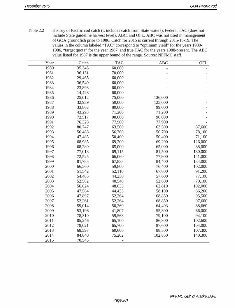
The history of acceptable biological catch (ABC) and total allowable catch (TAC) levels is summarized and compared with the time series of aggregate commercial catches in Table 2.2. For the first year of management under the MFCMA (1977), the catch limit for GOA Pacific cod was established at slightly less than the 1976 total reported landings. During the period 1978-1981, catch limits varied between 34,800 and 70,000 t, settling at 60,000 t in 1982. Prior to 1981 these limits were assigned for “fishing years” rather than calendar years. In 1981 the catch limit was raised temporarily to 70,000 t and the fishing year was extended until December 31 to allow for a smooth transition to management based on calendar years, after which the catch limit returned to 60,000 t until 1986, when ABC began to be set on an annual basis. From 1986 (the first year in which an ABC was set) through 1996, TAC averaged about 83% of ABC and catch averaged about 81% of TAC. In 8 of those 11 years, TAC equaled ABC exactly. In 2 of those 11 years (1992 and 1996), catch exceeded TAC.
To understand the relationships between ABC, TAC, and catch for the period since 1997, it is important to understand that a substantial fishery for Pacific cod has been conducted during these years inside State of Alaska waters, mostly in the Western and Central Regulatory Areas. To accommodate the State-managed fishery, the Federal TAC was set well below ABC (15-25% lower) in each of those years. Thus, although total (Federal plus State) catch has exceeded the Federal TAC in all but three years since 1997, this is basically an artifact of the bi-jurisdictional nature of the fishery and is not evidence of overfishing. At no time since the separate State waters fishery began in 1997 has total catch exceeded ABC, and total catch has never exceeded OFL.
Changes in ABC over time are typically attributable to three factors: 1) changes in resource abundance, 2) changes in management strategy, and 3) changes in the stock assessment model. Assessments conducted prior to 1988 were based on survey biomass alone. From 1988-1993, the assessment was based on stock reduction analysis (Kimura et al. 1984). From 1994-2004, the assessment was conducted using the Stock Synthesis 1 modeling software (Methot 1986, 1990) with length-based data. The assessment was migrated to Stock Synthesis 2 (SS2) in 2005 (Methot 2005b), at which time age-based data began to enter the assessment. Several changes have been made to the model within the SS2 framework (renamed “Stock Synthesis,” or SS3, in 2008) each year since then.
Historically, the majority of the GOA catch has come from the Central regulatory area. To some extent the distribution of effort within the GOA is driven by regulation, as catch limits within this region have been apportioned by area throughout the history of management under the MFCMA. Changes in area-specific allocation between years have usually been traceable to changes in biomass distributions estimated by Alaska Fisheries Science Center trawl surveys or management responses to local concerns. Currently the area-specific ABC allocation is derived from the random effects model (which is similar to the Kalman filter approach). The complete history of allocation (in percentage terms) by regulatory area within the GOA is shown in Table 2.3.
The catches shown in Tables 2.1 and 2.2 include estimated discards (Table 2.4).
In addition to area allocations, GOA Pacific cod is also allocated on the basis of processor component (inshore/offshore) and season. The inshore component is allocated 90% of the TAC and the remainder is allocated to the offshore component. Within the Central and Western Regulatory Areas, 60% of each component’s portion of the TAC is allocated to the A season (January 1 through June 10) and the remainder is allocated to the B season (June 11 through December 31, although the B season directed fishery does not open until September 1).
NMFS has also published the following rule to implement Amendment 83 to the GOA Groundfish FMP:
“Amendment 83 allocates the Pacific cod TAC in the Western and Central regulatory areas of the GOA among various gear and operational sectors, and eliminates inshore and offshore allocations in these two regulatory areas. These allocations apply to both annual and seasonal limits of Pacific cod for the applicable sectors. These apportionments are discussed in detail in a subsequent section of this rule. Amendment 83 is intended to reduce competition among sectors and to support stability in the Pacific cod fishery. The final rule implementing Amendment 83 limits access to the Federal Pacific cod TAC fisheries prosecuted in State of Alaska (State) waters adjacent to the Western and Central regulatory areas in the GOA, otherwise known as parallel fisheries. Amendment 83 does not change the existing annual Pacific cod TAC allocation between the inshore and offshore processing components in the Eastern regulatory area of the GOA.
“In the Central GOA, NMFS must allocate the Pacific cod TAC between vessels using jig gear, catcher vessels (CVs) less than 50 feet (15.24 meters) length overall using hook-and-line gear, CVs equal to or greater than 50 feet (15.24 meters) length overall using hook-and-line gear, catcher/processors (C/Ps) using hook-and-line gear, CVs using trawl gear, C/Ps using trawl gear, and vessels using pot gear. In the Western GOA, NMFS must allocate the Pacific cod TAC between vessels using jig gear, CVs using hook-and-line gear, C/Ps using hook-and-line gear, CVs using trawl gear, and vessels using pot gear. Table 3 lists the proposed amounts of these seasonal allowances. For the Pacific cod sector splits and associated management measures to become effective in the GOA at the beginning of the 2012 fishing year, NMFS published a final rule (76 FR 74670, December 1, 2011) and will revise the final 2012 harvest specifications (76 FR 11111, March 1, 2011).”
“NMFS proposes to calculate of the 2012 and 2013 Pacific cod TAC allocations in the following manner. First, the jig sector would receive 1.5 percent of the annual Pacific cod TAC in the Western GOA and 1.0 percent of the annual Pacific cod TAC in the Central GOA, as required by proposed § 679.20(c)(7). The jig sector annual allocation would further be apportioned between the A (60 percent) and B (40 percent) seasons as required by § 679.20(a)(12)(i). Should the jig sector harvest 90 percent or more of its allocation in a given area during the fishing year, then this allocation would increase by one percent in the subsequent fishing year, up to six percent of the annual TAC. NMFS proposes to allocate the remainder of the annual Pacific cod TAC based on gear type, operation type, and vessel length overall in the Western and Central GOA seasonally as required by proposed § 679.20(a)(12)(A) and (B).”
The longline and trawl fisheries are also associated with a Pacific halibut mortality limit which sometimes constrains the magnitude and timing of harvests taken by these two gear types.
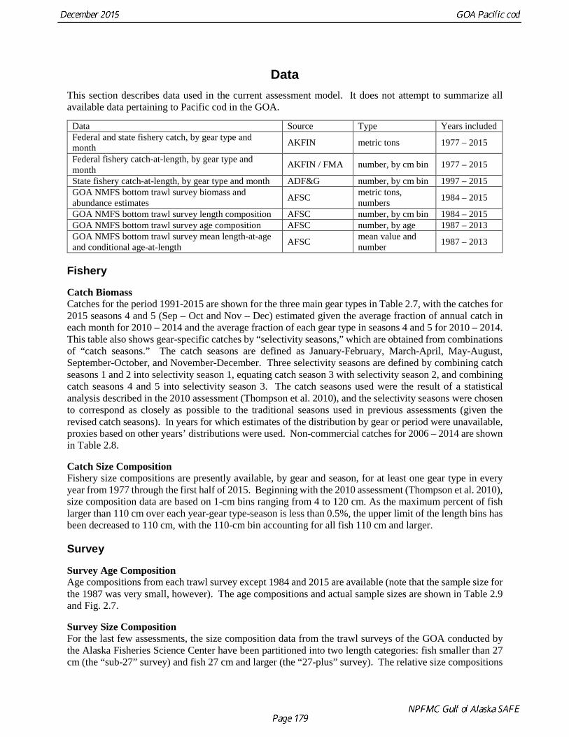
Data This section describes data used in the current assessment model. It does not attempt to summarize all available data pertaining to Pacific cod in the GOA.
Data Source Type Years included Federal and state fishery catch, by gear type and month AKFIN metric tons 1977 – 2015
Federal fishery catch-at-length, by gear type and month AKFIN / FMA number, by cm bin 1977 – 2015
State fishery catch-at-length, by gear type and month ADF&G number, by cm bin 1997 – 2015 GOA NMFS bottom trawl survey biomass and abundance estimates AFSC metric tons,
numbers 1984 – 2015
GOA NMFS bottom trawl survey length composition AFSC number, by cm bin 1984 – 2015 GOA NMFS bottom trawl survey age composition AFSC number, by age 1987 – 2013 GOA NMFS bottom trawl survey mean length-at-age and conditional age-at-length AFSC mean value and
number 1987 – 2013
Fishery
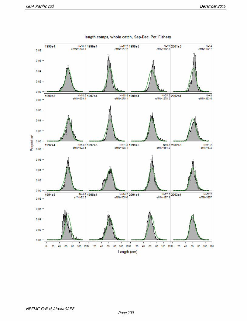
Catch Biomass Catches for the period 1991-2015 are shown for the three main gear types in Table 2.7, with the catches for 2015 seasons 4 and 5 (Sep – Oct and Nov – Dec) estimated given the average fraction of annual catch in each month for 2010 – 2014 and the average fraction of each gear type in seasons 4 and 5 for 2010 – 2014. This table also shows gear-specific catches by “selectivity seasons,” which are obtained from combinations of “catch seasons.” The catch seasons are defined as January-February, March-April, May-August, September-October, and November-December. Three selectivity seasons are defined by combining catch seasons 1 and 2 into selectivity season 1, equating catch season 3 with selectivity season 2, and combining catch seasons 4 and 5 into selectivity season 3. The catch seasons used were the result of a statistical analysis described in the 2010 assessment (Thompson et al. 2010), and the selectivity seasons were chosen to correspond as closely as possible to the traditional seasons used in previous assessments (given the revised catch seasons). In years for which estimates of the distribution by gear or period were unavailable, proxies based on other years’ distributions were used. Non-commercial catches for 2006 – 2014 are shown in Table 2.8.
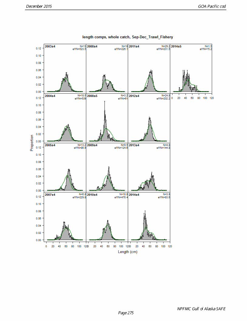
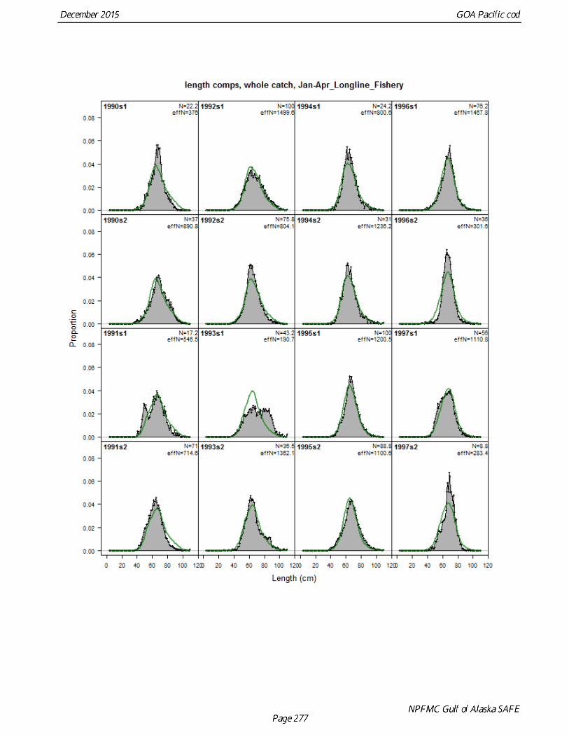
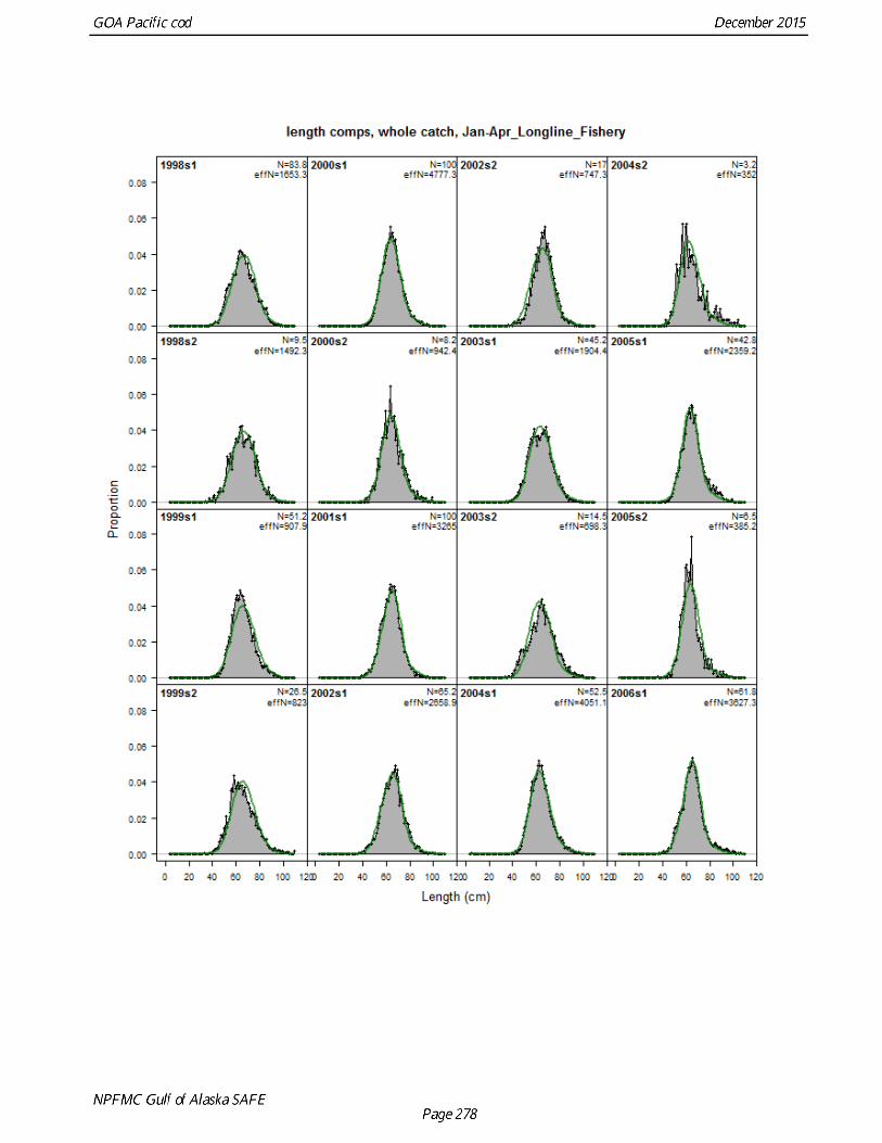
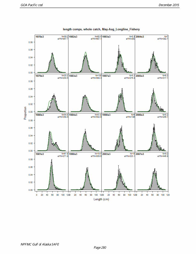
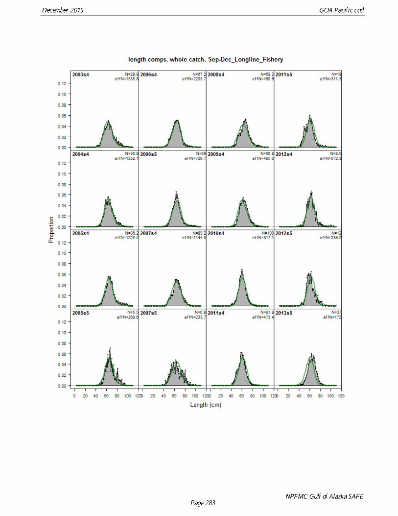
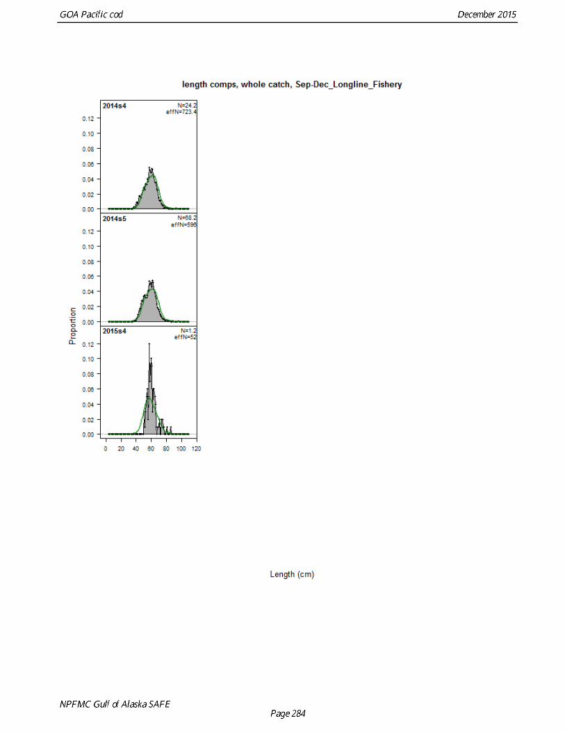
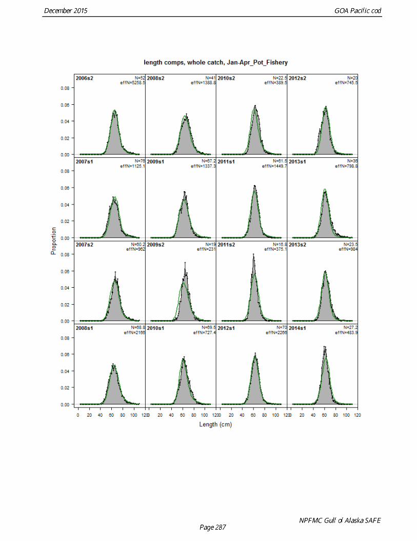
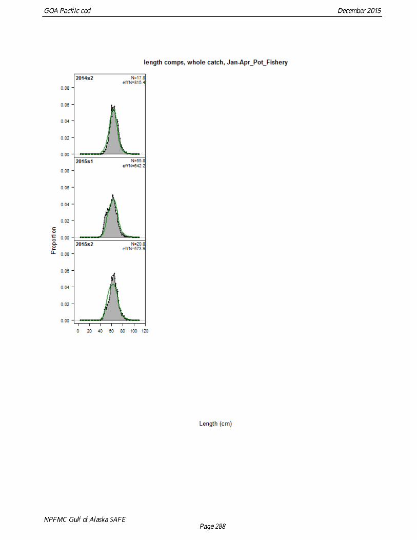
Catch Size Composition Fishery size compositions are presently available, by gear and season, for at least one gear type in every year from 1977 through the first half of 2015. Beginning with the 2010 assessment (Thompson et al. 2010), size composition data are based on 1-cm bins ranging from 4 to 120 cm. As the maximum percent of fish larger than 110 cm over each year-gear type-season is less than 0.5%, the upper limit of the length bins has been decreased to 110 cm, with the 110-cm bin accounting for all fish 110 cm and larger.
Survey
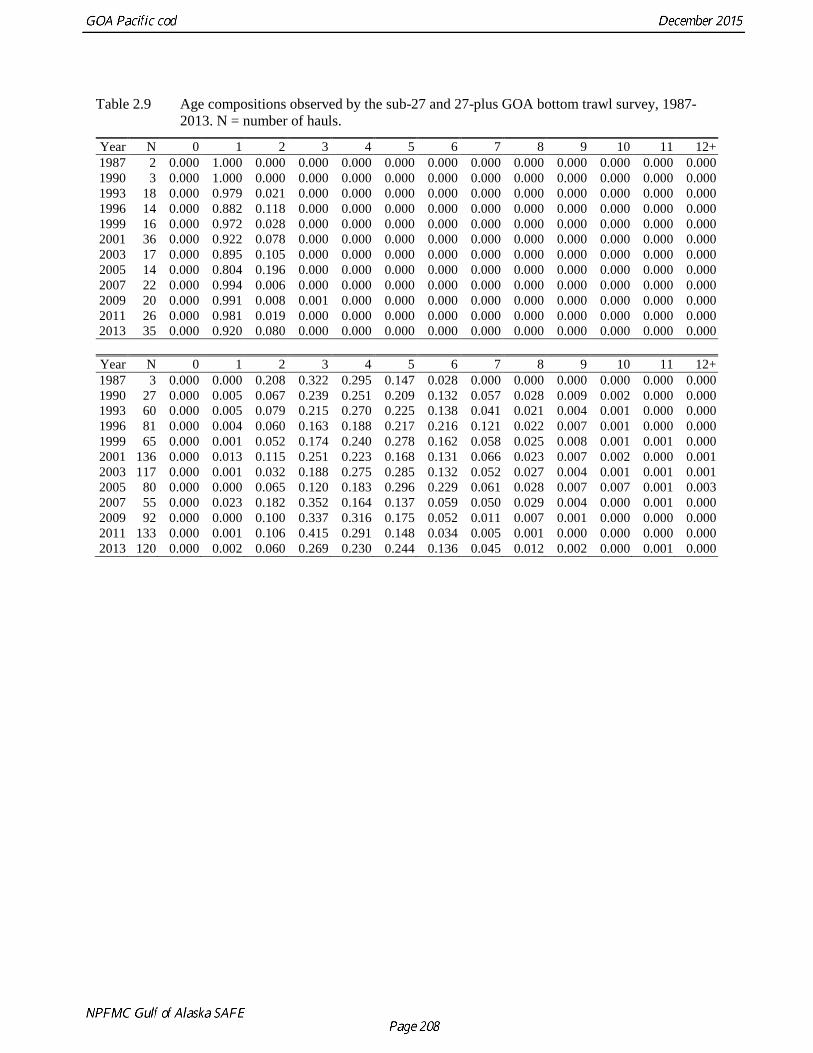
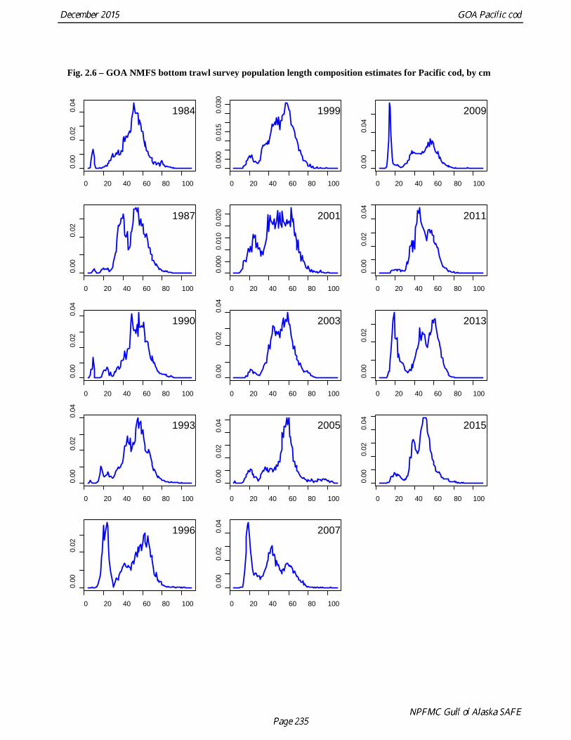
Survey Age Composition Age compositions from each trawl survey except 1984 and 2015 are available (note that the sample size for the 1987 was very small, however). The age compositions and actual sample sizes are shown in Table 2.9 and Fig. 2.7.
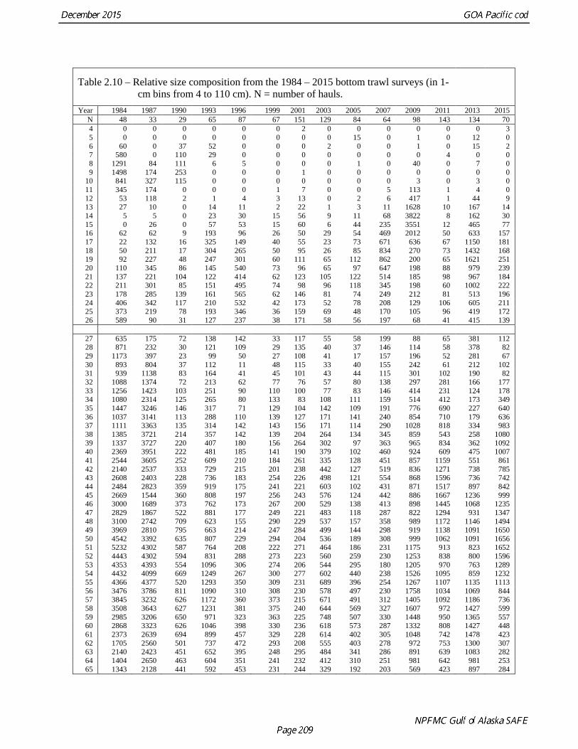
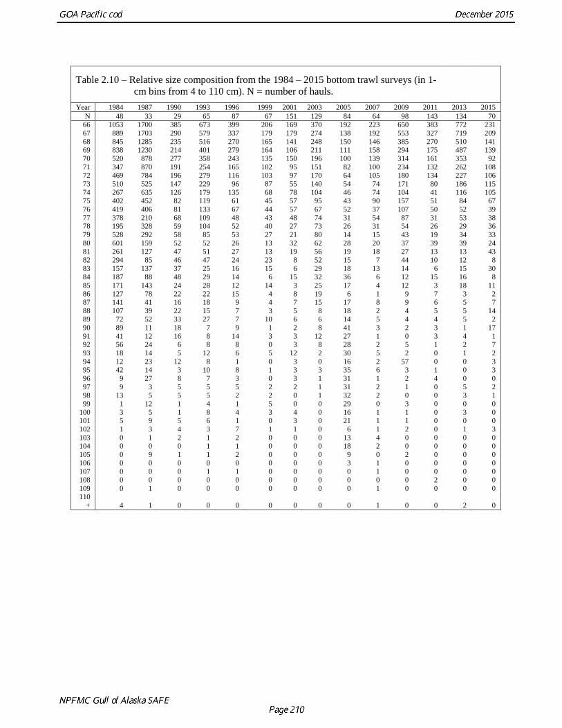
Survey Size Composition For the last few assessments, the size composition data from the trawl surveys of the GOA conducted by the Alaska Fisheries Science Center have been partitioned into two length categories: fish smaller than 27 cm (the “sub-27” survey) and fish 27 cm and larger (the “27-plus” survey). The relative size compositions
from 1984-2015 are shown for the sub-27 and the 27-plus survey in Table 2.10, using the same 1-cm length bins defined above for the fishery catch size compositions. Columns in this table sum to the actual number of fish measured in each year. The full size compositions are shown in Fig. 2.6.
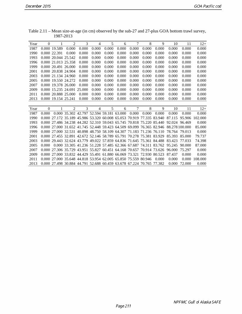
Mean Size at Age Mean size-at-age data are available for all of the years in which age compositions are available. These are shown in Table 2.11.
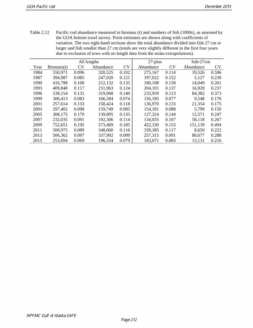
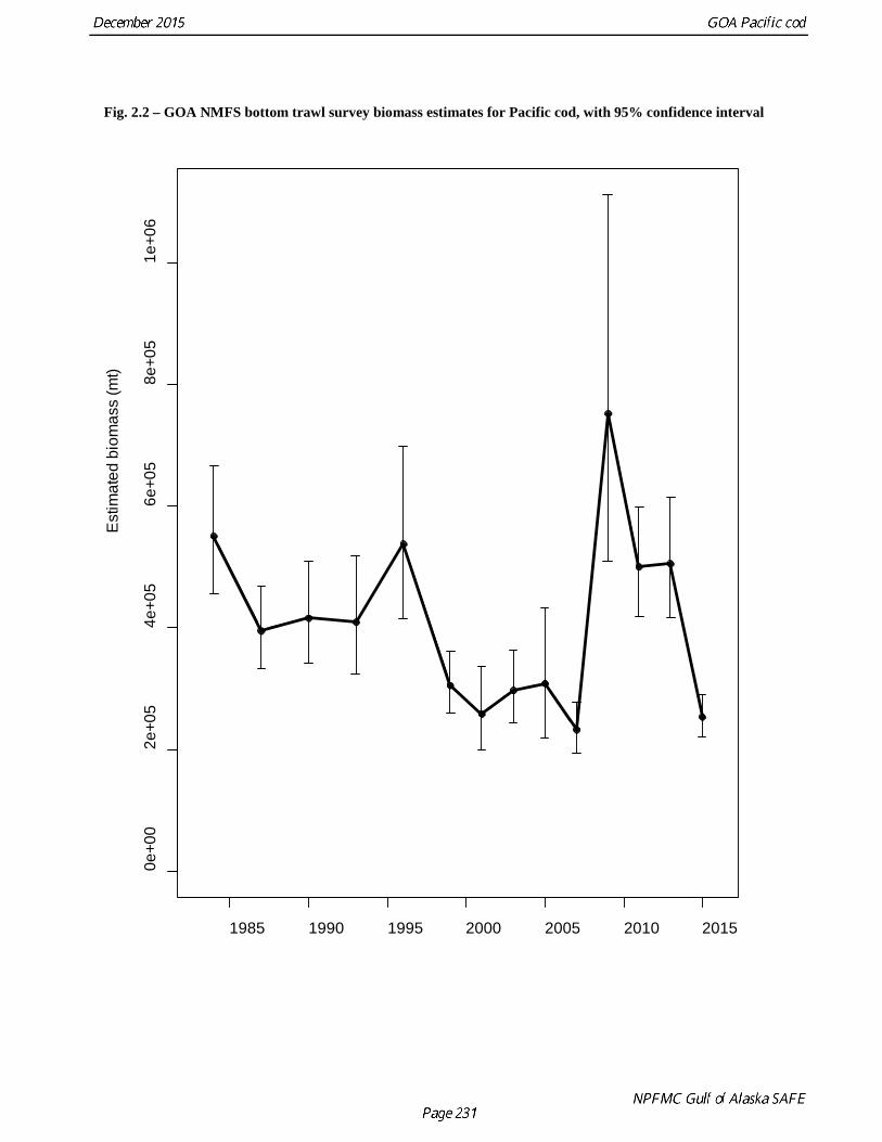
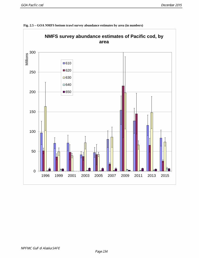
Abundance Estimates Estimates of total abundance (both in biomass and numbers of fish) obtained from the trawl surveys are shown in Table 2.12 and Fig. 2.3, together with their respective coefficients of variation. The abundance estimates by area are shown in Fig. 2.5.
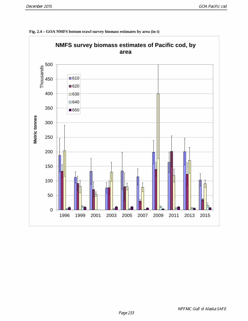
The highest biomass ever observed by the survey was the 2009 estimate of 752,651 t, and the low point was the preceding (2007) estimate of 233,310 t. The 2009 biomass estimate represented a 223% increase over the 2007 estimate. The 2011 biomass estimate was down 33% from 2009, but still 115% above the 2007 estimate. The 2015 biomass estimate is a significant decrease (50%) from the 2013 estimate (Fig. 2.2). The biomass estimates by area are shown in Fig. 2.4.
In terms of population numbers, the record high was observed in 2009, when the population estimated by the survey included over 573 million fish. The 2005 estimate of 140 million fish was the low point in the time series. The 2009 abundance estimate represented a 199% increase over the 2007 estimate. The 2011 abundance estimate was a decrease of 39% from 2009, but still 81% above the 2007 estimate.
The 2015 total abundance estimate is a significant decrease (42%) from the 2013 estimate. The 2015 abundance estimate for fish 27 cm and larger is also a significant decrease of (29%) from the 2013 estimate; the 27-plus abundance estimates have been decreasing by at least 19% between survey years since 2009 (Fig. 2.3). The 2015 abundance estimate for fish less than 27 cm is a large decrease (84%) from the 2013 estimate. The total, 27-plus, and sub-27 abundance estimates for 2015 are a decrease of at least 56% from the 2009 estimates.
Analytic Approach
Model Structure History of Previous Model Structures Developed Under Stock Synthesis Beginning with the 1994 SAFE report (Thompson and Zenger 1994), a model using the Stock Synthesis 1 (SS1) assessment program (Methot 1986, 1990, 1998, 2000) and based largely on length-structured data formed the primary analytical tool used to assess the GOA Pacific cod stock.
SS1 was a program that used the parameters of a set of equations governing the assumed dynamics of the stock (the “model parameters”) as surrogates for the parameters of statistical distributions from which the data were assumed to be drawn (the “distribution parameters”), and varies the model parameters systematically in the direction of increasing likelihood until a maximum is reached. The overall likelihood was the product of the likelihoods for each of the model components. In part because the overall likelihood could be a very small number, SS1 used the logarithm of the likelihood as the objective function. Each likelihood component was associated with a set of data assumed to be drawn from statistical distributions of the same general form (e.g., multinomial, lognormal, etc.). Typically, likelihood components were associated with data sets such as catch size (or age) composition, survey size (or age) composition, and survey abundance (either biomass or numbers, either relative or absolute).
SS1 permitted each data time series to be divided into multiple segments, resulting in a separate set of parameter estimates for each segment. In the base model for the GOA Pacific cod assessment, for example,
possible differences in selectivity between the mostly foreign (also joint venture) and mostly domestic fisheries were accommodated by splitting the fishery size composition time series into pre-1987 and post-1986 segments during the era of SS1-based assessments.
Until 2010, each year was been partitioned into three seasons defined as January-May, June-August, and September-December (these seasonal boundaries were suggested by industry participants in the EBS fishery). Four fisheries were defined during the era of SS1-based assessments: The January-May trawl fishery, the June-December trawl fishery, the longline fishery, and the pot fishery.
Following a series of modifications from 1993 through 1997, the base model for GOA Pacific cod remained completely unchanged from 1997 through 2001. During the late 1990s, a number of attempts were made to estimate the natural mortality rate M and the shelf bottom trawl survey catchability coefficient Q, but these were not particularly successful and the Plan Team and SSC always opted to retain the base model in which M and Q were fixed at traditional values of 0.37 and 1.0, respectively.
A minor modification of the base model was suggested by the SSC in 2001, namely, that consideration be given to dividing the domestic era into pre-2000 and post-1999 segments. This modification was tested in the 2002 assessment (Thompson et al. 2002), where it was found to result in a statistically significant improvement in the model’s ability to fit the data.
A major change took place in the 2005 assessment (Thompson and Dorn 2005), as the model was migrated to the newly developed Stock Synthesis 2 (SS2) program, which made use of the ADMB modeling architecture (Fournier et al. 2012) currently used in most age-structured assessments of BSAI and GOA groundfish. The move to SS2 facilitated improved estimation of model parameters as well as statistical characterization of the uncertainty associated with parameter estimates and derived quantities such as spawning biomass. Technical details of SS2 were described by Methot (2005a, 2007).
The 2006 assessment model (Thompson et al. 2006) was structured similarly to the 2005 assessment model; the primary change being external estimation of growth parameters.
A technical workshop was convened in April, 2007 to consider a wide range of issues pertaining to both the BSAI and GOA Pacific cod assessments (Thompson and Conners 2007).
The 2007 assessment model (Thompson et al. 2007b) for Pacific cod in the GOA was patterned after the model used in that year’s assessment of the BSAI Pacific cod stock (Thompson et al. 2007a), with several changes as described in the assessment document. However, the 2007 assessment model was not accepted by the Plan Team or the SSC.
For the 2008 assessment, the recommended model for the GOA was based largely on the recommended model from the 2008 BSAI Pacific cod assessment. Among other things, this model used an explicit algorithm to determine which fleets (including surveys as well as fisheries) would be forced to exhibit asymptotic selectivity, and another explicit algorithm to determine which selectivity parameters would be allowed to vary periodically in “blocks” of years and to determine the appropriate block length for each such time-varying parameter. One other significant change in the recommended model from the 2008 GOA assessment, which was not shared by the BSAI assessment, was a substantial downweighting of the age composition data. This downweighting was instituted as a means of keeping the root mean squared error of the fit to the survey abundance data close to the sampling variability of those data.
The 2009 assessment (Thompson et al. 2009) featured a total of ten models reflecting a great many alternative assumptions and use or non-use of certain data, particularly age composition data. Relative to the 2008 assessment, the main changes in the model accepted by the Plan Team and SSC were as follow: 1) input standard deviations of all “dev” vectors were set iteratively by matching the standard deviations of the set of estimated “devs;” 2) the standard deviation of length at age was estimated outside the model as a linear function of mean length at age; 3) catchability for the pre-1996 trawl survey was estimated freely
while catchability for the post-1993 trawl survey was fixed at the value that sets the average (weighted by numbers at length) of the product of catchability and selectivity for the 60-81 cm size range equal to the point estimate of 0.916 obtained by Nichol et al. (2007); 4) potential ageing bias was accounted for in the ageing error matrix by examining alternative bias values in increments of 0.1 for ages 2 and above, resulting in a positive bias of 0.4 years for these ages (age-specific bias values were also examined, but did not improve the fit significantly); 5) weighting of the age composition data was returned to its traditional level; 6) except for the parameter governing selectivity at age 0, all parameters of the selectivity function for the post-1993 years of the 27-plus trawl survey were allowed to vary in each survey year except for the most recent; and 7) cohort-specific growth devs were estimated for all years through 2008.
Many changes were made or considered in the 2010 stock assessment model (Thompson et al. 2010). Five models were presented preliminary assessment, as requested by the Plan Teams in May, with subsequent concurrence (given two minor modifications) by the SSC in June. Following review in September and October, three of these models, or modifications thereof, were requested by the Plan Teams or SSC to be included in the final assessment. Relative to the 2009 assessment, the main changes in the model that was ultimately accepted by the Plan Team and SSC in 2010 were as follow: 1) exclude the single record (each) of fishery age composition and mean length-at-age data, 2) use a finer length bin structure than previous models, and 3) re-evaluate the existing seasonal structure used in the model and revise it as appropriate, and 4) remove cohort-specific growth rates (these were introduced for the first time in the 2009 assessment). The new length bin structure consisted of 1-cm bins, replacing the combination of 3-cm and 5-cm bins used in previous assessments. The new seasonal structure consisted of five catch seasons defined as January-February, March-April, May-August, September-October, and November-December; and three selectivity seasons defined as January-April, May-August, and September-December; with spawning identified as occurring at the beginning of the second catch season (March).
Following a review by the Center for Independent Experts in 2011 that resulted in a total of 128 unique recommendations from the three reviewers, the 2011 stock assessment (Thompson et al. 2011) again considered several possible model changes. Three models were requested by the Plan Teams to be included in the final GOA assessment. The SSC concurred, and added one more model. The model that was ultimately accepted by the Team and SSC differed from the 2010 model in the following respects:
• The age corresponding to the L1 parameter in the length-at-age equation was increased from 0 to 1.3333, to correspond to the age of a 1-year-old fish at the time of the survey, which is when the age data are collected. This change was adopted to prevent mean size at age from going negative (as sometimes happened in previous EBS Pacific cod models), and to facilitate comparison of estimated and observed length at age and variability in length at age.
• The parameters governing variability in length at age were re-tuned. This was necessitated by the change in the age corresponding to the L1 parameter (above).
• A column for age 0 fish was added to the age composition and mean-size-at-age portions of the data file. Even though there are virtually no age 0 fish represented in these two portions of the data file, unless a column for age 0 is included, SS will interpret age 1 fish as being ages 0 and 1 combined, which can bias the estimates of year class strength.
• Ageing bias was estimated internally. To preserve a large value for the strength of the 1977 year class and to keep the mean recruitment from the pre-1977 environmental regime lower than the mean recruitment from the post-1976 environmental regime, ageing bias was constrained to be positive (this constraint ultimately proved to be binding only at the maximum age).
It should also be noted that, consistent with Plan Team policy adopted in 2010, quantities that were estimated iteratively in the 2009 assessment were not re-estimated in the 2010 assessment (with the exception of the parameters governing variability in length at age, for the reason listed above).
Model Structures Considered in This Year’s Assessment Stock Synthesis version 3.24S (Methot and Wetzel 2013; Methot 2013) was used to run all the model configurations in this analysis.
One of the models in this year’s assessment are based on the 2014 final model. This model (labeled “Model 0”) is characterized by:
• Three gear types (trawl, longline, and pot), 5 seasons (Jan-Feb, Mar-Apr, May-Aug, Sept-Oct, and Nov-Dec), and three fishery selectivity “seasons” (Jan-Apr, May-Aug, and Sept-Dec);
• Time-varying fishery selectivity-at-length for all gears and seasons (3 – 7 blocks); • Using the GOA NMFS bottom trawl survey as one source of data instead of being split into sub-27
and 27-plus, for the abundance estimates and the length and age composition data; • Using 3 blocks of non-parametric survey selectivity-at-age; • Including the survey conditional age-at-length data; and • Using the recruitment variability multiplier (sigmaR multiplier, value 4.0) for age-0 recruits for
2012, 2013, and 2014.
The model labeled “Model 1” is the 2014 final model with 2015 data, which includes data for the full 2015 GOA NMFS bottom trawl survey.
The additional two models (labeled “Model 2” and “Model 3”) differ significantly from the 2014 final model by:
• Using the 27-plus part of the GOA NMFS bottom trawl survey for the abundance estimates, the length and age composition data, and the conditional age-at-length data;
• Using 4 blocks of non-parametric survey selectivity-at-age; • Increasing Amin from 1 to 3, as data for fish smaller than 27 cm aged 1 and 2 have been omitted; • Capping the sample sizes for the fishery catch-at-length data at 400; and • Evaluating lower weights on the likelihood components for the fishery catch-at-age data
Model 3 differs from Model 2 by including an additional period for fishery selectivity-at-length for 2013 – 2015 for all gear-season combinations except for pot gear season 3, as there were few data for this gear type and season. This selectivity change was made to account for possible changes in the characteristics of the fishery observer length data since the fishery observer program was restructured in 2013.
The author’s preferred model configuration is Model 3, with the weight on the likelihood components for the fishery catch-at-length data decreased from 1 to 0.25.
Parameters Estimated Outside the Assessment Model
Natural Mortality In the 1993 BSAI Pacific cod assessment (Thompson and Methot 1993), the natural mortality rate M was estimated using SS1 at a value of 0.37. All subsequent assessments of the BSAI and GOA Pacific cod stocks (except the 1995 GOA assessment) have used this value for M, until the 2007 assessments, at which time the BSAI assessment adopted a value of 0.34 and the GOA assessment adopted a value of 0.38. Both of these were accepted by the respective Plan Teams and the SSC. The new values were based on Equation 7 of Jensen (1996) and ages at 50% maturity reported by (Stark 2007; see “Maturity” subsection below). In response to a request from the SSC, the 2008 BSAI assessment included further discussion and justification for these values.
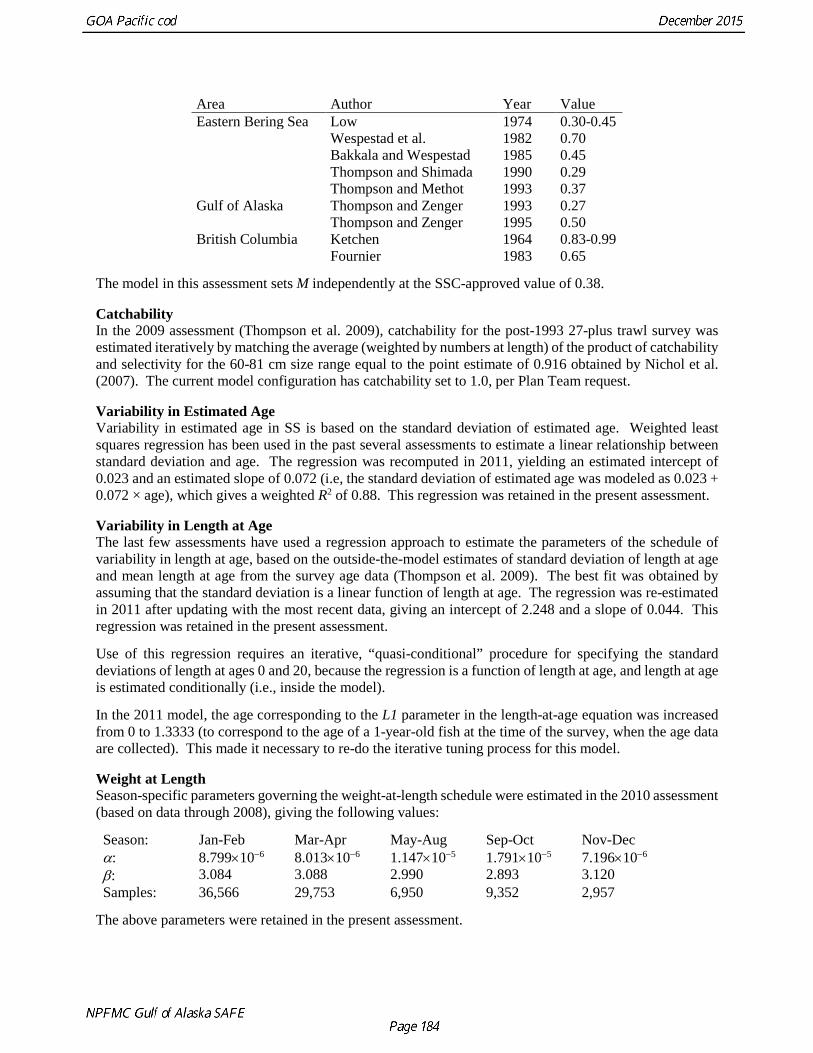
For historical completeness, other published estimates of M for Pacific cod are shown below:
Area Author Year Value Eastern Bering Sea Low 1974 0.30-0.45 Wespestad et al. 1982 0.70 Bakkala and Wespestad 1985 0.45 Thompson and Shimada 1990 0.29 Thompson and Methot 1993 0.37 Gulf of Alaska Thompson and Zenger 1993 0.27 Thompson and Zenger 1995 0.50 British Columbia Ketchen 1964 0.83-0.99 Fournier 1983 0.65
The model in this assessment sets M independently at the SSC-approved value of 0.38.
Catchability In the 2009 assessment (Thompson et al. 2009), catchability for the post-1993 27-plus trawl survey was estimated iteratively by matching the average (weighted by numbers at length) of the product of catchability and selectivity for the 60-81 cm size range equal to the point estimate of 0.916 obtained by Nichol et al. (2007). The current model configuration has catchability set to 1.0, per Plan Team request.
Variability in Estimated Age Variability in estimated age in SS is based on the standard deviation of estimated age. Weighted least squares regression has been used in the past several assessments to estimate a linear relationship between standard deviation and age. The regression was recomputed in 2011, yielding an estimated intercept of 0.023 and an estimated slope of 0.072 (i.e, the standard deviation of estimated age was modeled as 0.023 + 0.072 × age), which gives a weighted R2 of 0.88. This regression was retained in the present assessment.
Variability in Length at Age The last few assessments have used a regression approach to estimate the parameters of the schedule of variability in length at age, based on the outside-the-model estimates of standard deviation of length at age and mean length at age from the survey age data (Thompson et al. 2009). The best fit was obtained by assuming that the standard deviation is a linear function of length at age. The regression was re-estimated in 2011 after updating with the most recent data, giving an intercept of 2.248 and a slope of 0.044. This regression was retained in the present assessment.
Use of this regression requires an iterative, “quasi-conditional” procedure for specifying the standard deviations of length at ages 0 and 20, because the regression is a function of length at age, and length at age is estimated conditionally (i.e., inside the model).
In the 2011 model, the age corresponding to the L1 parameter in the length-at-age equation was increased from 0 to 1.3333 (to correspond to the age of a 1-year-old fish at the time of the survey, when the age data are collected). This made it necessary to re-do the iterative tuning process for this model.
Weight at Length Season-specific parameters governing the weight-at-length schedule were estimated in the 2010 assessment (based on data through 2008), giving the following values:
The above parameters were retained in the present assessment.
Maturity A detailed history and evaluation of parameter values used to describe the maturity schedule for GOA Pacific cod was presented in the 2005 assessment (Thompson and Dorn 2005). A length-based maturity schedule was used for many years. The parameter values used for this schedule in the 2005 and 2006 assessments were set on the basis of a study by Stark (2007) at the following values: length at 50% maturity = 50 cm and slope of linearized logistic equation = −0.222. However, in 2007, changes in SS allowed for use of either a length-based or an age-based maturity schedule. Beginning with the 2007 assessment, the accepted model has used an age-based schedule with intercept = 4.3 years and slope = −1.963 (Stark 2007). The use of an age-based rather than a length-based schedule follows a recommendation from the maturity study’s author (James Stark, ret., Alaska Fisheries Science Center, personal communication). The age-based parameters were retained in the present assessment.
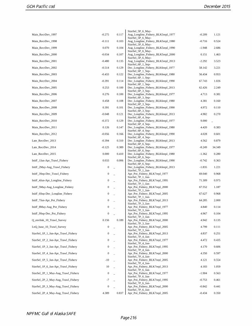
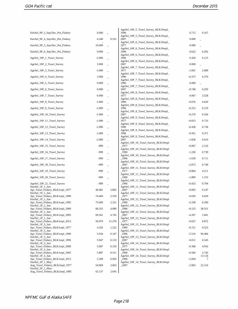
Parameters Estimated Inside the Assessment Model Parameters estimated conditionally (i.e., within individual SS runs, based on the data and the parameters estimated independently) in the model include the von Bertalanffy growth parameters, two ageing bias parameters, log mean recruitment before and since the 1976-1977 regime shift, annual recruitment deviations, initial fishing mortality, gear-season-and-block-specific fishery selectivity parameters, survey selectivity parameters, and pre-1996 catchability for the 27-plus or full survey.
The same functional form (pattern 24 for length-based selectivity, pattern 20 for age-based selectivity) used in Stock Synthesis to define the fishery selectivity schedules in previous year’s assessments was used this year. This functional form, the double normal, is constructed from two underlying and rescaled normal distributions, with a horizontal line segment joining the two peaks. This form uses the following six parameters (selectivity parameters are referenced by these numbers in several of the tables in this assessment):
1. Beginning of peak region (where the curve first reaches a value of 1.0) 2. Width of peak region (where the curve first departs from a value of 1.0) 3. Ascending “width” (equal to twice the variance of the underlying normal distribution) 4. Descending width 5. Initial selectivity (at minimum length/age) 6. Final selectivity (at maximum length/age)
All but the “beginning of peak region” parameter are transformed: The widths are log-transformed and the other parameters are logit-transformed.
Fishery selectivities are length-based and trawl survey selectivities are age-based in these models.
Uniform prior distributions are used for all parameters, except that dev vectors are constrained by input standard deviations (“sigma”), which imply a type of joint prior distribution. These input standard deviations were determined iteratively in the 2009 assessment (Thompson et al. 2009) by matching the standard deviations of the estimated devs. The same input standard deviations were used in this assessment.
For all parameters estimated within individual SS runs, the estimator used is the mode of the logarithm of the joint posterior distribution, which is in turn calculated as the sum of the logarithms of the parameter-specific prior distributions and the logarithm of the likelihood function.
In addition to the above, the full set of year-, season-, and gear-specific fishing mortality rates are also estimated conditionally, but not in the same sense as the above parameters. The fishing mortality rates are determined exactly rather than estimated statistically because SS assumes that the input total catch data are true values rather than estimates, so the fishing mortality rates can be computed algebraically given the other parameter values and the input catch data.
Likelihood Components The model includes likelihood components for trawl survey relative abundance, fishery and survey size composition, survey age composition, survey mean size at age, recruitment, parameter deviations, and “softbounds” (equivalent to an extremely weak prior distribution used to keep parameters from hitting bounds), initial (equilibrium) catch, and survey mean size at age.
In SS, emphasis factors are specified to determine which likelihood components receive the greatest attention during the parameter estimation process. As in previous assessments, all likelihood components were given an emphasis of 1.0 in the present assessment. An evaluation of weights on the fishery catch-at-length likelihood components was performed with Models 2 and 3, as the sum of the fishery catch-at-length likelihood components is over 4 times that of all other likelihood components combined.
Use of Size Composition Data in Parameter Estimation Size composition data are assumed to be drawn from a multinomial distribution specific to a particular year, gear, and season within the year. In the parameter estimation process, SS weights a given size composition observation (i.e., the size frequency distribution observed in a given year, gear, and season) according to the emphasis associated with the respective likelihood component and the sample size specified for the multinomial distribution from which the data are assumed to be drawn. In developing the model upon which SS was originally based, Fournier and Archibald (1982) suggested truncating the multinomial sample size at a value of 400 in order to compensate for contingencies which cause the sampling process to depart from the process that gives rise to the multinomial distribution. For many years, the Pacific cod assessments assumed a multinomial sample size equal to the square root of the true length sample size, rather than the true length sample size itself. Given the true length sample sizes observed in the GOA Pacific cod data, this procedure tended to give values somewhat below 400 while still providing SS with usable information regarding the appropriate effort to devote to fitting individual length samples.
Although the “square root rule” for specifying multinomial sample sizes gave reasonable values, the rule itself was largely ad hoc. In an attempt to move toward a more statistically based specification, the 2007 BSAI assessment (Thompson et al. 2007a) used the harmonic means from a bootstrap analysis of the available fishery length data from 1990-2006. The harmonic means were smaller than the actual sample sizes, but still ranged well into the thousands. A multinomial sample size in the thousands would likely overemphasize the size composition data. As a compromise, the harmonic means were rescaled proportionally in the 2007 BSAI assessment so that the average value (across all samples) was 300. However, the question then remained of what to do about years not covered by the bootstrap analysis (2007 and pre-1990) and what to do about the survey samples. The solution adopted in the 2007 BSAI assessment was based on the consistency of the ratios between the harmonic means (the raw harmonic means, not the rescaled harmonic means) and the actual sample sizes. For the years prior to 1999, the ratio was very consistently close to 0.16, and for the years after 1998, the ratio was very consistently close to 0.34.
This consistency was used to specify input sample sizes for size composition data in all GOA assessments since 2007 as follows: For fishery data, the sample sizes for length compositions from years prior to 1999 were tentatively set at 16% of the actual sample size, and the sample sizes for length compositions from 2007 were tentatively set at 34% of the actual sample size. For the trawl survey, sample sizes were tentatively set at 34% of the actual sample size. Then, all sample sizes were adjusted proportionally so that the average was 300. This method was used to adjust the samples sizes used for the size composition data for analyses performed through 2013.
For the models in this analysis, the number of hauls or trips was used as the sample size instead of the adjusted sample size as calculated above. The sample sizes for the survey length composition data are the number of hauls in that survey year in which cod length frequencies were measured.
The fishery catch-at-length data did not have distinct haul or trip identifiers for all samples, so the adjusted sample size for each year, gear type, and season was the total number of samples multiplied by a scaling factor for each gear type and season. The scaling factor was calculated using the federal fishery observer catch-at-length data for 1987 – 2014. The scaling factor is the ratio of total number of hauls or trips to the total number of samples for each gear type and season.
The sample sizes for the fishery catch-at-length data were capped at 400, which affected 29 out of the 324 sample sizes. The average of the sample sizes for the fishery catch-at-length data with the cap is 149.
Use of Age Composition Data in Parameter Estimation Like the size composition data, the age composition data are assumed to be drawn from a multinomial distribution specific to a particular gear, year, and season within the year. Input sample sizes for the multinomial distributions were computed by scaling the actual number of otoliths read in each year proportionally such that the average of the input sample sizes was equal to 300. This method was used to adjust the samples sizes used for the age composition data for analyses performed through 2013.
For the models in this analysis, the number of hauls was used as the sample size instead of the adjusted sample size as calculated above. For the model configurations with survey age data used as conditional age-at-length data, the sample sizes for a given year sum to the number of hauls in that year.
To avoid double counting of the same data, all models ignore size composition data from each year in which survey age composition data are available.
The average of the sample sizes for the survey population length composition data is 80, and 81 for the survey population age composition data.
Results
Model Evaluation The 2014 final model, without and with data from 2015, and two additional models are presented. The two new models differed in which and how the survey data were used and the number of periods for time-varying survey selectivity-at-age. The model evaluation criteria included the relative sizes of the likelihood components, and how well the model estimates fit to the survey indices, the survey age composition and conditional age-at-length data, reasonable curves for fishery and survey selectivity, the retrospective pattern, and that the model estimated the variance-covariance matrix.
The 2014 final model, without and with data from 2015, labeled “Model 0” and “Model 1”, respectively, were fit to the same catch, fishery catch-at-length, and full GOA NMFS bottom trawl survey abundance, length and age composition data, and conditional age-at-length data excepting the 2015 data. The 2015 models, labeled “Model 2” and “Model 3”, were fit to survey data from the 27-plus part of the GOA NMFS bottom trawl survey. Both sets of models estimated non-parametric survey selectivity-at-age, with the 2014 models estimating 3 periods (1984 – 1993, 1996 – 2005, and 2007 – 2015) and the 2015 models estimating 4 periods (1984 – 1987, 1990 – 1993, 1996 – 2005, and 2007 – 2015) of survey selectivity.
Comparing and Contrasting the Models
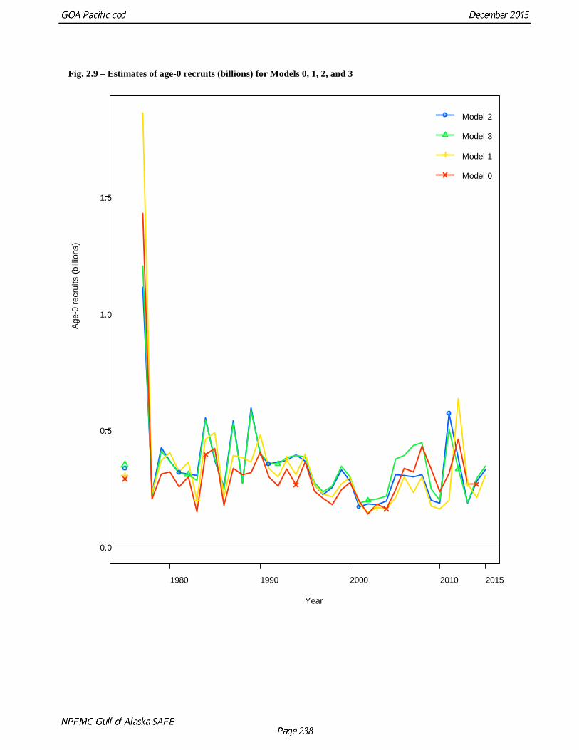
The four models estimated similar patterns for spawning biomass, although the estimates from Model 0 were lower than those from the other models (Fig. 2.8); over the recent period, Models 1 and 2 estimate flat or decreasing spawning biomass, and Models 0 and 3 estimate increasing spawning biomass. The estimates of age-0 recruits differed between the two sets of models for most of the historical period (Fig. 2.9); the differences between Models 0 and 1 were primarily in the recent estimates, as were the estimates for Models 2 and 3. All models fit the survey indices reasonably well in the middle of the time series, and had mediocre fits early and later in the time series, with Models 2 and 3 fitting slightly better to the early abundance estimates than the 2014 models due to the additional early period of survey selectivity (Fig. 2.10); none of the models were able to account well for the large increase in survey abundance between 2007 and 2009, and the significant decreases since 2009.
The two sets of models differed in their fits to their respective sets of survey data with respect to likelihood components (Table 2.13). All models had similar fits to the fishery catch-at-length data. The growth parameter estimates also differed between the two sets of models. The 2015 models, which did not include any survey data for fish less than 27 cm, estimated a higher length-at-Amin and length-at-A∞ than Models 0 and 1; Amin is 1.33333 for Models 0 and 1 and 3.33333 for Models 2 and 3.
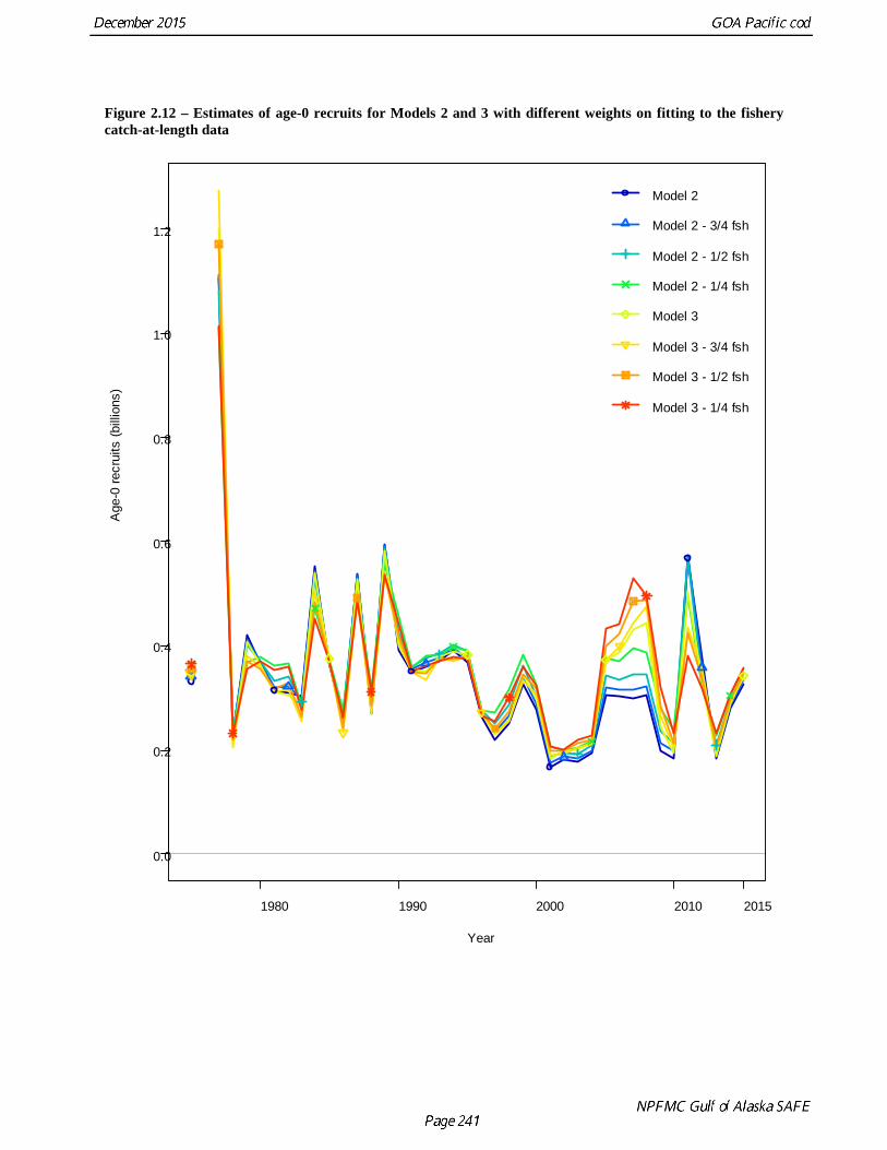
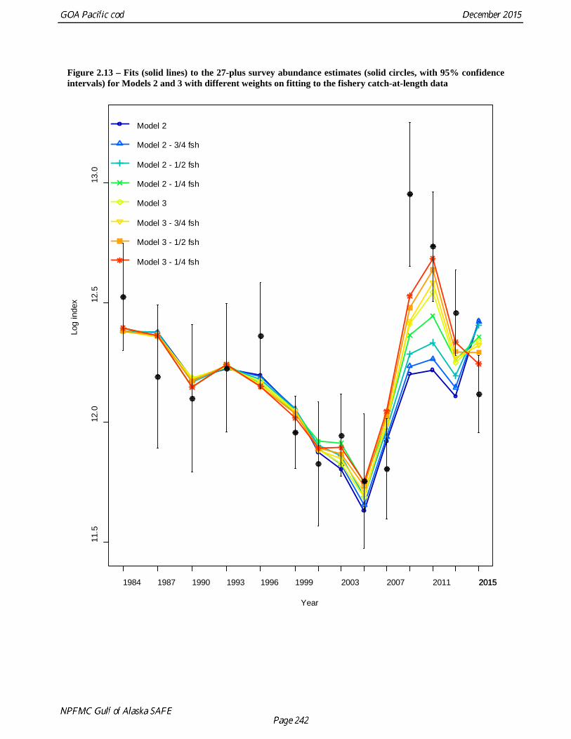
The sum of the likelihood components for the fishery catch-at-length data was over 4 times that of the other likelihood components combined. Different versions of Models 2 and 3 were run with lower weights of ¾, ½, and ¼ applied to the 9 likelihood components for the fishery catch-at-length data to evaluate the impact of the weights on the model fits. These models had the additional designation of “¾ fsh”, “½ fsh”, or “¼ fsh”. All 8 models have similar patterns for spawning biomass (Fig. 2.11), with most of the differences in the recent period, where Model 2 estimated nearly flat values and Model 3 estimated an increase then a decrease. The models with lower weights had lower values for the previously large estimate of 2011 age-0 recruits and higher values for the values from the latter 2000s (Fig. 2.12). The models with lower weights fit to the survey abundance index better than those with higher weights, with Model 3 fitting better than Model 2 (Fig. 2.13).
Evaluation Criteria
Model 3 fit the 27-plus survey data better than Model 2, and fit the fishery catch-at-length data better as well, excepting pot gear seasons 1, 2, and 3. All model configurations had reasonable fishery selectivity-at-length curves. All model configurations converged and produced variance-covariance matrices.
Selection of final model
Models 2 and 3 are preferred over the 2014 models, as the new models omit most of the more variable part of the survey data, the age-1 data. Models 2 and 3 with the weights on the fishery catch-at-length data of ¼ fit the survey data better than the models with higher weights. Model 3, the model with a new period of fishery selectivity for 2013 – 2015, fit the data better than Model 2. The preferred model is Model 3 – ¼ fsh, as this model was best able to estimate the survey abundance index from 2007 through 2015. Model 2 – ¼ fsh could be the alternate preferred model if there does not appear to be enough evidence for a change in the fishery catch-at-length data characteristics since 2013.
Final parameter estimates and associated schedules
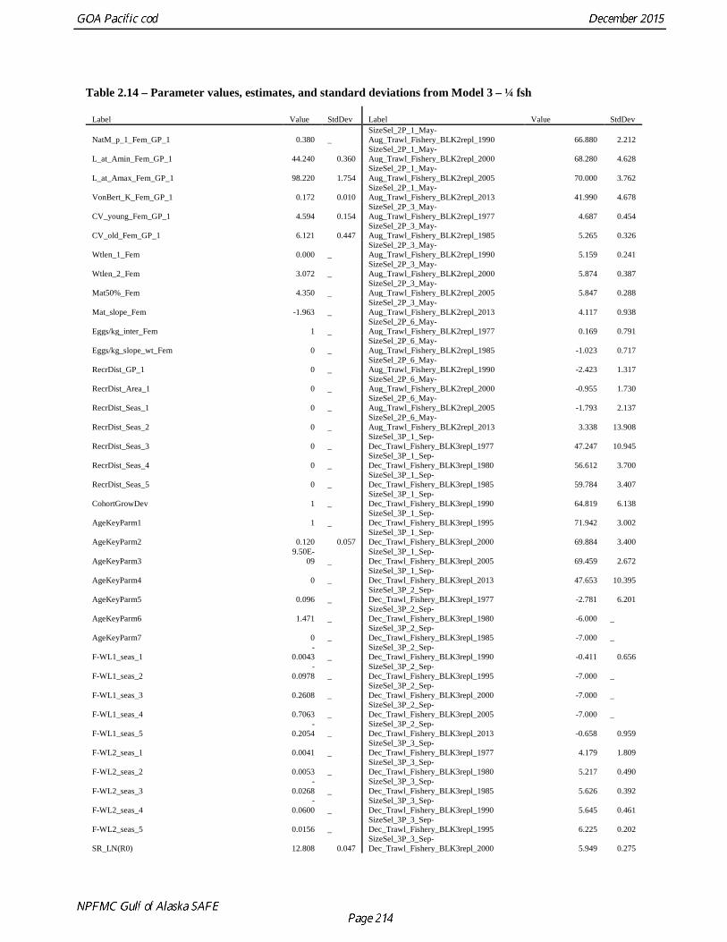
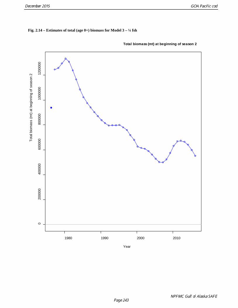
The fixed and estimated parameters for Model 3 – ¼ fsh are listed in Table 2.14. Total biomass has decreased from a peak in 1980 to a low in 2008 and is increasing (Fig. 2.14); spawning biomass has a similar pattern with more uncertainty for the recent years (Fig. 2.15). Age-0 recruits had the highest value at the beginning of the time series and had moderate variability since then (Fig. 2.16). The estimates of the 27-plus survey abundance estimates fit the data reasonably well, and less well in for 2007 and 2009, due to the large difference and the high estimate for 2009 (Fig. 2.17). There does not appear to be a strong
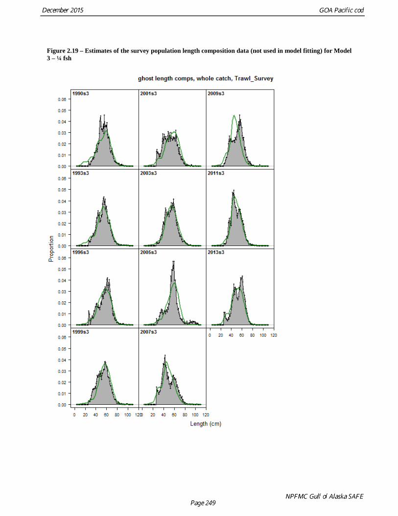
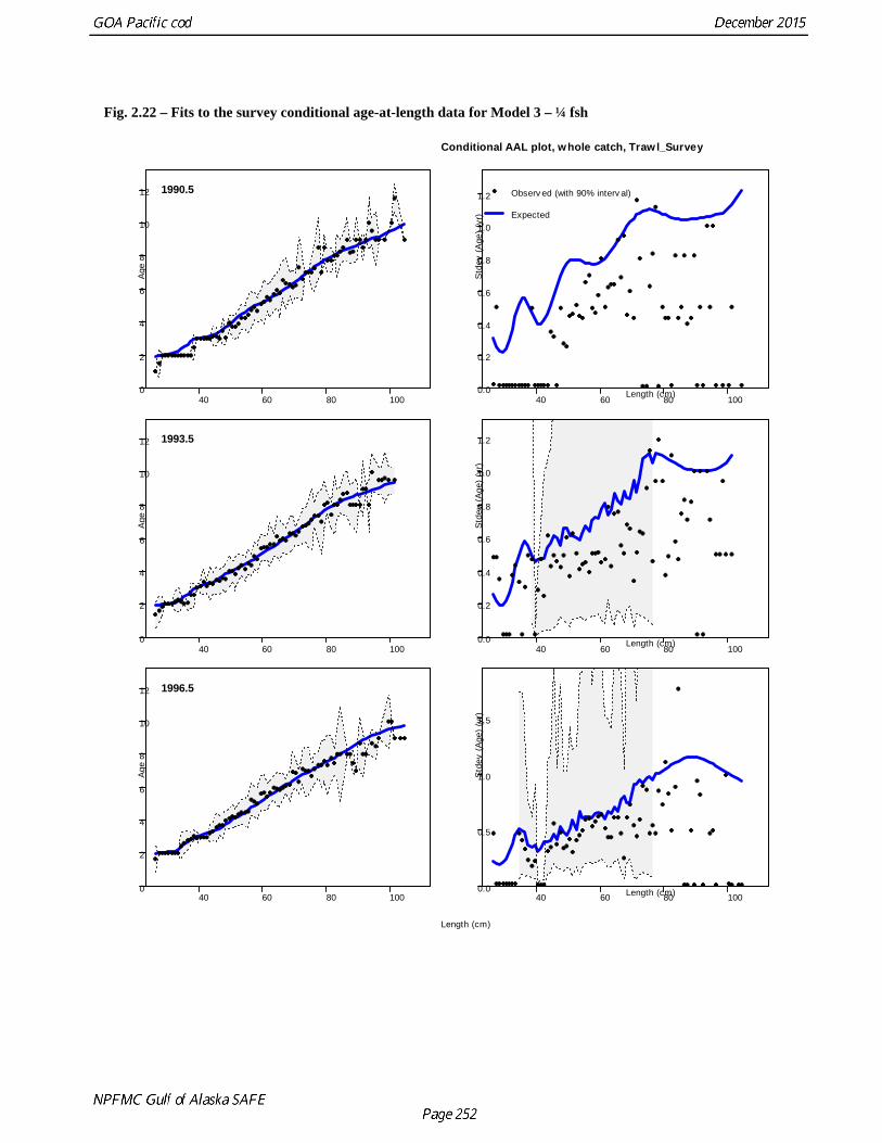
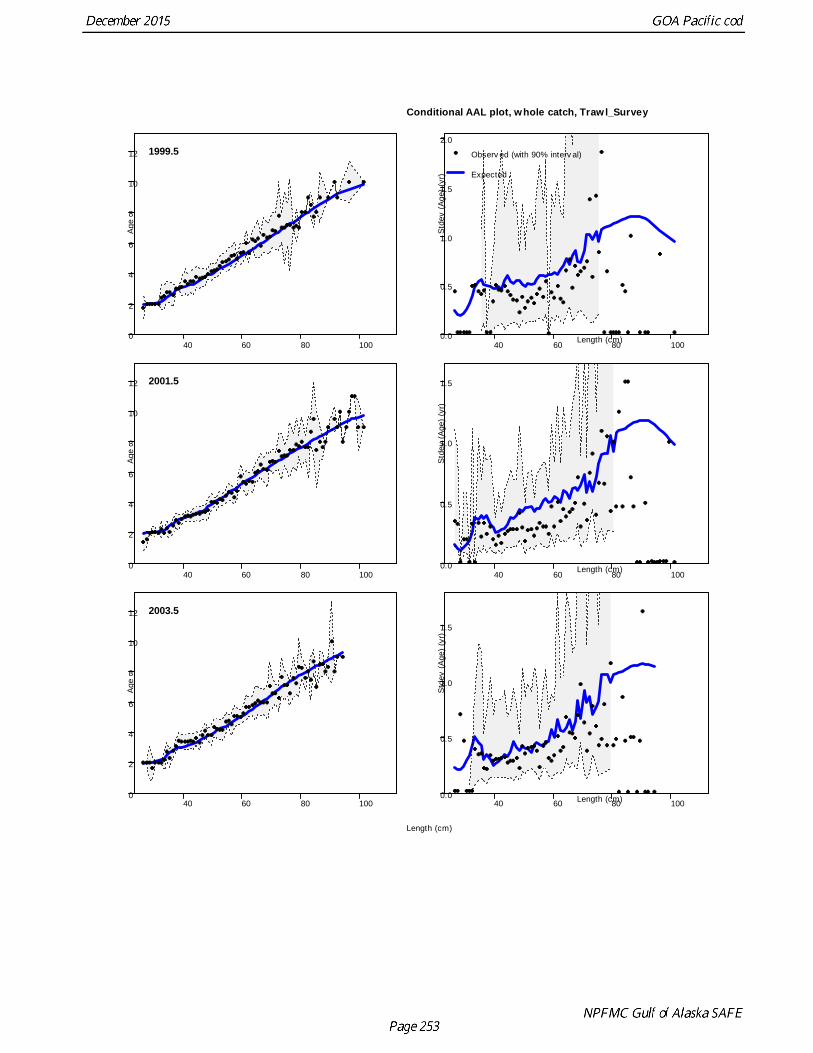
relationship between spawning biomass and recruitment (Fig. 2.18). The estimates of the survey population length composition data are reasonable in most years, with an overestimate of 40-cm fish in 2009 (Fig. 2.19). The fits to the survey population age composition data are reasonable (Fig. 2.20), as are the fits to the survey population length composition data (Fig. 2.21). The fits to the survey conditional age-at-length data are good, with moderate variability where there are abundant data (Fig. 2.22). The estimated length-at-age relationship is shown in Fig. 2.13.
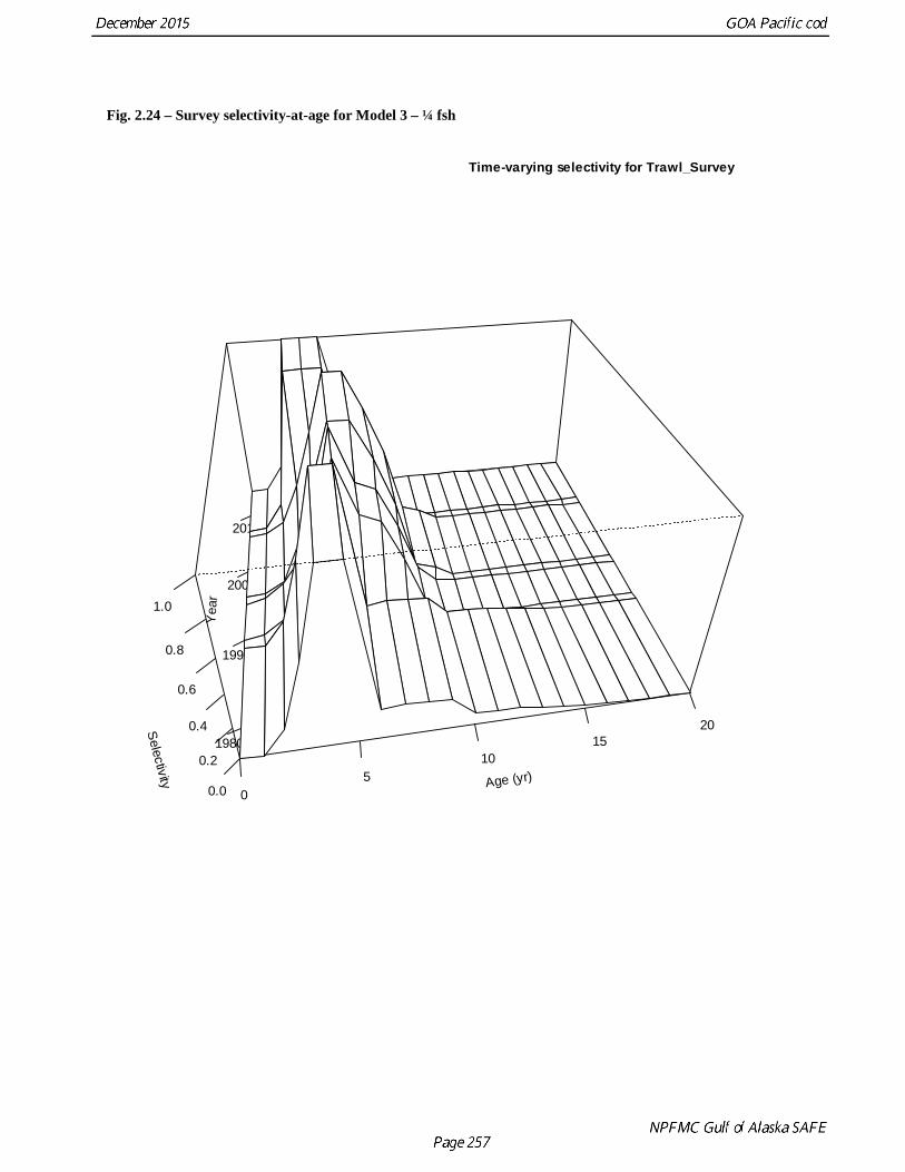
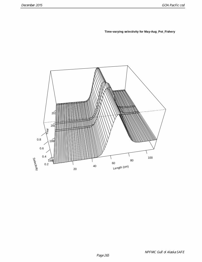
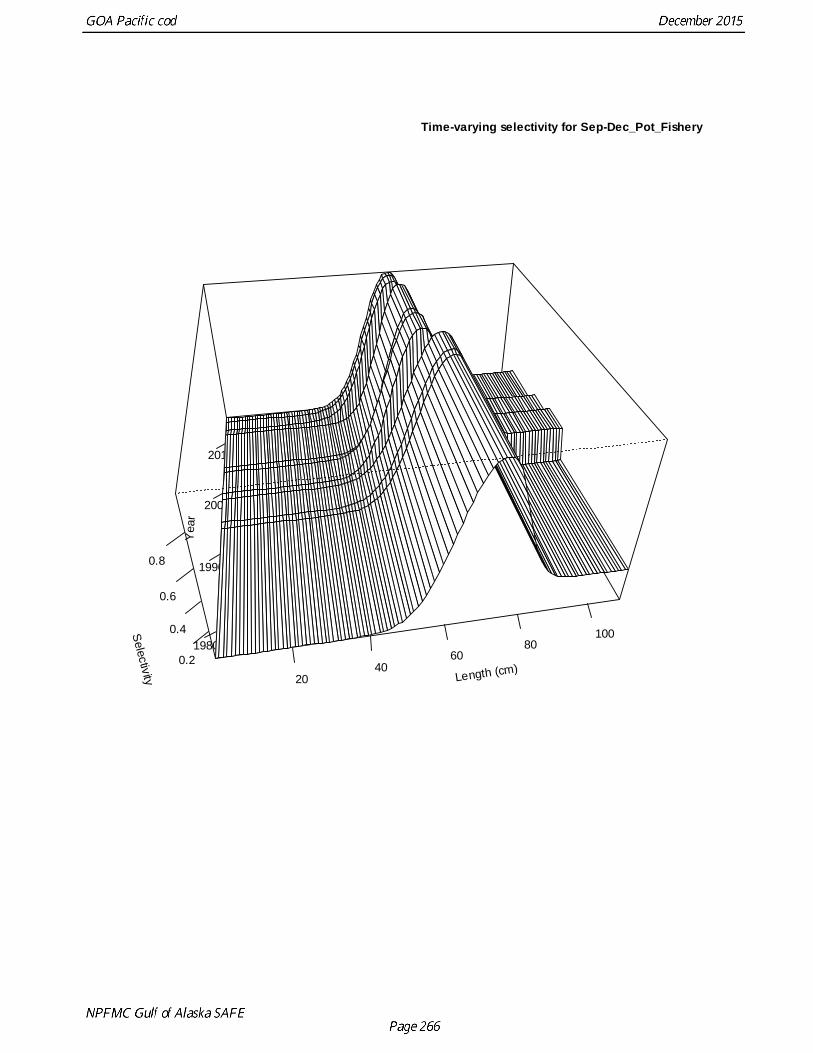
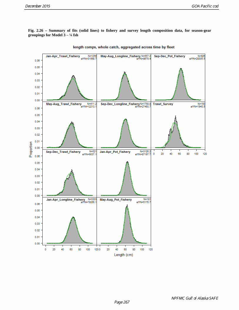
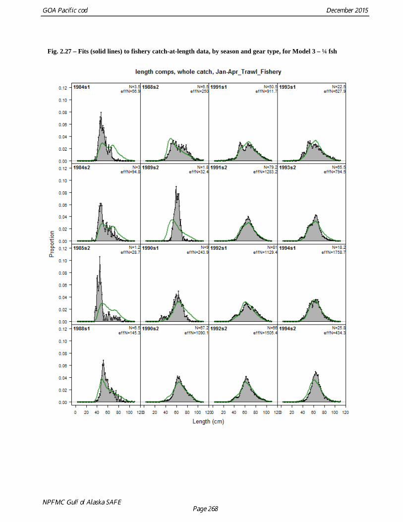
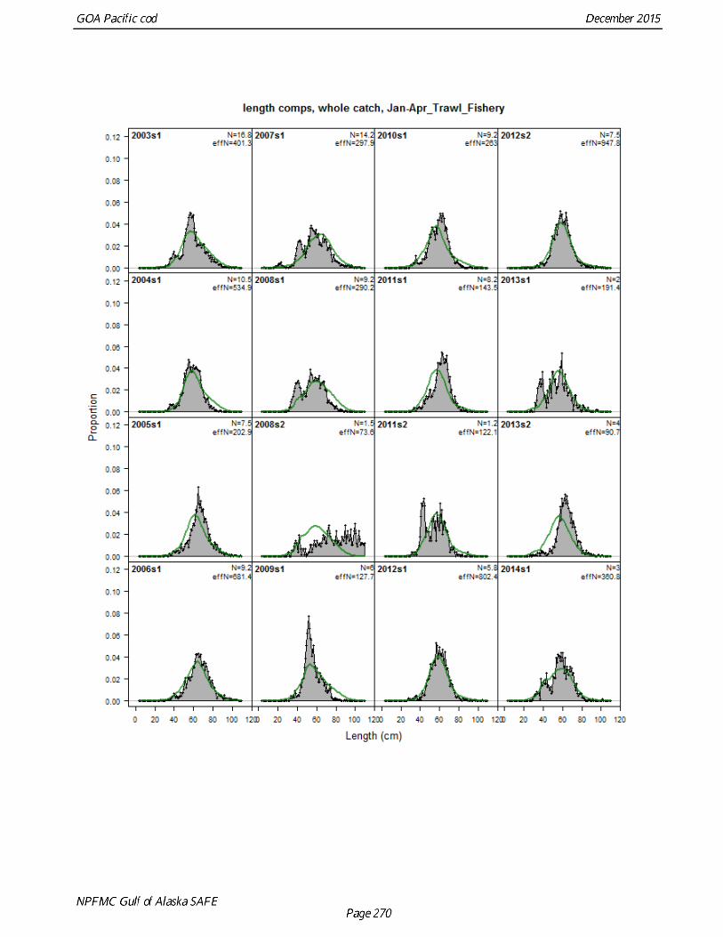
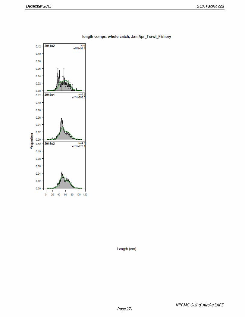
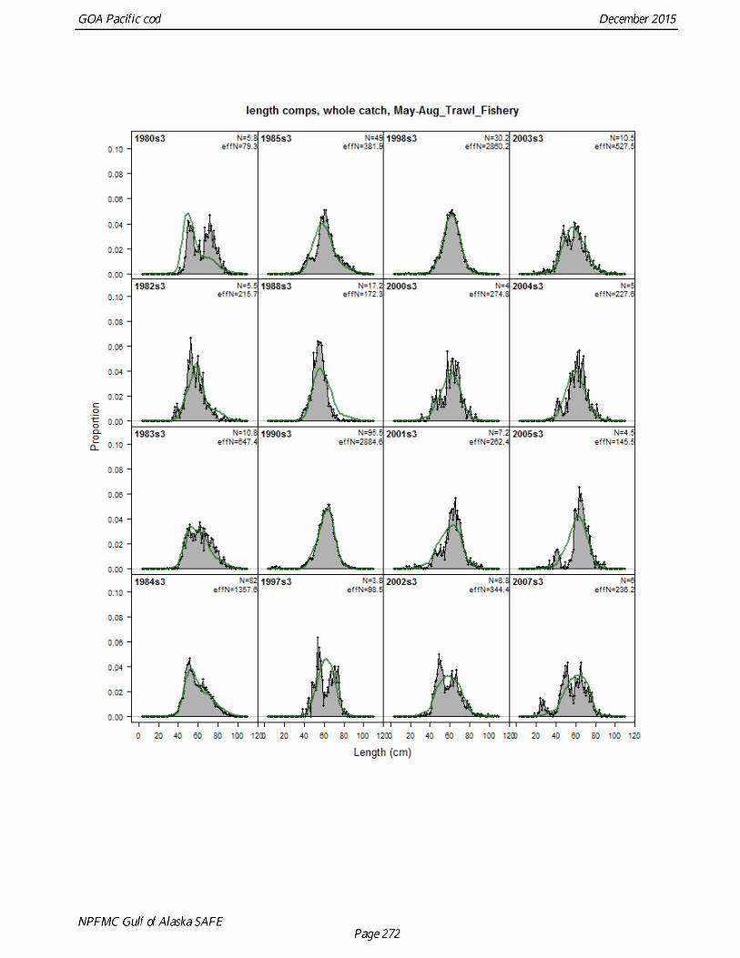
Survey selectivity-at-age for the latter period had a peak at a lower age than the previous period (Fig. 2.24). Fishery selectivity-at-length was more variable, both within and between seasons and gear types, with the new period for 2013 – 2015 estimated to have a lower peak for all seasons and gear types with the new period (Fig. 2.25). The fits to the fishery catch-at-length data were reasonable in most years (Figs. 2.26 and 2.27).
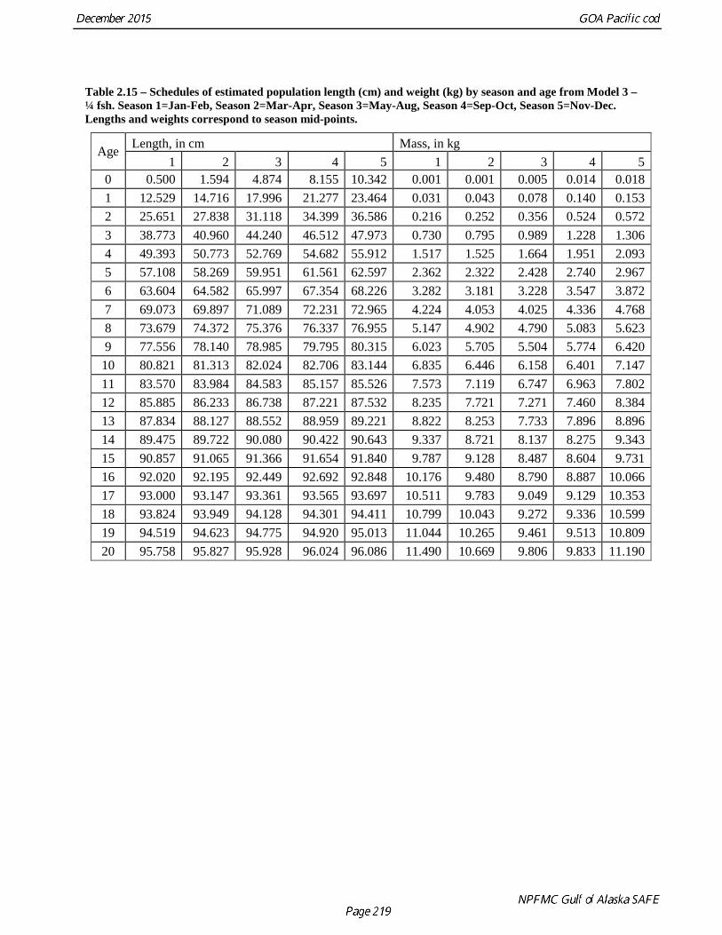
The seasonal length-at-age and weight-at-age schedules are in Table 2.15. Survey selectivity-at-age by time period is in Table 2.16.
Time Series Results
Definitions The biomass estimates presented here will be defined in two ways: 1) age 0+ biomass, consisting of the biomass of all fish aged 0 years or greater in a given year; and 2) spawning biomass, consisting of the biomass of all spawning females in a given year. The recruitment estimates presented here will be defined as numbers of age-0 fish in a given year.
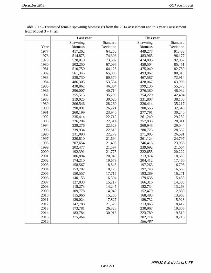
Biomass Table 2.17 shows the time series of GOA Pacific cod female spawning biomass for the years 1977-2015 as estimated last year and this year. The estimated spawning biomass time series are accompanied by their respective standard deviations. Total and spawning biomass are shown in Figs. 2.14 and 2.15.
Recruitment and Numbers at Age Table 2.18 shows the time series of GOA Pacific cod age-0 recruits for the years 1977-2014 as estimated last year and this year. The estimated recruitment time series are accompanied by their respective standard deviations (Fig. 2.16). Table 2.19 shows the numbers-at-age for 1977-2015.
Survey Data Fig. 2.17 shows the fit to the 27-plus survey abundance estimates. Fig. 2.19 shows the 1990 – 2013 survey length composition data, which were not used in model fitting, and the estimated survey length composition. Fig. 2.20 shows the fit to the survey age composition data and Fig. 2.21 shows the fit to the survey length composition data for 1984, 1987, and 2015. Figure 2.22 shows the fit to the survey conditional age-at-length data.
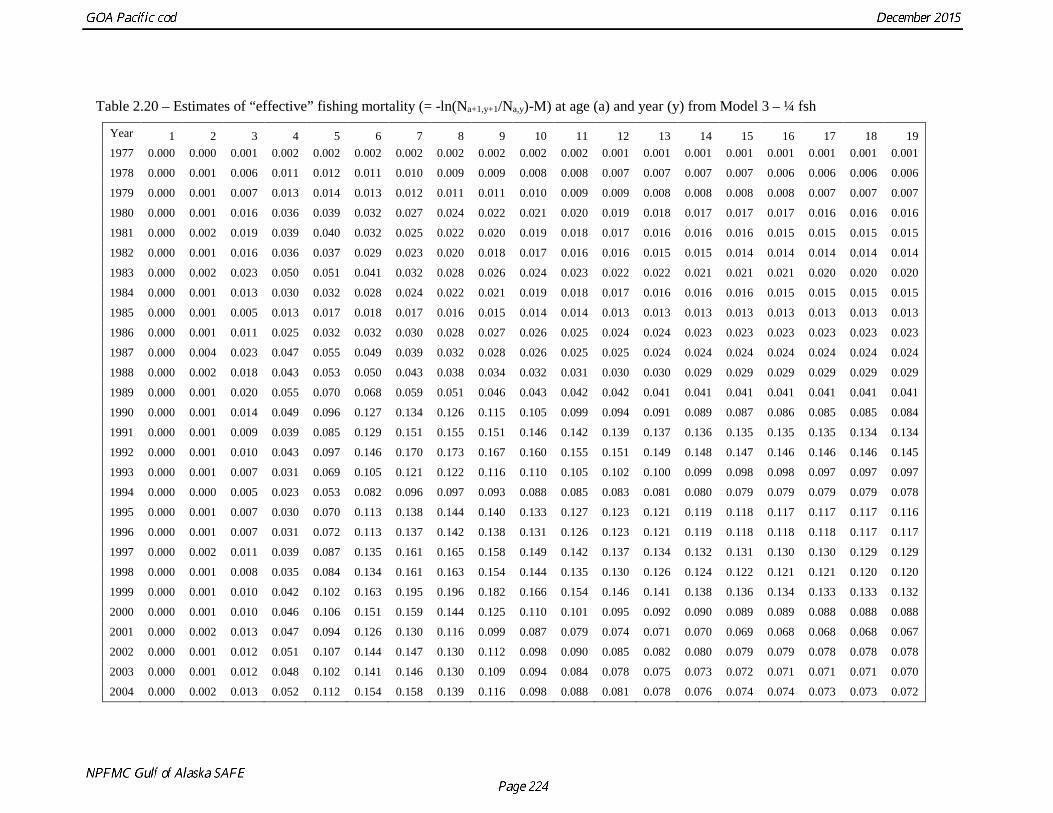
Fishing Mortality Table 2.20 shows the “effective” annual fishing mortality by age and year for ages 1-19 and years 1977-2014. The “effective” annual fishing mortality is -ln(Na+1,y+1/Na,y)-M.
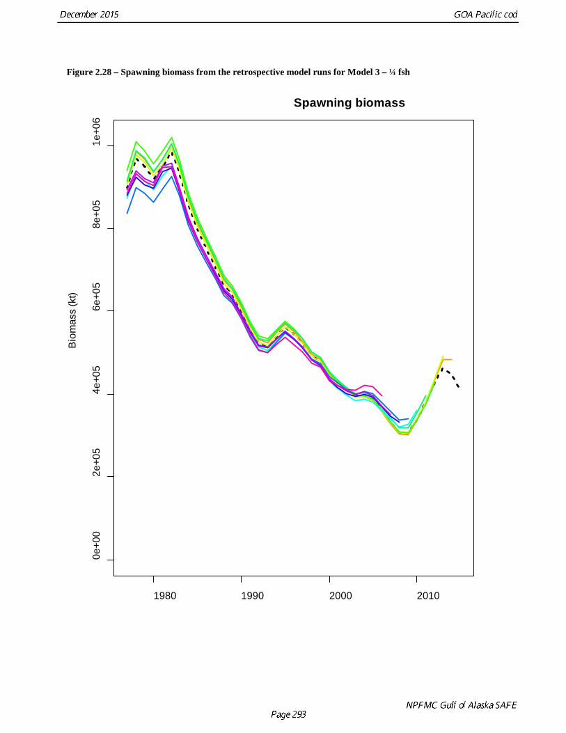
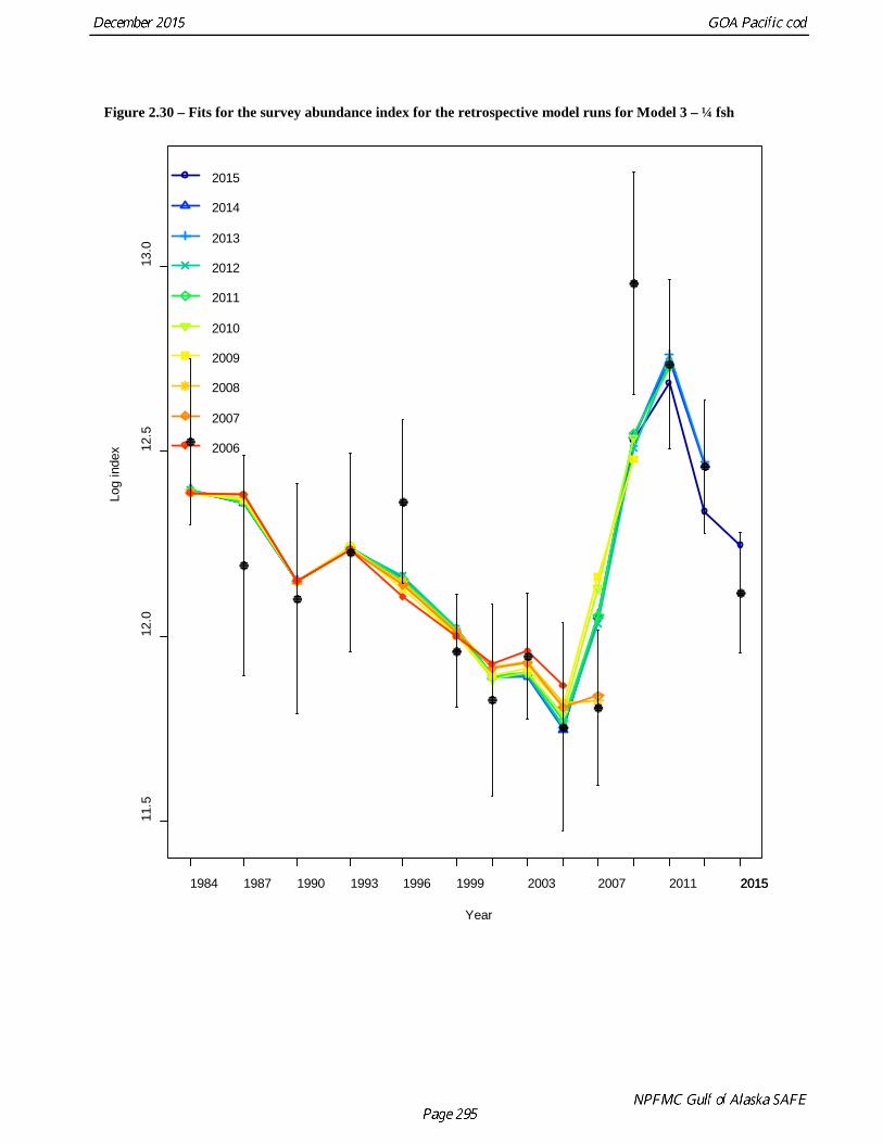
Retrospective analysis Estimates of spawning biomass for Model 3 – ¼ fsh with an ending year of 2006 through 2015 are very similar for 1984 through 2000, and have a consistent downward adjustment for the recent years as more data are included (Fig. 2.28). Relative differences in estimates of spawning biomass show the same pattern for the more recent years (Fig. 2.29). The fits to the survey abundance index were similar for all years, with more difference for the recent estimates for 2015 and the earlier years (Fig. 2.30).
Harvest Recommendations Amendment 56 Reference Points Amendment 56 to the GOA Groundfish Fishery Management Plan (FMP) defines the “overfishing level” (OFL), the fishing mortality rate used to set OFL (FOFL), the maximum permissible ABC, and the fishing mortality rate used to set the maximum permissible ABC. The fishing mortality rate used to set ABC (FABC) may be less than this maximum permissible level, but not greater. Because reliable estimates of reference points related to maximum sustainable yield (MSY) are currently not available but reliable estimates of reference points related to spawning per recruit are available, Pacific cod in the GOA have generally been managed under Tier 3 of Amendment 56. Tier 3 uses the following reference points: B40%, equal to 40% of the equilibrium spawning biomass that would be obtained in the absence of fishing; F35%, equal to the fishing mortality rate that reduces the equilibrium level of spawning per recruit to 35% of the level that would be obtained in the absence of fishing; and F40%, equal to the fishing mortality rate that reduces the equilibrium level of spawning per recruit to 40% of the level that would be obtained in the absence of fishing. The following formulae apply under Tier 3:
Other useful biomass reference points which can be calculated using this assumption are B100% and B35%, defined analogously to B40%. These reference points are estimated as follows, based on this year’s model, Model 3 – ¼ fsh:
Reference point: B35% B40% B100% Spawning biomass: 113,800 t 130,000 t 325,200 t
For a stock exploited by multiple gear types, estimation of F35% and F40% requires an assumption regarding the apportionment of fishing mortality among those gear types. For this assessment, the apportionment was based on this year’s model’s estimates of fishing mortality by gear for the five most recent complete years of data (2010-2014). The average fishing mortality rates for those years implied that total fishing mortality was divided among the three main gear types according to the following percentages: trawl 20.5%, longline 22.4%, and pot 57.1%. This apportionment results in estimates of F35% and F40% equal to 0.495 and 0.407, respectively.
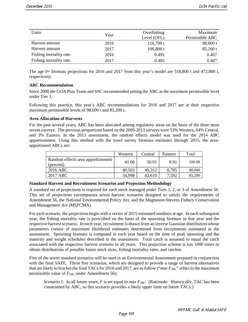
Specification of OFL and Maximum Permissible ABC Spawning biomass for 2016 is estimated by this year’s model to be 165,600 t. This is above the B40% value of 130,000 t, thereby placing Pacific cod in sub-tier “a” of Tier 3. Given this, the model estimates OFL, maximum permissible ABC, and the associated fishing mortality rates for 2016 and 2017 as follows (2017 values are predicated on the assumption that 2016 catch will equal 2016 maximum permissible ABC):
Units Year Overfishing Level (OFL)
Maximum Permissible ABC
Harvest amount 2016 116,700 t 98,600 t Harvest amount 2017 100,800 t 85,200 t Fishing mortality rate 2016 0.495 0.407 Fishing mortality rate 2017 0.495 0.407
The age 0+ biomass projections for 2016 and 2017 from this year’s model are 518,800 t and 472,800 t, respectively.
ABC Recommendation Since 2008 the GOA Plan Team and SSC recommended setting the ABC at the maximum permissible level under Tier 3.
Following this practice, this year’s ABC recommendations for 2016 and 2017 are at their respective maximum permissible levels of 98,600 t and 85,200 t.
Area Allocation of Harvests For the past several years, ABC has been allocated among regulatory areas on the basis of the three most recent surveys. The previous proportions based on the 2009-2013 surveys were 33% Western, 64% Central, and 3% Eastern. In the 2013 assessment, the random effects model was used for the 2014 ABC apportionment. Using this method with the trawl survey biomass estimates through 2015, the area-apportioned ABCs are:
Western Central Eastern Total Random effects area apportionment (percent) 41.08 50.01 8.91 100.00
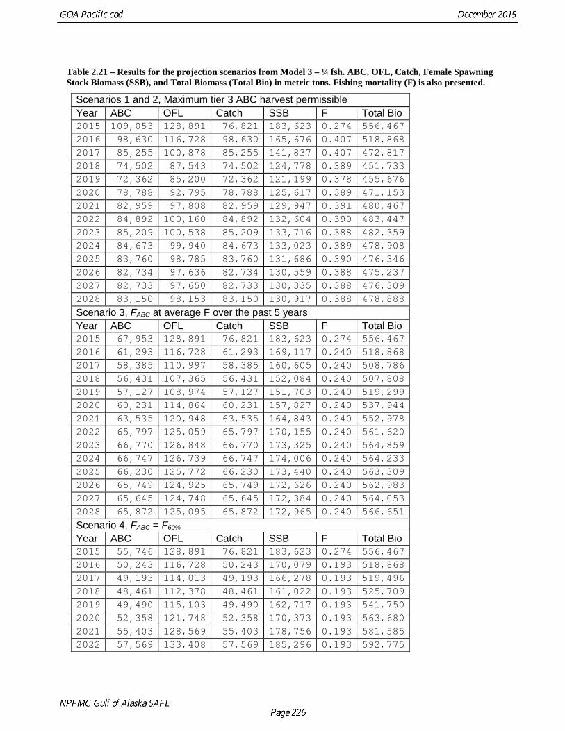
Standard Harvest and Recruitment Scenarios and Projection Methodology A standard set of projections is required for each stock managed under Tiers 1, 2, or 3 of Amendment 56. This set of projections encompasses seven harvest scenarios designed to satisfy the requirements of Amendment 56, the National Environmental Policy Act, and the Magnuson-Stevens Fishery Conservation and Management Act (MSFCMA).
For each scenario, the projections begin with a vector of 2015 estimated numbers at age. In each subsequent year, the fishing mortality rate is prescribed on the basis of the spawning biomass in that year and the respective harvest scenario. In each year, recruitment is drawn from an inverse Gaussian distribution whose parameters consist of maximum likelihood estimates determined from recruitments estimated in the assessment. Spawning biomass is computed in each year based on the time of peak spawning and the maturity and weight schedules described in the assessment. Total catch is assumed to equal the catch associated with the respective harvest scenario in all years. This projection scheme is run 1000 times to obtain distributions of possible future stock sizes, fishing mortality rates, and catches.
Five of the seven standard scenarios will be used in an Environmental Assessment prepared in conjunction with the final SAFE. These five scenarios, which are designed to provide a range of harvest alternatives that are likely to bracket the final TACs for 2016 and 2017, are as follow (“max FABC” refers to the maximum permissible value of FABC under Amendment 56):
Scenario 1: In all future years, F is set equal to max FABC. (Rationale: Historically, TAC has been constrained by ABC, so this scenario provides a likely upper limit on future TACs.)
Scenario 2: In all future years, F is set equal to a constant fraction of max FABC, where this fraction is equal to the ratio of the FABC value for 2016 recommended in the assessment to the max FABC for 2016. (Rationale: When FABC is set at a value below max FABC, it is often set at the value recommended in the stock assessment.)
Scenario 3: In all future years, F is set equal to the 2010-2014 average F. (Rationale: For some stocks, TAC can be well below ABC, and recent average F may provide a better indicator of FTAC than FABC.)
Scenario 4: In all future years, the upper bound on FABC is set at F60%. (Rationale: This scenario provides a likely lower bound on FABC that still allows future harvest rates to be adjusted downward when stocks fall below reference levels.)
Scenario 5: In all future years, F is set equal to zero. (Rationale: In extreme cases, TAC may be set at a level close to zero.)
Two other scenarios are needed to satisfy the MSFCMA’s requirement to determine whether a stock is currently in an overfished condition or is approaching an overfished condition. These two scenarios are as follow (for Tier 3 stocks, the MSY level is defined as B35%):
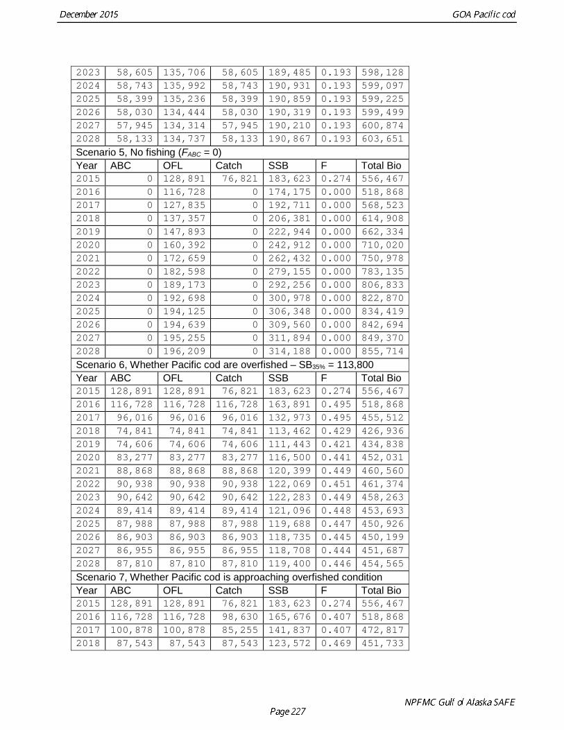
Scenario 6: In all future years, F is set equal to FOFL. (Rationale: This scenario determines whether a stock is overfished. If the stock is 1) above its MSY level in 2015, or 2) above 1/2 of its MSY level in 2015 and expected to be above its MSY level in 2025 under this scenario, then the stock is not overfished.)
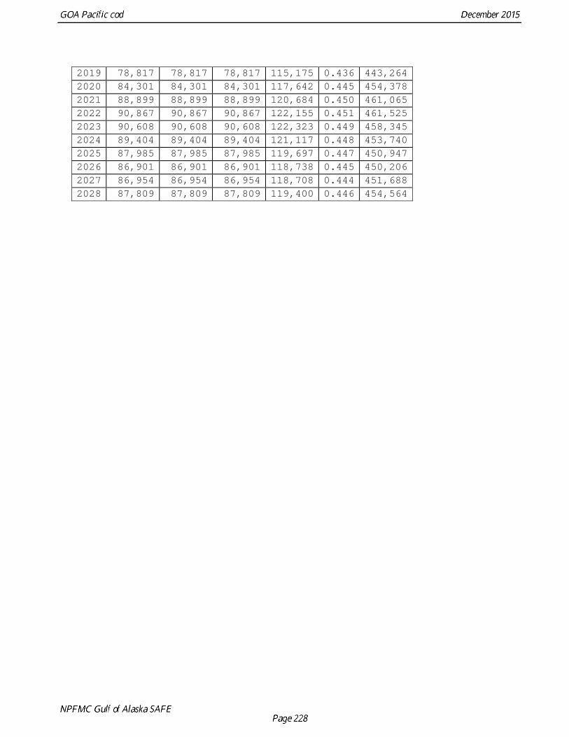
Scenario 7: In 2016 and 2017, F is set equal to max FABC, and in all subsequent years, F is set equal to FOFL. (Rationale: This scenario determines whether a stock is approaching an overfished condition. If the stock is expected to be above its MSY level in 2028 under this scenario, then the stock is not approaching an overfished condition.)
Projections and Status Determination Projections corresponding to the standard scenarios are shown for this year’s model in Table 2.21 (note that Scenarios 1 and 2 are identical in this case, because the recommended ABC is equal to the maximum permissible ABC).
In addition to the seven standard harvest scenarios, Amendments 48/48 to the BSAI and GOA Groundfish Fishery Management Plans require projections of the likely OFL two years into the future. While Scenario 6 gives the best estimate of OFL for 2016, it does not provide the best estimate of OFL for 2017, because the mean 2017 catch under Scenario 6 is predicated on the 2016 catch being equal to the 2016 OFL, whereas the actual 2016 catch will likely be less than the 2016 OFL.
Under the MSFCMA, the Secretary of Commerce is required to report on the status of each U.S. fishery with respect to overfishing. This report involves the answers to three questions: 1) Is the stock being subjected to overfishing? 2) Is the stock currently overfished? 3) Is the stock approaching an overfished condition?
Is the stock being subjected to overfishing? The official catch estimate for the most recent complete year (2014) is 84,840 t. This is less than the 2014 OFL of 140,300 t. Therefore, the stock is not being subjected to overfishing.
Harvest Scenarios #6 and #7 are intended to permit determination of the status of a stock with respect to its minimum stock size threshold (MSST). Any stock that is below its MSST is defined to be overfished. Any stock that is expected to fall below its MSST in the next two years is defined to be approaching an overfished condition. Harvest Scenarios #6 and #7 are used in these determinations as follows:
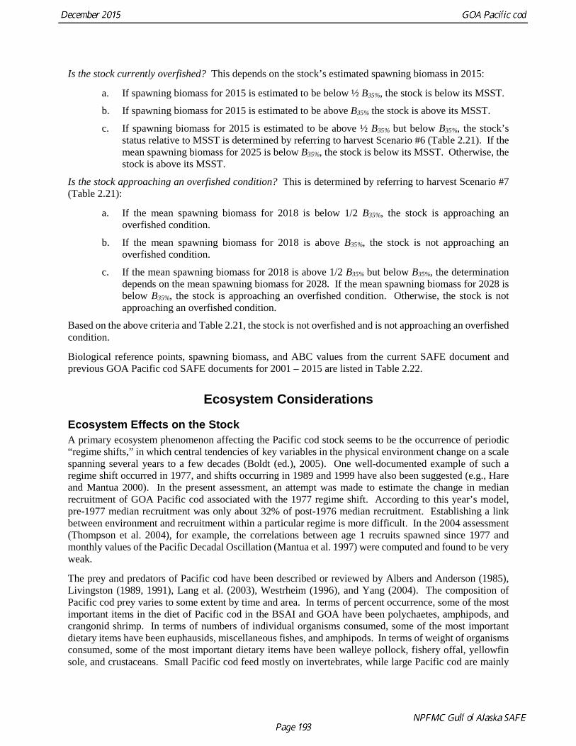
Is the stock currently overfished? This depends on the stock’s estimated spawning biomass in 2015:
a. If spawning biomass for 2015 is estimated to be below ½ B35%, the stock is below its MSST.
b. If spawning biomass for 2015 is estimated to be above B35% the stock is above its MSST.
c. If spawning biomass for 2015 is estimated to be above ½ B35% but below B35%, the stock’s status relative to MSST is determined by referring to harvest Scenario #6 (Table 2.21). If the mean spawning biomass for 2025 is below B35%, the stock is below its MSST. Otherwise, the stock is above its MSST.
Is the stock approaching an overfished condition? This is determined by referring to harvest Scenario #7 (Table 2.21):
a. If the mean spawning biomass for 2018 is below 1/2 B35%, the stock is approaching an overfished condition.
b. If the mean spawning biomass for 2018 is above B35%, the stock is not approaching an overfished condition.
c. If the mean spawning biomass for 2018 is above 1/2 B35% but below B35%, the determination depends on the mean spawning biomass for 2028. If the mean spawning biomass for 2028 is below B35%, the stock is approaching an overfished condition. Otherwise, the stock is not approaching an overfished condition.
Based on the above criteria and Table 2.21, the stock is not overfished and is not approaching an overfished condition.
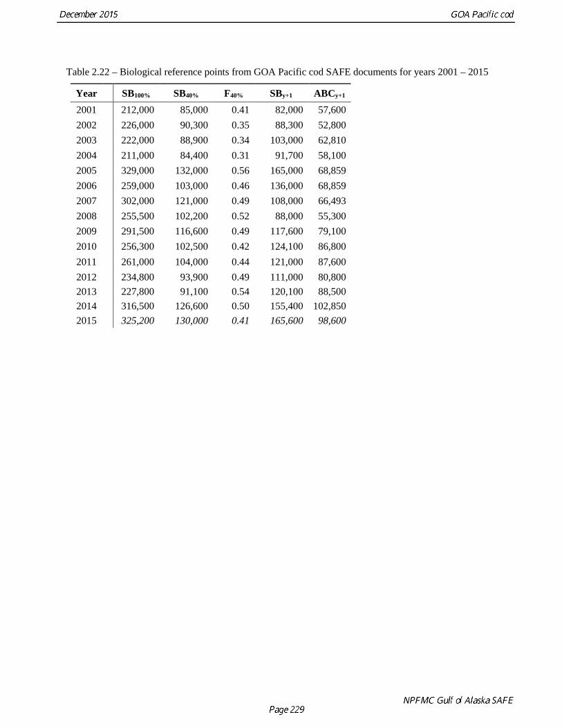
Biological reference points, spawning biomass, and ABC values from the current SAFE document and previous GOA Pacific cod SAFE documents for 2001 – 2015 are listed in Table 2.22.
Ecosystem Considerations
Ecosystem Effects on the Stock A primary ecosystem phenomenon affecting the Pacific cod stock seems to be the occurrence of periodic “regime shifts,” in which central tendencies of key variables in the physical environment change on a scale spanning several years to a few decades (Boldt (ed.), 2005). One well-documented example of such a regime shift occurred in 1977, and shifts occurring in 1989 and 1999 have also been suggested (e.g., Hare and Mantua 2000). In the present assessment, an attempt was made to estimate the change in median recruitment of GOA Pacific cod associated with the 1977 regime shift. According to this year’s model, pre-1977 median recruitment was only about 32% of post-1976 median recruitment. Establishing a link between environment and recruitment within a particular regime is more difficult. In the 2004 assessment (Thompson et al. 2004), for example, the correlations between age 1 recruits spawned since 1977 and monthly values of the Pacific Decadal Oscillation (Mantua et al. 1997) were computed and found to be very weak.
The prey and predators of Pacific cod have been described or reviewed by Albers and Anderson (1985), Livingston (1989, 1991), Lang et al. (2003), Westrheim (1996), and Yang (2004). The composition of Pacific cod prey varies to some extent by time and area. In terms of percent occurrence, some of the most important items in the diet of Pacific cod in the BSAI and GOA have been polychaetes, amphipods, and crangonid shrimp. In terms of numbers of individual organisms consumed, some of the most important dietary items have been euphausids, miscellaneous fishes, and amphipods. In terms of weight of organisms consumed, some of the most important dietary items have been walleye pollock, fishery offal, yellowfin sole, and crustaceans. Small Pacific cod feed mostly on invertebrates, while large Pacific cod are mainly
piscivorous. Predators of Pacific cod include Pacific cod, halibut, salmon shark, northern fur seals, Steller sea lions, harbor porpoises, various whale species, and tufted puffin. Major trends in the most important prey or predator species could be expected to affect the dynamics of Pacific cod to some extent.
Fishery Effects on the Ecosystem Potentially, fisheries for Pacific cod can have effects on other species in the ecosystem through a variety of mechanisms, for example by relieving predation pressure on shared prey species (i.e., species which serve as prey for both Pacific cod and other species), by reducing prey availability for predators of Pacific cod, by altering habitat, by imposing bycatch mortality, or by “ghost fishing” caused by lost fishing gear.
Incidental Catch of Nontarget Species Incidental catches of nontarget species in each year 2005-2014 are shown Table 2.6. In terms of average catch over the time series, only sea stars account for more than 250 t per year.
Steller Sea Lions Sinclair and Zeppelin (2002) showed that Pacific cod was one of the four most important prey items of Steller sea lions in terms of frequency of occurrence averaged over years, seasons, and sites, and was especially important in winter. Pitcher (1981) and Calkins (1998) also showed Pacific cod to be an important winter prey item in the GOA and BSAI, respectively. Furthermore, the size ranges of Pacific cod harvested by the fisheries and consumed by Steller sea lions overlap, and the fishery operates to some extent in the same geographic areas used by Steller sea lion as foraging grounds (Livingston (ed.), 2002).
The Fisheries Interaction Team of the Alaska Fisheries Science Center has been engaged in research to determine the effectiveness of recent management measures designed to mitigate the impacts of the Pacific cod fisheries (among others) on Steller sea lions. Results from studies conducted in 2002-2003 were summarized by Conners et al. (2004). These studies included a tagging feasibility study, which may evolve into an ongoing research effort capable of providing information on the extent and rate to which Pacific cod move in and out of various portions of Steller sea lion critical habitat. Nearly 6,000 cod with spaghetti tags were released, of which approximately 1,000 had been returned as of September 2003.
Seabirds The following is a summary of information provided by Livingston (ed., 2002): In both the BSAI and GOA, the northern fulmar (Fulmarus glacialis) comprises the majority of seabird bycatch, which occurs primarily in the longline fisheries, including the hook and line fishery for Pacific cod (Tables 2.30b and 2.30b). Shearwater (Puffinus spp.) distribution overlaps with the Pacific cod longline fishery in the Bering Sea, and with trawl fisheries in general in both the Bering Sea and GOA. Black-footed albatross (Phoebastria nigripes) is taken in much greater numbers in the GOA longline fisheries than the Bering Sea longline fisheries, but is not taken in the trawl fisheries. The distribution of Laysan albatross (Phoebastria immutabilis) appears to overlap with the longline fisheries in the central and western Aleutians. The distribution of short-tailed albatross (Phoebastria albatrus) also overlaps with the Pacific cod longline fishery along the Aleutian chain, although the majority of the bycatch has taken place along the northern portion of the Bering Sea shelf edge (in contrast, only two takes have been recorded in the GOA). Some success has been obtained in devising measures to mitigate fishery-seabird interactions. For example, on vessels larger than 60 ft. LOA, paired streamer lines of specified performance and material standards have been found to reduce seabird incidental take significantly.
Fishery Usage of Habitat The following is a summary of information provided by Livingston (ed., 2002): The longline and trawl fisheries for Pacific cod each comprise an important component of the combined fisheries associated with the respective gear type in each of the three major management regions (BS, AI, and GOA). Looking at each gear type in each region as a whole (i.e., aggregating across all target species) during the period 1998-2001, the total number of observed sets was as follows:
In the BS, both longline and trawl effort was concentrated north of False Pass (Unimak Island) and along the shelf edge represented by the boundary of areas 513, 517 (in addition, longline effort was concentrated along the shelf edge represented by the boundary of areas 521-533). In the AI, both longline and trawl effort were dispersed over a wide area along the shelf edge. The catcher vessel longline fishery in the AI occurred primarily over mud bottoms. Longline catcher-processors in the AI tended to fish more over rocky bottoms. In the GOA, fishing effort was also dispersed over a wide area along the shelf, though pockets of trawl effort were located near Chirikof, Cape Barnabus, Cape Chiniak and Marmot Flats. The GOA longline fishery for Pacific cod generally took place over gravel, cobble, mud, sand, and rocky bottoms, in depths of 25 fathoms to 140 fathoms.
Impacts of the Pacific cod fisheries on essential fish habitat were further analyzed in an environmental impact statement by NMFS (2005).
Data Gaps and Research Priorities Understanding of the above ecosystem considerations would be improved if future research were directed toward closing certain data gaps. Such research would have several foci, including the following: 1) ecology of the Pacific cod stock, including spatial dynamics, trophic and other interspecific relationships, and the relationship between climate and recruitment; 2) behavior of the Pacific cod fishery, including spatial dynamics; 3) determinants of trawl survey catchability and selectivity; 4) age determination; 5) ecology of species taken as bycatch in the Pacific cod fisheries, including estimation of biomass, carrying capacity, and resilience; and 6) ecology of species that interact with Pacific cod, including estimation of biomass, carrying capacity, and resilience.
Acknowledgements Jon Short and Delsa Anderl provided age data; Delsa Anderl provided more details on the 1987 survey age data. Peter Munro provided information on the 27-cm split of the GOA NMFS bottom trawl survey data. Sonya Elmejjati (ADF&G) and Elisa Russ (ADF&G) provided size composition data from the State of Alaska-managed Pacific cod fishery. Rick Methot developed the Stock Synthesis software used to conduct this assessment, and Ian Taylor developed the R package r4ss and answered numerous questions about the software. Jim Ianelli and Peter Hulson provided the code for the random effects model area apportion calculations. Grant Thompson and the GOA Groundfish Plan Team provided reviews of this assessment. Many NMFS survey personnel and countless fishery observers collected most of the raw data that were used in this assessment.
Literature Cited Albers, W. D., and P. J. Anderson. 1985. Diet of Pacific cod, Gadus macrocephalus, and predation on the
northern pink shrimp, Pandalus borealis, in Pavlof Bay, Alaska. Fish. Bull., U.S. 83:601-610. A’mar, T., Thompson, G., Martin, M., and W. Palsson. 2012. Assessment of the Pacific cod stock in the
Gulf of Alaska. In Plan Team for Groundfish Fisheries of the Gulf of Alaska (compiler), Stock assessment and fishery evaluation report for the groundfish resources of the Gulf of Alaska, p. 183-322. North Pacific Fishery Management Council, 605 W. 4th Avenue Suite 306, Anchorage, AK 99501
Bakkala, R. G., and V. G. Wespestad. 1985. Pacific cod. In R. G. Bakkala and L. L. Low (editors), Condition of groundfish resources of the eastern Bering Sea and Aleutian Islands region in 1984, p. 37-49. U.S. Dep. Commer., NOAA Tech. Memo. NMFS F/NWC-83.
Boldt, J. (editor). 2005. Ecosystem Considerations for 2006. North Pacific Fishery Management Council, 605 West 4th Ave., Suite 306, Anchorage, AK 99501.
Calkins, D. G. 1998. Prey of Steller sea lions in the Bering Sea. Biosphere Conservation 1:33-44. Fournier, D. 1983. An analysis of the Hecate Strait Pacific cod fishery using an age-structured model
incorporating density-dependent effects. Can. J. Fish. Aquat. Sci. 40:1233-1243. Fournier, D., and C. P. Archibald. 1982. A general theory for analyzing catch at age data. Can. J. Fish.
Aquat. Sci. 38:1195-1207. Fournier, D.A., H. J. Skaug, J. Ancheta, J. Ianelli, A. Magnusson, M. N. Maunder, A. Nielsen, and J. Sibert.
2012. AD Model Builder: using automatic differentiation for statistical inference of highly parameterized complex nonlinear models. Optim. Methods Softw. 27:233-249.
Greer-Walker, M. 1970. Growth and development of the skeletal muscle fibres of the cod (Gadus morhua L.). Journal du Conseil 33:228-244.
Gregory, R. S., C. Morris, and B. Newton. In review. Relative strength of the 2007 and 2008 year-classes, from nearshore surveys of demersal age 0 Atlantic cod in Newman Sound, Bonavista Bay. Can. Sci. Advis. Sec. Res. Doc. series./xxx.
Hare, S. R., and N. J. Mantua. 2000. Empirical evidence for North Pacific regime shifts in 1977 and 1989. Progress in Oceanography 47:103-146.
Hiatt, T., R. Felthoven, M. Dalton, B. Garber-Yonts, A. Haynie, K. Herrmann, D. Lew, J. Sepez, C. Seung, L. Sievanen, and the staff of Northern Economics. 2007. Stock Assessment and Fishery Evaluation Report for the Groundfish Fisheries of the Gulf of Alaska and Bering Sea/Aleutian Islands Area: Economic Status of the Groundfish Fisheries off Alaska, 2006. Economic and Social Sciences Research Program, Resource Ecology and Fisheries Management Division, Alaska Fisheries Science Center, NMFS, NOAA, 7600 Sand Point Way N.E., Seattle, Washington 98115-6349. 353 p.
Jung, S., I. Choi, H. Jin, D.-w. Lee, H.-k. Cha, Y. Kim, and J.-y. Lee. 2009. Size-dependent mortality formulation for isochronal fish species based on their fecundity: an example of Pacific cod (Gadus macrocephalus) in the eastern coastal areas of Korea. Fisheries Research 97:77-85.
Ketchen, K.S. 1964. Preliminary results of studies on a growth and mortality of Pacific cod (Gadus macrocephalus) in Hecate Strait, British Columbia. J. Fish. Res. Bd. Canada 21:1051-1067.
Lang, G. M., C. W. Derrah, and P. A. Livingston. 2003. Groundfish food habits and predation on commercially important prey species in the Eastern Bering Sea from 1993 through 1996. Alaska Fisheries Science Center Processed Report 2003-04. Alaska Fisheries Science Center, 7600 Sand Point Way NE., Seattle, WA 98115-6349. 351 p.
Livingston, P. A. 1989. Interannual trends in Pacific cod, Gadus macrocephalus, predation on three commercially important crab species in the eastern Bering Sea. Fish. Bull., U.S. 87:807-827.
Livingston, P. A. 1991. Pacific cod. In P. A. Livingston (editor), Groundfish food habits and predation on commercially important prey species in the eastern Bering Sea from 1984 to 1986, p. 31-88. U.S. Dept. Commer, NOAA Tech. Memo. NMFS F/NWC-207.
Livingston, P. A. (editor). 2003. Ecosystem Considerations for 2003. North Pacific Fishery Management Council, 605 West 4th Ave., Suite 306, Anchorage, AK 99501.
Low, L. L. 1974. A study of four major groundfish fisheries of the Bering Sea. Ph.D. Thesis, Univ. Washington, Seattle, WA. 240 p.
Mantua, N. J., Hare, S. R., Zhang, Y., Wallace, J. M., & Francis, R. C. 1997. A Pacific interdecadal climate oscillation with impacts on salmon production. Bulletin of the American Meteorological Society 78, 1069-1079.
Methot, R. D. 1986. Synthetic estimates of historical abundance and mortality for northern anchovy, Engraulis mordax. NMFS, Southwest Fish. Cent., Admin. Rep. LJ 86-29, La Jolla, CA.
Methot, R. D. 1990. Synthesis model: An adaptable framework for analysis of diverse stock assessment data. Int. N. Pac. Fish. Comm. Bull. 50:259-277.
Methot, R. D. 1998. Application of stock synthesis to NRC test data sets. In V. R. Restrepo (editor), Analyses of simulated data sets in support of the NRC study on stock assessment methods, p. 59-80. U.S. Dep. Commer., NOAA Tech. Memo. NMFS-F/SPO-30.
Methot, R. D. 2000. Technical description of the stock synthesis assessment program. U.S. Dep. Commer., NOAA Tech. Memo. NMFS-NWFSC-43, 46 p.
Methot, R. D. 2005a. Technical description of the Stock Synthesis II Assessment Program. Unpubl. manuscr. National Marine Fisheries Service, Northwest Fisheries Science Center, 2725 Montlake Blvd. East, Seattle, WA 98112-2097. 54 p.
Methot, R. D. 2005b. User manual for the assessment program Strock Synthesis 2 (SS2), Model Version 1.19. National Marine Fisheries Service, Northwest Fisheries Science Center, 2725 Montlake Blvd. East, Seattle, WA 98112-2097. 47 p.
Methot, R. D. 2007. User manual for the integrated analysis program Stock Synthesis 2 (SS2), Model Version 2.00c. National Marine Fisheries Service, Northwest Fisheries Science Center, 2725 Montlake Blvd. East, Seattle, WA 98112-2097. 47 p.
Methot, R. D. 2013. User Manual for Stock Synthesis, Model Version 3.24q. Unpublished manuscript. 150 p.
Methot, R. D., and Wetzell, C. R. 2013. Stock synthesis: A biological and statistical framework for fish stock assessment and fishery management. Fish. Rsch. 142:86-99.
National Marine Fisheries Service (NMFS). 2005. Final environmental impact statement for essential fish habitat identification and conservation in Alaska. National Marine Fisheries Service, Alaska Region. P.O. Box 21668, Juneau, AK 99802-1668.
Nichol, D. G., T. Honkalehto, and G. G. Thompson. 2007. Proximity of Pacific cod to the sea floor: Using archival tags to estimate fish availability to research bottom trawls. Fisheries Research 86:129-135.
Ona, E., and O. R. Godø. 1990. Fish reaction to trawling noise: the significance for trawl sampling. Rapports et Procès-Verbaux des Réunions du Conseil International pour l’Exploration de la Mer 189: 159–166.
Pitcher, K. W. 1981. Prey of Steller sea lion, Eumetopias jubatus, in the Gulf of Alaska. Fishery Bulletin 79:467-472.
Savin, A. B. 2008. Seasonal distribution and Migrations of Pacific cod Gadus macrocephalus (Gadidae) in Anadyr Bay and adjacent waters. Journal of Ichythyology 48:610-621.
Shimada, A. M., and D. K. Kimura. 1994. Seasonal movements of Pacific cod (Gadus macrocephalus) in the eastern Bering Sea and adjacent waters based on tag-recapture data. U.S. Natl. Mar. Fish. Serv., Fish. Bull. 92:800-816.
Sinclair, E.S. and T. K. Zeppelin. 2002. Seasonal and spatial differences in diet in the western stock of Steller sea lions (Eumetopias jubatus). Journal of Mammalogy 83(4).
Spies I. 2012. Landscape genetics reveals population subdivision in Bering Sea and Aleutian Islands Pacific cod. Transactions of the American Fisheries Society 141:1557-1573.
Stark, J. W. 2007. Geographic and seasonal variations in maturation and growth of female Pacific cod (Gadus macrocephalus) in the Gulf of Alaska and Bering Sea. Fish. Bull. 105:396–407.
Thompson, G., T. A’mar, and W. Palsson. 2011. Assessment of the Pacific cod stock in the Gulf of Alaska. In Plan Team for Groundfish Fisheries of the Gulf of Alaska (compiler), Stock assessment and fishery evaluation report for the groundfish resources of the Gulf of Alaska, p. 161-306. North Pacific Fishery Management Council, 605 W. 4th Avenue Suite 306, Anchorage, AK 99501
Thompson, G. G., and M. E. Conners. 2007. Report of the Pacific cod technical workshop held at the Alaska Fisheries Science Center, April 24-25, 2007. Unpubl. manuscr., Alaska Fisheries Science Center, Resource Ecology and Fisheries Management Division, 7600 Sand Point Way NE., Seattle, WA 98115-6349. 56 p.
Thompson, G. G., and M. W. Dorn. 2005. Assessment of the Pacific cod stock in the Gulf of Alaska. In Plan Team for Groundfish Fisheries of the Gulf of Alaska (compiler), Stock assessment and fishery evaluation report for the groundfish resources of the Gulf of Alaska, p. 155-244. North Pacific Fishery Management Council, 605 W. 4th Avenue Suite 306, Anchorage, AK 99501.
Thompson, G., M. Dorn, and D. Nichol. 2006. Assessment of the Pacific cod stock in the Gulf of Alaska. In Plan Team for Groundfish Fisheries of the Gulf of Alaska (compiler), Stock assessment and fishery evaluation report for the groundfish resources of the Gulf of Alaska, p. 147-220. North Pacific Fishery Management Council, 605 W. 4th Avenue Suite 306, Anchorage, AK 99501.
Thompson, G., J. Ianelli, M. Dorn, D. Nichol, S. Gaichas, and K. Aydin. 2007a. Assessment of the Pacific cod stock in the Eastern Bering Sea and Aleutian Islands Area. In Plan Team for Groundfish Fisheries of the Bering Sea/Aleutian Islands (compiler), Stock assessment and fishery evaluation report for the groundfish resources of the Bering Sea/Aleutian Islands regions, p. 209-327. North Pacific Fishery Management Council, 605 W. 4th Avenue Suite 306, Anchorage, AK 99501.
Thompson, G., J. Ianelli, M. Dorn, and M. Wilkins. 2007b. Assessment of the Pacific cod stock in the Gulf of Alaska. In Plan Team for Groundfish Fisheries of the Gulf of Alaska (compiler), Stock assessment and fishery evaluation report for the groundfish resources of the Gulf of Alaska, p. 169-194. North Pacific Fishery Management Council, 605 W. 4th Avenue Suite 306, Anchorage, AK 99501.
Thompson, G., J. Ianelli, M. Dorn, and M. Wilkins. 2009. Assessment of the Pacific cod stock in the Gulf of Alaska. In Plan Team for Groundfish Fisheries of the Gulf of Alaska (compiler), Stock assessment and fishery evaluation report for the groundfish resources of the Gulf of Alaska, p. 165-352. North Pacific Fishery Management Council, 605 W. 4th Avenue Suite 306, Anchorage, AK 99501.
Thompson, G., J. Ianelli, M. Dorn, and M. Wilkins. 2010. Assessment of the Pacific cod stock in the Gulf of Alaska. In Plan Team for Groundfish Fisheries of the Gulf of Alaska (compiler), Stock assessment and fishery evaluation report for the groundfish resources of the Gulf of Alaska, p. 157-328. North Pacific Fishery Management Council, 605 W. 4th Avenue Suite 306, Anchorage, AK 99501.
Thompson, G. G., and R. D. Methot. 1993. Pacific cod. In Plan Team for Groundfish Fisheries of the Bering Sea/Aleutian Islands (editor), Stock assessment and fishery evaluation report for the groundfish resources of the Bering Sea/Aleutian Islands region as projected for 1994, chapter 2. North Pacific Fishery Management Council, 605 W. 4th Avenue Suite 306, Anchorage, AK 99501.
Thompson, G. G., and A. M. Shimada. 1990. Pacific cod. In L. L. Low and R. E. Narita (editors), Condition of groundfish resources of the eastern Bering Sea-Aleutian Islands region as assessed in 1988, p. 44-66. U.S. Dep. Commer., NOAA Tech. Memo. NMFS F/NWC-178.
Thompson, G. G, and H. H. Zenger. 1993. Pacific cod. In Plan Team for Groundfish Fisheries of the Gulf of Alaska (editor), Stock assessment and fishery evaluation report for the groundfish resources of
the Gulf of Alaska as projected for 1994, chapter 2. North Pacific Fishery Management Council, 605 W. 4th Avenue Suite 306, Anchorage, AK 99501.
Thompson, G. G, and H. H. Zenger. 1994. Pacific cod. In Plan Team for Groundfish Fisheries of the Gulf of Alaska (editor), Stock assessment and fishery evaluation report for the groundfish resources of the Gulf of Alaska as projected for 1995, chapter 2. North Pacific Fishery Management Council, 605 W. 4th Avenue Suite 306, Anchorage, AK 99501.
Thompson, G. G., and H. H. Zenger. 1995. Pacific cod. In Plan Team for the Groundfish Fisheries of the Gulf of Alaska (editor), Stock assessment and fishery evaluation report for the groundfish resources of the Gulf of Alaska as projected for 1996, chapter 2. North Pacific Fishery Management Council, 605 W. 4th Avenue Suite 306, Anchorage, AK 99501.
Thompson, G. G., H. H. Zenger, and M. K. Dorn. 2002. Assessment of the Pacific cod stock in the Gulf of Alaska. In Plan Team for the Groundfish Fisheries of the Gulf of Alaska (compiler), Stock Assessment and Fishery Evaluation Report for the Groundfish Resources of the Gulf of Alaska p. 89-167. North Pacific Fishery Management Council, 605 West 4th Ave., Suite 306, Anchorage, AK 99501.
Thompson, G. G., H. H. Zenger, and M. K. Dorn. 2004. Assessment of the Pacific cod stock in the Gulf of Alaska. In Plan Team for the Groundfish Fisheries of the Gulf of Alaska (compiler), Stock Assessment and Fishery Evaluation Report for the Groundfish Resources of the Gulf of Alaska p. 131-232. North Pacific Fishery Management Council, 605 West 4th Ave., Suite 306, Anchorage, AK 99501.
Ueda, Y., Y. Narimatsu, T. Hattori, M. Ito, D. Kitagawa, N. Tomikawa, and T. Matsuishi. 2006. Fishing efficiency estimated based on the abundance from virtual population analysis and bottom-trawl surveys of Pacific cod (Gadus macrocephalus) in the waters off the Pacific coast of northern Honshu, Japan. Nippon Suisan Gakkaishi 72:201-209.
Wespestad, V., R. Bakkala, and J. June. 1982. Current abundance of Pacific cod (Gadus macrocephalus) in the eastern Bering Sea and expected abundance in 1982-1986. NOAA Tech. Memo. NMFS F/NWC-25, 26 p.
Westrheim, S. J. 1996. On the Pacific cod (Gadus macrocephalus) in British Columbia waters, and a comparison with Pacific cod elsewhere, and Atlantic cod (G. morhua). Can. Tech. Rep. Fish. Aquat. Sci. 2092. 390 p.
Yang, M-S. 2004. Diet changes of Pacific cod (Gadus macrocephalus) in Pavlof Bay associated with climate changes in the Gulf of Alaska between 1980 and 1995. U.S. Natl. Mar. Fish. Serv., Fish. Bull. 102:400-405.
Tables Table 2.1. Catch (t) for 1991 through 2015 by jurisdiction and gear type (as of 2015-10-19)
Table 2.2 History of Pacific cod catch (t, includes catch from State waters), Federal TAC (does not include State guideline harvest level), ABC, and OFL. ABC was not used in management of GOA groundfish prior to 1986. Catch for 2015 is current through 2015-10-19. The values in the column labeled “TAC” correspond to “optimum yield” for the years 1980-1986, “target quota” for the year 1987, and true TAC for the years 1988-present. The ABC value listed for 1987 is the upper bound of the range. Source: NPFMC staff.
Table 2.7 Catch (t) of Pacific cod by year, gear, and season for the years 1991-2015 as configured in the stock assessment models; the values for 2015 seasons 4 and 5 (Sep – Oct and Nov – Dec) were estimated given the average fraction of catch in each month for 2010 – 2014 and the average fraction of each gear type in seasons 4 and 5 for 2010 – 2014 (as of 2015-10-02).
Trawl Longline Pot Year Jan-Apr May-Aug Sep-Dec Total Jan-Apr May-Aug Sep-Dec Total Jan-Apr May-Aug Sep-Dec Total 1991 55,862 778 1,493 58,133 7,052 540 72 7,664 9,413 183 934 10,530
Table 2.8 – Noncommercial fishery catch (in t); total source amounts less than 1 mt were omitted (AFSC for GOA bottom trawl survey values; AKFIN for other values, as of 2015-10-19)
Table 2.12 Pacific cod abundance measured in biomass (t) and numbers of fish (1000s), as assessed by the GOA bottom trawl survey. Point estimates are shown along with coefficients of variation. The two right-hand sections show the total abundance divided into fish 27 cm or larger and fish smaller than 27 cm (totals are very slightly different in the first four years due to exclusion of tows with no length data from the strata extrapolations).
Table 2.15 – Schedules of estimated population length (cm) and weight (kg) by season and age from Model 3 – ¼ fsh. Season 1=Jan-Feb, Season 2=Mar-Apr, Season 3=May-Aug, Season 4=Sep-Oct, Season 5=Nov-Dec. Lengths and weights correspond to season mid-points.
Table 2.21 – Results for the projection scenarios from Model 3 – ¼ fsh. ABC, OFL, Catch, Female Spawning Stock Biomass (SSB), and Total Biomass (Total Bio) in metric tons. Fishing mortality (F) is also presented.
Figures Fig. 2.1 – Fishery catches by season and gear (AKFIN; as of 2015-10-02)
Year
Land
ings
(mt)
aggr
egat
ed a
cros
s se
ason
s
020
000
4000
060
000
8000
0
1980 1985 1990 1995 2000 2005 2010 2015
Jan-Apr_Trawl_Fishery
May-Aug_Trawl_Fishery
Sep-Dec_Trawl_Fishery
Jan-Apr_Longline_Fishery
May-Aug_Longline_Fishery
Sep-Dec_Longline_Fishery
Jan-Apr_Pot_Fishery
May-Aug_Pot_Fishery
Sep-Dec_Pot_Fishery
Fig. 2.2 – GOA NMFS bottom trawl survey biomass estimates for Pacific cod, with 95% confidence interval
1985 1990 1995 2000 2005 2010 2015
0e+0
02e
+05
4e+0
56e
+05
8e+0
51e
+06
Est
imat
ed b
iom
ass
(mt)
Fig. 2.3 – GOA NMFS survey abundance estimates for Pacific cod, with 95% confidence interval
1985 1990 1995 2000 2005 2010 2015
0e+0
02e
+08
4e+0
86e
+08
8e+0
8
Est
imat
ed n
umbe
r
Total abundance27-plus abundanceSub-27 abundance
Fig. 2.4 – GOA NMFS bottom trawl survey biomass estimates by area (in t)
0
50
100
150
200
250
300
350
400
450
500
1996 1999 2001 2003 2005 2007 2009 2011 2013 2015
Met
ric to
nnes
Thou
sand
sNMFS survey biomass estimates of Pacific cod, by
area
610
620
630
640
650
Fig. 2.5 – GOA NMFS bottom trawl survey abundance estimates by area (in numbers)
0
50
100
150
200
250
300
1996 1999 2001 2003 2005 2007 2009 2011 2013 2015
Milli
ons
NMFS survey abundance estimates of Pacific cod, by area
610
620
630
640
650
Fig. 2.6 – GOA NMFS bottom trawl survey population length composition estimates for Pacific cod, by cm
0 20 40 60 80 100
0.00
0.02
0.04
1984
0 20 40 60 80 100
0.00
0.02
1987
0 20 40 60 80 100
0.00
0.02
0.04
1990
0 20 40 60 80 100
0.00
0.02
0.04
1993
0 20 40 60 80 100
0.00
0.02
1996
0 20 40 60 80 100
0.00
00.
015
0.03
0
1999
0 20 40 60 80 100
0.00
00.
010
0.02
0
2001
0 20 40 60 80 100
0.00
0.02
0.04
2003
0 20 40 60 80 100
0.00
0.02
0.04
2005
0 20 40 60 80 100
0.00
0.02
0.04
2007
0 20 40 60 80 100
0.00
0.04
2009
0 20 40 60 80 100
0.00
0.02
0.04
2011
0 20 40 60 80 100
0.00
0.02
2013
0 20 40 60 80 100
0.00
0.02
0.04
2015
Fig. 2.7 – GOA NMFS bottom trawl survey population age composition estimates for Pacific cod
0 2 4 6 8 10 12
0.00
0.10
0.20
0.30
1987
0 2 4 6 8 10 12
0.00
0.10
0.20
1990
0 2 4 6 8 10 12
0.00
0.10
0.20
1993
0 2 4 6 8 10 12
0.00
0.10
0.20 1996
0 2 4 6 8 10 120.
000.
100.
20
1999
0 2 4 6 8 10 12
0.00
0.05
0.10
0.15
0.20
2001
0 2 4 6 8 10 12
0.00
0.10
0.20
2003
0 2 4 6 8 10 12
0.00
0.10
0.20
2005
0 2 4 6 8 10 12
0.00
0.10
0.20
0.30
2007
0 2 4 6 8 10 12
0.00
0.10
0.20
2009
0 2 4 6 8 10 12
0.0
0.1
0.2
0.3
0.4
2011
0 2 4 6 8 10 12
0.00
0.05
0.10
0.15
0.20
2013
Fig. 2.8 – Estimates of spawning biomass for Models 0, 1, 2, and 3
Year
Spa
wni
ng o
utpu
t
1980 1990 2000 2010 2015
0
200
400
600
Model 2
Model 3
Model 1
Model 0
Fig. 2.9 – Estimates of age-0 recruits (billions) for Models 0, 1, 2, and 3
Year
Age
-0 re
crui
ts (b
illio
ns)
Model 2
Model 3
Model 1
Model 0
1980 1990 2000 2010 2015
0.0
0.5
1.0
1.5
Fig. 2.10 – Fits (solid lines) to the 27-plus survey abundance estimates (solid circles, with 95% confidence intervals) for Models 2 and 3, and the full survey abundance estimates (solid circles, with 95% confidence intervals) for Models 0 and 1
Figure 2.11 – Estimates of spawning biomass for Models 2 and 3 with different weights on fitting to the fishery catch-at-length data
Year
Spa
wni
ng o
utpu
t
1980 1990 2000 2010 2015
0
100
200
300
400
500
600
700
Model 2
Model 2 - 3/4 fsh
Model 2 - 1/2 fsh
Model 2 - 1/4 fsh
Model 3
Model 3 - 3/4 fsh
Model 3 - 1/2 fsh
Model 3 - 1/4 fsh
Figure 2.12 – Estimates of age-0 recruits for Models 2 and 3 with different weights on fitting to the fishery catch-at-length data
Year
Age
-0 re
crui
ts (b
illio
ns)
Model 2
Model 2 - 3/4 fsh
Model 2 - 1/2 fsh
Model 2 - 1/4 fsh
Model 3
Model 3 - 3/4 fsh
Model 3 - 1/2 fsh
Model 3 - 1/4 fsh
1980 1990 2000 2010 2015
0.0
0.2
0.4
0.6
0.8
1.0
1.2
Figure 2.13 – Fits (solid lines) to the 27-plus survey abundance estimates (solid circles, with 95% confidence intervals) for Models 2 and 3 with different weights on fitting to the fishery catch-at-length data
Fig. 2.14 – Estimates of total (age 0+) biomass for Model 3 – ¼ fsh
1980 1990 2000 2010
020
0000
4000
0060
0000
8000
0010
0000
012
0000
0Total biomass (mt) at beginning of season 2
Year
Tota
l bio
mas
s (m
t) at
beg
inni
ng o
f sea
son
2
Fig. 2.15 – Estimates of female spawning biomass for Model 3 – ¼ fsh
1980 1990 2000 2010
0e+0
01e
+05
2e+0
53e
+05
4e+0
55e
+05
6e+0
5Spawning output with ~95% asymptotic intervals
Year
Spa
wni
ng o
utpu
t
-
-
Fig. 2.16 – Estimates of age-0 recruits for Model 3 – ¼ fsh
1980 1990 2000 2010
020
0000
4000
0060
0000
8000
0010
0000
012
0000
014
0000
0Age-0 recruits (1,000s) with ~95% asymptotic interval
Year
Age
-0 re
crui
ts (1
,000
s)
Fig. 2.17 – Fit to the survey abundance estimates with 95% confidence intervals for Model 3 – ¼ fsh
1985 1990 1995 2000 2005 2010 2015
11.5
12.0
12.5
13.0
Log index Trawl_Survey
Year
Log
inde
x
Season1
Season2
Season3
Season4
Season5
1985 1990 1995 2000 2005 2010 2015
0e+0
01e
+05
2e+0
53e
+05
4e+0
55e
+05
Index Trawl_Survey
Year
Inde
x
Fig. 2.18 – Estimates of spawning biomass (t) and age-0 recruits for Model 3 – ¼ fsh; the solid black line is the median, and the solid green line is the bias-adjusted median
0e+00 1e+05 2e+05 3e+05 4e+05 5e+05
0e+0
02e
+05
4e+0
56e
+05
8e+0
51e
+06
Spawning biomass (mt)
Rec
ruitm
ent (
1,00
0s)
1977
2002
2015
Exp. recruitment
Exp. recruitment after bias adj.
Estimated recruitments
Unfished equilibrium
Figure 2.19 – Estimates of the survey population length composition data (not used in model fitting) for Model 3 – ¼ fsh
Figure 2.20 – Fits to the survey population age composition data for Model 3 – ¼ fsh
Fig. 2.21 – Fits to the survey population length composition data for Model 3 – ¼ fsh
Fig. 2.22 – Fits to the survey conditional age-at-length data for Model 3 – ¼ fsh
40 60 80 1000
2
4
6
8
10
12
Age
1990.5
Conditional AAL plot, whole catch, Trawl_Survey
Length (cm)
40 60 80 1000.0
0.2
0.4
0.6
0.8
1.0
1.2
Length (cm)
Std
ev (
Age
) (y
r)
Observ ed (with 90% interv al)
Expected
40 60 80 1000
2
4
6
8
10
12
Age
1993.5
40 60 80 1000.0
0.2
0.4
0.6
0.8
1.0
1.2
Length (cm)
Std
ev (
Age
) (y
r)
40 60 80 1000
2
4
6
8
10
12
Age
1996.5
40 60 80 1000.0
0.5
1.0
1.5
Length (cm)
Std
ev (
Age
) (y
r)
40 60 80 1000
2
4
6
8
10
12
Age
1999.5
Conditional AAL plot, whole catch, Trawl_Survey
Length (cm)
40 60 80 1000.0
0.5
1.0
1.5
2.0
Length (cm)
Std
ev (
Age
) (y
r)
Observ ed (with 90% interv al)
Expected
40 60 80 1000
2
4
6
8
10
12
Age
2001.5
40 60 80 1000.0
0.5
1.0
1.5
Length (cm)
Std
ev (
Age
) (y
r)
40 60 80 1000
2
4
6
8
10
12
Age
2003.5
40 60 80 1000.0
0.5
1.0
1.5
Length (cm)
Std
ev (
Age
) (y
r)
40 60 80 1000
2
4
6
8
10
12
Age
2005.5
Conditional AAL plot, whole catch, Trawl_Survey
Length (cm)
40 60 80 1000.0
0.2
0.4
0.6
0.8
1.0
1.2
1.4
Length (cm)
Std
ev (
Age
) (y
r)
Observ ed (with 90% interv al)
Expected
40 60 80 1000
2
4
6
8
10
12
Age
2007.5
40 60 80 1000.0
0.5
1.0
1.5
Length (cm)
Std
ev (
Age
) (y
r)
40 60 80 1000
2
4
6
8
10
12
Age
2009.5
40 60 80 1000.0
0.5
1.0
1.5
Length (cm)
Std
ev (
Age
) (y
r)
40 60 80 1000
2
4
6
8
10
12
Age
2011.5
Conditional AAL plot, whole catch, Trawl_Survey
Length (cm)
40 60 80 1000.0
0.2
0.4
0.6
0.8
1.0
1.2
1.4
Length (cm)
Std
ev (
Age
) (y
r)
Observ ed (with 90% interv al)
Expected
40 60 80 1000
2
4
6
8
10
12
Age
2013.5
40 60 80 1000.0
0.2
0.4
0.6
0.8
1.0
1.2
1.4
Length (cm)
Std
ev (
Age
) (y
r)
Fig. 2.23 – Estimated length-at-age (cm) for Model 3 – ¼ fsh
Fig. 2.24 – Survey selectivity-at-age for Model 3 – ¼ fsh
Age (yr)0
510
1520
Yea
r
1980
1990
2000
2010
Selectivity
0.0
0.2
0.4
0.6
0.8
1.0
Time-varying selectivity for Trawl_Survey
Fig. 2.25 – Fishery selectivity-at-length by gear and season for Model 3 – ¼ fsh
Length (cm)20
4060
80100
Yea
r
1980
1990
2000
2010
Selectivity 0.2
0.4
0.6
0.8
1.0
Time-varying selectivity for Jan-Apr_Trawl_Fishery
Length (cm)20
4060
80100
Yea
r
1980
1990
2000
2010
Selectivity 0.2
0.4
0.6
0.8
1.0
Time-varying selectivity for May-Aug_Trawl_Fishery
Length (cm)20
4060
80100
Yea
r
1980
1990
2000
2010
Selectivity 0.2
0.4
0.6
0.8
1.0
Time-varying selectivity for Sep-Dec_Trawl_Fishery
Length (cm)20
4060
80100
Yea
r
1980
1990
2000
2010
Selectivity 0.2
0.4
0.6
0.8
1.0
Time-varying selectivity for Jan-Apr_Longline_Fishe
Length (cm)20
4060
80100
Yea
r
1980
1990
2000
2010
Selectivity
0.2
0.4
0.6
0.8
Time-varying selectivity for May-Aug_Longline_Fish
Length (cm)20
4060
80100
Yea
r
1980
1990
2000
2010
Selectivity
0.2
0.4
0.6
0.8
Time-varying selectivity for Sep-Dec_Longline_Fishe
Length (cm)20
4060
80100
Yea
r
1980
1990
2000
2010
Selectivity
0.2
0.4
0.6
0.8
Time-varying selectivity for Jan-Apr_Pot_Fishery
Length (cm)20
4060
80100
Yea
r
1980
1990
2000
2010
Selectivity
0.2
0.4
0.6
0.8
Time-varying selectivity for May-Aug_Pot_Fishery
Length (cm)20
4060
80100
Yea
r
1980
1990
2000
2010
Selectivity
0.2
0.4
0.6
0.8
Time-varying selectivity for Sep-Dec_Pot_Fishery
Fig. 2.26 – Summary of fits (solid lines) to fishery and survey length composition data, for season-gear groupings for Model 3 – ¼ fsh
Fig. 2.27 – Fits (solid lines) to fishery catch-at-length data, by season and gear type, for Model 3 – ¼ fsh
Figure 2.28 – Spawning biomass from the retrospective model runs for Model 3 – ¼ fsh
1980 1990 2000 2010
0e+0
02e
+05
4e+0
56e
+05
8e+0
51e
+06
Spawning biomass
Bio
mas
s (k
t)
Figure 2.29 – Percent difference for spawning biomass from the retrospective model runs for Model 3 – ¼ fsh
1980 1990 2000 2010
-50
510
Percent difference from 2015
201420132012201120102009200820072006
Figure 2.30 – Fits for the survey abundance index for the retrospective model runs for Model 3 – ¼ fsh