ASSESSMENT OF WATER QUALITY VARIATIONS IN SAN JUAN RIVER USING GIS AND MULTIVARIATE STATISTICAL TECHNIQUES Ariel Blanco 1 Amado Alarilla 1 , Ricajay Dimalibot 2 Merliza Bonga 2 , and Enrico Paringit 1 1 Department of Geodetic Engineering, University of the Philippines Diliman, Quezon City, Philippines, Tel: +632-9818500, Loc. 3123, e-mail: [email protected] / [email protected]2 Pasig River Rehabilitation Commission, Quezon City, Philippines Received Date: January 15, 2014 Abstract Investigations of water quality variations need to consider the temporal aspect as well as the spatial aspect to better understand processes and identify control factors and facilitate the formulation of potentially effective measures to improve water quality. The water quality of San Juan River and its tributaries was assessed over a one-year period through monthly water sampling and 24-hour in situ measurements at 13 primary stations, bi-weekly in situ measurements at 30 stations and synoptic spatial water quality surveys along the rivers and creeks. Parameters monitored include turbidity, suspended solids, dissolved oxygen, various nutrient species, ORP, COD, BOD, coliforms and heavy metals. TSS, BOD, and COD variations showed seasonality effects: relatively high in January and February, gradually decreasing through the summer months, continually decreasing further during the rainy months of June to September, and increasing in October to December. The same was observed for Total Nitrogen, Nitrate-N and Ammonia-N. Based on COD and ORP, the Balingasa/Talayan Creek and Maytunas Creek are the most degraded in water quality. Coliforms at the 13 primary stations were all above 10,000,000 MPN. ORP values were largely negative at all stations. However, at most stations, except Balingasa/ Talayan and Maytunas creeks, ORP can become zero or positively valued due to dilution by rain and runoff. Agglomerative hierarchical clustering was used to groups the primary stations into classes of varying pollution severity. The delineated subwatersheds were characterized in terms land use, population and road density evaluated using GIS zonal analysis. Based on the factor analysis, the dominance high residential areas, industries, and informal settlements aggravate water quality with increased BOD, COD, nutrients and coliforms. Results from multiple linear regression indicate that COD levels are largely due to industries and informal settlements. The use of multivariate statistical analysis enabled a better assessment of water quality variations as well as the spatial variability of factors influencing water quality. Keywords: Cluster analysis, Factor analysis, GIS, Water quality, Watershed Introduction Restoration of rivers in an urban environment remains a challenge particularly in developing countries like the Philippines and other Southeast Asian countries. This task seems to be very difficult to accomplish considering the pressures coming from high population densities in cities and mega-cities. In Metro Manila, Philippines, the huge challenge of improving water quality of Pasig River is being spearheaded by the Pasig River Rehabilitation Commission (PRRC). PRRC adopted a multi-pronged approach to mitigate water quality degradation. Measures being undertaken include the use of aeration technology, phyto-remediation methods and relocation of informal settlers. However, surface water quality can be effectively and sustainably improved through a watershed- Invited Paper ASEAN Engineering Journal Part C, Vol 2 No 2 (2013), ISSN 2286-8151 p.24
Transcript
ASSESSMENT OF WATER QUALITY VARIATIONS
IN SAN JUAN RIVER USING GIS AND
MULTIVARIATE STATISTICAL TECHNIQUES
Ariel Blanco1 Amado Alarilla
1, Ricajay Dimalibot
2
Merliza Bonga2, and Enrico Paringit
1
1Department of Geodetic Engineering, University of the Philippines Diliman, Quezon City,
based approach. This includes the formulation and adoption of measures aimed at
minimizing the generation, transport and discharge of pollutants from various sources and
into water bodies. At the onset, it is recognized that human activities are one of the
main contributors in the degradation of water quality (see [1], [2], [3]). Potentially, the
most effective solution to the environmental problem at hand is one that is catchment-
based and people-centered. Owing to several factors affecting water quality over time and
space, the application of various statistical techniques is crucial in maximizing the
information from this complex water quality dataset. Several multivariate statistical
techniques such as clustering analysis, factor analysis, and discriminant analysis
have been successfully applied on water quality data (see [4], [5], [6] , [7] , [8]) to assess
pattern and trends.
The study is aimed at characterizing the spatio-temporal variation of selected
water quality parameters in San Juan River and its tributaries in order to elucidate
factors, especially those that are watershed-based (e.g. land use, population density),
influencing water quality. The temporal water quality variations would tell us about
biochemical processes, seasonality effects, meteorological and anthropogenic
influence. From the spatial water quality variations, effects of land use, land cover,
topography and other watershed characteristics can be inferred.
San Juan River and Tributaries
The study area is the San Juan River, its tributaries and watershed (Figure 1). The
tributaries of San Juan River are Maytunas Creek, Ermitano Creek, Diliman Creek,
Mariblo Creek, Tanque Creek, Balingasa/Talayan Creek, Kamias Creek, Kalentong
Creek and the San Francisco River, with contributions from Dario River, Culiat Creek,
Pasong Tamo River, and Bagbag Creek. The San Juan River Basin is dominated by
residential land use of various densities. Industrial areas can be found mostly in the
northwestern part of the watershed. Informal settlement families (ISF) occupy
considerable areas in the northern part and are typically found in areas adjacent to
waterways.
ASEAN Engineering Journal Part C, Vol 2 No 2 (2013), ISSN 2286-8151 p.25
ASEAN Engineering Journal Part C, Vol 2 No 2 (2013), ISSN 2286-8151 p.26
Figure 1. Left: Location of the water quality stations for water sampling and in situ
measurements. Primary stations 1 to 13 are depicted as red circles while secondary stations 14
to 30 are depicted as yellow circles. Boundaries of subcatchments are delineated in red. Right:
Land use within the San Juan River Basin (Data source: MMEIRS Project, Phivolcs)
Methodology
Measurements of flow and water quality on the rivers, streams, and creeks within the San
Juan River watershed were conducted in order to provide baseline information. In order to
understand the potential factors influencing water quality, drainage areas (per water quality
monitoring station) were delineated as an indicator of the area of influence. Within these
subcatchments, water quality measurements were analyzed together with variables such as land
use, density of dwellings, drainage patterns, among others, to reveal possible cause-effect
relationships using multivariate statistical techniques.
Water Quality Assessment
Field surveys were conducted to evaluate the flow and water quality characteristics of
selected esteros. Various GIS data layers (e.g., drainage lines, houses, roads) are collected from
various sources and organized in a GIS database. This database also includes the data obtained
through hydrographic surveying (e.g. location of outfalls) and questionnaire surveys. An
integrated GIS-based analysis and modeling of water quality data, spatial data layers and
socio-economic data is then carried out.
Surveys were conducted every two weeks (without water sampling) and every month
(with water sampling) to measure flow and water quality of selected rivers and creeks in the
project area. The objectives of the surveys are to (1) generate baseline flow and water quality
data for the selected rivers/stream/creeks; (2) generate baseline information on sediment
quality for the selected rivers/stream/creeks; and (3) provide data for subsequent
analysis to identify factors affecting the water quality of selected rivers/stream/
creeks. Thirty (30) stations (primary or secondary) were selected as shown in Figure 1.
At the primary stations, bi-weekly in situ measurements and monthly water
sampling were conducted. At the secondary stations, water quality is monitored
using in situ measurements only. In situ water quality measurements were performed
using the Horiba multi-parameter water quality checker (Horiba, Japan). The
parameters that can be measured by these instruments are listed in Table 1. In addition to
in situ measurements at stations 1 to 13, water samples (in two replicates) were taken every
month and analyzed for BOD, COD, Total and fecal coliforms, nutrients, metals and
other parameters (Table 1). Additional surveys were also conducted to examine the spatial
variation of water quality along the rivers and creeks and assess the impact of the
presence of informal settlements and various land uses.
Table 1. List of Flow and Water Quality Parameters Measured Using in Situ and Laboratory Analysis
Flow
Parameters
Digital Flow Meter Velocimeter (Compact-EM) Speed of flow 2-D Velocity
Water Quality
Parameters
In situ (Horiba) Lab analysis of samples
Conductivity, Salinity,
Temperature, depth, pH, ORP
(Redox), Dissolved Oxygen
(DO), turbidity, chlorophyll-a
BOD, COD, TSS, Oil and grease, TKN,
Ammonia, Nitrate, Phosphate, Total coliform,
Fecal coliform, Cadmium, Chromium, Lead,
Arsenic, Copper, Zinc, Nickel, Cyanide,
Surfactant, Phenolic Substances, Chloride
Correlation Analysis
Correlation analysis for the water quality was carried out in two ways: spatial correlation and
temporal correlation. Spatial correlation looks at the co-variation of the water quality
parameters across the study area (all water quality monitoring stations). Spatial correlation
values were computed for the following cases: (1) all data from January 2012 to December 2012;
(2) data for the dry season (January 2012 to June 2012); and (3) data for the wet season
(July 2012 to December 2012). On the other hand, temporal correlation examines the
co-variation of the water quality variables over time. High positive temporal correlation
indicates that water quality variables vary similarly from January 2012 to December 2012.
For sediment quality, correlation analysis was performed for the following common
parameters: Cd, Cr, Pb, TN, NO3-N, NH3-N, TP, PO4-P. Since the sediment samples were taken
in July and November 2012, water quality observations were considered for the previous
months (e.g., January to June water quality for the July sediment samples) and the immediate
previous month or date of water sampling (e.g., July water quality for July sediment
quality).
GIS Analysis
The analysis requires the delineation of the catchment boundary for each water
quality monitoring station. Various factors will be examined on a per subcatchment basis.
For tributary catchment mapping, a digital elevation model (DEM) was generated
from contours (1-m interval) and spot heights. Figure 1 shows the delineated catchment area of
each water quality monitoring station. The water quality monitoring data will be examined
for trends. Variations will be explained as related to seasonal effects, rainfall, daily
ASEAN Engineering Journal Part C, Vol 2 No 2 (2013), ISSN 2286-8151 p.27
activities of the people and watershed characteristics (e.g., land use) evaluated using GIS zonal
analysis.
Multivariate Statistical Analysis
The multivariate statistical analysis techniques used in this study are cluster analysis, factor
analysis and multiple regression analysis. Agglomerative hierarchical clustering
(AHC) was utilized to group the water quality monitoring stations into classes based on
the similarity of the variations observed in the water quality parameters. AHC was also applied
for the station grouping using land use distribution and residential density distribution
within the respective catchment areas of the stations. To examine which among the
watershed characteristics are associated with which water quality parameters, exploratory factor
analysis (EFA) was carried out. EFA can reveal the underlying factors describing the
information contained in a large number of measured variables using fewer factors. It is
assumed that the structure linking factors to variables is initially unknown. This analysis
technique is expected to also reveal interrelationships among the water quality variables
that were not captured in the correlation analysis. EFA was applied to average water
quality values for the dry season and the wet season. It was also applied to pollution level
classes identified by the AHC using the dry seaso data. Multiple linear regression analysis
was also conducted to further assess the relationship of water quality (annually
averaged COD in this study) with land use distribution and residential density types.
The regression analysis was run iteratively, eliminating independent variables with
the highest variance inflation factor (VIF) every run until all variables have VIF
< 7.5. All multivariate statistical analyses were performed using Microsoft Excel and
XLSTAT.
Results and Discussion
Temporal Variation of Water Quality Based on Monthly Monitoring Data
Figures 2 and 3 show the monthly variation of BOD and COD respectively at the
13 primary water quality monitoring stations. Average BOD level in the study area is
around 35 mg/L. BOD is highest at WQMS 9 (mouth of Balingasa/Talayan Creek),
followed by WQMS 3 (Maytunas Creek). BOD is lowest at WQMS 1 (San Juan River
mouth). Monthly average BOD concentration decreased from around 50 mg/l in January
2012 to around 20 mg/L in September 2012. It then increased to slightly more than 50
mg/l in December 2012. As seen in Figure 2b and 2c, BOD concentration at WQMS 3 and
WQMS 9 deviated significantly from the monthly average. The same can be observed for
COD (Figure 3) but with average level at around 60 mg/L. TSS varied significantly
among the stations. Average TSS concentration is around 25 mg/L. TSS concentration
is highest at WQMS 3 (Maytunas Creek), WQMS 6 (upper San Juan River), and
WQMS 9 (Balingasa/Talayan Creek). TSS concentration was less at the upstream
stations 10, 11, 12, and 13 and at the downstream stations 1 and 2 in the San Juan
River. At each station, a general declining trend can be observed for BOD, COD, and
TSS. This is due to dilution by rain water. Variations of average BOD and COD were
similar with that of TSS. TSS was positively correlated with BOD and COD with r =
0.924 and r = 0.928, respectively.
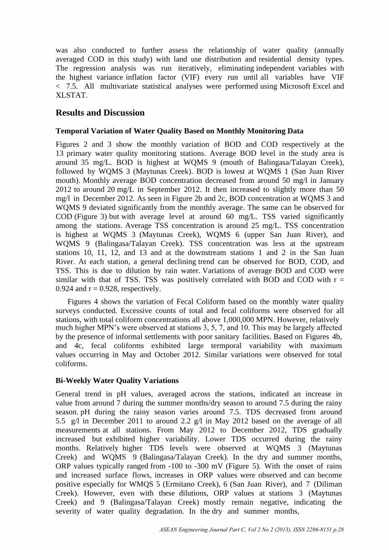
Figures 4 shows the variation of Fecal Coliform based on the monthly water quality
surveys conducted. Excessive counts of total and fecal coliforms were observed for all
stations, with total coliform concentrations all above 1,000,000 MPN. However, relatively
ASEAN Engineering Journal Part C, Vol 2 No 2 (2013), ISSN 2286-8151 p.28
much higher MPN’s were observed at stations 3, 5, 7, and 10. This may be largely affected
by the presence of informal settlements with poor sanitary facilities. Based on Figures 4b,
and 4c, fecal coliforms exhibited large termporal variability with maximum
values occurring in May and October 2012. Similar variations were observed for total
coliforms.
Bi-Weekly Water Quality Variations
General trend in pH values, averaged across the stations, indicated an increase in
value from around 7 during the summer months/dry season to around 7.5 during the rainy
season. pH during the rainy season varies around 7.5. TDS decreased from around
5.5 g/l in December 2011 to around 2.2 g/l in May 2012 based on the average of all
measurements at all stations. From May 2012 to December 2012, TDS gradually
increased but exhibited higher variability. Lower TDS occurred during the rainy
months. Relatively higher TDS levels were observed at WQMS 3 (Maytunas
Creek) and WQMS 9 (Balingasa/Talayan Creek). In the dry and summer months,
ORP values typically ranged from -100 to -300 mV (Figure 5). With the onset of rains
and increased surface flows, increases in ORP values were observed and can become
positive especially for WMQS 5 (Ermitano Creek), 6 (San Juan River), and 7 (Diliman
Creek). However, even with these dilutions, ORP values at stations 3 (Maytunas
Creek) and 9 (Balingasa/Talayan Creek) mostly remain negative, indicating the
severity of water quality degradation. In the dry and summer months,
average DO levels were extremely low at around 1 mg/l. During the rainy months,
DO concentration typically improves with the average reaching 3 mg/l, partly due to
increased flow.
ASEAN Engineering Journal Part C, Vol 2 No 2 (2013), ISSN 2286-8151 p.29
Figure 2. Monthly BOD variation at the 13 primary WQMSs: (a) station-to-station
variation, (b) temporal variation for WQMS 1-7, and (c) temporal variation for WQMS
8-13. Average shown is the average of all data per station or per month.
Figure 3. Monthly COD variation at the 13 primary WQMSs: (a) station-to-station
variation, (b) temporal variation for WQMS 1-7, and (c) temporal variation for WQMS
8-13. Average shown is the average of all data per station or per month.
ASEAN Engineering Journal Part C, Vol 2 No 2 (2013), ISSN 2286-8151 p.30
Figure 4. Monthly variation of fecal coliform concentration at the 13 primary WQMSs: (a)
station-to-station variation, (b) temporal variation for WQMS 1-7, and (c) temporal
variation for WQMS 8-13. Average shown is the average of all data per station or per
month.
ASEAN Engineering Journal Part C, Vol 2 No 2 (2013), ISSN 2286-8151 p.31
Figure 5. Temporal variation of ORP at the 13 primary WQMSs based on bi-weekly in situ
water quality surveys
Ranking and Class Grouping of Rivers and Creeks
Table 2 shows the ranking of rivers and creeks based on average COD and BOD
values obtained for the 13 primary WQMS. Balingasa/Talayan Creek and Maytunas Creek
are the worst in water quality with COD greater than 80 mg/L and BOD around 50 mg/
L. ORP were all negative (i.e., reducing condition), except for WQMS 13 (Pasong
Tamo River) where the average was positive.
Table 2. Ranking of Rivers/Creeks Based on Average COD and Average BOD WQMS River/Creek ORP CODaverage BODaverage Rank
9 Balingasa/Talayan Creek -146.6 100.3 51.5 1
3 Maytunas Creek -168.1 88.6 49.6 2
7 Diliman Creek -26.2 71.8 37.8 3
12 Dario River -43.2 70.7 37.3 4
6 San Juan River -114.5 66.8 37.1 5
11 San Francisco River -61.1 66.1 34.9 6
8 San Juan River -107.4 65.0 34.6 7
10 Mariblo Creek -9.0 61.8 33.3 8
13 Pasong Tamo River 23.4 61.7 33.4 9
5 Ermitano Creek -81.3 60.7 32.8 10
4 San Juan River -108.4 58.8 31.9 11
2 San Juan River -139.6 47.1 27.4 12
ASEAN Engineering Journal Part C, Vol 2 No 2 (2013), ISSN 2286-8151 p.32
1 San Juan River -117.0 42.6 24.1 13
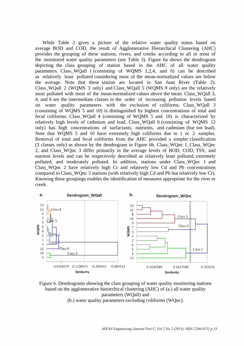
While Table 2 gives a picture of the relative water quality status based on
average BOD and COD, the result of Agglomerative Hierarchical Clustering (AHC)
provides the grouping of these stations, rivers, and creeks according to all or most of
the monitored water quality parameters (see Table 3). Figure 6a shows the dendrogram
depicting the class grouping of station based in the AHC of all water quality
parameters. Class_WQall 1 (consisting of WQMS 1,2,4, and 6) can be described
as relatively least polluted considering most of the mean-normalized values are below
the average. Note that these station are located in San Juan River (Table 2).
Class_WQall 2 (WQMS 3 only) and Class_WQall 5 (WQMS 9 only) are the relatively
most polluted with most of the mean-normalized values above the mean. Class_WQall 3,
4, and 6 are the intermediate classes in the order of increasing pollution levels based
on water quality parameters with the exclusion of coliforms. Class_WQall 3
(consisting of WQMS 5 and 10) is distinguished by highest concentrations of total and
fecal coliforms. Class_WQall 4 (consisting of WQMS 5 and 10) is characterized by
relatively high levels of cadmium and lead. Class_WQall 6 (consisting of WQMS 12
only) has high concentrations of surfactants, nutrients, and cadmium (but not lead).
Note that WQMS 5 and 10 have extremely high coliforms due to 1 or 2 samples.
Removal of total and fecal coliforms from the AHC provided a simpler classification
(3 classes only) as shown by the dendrogram in Figure 6b. Class_WQnc 1, Class_WQnc
2, and Class_WQnc 3 differ primarily in the average levels of BOD, COD, TSS, and
nutrient levels and can be respectively described as relatively least polluted, extremely
polluted, and moderately polluted. In addition, stations under Class_WQnc 1 and
Class_WQnc 2 have relatively high Cr and relatively low Cd and Pb concentrations
compared to Class_WQnc 3 stations (with relatively high Cd and Pb but relatively low Cr).
Knowing these groupings enables the identification of measures appropriate for the river or
creek.
Figure 6. Dendrograms showing the class grouping of water quality monitoring stations
based on the agglomerative hierarchical clustering (AHC) of (a.) all water quality
parameters (WQall) and
(b.) water quality parameters excluding coliforms (WQnc).
ASEAN Engineering Journal Part C, Vol 2 No 2 (2013), ISSN 2286-8151 p.33
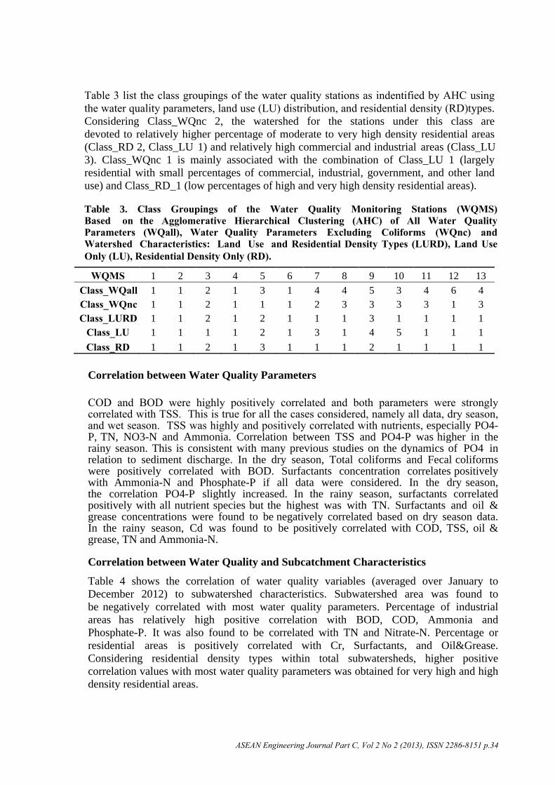
Table 3 list the class groupings of the water quality stations as indentified by AHC using the water quality parameters, land use (LU) distribution, and residential density (RD)types. Considering Class_WQnc 2, the watershed for the stations under this class are
devoted to relatively higher percentage of moderate to very high density residential areas
(Class_RD 2, Class_LU 1) and relatively high commercial and industrial areas (Class_LU
3). Class_WQnc 1 is mainly associated with the combination of Class_LU 1 (largely
residential with small percentages of commercial, industrial, government, and other land
use) and Class_RD_1 (low percentages of high and very high density residential areas).
Table 3. Class Groupings of the Water Quality Monitoring Stations (WQMS) Based on the Agglomerative Hierarchical Clustering (AHC) of All Water Quality Parameters (WQall), Water Quality Parameters Excluding Coliforms (WQnc) and Watershed Characteristics: Land Use and Residential Density Types (LURD), Land Use Only (LU), Residential Density Only (RD).
WQMS 1 2 3 4 5 6 7 8 9 10 11 12 13
Class_WQall 1 1 2 1 3 1 4 4 5 3 4 6 4
Class_WQnc 1 1 2 1 1 1 2 3 3 3 3 1 3
Class_LURD 1 1 2 1 2 1 1 1 3 1 1 1 1
Class_LU 1 1 1 1 2 1 3 1 4 5 1 1 1
Class_RD 1 1 2 1 3 1 1 1 2 1 1 1 1
Correlation between Water Quality Parameters
COD and BOD were highly positively correlated and both parameters were strongly correlated with TSS. This is true for all the cases considered, namely all data, dry season, and wet season. TSS was highly and positively correlated with nutrients, especially PO4-P, TN, NO3-N and Ammonia. Correlation between TSS and PO4-P was higher in the rainy season. This is consistent with many previous studies on the dynamics of PO4 in relation to sediment discharge. In the dry season, Total coliforms and Fecal coliforms were positively correlated with BOD. Surfactants concentration correlates positively with Ammonia-N and Phosphate-P if all data were considered. In the dry season, the correlation PO4-P slightly increased. In the rainy season, surfactants correlated positively with all nutrient species but the highest was with TN. Surfactants and oil & grease concentrations were found to be negatively correlated based on dry season data. In the rainy season, Cd was found to be positively correlated with COD, TSS, oil & grease, TN and Ammonia-N.
Correlation between Water Quality and Subcatchment Characteristics
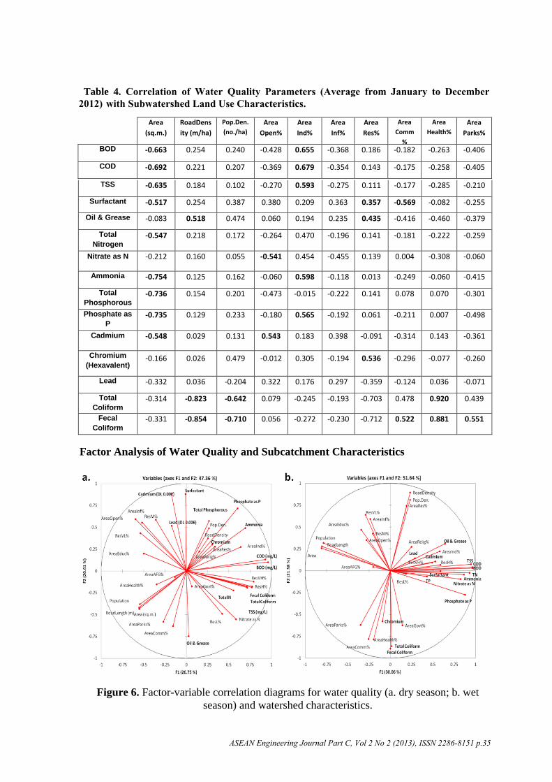
Table 4 shows the correlation of water quality variables (averaged over January to
December 2012) to subwatershed characteristics. Subwatershed area was found to
be negatively correlated with most water quality parameters. Percentage of industrial
areas has relatively high positive correlation with BOD, COD, Ammonia and
Phosphate-P. It was also found to be correlated with TN and Nitrate-N. Percentage or
residential areas is positively correlated with Cr, Surfactants, and Oil&Grease.
Considering residential density types within total subwatersheds, higher positive
correlation values with most water quality parameters was obtained for very high and high
density residential areas.
ASEAN Engineering Journal Part C, Vol 2 No 2 (2013), ISSN 2286-8151 p.34
Table 4. Correlation of Water Quality Parameters (Average from January to December 2012) with Subwatershed Land Use Characteristics.
Figure 7. Factor correlation diagram for water quality (dry season) and watershed
characteristics for stations grouped under (a) Class_WQnc 1 and (b) Class_WQnc 3.
The factor-variable correlation diagrams showing the association of water quality with watershed variables during dry and wet seasons are given in Figure 6. The first two factors F1 and F2 accounted for about 47% (dry season) and 51% (wet season) of the total data variability. In the dry season, COD and BOD were associated with industrial areas (AreaInd%) and high density residential areas. Fecal Coliforms and Total Coliforms were closely related to high (ResH%) to very high (ResVH%) residential density areas in the dry season. However, this relationship was lost during the rainy season. TSS, BOD, COD, Fecal Coliform, Total Coliform and nutrients remain closely related to percentages of areas devoted to industries and high density residential areas.
Figure 7 shows the factor-variable correlation diagrams showing the association of water
quality with watershed variables during dry wet season for the Class_WQnc 1 ((Figure 7b)
and Class_WQnc 3 (Figure 7b) resulting from agglomerative cluster analysis. Note that
applying the total percent variability represented by the factors were much higher. For the
Class_WQnc 1 stations, TP and surfactants were closely associated with AreaRes% and
ResVH%. Cd was associated with AreaInd% to certain extent. On factor D2, TN and
coliforms can be related to AreaInf%. For the relatively more polluted stations under
Class_WQnc 3, AreaInd% were closely associated with BOD, COD, TSS, and PO4-P. TN
and NO3-N were associated with ResVH%.
Multiple Linear Regression Models for COD
The relationships of COD with land use distribution (including roads) and with residential density type distribution are given respectively by the following multiple linear regression
Figure 8. Standardized coefficients of the multiple linear regression models for COD using (a.) land use distribution variables and (b.) residual density types variables.
Regression model 1 has an R2 = 0.821 and Adjusted R
2 = 0.731 while regression model 2
has an R2 = 0.436 and Adjusted R
2 = 0.323. This indicates the relative importance of land
use distribution in controlling COD levels compared to residential densities. Figure 8
shows the standardized coefficients of these regression models. Based on the regression
model (Equation 1), higher percentage of areas devoted to industries (AreaInd%) and occupied by informal settlements (AreaInf%) will translate to higher COD concentrations.
Based on the analysis of water samples before and after informal settlements, COD can be
increased by at least 10 mg/L after the water passed through these settlements.
AreaInd% was relatively the more important contributor of COD than AreaInf% based on
the standardized model coefficients. Reductions in COD are associated with more open
areas (AreaOpen%) and roads (Roadlength) as these are not major sources of COD. Note
that the residential area variable (AreaRes%) did not contribute significant explanatory
power to the model.
ASEAN Engineering Journal Part C, Vol 2 No 2 (2013), ISSN 2286-8151 p.37
However, it is known the residential areas are also contributors of COD. Based on the
regression analysis of COD and residential density types, ResH% or high percentage of
high density residential areas (i.e., 66-90 dwellings per hectare) was associated with higher
COD in the case of San Juan River and its tributaries. On the other hand, ResL% or very
low residential density (i.e., 1-5 dwellings per hectare) was associated with lower COD.
ResH% was relatively a stronger predictor of COD compared to ResL% (Equation 2, Figure 8b).
CONCLUSIONS
The water quality variations observed by means of measurement and monitoring following
different schemes indicated the severe degradation of water quality brought about
by pollutants from a variety of sources such as dense residential areas, industrial zones,
and commercial establishments. Temporal variations of various water quality
parameters including COD and BOD pointed to the dilution effect of increased runoff
due to rains. However, concentrations typically revert back to summer levels in the
succeeding weeks and months, pointing to large volumes of wastewater being
discharged from houses and establishments. Areas dominated with high density
industrial and residential uses have much lower surface water quality as exemplified
by the Balingasa Creek and Maytunas Creek. Variations in water quality were
observed along the creeks and rivers, with relatively higher values near point and areal
sources (e.g, informal settlements). The results of multivariate statistical techniques
confirmed these observations and provided a more detailed picture of the intra-water
quality relationships and the associations between watershed characteristics and
water quality measures. Cluster analysis has identified distinct groups of stations
(and therefore rivers and creeks) for which appropriate river-specific water quality
improvement measures must be formulated. Factor analysis pinpointed relevant land
uses and residential density types likely controlling the observed spatial variation of
water quality. The relative explanatory power of these factors can be assessed using
multiple linear regression as shown in the case of COD.
ACKNOWLEDGEMENT
This research was funded through the Pasig River Tributary Survey and Assessment Study (PRTSAS) of the Pasig River Rehabilitation Commission (PRRC) and the University of the Philippines Training Center for Applied Geodesy and Photogrammetry (UP-TCAGP), College of Engineering, University of the Philippines Diliman. The authors are thankful for the support of the UP DOST Engineering Research and Development for
Technology (ERDT) Program.
REFERENCES
[1] E.L. Thackstorn, and K.D. Young, “Housing density and bacterial loading in urban streams,” Journal of Environmental Engineering, pp. 1177-1180, 1990.
[2] H. Chang, “Spatial and temporal variations of water quality in the Han river and its tributaries, Seoul, Korea,” Water, Air, and Soil Pollution, Vol. 161, pp. 267-284, 1993-2002, 2005.
[3] J.E. Whitlock, D.T. Jones, and V.J. Harwood, “Identification of the sources of fecal coliforms in an urban watershed using antibiotic resistance analysis,” Water Research, Vol. 36, pp. 4273-4282, 2002.
[4] S. Shrestha, and F. Kazama, “Assessment of surface water quality using multivariate statistical techniques: A case study of the Fuji river basin, Japan,” Environmental Modelling and Software, Vol. 22, pp. 464-465, 2007.
ASEAN Engineering Journal Part C, Vol 2 No 2 (2013), ISSN 2286-8151 p.38
[5] T.G. Kaz, M.B. Arain, M.K. Jamali, N. Jalbani, H.I. Afridi, R.A. Sarfraz, J.A. Baig, and A.Q. Shah, “Assessment of water quality of polluted lake using multivariate statistical techniques: A case study,” Ecotoxicology and Environmental Safety, Vol. 72, pp. 301-309, 2009.
[6] K.P. Singh, A. Malik, D. Mohan, and S. Sinha, “Multivariate statistical techniques for the evaluation of spatial and temporal variations in water quality of the Gomti River (India) – A case study,” Water Research, Vol. 38, pp. 3980-3992, 2004.
[7] K.P. Singh, A. Malik, and S. Simha, “Water quality assessment and apportionment of pollution sources of Gomti river (India) using multivariate statistical techniques – A case study,” Analytica Chimica Acta, Vol. 538, pp.355-274, 2005.
[8] H. Chang, “Spatial analysis of water quality trends in the Han river basin, South Korea,” Water Research, Vol. 42, pp. 3285-3304, 2008.
ASEAN Engineering Journal Part C, Vol 2 No 2 (2013), ISSN 2286-8151 p.40


![files/Chamber/[Clarinet_Institute] Salamon... · Piano Sean Salarnon 10 Variations on a Theme: 'Brâul" ... Variations on a Theme Variations on a Theme Lento Variations on a Theme](https://static.documents.pub/doc/80x56/5b3431957f8b9a7e4b8bd2d8/clarinetinstitute-salamon-piano-sean-salarnon-10-variations-on-a-theme.jpg)
![VARIATIONS GOLDBERG [ARIA et 30 variations] · Title: VARIATIONS GOLDBERG [ARIA et 30 variations] Author: Bach, Johann Sebastian - Arranger: Montreuille, Pierre - Publisher: Montreuille,](https://static.documents.pub/doc/80x56/610885d0028fe95f64358299/variations-goldberg-aria-et-30-variations-title-variations-goldberg-aria-et.jpg)


