Asset backed securities: Risks, Ratings and Quantitative ... · PDF fileRisks, Ratings and...

Asset backed securities:

Risks, Ratings and Quantitative Modelling

December 2, 2009

Henrik Jonsson1 and Wim Schoutens2

EURANDOM Report 2009 - 50

1Postdoctoral Research Fellow, EURANDOM, Eindhoven, The Netherlands. E-mail: [email protected] Professor, Department of Mathematics, K.U.Leuven, Leuven, Belgium. E-mail: [email protected]

Abstract

Asset backed securities (ABSs) are structured finance products backed by pools of as-sets and are created through a securitisation process. The risks in asset backed securities,such as, credit risk, prepayment risk, market risks, operational risk, and legal risks, are di-rectly connected with the asset pool and the structuring of the securities. The assessmentof structured finance products is an assessment of these risks and how well the structuremitigates them. This procedure is partly based on quantitative models for the defaults andprepayments of the assets in the pool. In the present report we look at the risks presentin ABSs, present a collection of different default and prepayment models and describe twomajor rating agencies methodologies for assessing and rating ABSs. The topics covered inthe report are illustrated by case studies.

Acknolwledgement:The presented study is part of the research project “Quantitative analysis and analytical methodsto price securitisation deals”, sponsored by the European Investment Bank via the universityresearch sponsorship programme EIBURS. The authors acknowledge the intellectual supportfrom the participants of the previously mentioned project.

Project participants:Marcella Bellucci, Financial Engineering and Advisory Services, EIB, Luxembourg;Guido Bichisao, Head of Financial Engineering and Advisory Services, EIB, Luxembourg (EIBproject tutor);Henrik Jonsson, EURANDOM, The Netherlands (EURANDOM EIBURS research fellow);Luke Mellor, Creative Capital Partners, Sweden;Wim Schoutens, Katholieke Universiteit Leuven, Belgium (EURANDOM EIBURS project su-pervisor);Karsten Sundermann, Financial Engineering and Advisory Services, EIB, Luxembourg;Geert van Damme, Katholieke Universiteit Leuven, Belgium.

i

Contents

1 Introduction 1

2 Introduction to asset-backed securities 12.1 Key securitisation parties . . . . . . . . . . . . . . . . . . . . . . . . . . . . . . . 32.2 Structural characteristics . . . . . . . . . . . . . . . . . . . . . . . . . . . . . . . 32.3 Priority of payments . . . . . . . . . . . . . . . . . . . . . . . . . . . . . . . . . . 42.4 Loss allocation . . . . . . . . . . . . . . . . . . . . . . . . . . . . . . . . . . . . . 52.5 Credit enhancement . . . . . . . . . . . . . . . . . . . . . . . . . . . . . . . . . . 52.6 Basic risks . . . . . . . . . . . . . . . . . . . . . . . . . . . . . . . . . . . . . . . . 62.7 Triggers . . . . . . . . . . . . . . . . . . . . . . . . . . . . . . . . . . . . . . . . . 102.8 Rating . . . . . . . . . . . . . . . . . . . . . . . . . . . . . . . . . . . . . . . . . . 10

3 Cash flow modelling 113.1 Asset behaviour . . . . . . . . . . . . . . . . . . . . . . . . . . . . . . . . . . . . . 113.2 Structural features . . . . . . . . . . . . . . . . . . . . . . . . . . . . . . . . . . . 123.3 Revolving structures . . . . . . . . . . . . . . . . . . . . . . . . . . . . . . . . . . 12

4 Modelling defaults and prepayments 134.1 Deterministic default models . . . . . . . . . . . . . . . . . . . . . . . . . . . . . 13

4.1.1 Conditional default rate . . . . . . . . . . . . . . . . . . . . . . . . . . . . 134.1.2 Default vector approach . . . . . . . . . . . . . . . . . . . . . . . . . . . . 154.1.3 Logistic default model . . . . . . . . . . . . . . . . . . . . . . . . . . . . . 16

4.2 Stochastic default models . . . . . . . . . . . . . . . . . . . . . . . . . . . . . . . 184.2.1 Levy portfolio default model . . . . . . . . . . . . . . . . . . . . . . . . . 184.2.2 Normal one-factor default model . . . . . . . . . . . . . . . . . . . . . . . 204.2.3 Generic one-factor Levy default model . . . . . . . . . . . . . . . . . . . . 22

4.3 Deterministic prepayment models . . . . . . . . . . . . . . . . . . . . . . . . . . . 234.3.1 Conditional Prepayment Rate . . . . . . . . . . . . . . . . . . . . . . . . . 234.3.2 The PSA benchmark . . . . . . . . . . . . . . . . . . . . . . . . . . . . . . 244.3.3 A generalised CPR model . . . . . . . . . . . . . . . . . . . . . . . . . . . 25

4.4 Stochastic prepayment models . . . . . . . . . . . . . . . . . . . . . . . . . . . . . 264.4.1 Levy portfolio prepayment model . . . . . . . . . . . . . . . . . . . . . . . 264.4.2 Normal one-factor prepayment model . . . . . . . . . . . . . . . . . . . . 26

5 Rating agencies methodologies 285.1 Moody’s . . . . . . . . . . . . . . . . . . . . . . . . . . . . . . . . . . . . . . . . . 28

5.1.1 Non-Granular portfolios . . . . . . . . . . . . . . . . . . . . . . . . . . . . 285.1.2 Granular portfolios . . . . . . . . . . . . . . . . . . . . . . . . . . . . . . . 29

5.2 Standard and Poor’s . . . . . . . . . . . . . . . . . . . . . . . . . . . . . . . . . . 325.2.1 Credit quality of defaulted assets . . . . . . . . . . . . . . . . . . . . . . . 325.2.2 Cash flow modelling . . . . . . . . . . . . . . . . . . . . . . . . . . . . . . 34

5.3 Conclusions . . . . . . . . . . . . . . . . . . . . . . . . . . . . . . . . . . . . . . . 37

ii

6 Case studies 386.1 A two note structure . . . . . . . . . . . . . . . . . . . . . . . . . . . . . . . . . . 38

6.1.1 Cash flow modelling . . . . . . . . . . . . . . . . . . . . . . . . . . . . . . 406.1.2 Numerical results . . . . . . . . . . . . . . . . . . . . . . . . . . . . . . . . 43

6.2 Geldilux TS 2005 S.A. . . . . . . . . . . . . . . . . . . . . . . . . . . . . . . . . . 456.2.1 Structural features . . . . . . . . . . . . . . . . . . . . . . . . . . . . . . . 456.2.2 The Loan Portfolio . . . . . . . . . . . . . . . . . . . . . . . . . . . . . . . 496.2.3 Risks . . . . . . . . . . . . . . . . . . . . . . . . . . . . . . . . . . . . . . . 506.2.4 Performance . . . . . . . . . . . . . . . . . . . . . . . . . . . . . . . . . . 526.2.5 Summary . . . . . . . . . . . . . . . . . . . . . . . . . . . . . . . . . . . . 53

7 Summary 55

iii

February 8, 2010 ABS: Risks, Ratings and Quantitative Modelling

1 Introduction

The research project “Quantitative analysis and analytical methods to price securitisation deals”,sponsored by the European Investment Bank via the university research sponsorship programmeEIBURS, aims at conducting advanced research related to rating, pricing and risk managementof Asset-Backed Securities (ABSs). The analysis of existing default and prepayment models andthe development of new, more advanced default and prepayment models is one objective of theproject. Another objective is to achieve a better understanding of the major rating agenciesmethodologies and models for rating asset-backed securities, and the underlying assumptions andthe limitations in their methodologies and models. The analysis of a number of case studies willbe an integral part of the project. Finally, we aim to study the default and prepayment modelsinfluence on key characteristics of the asset-backed securities and also investigate the parametersensitivity and robustness of these key characteristics. The deliverables of the project are:

• Default and prepayment models: overview of standard models and new models;

• Rating agencies models and methods: summary of the agencies methodology to rate ABSs;

• Cash flow modelling: general comments on the most common features in ABS cash flows;

• Case studies: a number of existing ABS deals will be analysed and the default and pre-payment models will be tested on these deals;

• Sensitivity analysis: parameter sensitivity and robustness of key characteristics of ABSs(weighted average life, expected loss, rating, value).

A major contribution of the project will be the annually organisation of a workshop/conferencewith the aim to gather speakers and participants from both industry and academia, with ex-pertise in securitisation, asset-backed securities and related fields, to discuss the assessment andhandling of ABSs and what lessons that have been learned from the recent financial crisis. Topicsto be covered include: cash flow modelling; modelling of defaults and prepayments; data sourcesfor different securities; rating agency methodologies; risk management of ABSs; valuation; andsensitivity analysis.

The results and knowledge attained throughout the first half of the project is summarisedin the present report. The outline of the text is as follows. In Section 2, a short introduction toasset-backed securities is given. Cashflow modelling of ABS deals are divided into two parts: themodelling of the cash collections from the asset pool and the distribution of the collections to thenote holders. This is discussed in Section 3. The modelling of the cash collections from the assetpool depends heavily on default and prepayment models. A collection of default and prepaymentmodels are presented in Section 4. Rating agencies methodologies for rating ABS are discussedin Section 5. Section 6 presents case studies of ABS deals. The report is summarised in Section7.

2 Introduction to asset-backed securities

Asset-Backed Securities (ABSs) are structured finance products backed by pools of assets. ABSsare created through a securitisation process, where assets are pooled together and the liabilitiesbacked by these assets are tranched such that the ABSs have different seniority and risk-returnprofiles. The Bank for International Settlements defined structured finance through the followingcharacterisation (BIS (2005), p. 5):

1


• Pooling of assets;

• Tranching of liabilities that are backed by these collateral assets;

• De-linking of the credit risk of the collateral pool from the credit risk of the originator,usually through the use of a finite-lived, standalone financing vehicle.

Asset classes

The asset pools can be made up of almost any type of assets, ranging from common automobileloans, student loans and credit cards to more esoteric cash flows such as royalty payments(“Bowie bonds”). A few typical asset classes are listed in Table 1.

Auto leases Auto loansCommercial mortgages Residential mortgagesStudent loans Credit cardsHome equity loans Manufactured housing loansSME loans Entertainment royalties

Table 1: Some typical ABS asset classes.

In this project we have performed case study analysis of SME loans ABSs.There are several ways to distinguish between structured finance products according to their

collateral asset classes: cash flow vs. synthetic; existing assets vs. future flows; corporate relatedvs. consumer related.

• Cash flow: The interest and principal payments generated by the assets are passed throughto the notes. Typically there is a legal transfer of the assets.

• Synthetic: Only the credit risk of the assets are passed on to the investors through creditderivatives. There is no legal transfer of the underlying assets.

• Existing assets: The asset pool consists of existing assets, e.g., loan receivables, withalready existing cash flows.

• Future flows: Securitisation of expected cash flows of assets that will be created in thefuture, e.g., airline ticket revenues and pipeline utilisation fees.

• Corporate related: e.g., commercial mortgages, auto and equipment leases, trade receiv-ables;

• Consumer related: e.g., automobile loans, residential mortgages, credit cards, home equityloans, student loans.

Although it is possible to call all types of securities created through securitisation assetbacked securities it seems to be common to make a few distinctions. It is common to refer to se-curities backed by mortgages as mortgage backed securities (MBSs) and furthermore distinguishbetween residential mortgages backed securities (RMBS) and commercial mortgages backedsecurities (CMBS). Collateralised debt obligations (CDOs) are commonly viewed as a sepa-rate structured finance product group, with two subcategories: corporate related assets (loans,bonds, and/or credit default swaps) and resecuritisation assets (ABS CDOs, CDO-squared). Inthe corporate related CDOs can two sub-classes be distinguished: collateralised loan obligations(CLO) and collateralised bond obligations (CBO).

2


2.1 Key securitisation parties

The following parties are key players in securitisation:

• Originator(s): institution(s) originating the pooled assets;

• Issuer/Arranger: Sets up the structure and tranches the liabilities, sell the liabilities toinvestors and buys the assets from the originator using the proceeds of the sale. The Issueris a finite-lived, standalone, bankruptcy remote entity referred to as a special purposevehicle (SPV) or special purpose entity (SPE);

• Servicer: collects payments from the asset pool and distribute the available funds to theliabilities. The servicer is also responsible for the monitoring of the pool performance:handling delinquencies, defaults and recoveries. The servicer plays an important role inthe structure. The deal has an exposure to the servicer’s credit quality; any negative eventsthat affect the servicer could influence the performance and rating of the ABS. We notethat the originator can be the servicer, which in such case makes the structure exposed tothe originator’s credit quality despite the de-linking of the assets from the originator.

• Investors: invests in the liabilities;

• Trustee: supervises the distribution of available funds to the investors and monitors thatthe contracting parties comply to the documentation;

• Rating Agencies: Provide ratings on the issued securities. The rating agencies have amore or less direct influence on the structuring process because the rating is based notonly on the credit quality of the asset pool but also on the structural features of the deal.Moreover, the securities created through the tranching are typically created with specificrating levels in mind, making it important for the issuer to have an iterative dialogue withthe rating agencies during the structuring process. We point here to the potential dangercaused by this interaction. Because of the negotiation process a tranche rating, say ’AAA’,will be just on the edge of ’AAA’, i.e., it satisfies the minimal requirements for the ’AAA’rating without extra cushion.

• Third-parties: A number of other counterparties can be involved in a structured financedeal, for example, financial guarantors, interest and currency swap counterparties, andcredit and liquidity providers.

2.2 Structural characteristics

There are many different structural characteristics in the ABS universe. We mention here twobasic structures, amortising and revolving, which refer to the reduction of the pool’s aggregatedoutstanding principal amount.

Each collection period the aggregated outstanding principal of the assets can be reducedby scheduled repayments, unscheduled prepayments and defaults. To keep the structure fullycollateralized, either the notes have to be redeemed or new assets have to be added to the pool.

In an amortising structure, the notes should be redeemed according to the relevant priority ofpayments with an amount equal to the note redemption amount. The note redemption amountis commonly calculated as the sum of the principal collections from scheduled repayments andunscheduled prepayments over the collection period. Sometimes the recoveries of defaultedloans are added to the note redemption amount. Another alternative, instead of adding the

3


recoveries to the redemption amount, is to add the total outstanding principal amount of theloans defaulting in the collection period to the note redemption amount (see Loss allocation).

In a revolving structure, the Issuer purchases new assets to be added to the pool to keep thestructure fully collateralized. During the revolving period the Issuer may purchase additionalassets offered by the Originator, however these additional assets must meet certain eligibilitycriteria. The eligibility criteria are there to prevent the credit quality of the asset pool todeteriorate. The revolving period is most often followed by an amortisation period duringwhich the structure behaves as an amortising structure. The replenishment amount, the amountavailable to purchase new assets, is calculated in a similar way as the note redemption amount.

2.3 Priority of payments

The allocation of interest and principal collections from the asset pool to the transaction partiesis described by the priority of payments (or waterfall). The transaction parties that keeps thestructure functioning (originator, servicer, and issuer) have the highest priorities. After thesesenior fees and expenses, the interest payments on the notes could appear followed by poolreplenishment or note redemption, but other sequences are also possible.

Waterfalls can be classified either as combined waterfalls or as separate waterfalls. In acombined waterfall, all cash collections from the asset pool are combined into available fundsand the allocation is described in a single waterfall. There is, thus, no distinction made betweeninterest collections and principal collections. However, in a separate waterfall, interest collectionsand principal collections are kept separated and distributed according to an interest waterfall anda principal waterfall, respectively. This implies that the available amount for note redemptionor asset replenishment is limited to the principal cashflows.

A revolving structure can have a revolving waterfall, which is valid as long as replenishmentis allowed, followed by an amortising waterfall.

In an amortising structure, principal is allocated either pro rata or sequential. Pro rataallocation means a proportional allocation of the note redemption amount, such that the re-demption amount due to each note is an amount proportional to the note’s fraction of the totaloutstanding principal amount of the notes on the closing date.

Using sequential allocation means that the most senior class of notes is redeemed first, beforeany other notes are redeemed. After the most senior note is redeemed, the next note in rank isredeemed, and so on. That is, principal is allocated in order of seniority.

It is important to understand that “pro rata” and “sequential” refer to the allocation of thenote redemption amount, that is, the amounts to due to be paid to each class of notes. It is notdescribing the amounts actually being paid to the notes, which is controlled by the priority ofpayments and depends on the amount of available funds at the respectively level of the waterfall.

One more important term in connection with the priority of payments is pari passu, whichmeans that two or more parties have equal right to payments.

Example

Assume a structure with two classes of note, A and B, and the following simple waterfall:

1. Servicing fees;

2. Class A Interest;

3. Class B Interest;

4


4. Class A Principal;

5. Class B Principal;

6. Reserve account reimbursement;

7. Residual Payment.

In the above waterfall Class A Notes principal payments are ranked senior to Class B Notesprincipal payments. Assume that the principal payments to Class A Notes and Class B Notesare paid pari passu instead. Then Class A Notes and Class B Notes have equal rights to theavailable funds after level 3, and level 4 and 5 in the waterfall become effectively one level.Similarly, we can also assume that class A and class B interest payments are allocated pro rataand paid pari passu.

A more detailed description of the waterfall is given in Section 6.1.1.

2.4 Loss allocation

At defaults in the asset pool, the aggregate outstanding principal amount of the pool is reducedby the defaulted assets outstanding principal amount. There are basically two different ways todistribute these losses in the pool to the note investors: either direct or indirect. In a structurewhere losses are directly allocated to the note investors, the losses are allocated according toreverse order of seniority, which means that the most subordinated notes are first sufferingreduction in principal amount. This affects the subordinated note investors directly in twoways: loss of invested capital and a reduction of the coupon payments, since the coupon is basedon the note’s outstanding principal balance.

On the other hand, as already mentioned above in the description of structural character-istics, an amount equal to the principal balance of defaulted assets can be added to the noteredemption amount in an amortising structure to make sure that the asset side and the liabilityside is at par. In a revolving structure, this amount is added to the replenishment amountinstead. In either case, the defaulted principal amount to be added is taken from the excessspread (see Credit enhancement subsection below).

In an amortising structure with sequential allocation of principal, this method will reduce thecoupon payments to the senior note investors while the subordinated notes continue to collectcoupons based on the full principal amount (as long as there is enough available funds at thatlevel in the priority of payments). Any potential principal losses are not recognised until thefinal maturity of the notes.

2.5 Credit enhancement

Credit enhancements are techniques used to improve the credit quality of a bond and can beprovided both internally as externally.

The internal credit enhancement is provided by the originator or from within the deal struc-ture and can be achieved through several different methods: subordination, reserve fund, excessspread, over-collateralisation. The subordination structure is the main internal credit enhance-ment. Through the tranching of the liabilities a subordination structure is created and a priorityof payments (the waterfall) is setup, controlling the allocation of the cashflows from the assetpool to the securities in order of seniority.

Over-collateralisation means that the total nominal value of the assets in the collateral poolis greater than the total nominal value of the asset backed securities issued, or that the assets

5


are sold with a discount. Over-collateralisation creates a cushion which absorbs the initial lossesin the pool.

The excess spread is the difference between the interest and revenues collected from theassets and the senior expenses (for example, issuer expenses and servicer fees) and interest onthe notes paid during a month.

Another internal credit enhancement is a reserve fund, which could provide cash to coverinterest or principal shortfalls. The reserve fund is usually a percentage of the initial or out-standing aggregate principal amount of the notes (or assets). The reserve fund can be fundedat closing by proceeds and reimbursed via the waterfall.

When a third party, not directly involved in the securitisation process, is providing guaranteeson an asset backed security we speak about an external credit enhancement. This could be, forexample, an insurance company or a monoline insurer providing a surety bond. The financialguarantor guarantees timely payment of interest and timely or ultimate payment of principalto the notes. The guaranteed securities are typically given the same rating as the insurer.External credit enhancement introduces counterparty risk since the asset backed security nowrelies on the credit quality of the guarantor. Common monoline insurers are Ambac AssuranceCorporation, Financial Guaranty Insurance Company (FGIC), Financial Security Assurance(FSA) and MBIA, with the in the press well documented credit risks and its consequences (see,for example, KBC’s exposure to MBIA).

2.6 Basic risks

Due to the complex nature of securitisation deals there are many types of risks that have to betaken into account. The risks arise from the collateral pool, the structuring of the liabilities, thestructural features of the deal and the counterparties in the deal.

The main types of risks are credit risk, prepayment risk, market risks, reinvestment risk,liquidity risk, counterparty risk, operational risk and legal risk.

Credit Risk

Beginning with credit risk, this type of risk originates from both the collateral pool and thestructural features of the deal. That is, both from the losses generated in the asset pool andhow these losses are mitigated in the structure.

Defaults in the collateral pool results in loss of principal and interest. These losses aretransferred to the investors and allocated to the notes, usually in reverse order of seniorityeither directly or indirectly, as described in Section 2.4.

In the analysis of the credit risks, it is very important to understand the underlying assetsin the collateral pool. Key risk factors to take into account when analyzing the deal are:

• asset class(-es) and characteristics: asset types, payment terms, collateral and collaterali-sation, seasoning and remaining term;

• diversification: geographical, sector and borrower;

• asset granularity: number and diversification of the assets;

• asset homogeneity or heterogeneity;

An important step in assessing the deal is to understand what kind of assets the collateralpool consists of and what the purpose of these assets are. Does the collateral pool consist

6


of short term loans to small and medium size enterprizes where the purpose of the loans areworking capital, liquidity and import financing, or do we have in the pool residential mortgages?The asset types and purpose of the assets will influence the overall behavior of the pool andthe ABS. If the pool consists of loan receivables, the loan type and type of collateral is ofinterest for determining the loss given default or recovery. Loans can be of unsecured, partiallysecured and secured type, and the collateral can be real estates, inventories, deposits, etc. Thecollateralisation level of a pool can be used for the recovery assumption.

A few borrowers that stands for a significant part of the outstanding principal amount inthe pool can signal a higher or lower credit risk than if the pool consisted of a homogeneousborrower concentration. The same is true also for geographical and sector concentrations.

The granularity of the pool will have an impact on the behavior of the pool and thus theABS, and also on the choice of methodology and models to assess the ABS. If there are manyassets in the pool it can be sufficient to use a top-down approach modeling the defaults andprepayments on a portfolio level, while for a non-granular portfolio a bottom-up approach,modeling each individual asset in the pool, can be preferable. From a computational point ofview, a bottom-up approach can be hard to implement if the portfolio is granular. (Moody’s, forexample, are using two different methods: factor models for non-granular portfolios and NormalInverse default distribution and Moody’s ABSROMTM for granular, see Section 5.1.)

Prepayment Risk

Prepayment is the event that a borrower prepays the loan prior to the scheduled repaymentdate. Prepayment takes place when the borrower can benefit from it, for example, when theborrower can refinance the loan to a lower interest rate at another lender.

Prepayments result in loss of future interest collections because the loan is paid back pre-maturely and can be harmful to the securities, specially for long term securities.

A second, and maybe more important consequence of prepayments, is the influence of un-scheduled prepayment of principal that will be distributed among the securities according to thepriority of payments, reducing the outstanding principal amount, and thereby affecting theirweighted average life. If an investor is concerned about a shortening of the term we speak aboutcontraction risk and the opposite would be the extension risk, the risk that the weighted averagelife of the security is extended.

In some circumstances, it will be borrowers with good credit quality that prepay and thepool credit quality will deteriorate as a result. Other circumstances will lead to the oppositesituation.

Market Risk

The market risks can be divided into: cross currency risk and interest rate risk.The collateral pool may consist of assets denominated in one or several currencies different

from the liabilities, thus the cash flow from the collateral pool has to be exchanged to theliabilities’ currency, which implies an exposure to exchange rates. This risk can be hedged usingcurrency swaps.

The interest rate risk can be either basis risk or interest rate term structure risk. Basis riskoriginates from the fact that the assets and the liabilities may be indexed to different benchmarkindexes. In a scenario where there is an increase in the liability benchmark index that is notfollowed by an increase in the collateral benchmark index there might be a lack of interestcollections from the collateral pool, that is, interest shortfall.

7


The interest rate term structure risk arise from a mismatch in fixed interest collections fromthe collateral pool and floating interest payments on the liability side, or vice versa.

The basis risk and the term structure risk can be hedge with interest rate swaps.Currency and interest hedge agreements introduce counterparty risk (to the swap counter-

party), discussed later on in this section.

Reinvestment Risk

There exists a risk that the portfolio credit quality deteriorates over time if the portfolio isreplenished during a revolving period. For example, the new assets put into the pool cangenerate lower interest collections, or shorter remaining term, or will influence the diversification(geographical, sector and borrower) in the pool, which potentially increases the credit risk profile.

These risks can partly be handled through eligibility criteria to be compiled by the newreplenished assets such that the quality and characteristics of the initial pool are maintained.The eligibility criteria are typically regarding diversification and granularity: regional, sector andborrower concentrations; and portfolio characteristics such as the weighted average remainingterm and the weighted average interest rate of the portfolio.

Moody’s reports that a downward portfolio quality migration has been observed in assetbacked securities with collateral pools consisting of loans to small and medium size enterprizeswhere no efficient criteria were used (see Moody’s (2007c)).

A second common feature in replenishable transactions is a set of early amortisation triggerscreated to stop replenishment in case of serious delinquencies or defaults event. These triggersare commonly defined in such a way that replenishment is stopped and the notes are amortizedwhen the cumulative delinquency rate or cumulative default rate breaches a certain level. Moreabout performance triggers follow later.

Liquidity Risk

Liquidity risk refers to the timing mismatches between the cashflows generated in the asset pooland the cashflows to be paid to the liabilities. The cashflows can be either interest, principal orboth. The timing mismatches can occur due to maturity mismatches, i.e., a mismatch betweenscheduled amortisation of assets and the scheduled note redemptions, to rising number of delin-quencies, or because of delays in transferring money within the transaction. For interest ratesthere can be a mismatch between interest payment dates and periodicity of the collateral pooland interest payments to the liabilities.

Counterparty Risk

As already mentioned the servicer is a key party in the structure and if there is a negative eventaffecting the servicer’s ability to perform the cash collections from the asset pool, distribute thecash to the investors and handling delinquencies and defaults, the whole structure is put underpressure. Cashflow disruption due to servicer default must be viewed as a very severe event,especially in markets where a replacement servicer may be hard to find. Even if a replacementservicer can be found relatively easy, the time it will take for the new servicer to start performingwill be crucial.

Standard and Poor’s consider scenarios where the servicer may be unwilling or unable toperform its duties and a replacement servicer has to be found when rating a structured financetransaction. Factors that may influence the likelihood of a replacement servicer’s availabilityand willingness to accept the assignment are: ”... the sufficiency of the servicing fee to attract

8


a substitute servicer, the seniority of the servicing fee in the transaction’s payment waterfall,the availability of alternative servicers in the sector or region, and specific characteristics of theassets and servicing platform that may hinder an orderly transition of servicing functions toanother party.”3

Originator default can cause severe problems to a transaction where replenishment is allowed,since new assets cannot be put into the collateral pool.

Counterparty risk arises also from third-parties involved in the transaction, for example,interest rate and currency swap counterparties, financial guarantors and liquidity or credit sup-port facilities. The termination of a interest rate swap agreement, for example, may expose theissuer to the risk that the amounts received from the asset pool might not be enough for theissuer to meet its obligations in respect of interest and principal payments due under the notes.The failure of a financial guarantor to fulfill its obligations will directly affect the guaranteednote. The downgrade of a financial guarantor will have an direct impact on the structure, whichhas been well documented in the past years.

To mitigate counterparty risks, structural features, such as, rating downgrade triggers, col-lateralisation remedies, and counterparty replacement, can be present in the structure to (moreor less) de-link the counterparty credit risk from the credit risk of the transaction.

The rating agencies analyse the nature of the counterparty risk exposure by reviewing boththe counterparty’s credit rating and the structural features incorporated in the transaction. Therating agencies analyses are based on counterparty criteria frameworks detailing the key criteriato be fulfilled by the counterparty and the structure.4

Operational Risk

This refers partly to reinvestment risk, liquidity risk and counterparty risk, which was alreadydiscussed earlier. However, operational risk also includes the origination and servicing of the as-sets and the handling of delinquencies, defaults and recoveries by the originator and/or servicer.

The rating agencies conducts a review of the servicer’s procedures for, among others, collect-ing asset payments, handling delinquencies, disposing collateral, and providing investor reports.5

The originator’s underwriting standard might change over time and one way to detect the im-pact of such changes is by analysing trends in historical delinquency and default data.6 Moody’sremarks that the underwriting and servicing standards typically have a large impact on cumu-lative default rates and by comparing historical data received from two originators active inthe same market over a similar period can be a good way to assess the underwriting standardof originators: “Differences in the historical data between two originators subject to the samemacro-economic and regional situation may be a good indicator of the underwriting (e.g. riskappetite) and servicing standards of the two originators.”7

Legal Risks

The key legal risks are associated with the transfer of the assets from the originator to the issuerand the bankruptcy remoteness of the issuer. The transfer of the assets from the originator tothe issuer must be of such a kind that an originator insolvency or bankruptcy does not impair

3Standard and Poor’s (2007b) p. 4.4See Standard and Poor’s (2007a), Standard and Poor’s (2008a), Standard and Poor’s (2009c), and Moody’s

(2007b).5Moody’s (2007a) and Standard and Poor’s (2007b)6Moody’s (2005b) p. 8.7Moody’s (2009a) p. 7.

9


the issuer’s rights to control the assets and the cash proceeds generated by the asset pool. Thistransfer of the assets is typically done through a “true sale”.

The bankruptcy remoteness of the issuer depends on the corporate, bankruptcy and securi-tisation laws of the relevant legal jurisdiction.

2.7 Triggers

Triggers are used to modify the operation of the deal, for example: the ending of replenishmentand start of amortisation prior to the end date of the revolving period (early amortisationtriggers); changes to the priority of payments such that principal redemption of senior notes rankhigher than interest payments to subordinated notes (acceleration triggers); pro rata principalpayment is changed to sequential payment (acceleration triggers); or that interest on juniornotes are deferred to allow for a faster redemption of senior notes (interest deferral triggers).

Triggers can be divided into two groups: quantitative and qualitative. Example of quanti-tative triggers are cumulative delinquencies, default and loss rates triggers. In these cases thetrigger is hit if the observed quantity is above a certain level. This level can be time dependent,allowing for the trigger level to increase over time. Qualitative triggers refers to, for example,rating downgrade of servicer, swap counterparty, or another counterparties and the failure toreplace the affected transaction party within a certain time frame.

2.8 Rating

A rating is an assessment of either expected loss or probability of default.Moody’s ratings of ABSs are an expected loss assessment, which incorporates assessments of

both the likelihood of default and the severity of loss, given default. That is, the rating is basedon the probability weighted loss to the note investor. Moody’s makes the following definition ofstructured finance long-term ratings:

“Moody’s ratings on long-term structured finance obligations primarily address the expectedcredit loss an investor might incur on or before the legal final maturity of such obligations vis-a-vis a defined promise. As such, these ratings incorporate Moody’s assessment of the defaultprobability and loss severity of the obligations. They are calibrated to Moody’s CorporateScale. Such obligations generally have an original maturity of one year or more, unless explicitlynoted. Moody’s credit ratings address only the credit risks associated with the obligations;other non-credit risks have not been addressed, but may have a significant effect on the yield toinvestors.”8

With the probability of default approach the rating assess the likelihood of full and timelypayment of interest and the ultimate payment of principal no later than the legal final maturitydate. This is the approach taken by Standard and Poor’s and they make the following statementconcerning their issue credit rating definition:

“It takes into consideration the creditworthiness of guarantors, insurers, or other formsof credit enhancement on the obligation and takes into account the currency in which theobligation is denominated. The opinion evaluates the obligor’s capacity and willingness to meetits financial commitments as they come due, and may assess terms, such as collateral securityand subordination, which could affect ultimate payment in the event of default.”9

8see Rating Definitions, Structured Finance Long-Term Ratings on www.moodys.com.9Standard and Poor’s (2009d), p.3.

10


3 Cash flow modelling

The modelling of the cash flows in an ABS deal consists of two parts: the modelling of the cashcollections from the asset pool and the distribution of the collections to the note holders andother transaction parties.

The first step is to model the cash collections from the asset pool, which depends on thebehaviour of the pooled assets. This can be done in two ways: with a top-down approach,modelling the aggregate pool behaviour; or with a bottom-up approach modelling each individualloan. For the top-down approach one assumes that the pool is homogeneous, that is, each assetbehaves as the average representative of the assets in the pool (a so called representative lineanalysis or repline analysis). For the bottom-up approach one can chose to use either therepresentative line analysis or to model each individual loan (so called loan level analysis). Ifa top-down approach is chosen, the modeller has to choose between modelling defaulted andprepaid assets or defaulted and prepaid principal amounts, i.e., to count assets or money units.

On the liability side one has to model the waterfall, that is, the distribution of the cashcollections to the note holders, the issuer, the servicer and other transaction parties.

In this section we make some general comments on the cash flow modelling of ABS deals.The case studies presented later in this report will highlight the issues discussed here.

3.1 Asset behaviour

The assets in the pool can be categorised as performing, delinquent, defaulted, repaid andprepaid. A performing asset is an asset that pays interest and principal in time during acollection period, i.e. the asset is current. An asset that is in arrears with one or severalinterest and/or principal payments is delinquent. A delinquent asset can be cured, i.e. become aperforming asset again, or it can become a defaulted asset. Defaulted assets goes into a recoveryprocedure and after a time lag a portion of the principal balance of the defaulted assets arerecovered. A defaulted asset is never cured, it is once and for all removed from the pool. Whenan asset is fully amortised according to its amortisation schedule, the asset is repaid. Finally,an asset is prepaid if it is fully amortised prior to its amortisation schedule.

The cash collections from the asset pool consist of interest collections and principal collections(both scheduled repayments, unscheduled prepayments and recoveries). There are two parts ofthe modelling of the cash collections from the asset pool. Firstly, the modelling of performingassets, based on asset characteristics such as initial principal balance, amortisation scheme,interest rate and payment frequency and remaining term. Secondly, the modelling of the assetsbecoming delinquent, defaulted and prepaid, based on assumptions about the delinquency rates,default rates and prepayment rates together with recovery rates and recovery lags.

The characteristics of the assets in the pool are described in the Offering Circular and asummary can usually be found in the rating agencies pre-sale or new issue reports. The aggre-gate pool characteristics described are the total number of assets in the pool, current balance,weighted average remaining term, weighted average seasoning and weighted average coupon.The distribution of the assets in the pool by seasoning, remaining term, interest rate profile,interest payment frequency, principal payment frequency, geographical location, and industrysector are also given. Out of this pool description the analyst has to decide if to use a represen-tative line analysis assuming a homogeneous pool, to use a loan-level approach modelling theassets individually or take an approach in between modelling sub-pools of homogeneous assets.In this report we focus on large portfolios of assets, so the homogeneous portfolio approach (orhomogeneous sub-portfolios) is the one we have in mind.

11


For a homogeneous portfolio approach the average current balance, the weighted averageremaining term and the weighted average interest rate (or spread) of the assets are used asinput for the modelling of the performing assets. Assumptions on interest payment frequenciesand principal payment frequencies can be based on the information given in the offering circular.

Assets in the pool can have fixed or floating interest rates. A floating interest rate consistsof a base rate and a margin (or spread). The base rate is indexed to a reference rate and is resetperiodically. In case of floating rate assets, the weighted average margin (or spread) is given inthe offering circular. Fixed interest rates can sometimes also be divided into a base rate and amargin, but the base rate is fixed once and for all at the closing date of the loan receivable.

The scheduled repayments, or amortisations, of the assets contribute to the principal collec-tions and has to be modelled. Assets in the pool might amortise with certain payment frequency(monthly, quarterly, semi-annually, annually) or be of bullet type, paying back all principal atthe scheduled asset maturity, or any combination of these two (soft bullet).

The modelling of non-performing assets requires default and prepayment models which takesas input assumptions about delinquency, default, prepayment and recovery rates. These assump-tions have to be made on the basis of historical data, geographical distribution, obligor andindustry concentration, and on assumptions about the future economical environment. Severaldefault and prepayment models will be described in the next chapter.

We end this section with a remark about delinquencies. Delinquencies are usually importantfor a deal’s performance. A delinquent asset is usually defined as an asset that has failed tomake one or several payments (interest or principal) on scheduled payment dates. It is commonthat delinquencies are categorised in time buckets, for example, in 30+ (30-59), 60+ (60-89),90+ (90-119) and 120+ (120-) days overdue. However, the exact timing when a loan becomesdelinquent and the reporting method used by the servicer will be important for the classificationof an asset to be current or delinquent and also for determining the number of payments pastdue, see Moody’s (2000a).

3.2 Structural features

The key structural features discussed earlier in Section 2: structural characteristics, priority ofpayments, loss allocation, credit enhancements, and triggers, all have to be taken into accountwhen modelling the liability side of an ABS deal. So does the basic information on the noteslegal final maturity, payment dates, initial notional amounts, currency, and interest rates. Thestructural features of a deal are detailed in the offering circular.

In Section 6.1.1 a detailed description of the cash flow modelling in a transaction with twoclasses of notes is given.

3.3 Revolving structures

A revolving period adds an additional complexity to the modelling because new assets are addedto the pool. Typically each new subpool of assets should be handled individually, modellingdefaults and prepayments separately, because the assets in the different subpools will be indifferent stages of their default history. Default and prepayment rates for the new subpoolsmight also be assumed to be different for different subpools.

Assumptions about the characteristics of each new subpool of assets added to the pool haveto be made in view of interest rates, remaining term, seasoning, and interest and principalpayment frequencies. To do this, the pool characteristics at closing together with the eligibilitycriteria for new assets given in the offering circular can be of help.

12


4 Modelling defaults and prepayments

To be able to assess ABS deals one need to model the defaults and the prepayments in theunderlying asset pool. The models discussed here all refer to static pools.

We divide the default and prepayment models into two groups, deterministic and stochasticmodels. The deterministic models are simple models with no built in randomness, i.e., as soonas the model parameters are set the evolution of the defaults and prepayments are know forall future times. The stochastic models are more advanced, based on stochastic processes andprobability theory. By modelling the evolution of defaults and prepayments with stochasticprocesses we can achieve three objectives:

• Stochastic timing of defaults and prepayments;

• Stochastic monthly default and prepayments rates;

• Correlation: between defaults; between prepayments; and between defaults and prepay-ments.

We focus on the time interval between the issue (t = 0) of the ABS notes and the weightedaverage maturity of the underlying assets (T ).

The default curve, Pd(t), refers to the default term structure, i.e., the cumulative defaultrate at time t (expressed as percentage of the initial outstanding principal amount of the assetpool or the initial number of assets). By the default distribution, we mean the (probability)distribution of the cumulative default rate at time T .

The prepayment curve, Pp(t), refers to the prepayment term structure, i.e., the cumulativeprepayment rate at time t (expressed as percentage of the initial outstanding principal amountof the asset pool or the initial number of assets). By the prepayment distribution, we meanthe distribution of the cumulative prepayment rate at time T .

There are two approaches to choose between when modelling the defaults and prepayments:the top-down approach (portfolio-level models) and the bottom-up approach (loan-level models).In the top-down approach one model the cumulative default and prepayment rates of the port-folio. This is exactly what is done with the deterministic models we shall present later in thischapter. The bottom-up approach, on the other hand, one models the individual loans defaultand prepayment behavior. A number of loan level models are presented.

The choice of approach depends on several factors, such as, the number of loans in thereference pool.

4.1 Deterministic default models

4.1.1 Conditional default rate

The Conditional (or Constant) Default Rate (CDR) approach is the simplest way to use tointroduce defaults in a cash flow model. The CDR is a sequence of (constant) annual defaultrates applied to the outstanding pool balance in the beginning of the time period, hence themodel is conditional on the pool history and therefore called conditional. The CDR is an annualdefault rate that can be translated into a monthly rate by using the single-monthly mortality(SMM) rate:

SMM = 1 − (1 − CDR)1/12.

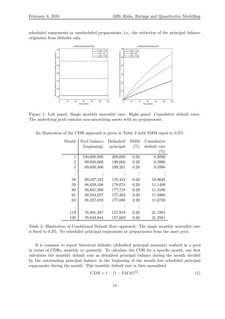
The SMM rates and the corresponding cumulative default rates for three values of CDR(2.5%, 5%, 7.5%) are shown in Figure 1. The CDRs were applied to a pool of asset with no

13


scheduled repayments or unscheduled prepayments, i.e., the reduction of the principal balanceoriginates from defaults only.

0 20 40 60 80 100 120

0.2

0.3

0.4

0.5

0.6

0.7

0.8

Time (months)

Mo

nth

ly d

efa

ult r

ate

(%

ou

tsta

nd

ing

po

ol b

ala

nce

)

Conditional Default Rate (CDR)

CDR = 2.5%CDR = 5%CDR = 7.5%

0 20 40 60 80 100 1200

10

20

30

40

50

60

Time (months)

Cu

mu

lative

De

fau

lt R

ate

(%

in

itia

l p

ort

folio

ba

lan

ce

)

Conditional Default Rate (CDR)

CDR = 2.5%CDR = 5%CDR = 7.5%

Figure 1: Left panel: Single monthly mortality rate. Right panel: Cumulative default rates.The underlying pool contains non-amortising assets with no prepayments.

An illustration of the CDR approach is given in Table 2 with SMM equal to 0.2%.

Month Pool balance Defaulted SMM Cumulative(beginning) principal (%) default rate

(%)

1 100,000,000 200,000 0.20 0.20002 99,800,000 199,600 0.20 0.39963 99,600,400 199,201 0.20 0.5988...

......

......

58 89,037,182 178,431 0.20 10.962859 88,859,108 178,074 0.20 11.140960 88,681,390 177,718 0.20 11.318661 88,504,027 177,363 0.20 11.496062 88,327,019 177,008 0.20 11.6730

......

......

...119 78,801,487 157,919 0.20 21.1985120 78,643,884 157,603 0.20 21.3561

Table 2: Illustration of Conditional Default Rate approach. The single monthly mortality rateis fixed to 0.2%. No scheduled principal repayments or prepayments from the asset pool.

It is common to report historical defaults (defaulted principal amounts) realised in a poolin terms of CDRs, monthly or quarterly. To calculate the CDR for a specific month, one firstcalculates the monthly default rate as defaulted principal balance during the month dividedby the outstanding principal balance in the beginning of the month less scheduled principalrepayments during the month. This monthly default rate is then annualised

CDR = 1 − (1 − SMM)12. (1)

14


Strengths and weaknesses

The CDR models is simple, easy to use and it is straight forward to introduce stresses on thedefault rate. It is even possible to use the CDR approach to generate default scenarios, byusing a probability distribution of the cumulative default rate. However, it is too simple, sinceit assumes that the default rate is constant over time.

4.1.2 Default vector approach

In the default vector approach, the total cumulative default rate is distributed over the life ofthe deal according to some rule. Hence, the timing of the defaults is modelled. Assume, forexample, that 24% of the initial outstanding principal amount is assumed to default over thelife of the deal, that is, the cumulative default rate is 24%. We could distribute these defaultsuniformly over the life of the deal, say 120 months, resulting in assuming that 0.2% of the initialprincipal balance defaults each month. If the initial principal balance is euro 100 million andwe assume 0.2% of the initial balance to default each month we have euro 200, 000 defaultingin every month. The first three months, five months in the middle and the last two months areshown in Table 3.

Note that this is not the same as the SMM given above in the Conditional Default Rateapproach, which is the percentage of the outstanding principal balance in the beginning of themonth that defaults. To illustrate the difference compare Table 2 (0.2% of the outstandingpool balance in the beginning of the month defaults) above with Table 3 (0.2% of the initialoutstanding pool balance defaults each month). The SMM in Table 3 is calculated as the ratioof defaulted principal (200, 000) and the outstanding portfolio balance at the beginning of themonth. Note that the SMM in Table 3 is increasing due to the fact that the outstanding portfoliobalance is decreasing while the defaulted principal amount is fixed.


(%)

1 100,000,000 200,000 0.2000 0.202 99,800,000 200,000 0.2004 0.403 99,600,000 200,000 0.2008 0.60...

......

......

58 88,600,000 200,000 0.2257 11.6059 88,400,000 200,000 0.2262 11.8060 88,200,000 200,000 0.2268 12.0061 88,000,000 200,000 0.2273 12.2062 87,800,000 200,000 0.2278 12.40

......

......

...119 76,400,000 200,000 0.2618 23.8120 76,200,000 200,000 0.2625 24.0

Table 3: Illustration of an uniformly distribution of the cumulative default rate (24% of theinitial pool balance) over 120 months, that is, each month 0.2% of the initial pool balance isassumed to default. No scheduled principal repayments or prepayments from the asset pool.

Of course many other default timing patterns are possible. Moody’s methodology to rate

15


granular portfolios is one such example, where default timing is based on historical data, seeSection 5.1. S&P’s apply this approach in its default stress scenarios in the cash flow analysis,see Section 5.2.


Easy to use and to introduce different default timing scenarios, for example, front-loaded or back-loaded. The approach can be used in combination with a scenario generator for the cumulativedefault rate.

4.1.3 Logistic default model

The Logistic default model is used for modelling the default curve, that is, the cumulative defaultrate’s evolution over time. Hence it can be viewed as an extension of the default vector approachwhere the default timing is given by a functional representation. In its most basic form, theLogistic default model has the following representation:

Pd(t) =a

(1 + be−c(t−t0)),

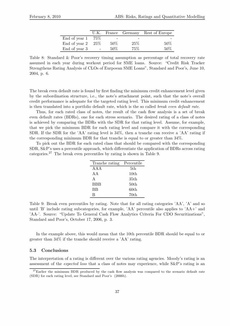
where a, b, c, t0 are positive constants and t ∈ [0, T ]. Parameter a is the asymptotic cumulativedefault rate; b is a curve adjustment or offset factor; c is a time constant (spreading factor); andt0 is the time point of maximum marginal credit loss. Note that the Logistic default curve hasto be normalised such that it starts at zero (initially no defaults in the pool) and Pd(T ) equalsthe expected cumulative default rate.

From the default curve, which represents the cumulative default rate over time, we can findthe marginal default curve, which describes the periodical default rate, by differentiating Pd(t).Figure 1 shows a sample of default curves (left panel) and the corresponding marginal defaultcurves (right panel) with time measured in months. Note that most of the default take place inthe middle of the deal’s life and that the marginal default curve is centered around month 60,which is due to our choice of t0. More front-loaded or back-loaded default curves can be createdby decreasing or increasing t0.

Table 4 illustrates the application of the Logistic default model to the same asset pool thatwas used in Table 3. The total cumulative default rate is 24% in both tables, however, thedistribution of the defaulted principal is very different. For the Logistic model, the defaultedprincipal amount (as well as the SMM) is low in the beginning, very high in the middle andthen decays in the second half of the time period. So the bulk of defaults occur in the middleof the deal’s life. This is of course due to our choice of t0 = 60. Something which is also evidentin Figure 2.

The model can be extended in several ways. Seasoning could be taken into account in themodel and the asymptotic cumulative default rate (a) can be divided into two factors, onesystemic factor and one idiosyncratic factor (see Raynes and Ruthledge (2003)).

The Logistic default model thus has (at least) four parameters that have to be estimated fromdata (see, for example, Raynes and Ruthledge (2003) for a discussion on parameter estimation).

Introducing randomness

The Logistic default model can easily be used to generate default scenarios. Assuming that wehave a default distribution at hand, for example, the log-normal distribution, describing thedistribution of the cumulative default rate at maturity T . We can then sample an expected

16


0 20 40 60 80 100 1200

0.1

0.2

0.3

0.4

0.5

0.6

0.7

t

Cu

mu

lative

de

fau

lt r

ate

(%

)

Logistic default curve (µ = 0.20 , σ = 10)

a = 0.1797a = 0.1628a = 0.1468

0 20 40 60 80 100 1200

0.002

0.004

0.006

0.008

0.01

0.012

0.014

0.016

0.018

t

Mo

nth

ly d

efa

ult r

ate

(%

)


a = 0.1797a = 0.1628a = 0.1468

Figure 2: Left panel: Sample of Logistic default curves (cumulative default rates). Right panel:Marginal default curves (monthly default rates). Parameter values: a is sampled from a log-normal distribution (with mean 20% and standard deviation 10%), b = 1, c = 0.1 and t0 = 60.


(%)

1 100,000,000 6,255 0.006255 0.0062552 99,993,745 6,909 0.006909 0.0131643 99,986,836 7,631 0.007632 0.020795...

......

......

58 89,795,500 593,540 0.660991 10.20450059 89,201,960 599,480 0.672048 10.79804060 88,602,480 602,480 0.679981 11.39752061 88,000,000 602,480 0.684636 12.00000062 87,397,520 599,480 0.685923 12.602480

......

......

...119 76,006,255 6,909 0.009089 23.993745120 76,000,000 6,255 0.008230 24.000000

Table 4: Illustration of an application of the Logistic default model. The cumulative defaultrate is assumed to be 24% of the initial pool balance. No scheduled principal repayments orprepayments from the asset pool. Parameter values: a = 0.2406, b = 1, c = 0.1 and t0 = 60.

cumulative default rates from the distribution and fit the ’a’ parameter such that Pd(T ) equalsthe expected cumulative default rate. Keeping all the other parameters constant. Figure 3shows a sample of Logistic default curves in the left panel, each curve has been generated froma cumulative default rate sampled from the log-normal distribution shown in the right panel.

17


0 20 40 60 80 100 1200

0.1

0.2

0.3

0.4

0.5

0.6

0.7

t

Cu

mu

lative

de

fau

lt r

ate

(%

)


a = 0.1797a = 0.1628a = 0.1468

0 1 2 3 4 5 60

0.1

0.2

0.3

0.4

0.5

0.6

0.7

0.8

0.9

1

X ∼

Lo

gN

(µ, σ

)

fX

Probability density of LogN(µ = 0.20 , σ = 0.10)

Figure 3: Left panel: Sample of Logistic default curves (cumulative default rates). Parametervalues: a is sampled from the log-normal distribution to the right, b = 1, c = 0.1 and t0 = 60.Right panel: Log-normal default distribution with mean 0.20 and standard deviation 0.10.


The model is attractive because the default curve has an explicit analytic expression. With thefour parameters (a, b, c, t0) many different transformations of the basic shape is possible, givingthe user the possibility to create different default scenarios. The model is also easy to implementinto a Monte Carlo scenario generator.

The evolutions of default rates under the Logistic default model has some important draw-backs: they are smooth, deterministic and static.

For the Logistic default model most defaults happen gradually and are a bit concentrated inthe middle of the life-time of the pool. The change of the default rates are smooth. The modelis, however, able of capturing dramatic changes of the monthly default rates.

Furthermore, the model is deterministic in the sense that once the expected cumulativedefault rate is fixed, there is no randomness in the model.

Finally, the defaults are modelled independently of prepayments.

4.2 Stochastic default models

As was discussed in the previous section the deterministic default models have limited possibil-ities to capture the stochastic nature of the phenomena they are set to model. In the presentsection we propose a number of models that incorporate the stylized features of defaults. Wemodel the evolution of defaults with stochastic processes.

4.2.1 Levy portfolio default model

The Levy portfolio default model models the cumulative default rate on portfolio level. Thedefault curve, i.e., the fraction of loans that have defaulted at time t, is given by:

Pd(t) = 1 − exp(−Xt),

where X = {Xt, t ≥ 0} is a stochastic process. Because we are modelling the cumulative defaultrate the default curve Pd(t) must be non-decreasing over time (since we assume that a defaulted

18


asset is not becoming cured). To achieve this we need to assume that X = {Xt, t ≥ 0} isnon-decreasing over time, since then exp(−Xt) is non-decreasing. Furthermore, assuming thatall assets in the pool are current (Pd(0) = 0) at the time of issue (t = 0) we need X0 = 0.Our choice of process comes from the family of stochastic processes called Levy process, moreprecisely the single-sided Levy processes. A single-sided Levy process is non-decreasing and theincrements are through jumps.

By using a stochastic process to “drive” the default curve, Pd(t) becomes a random variable,for all t > 0. In order to generate a default curve scenario, we must first draw a realization ofthe process X = {Xt, t ≥ 0}. Moreover, Pd(0) = 0, since we start the Levy process at zero:X0 = 0.

As an example, let us consider a default curve based on a Gamma process G = {Gt, t ≥ 0}with shape parameter a and scale parameter b. The increment from time 0 to time t of theGamma process, i.e., Gt − G0 = Gt (recall that G0 = 0) is a Gamma random variable withdistribution Gamma (at, b), for any t > 0. Consequently, the cumulative default rate at maturityfollows the law 1 − e−GT , where GT ∼ Gamma (aT, b). Using this result, the parameters a andb can be found by matching the expected value and the variance of the cumulative default rateunder the model to the mean and variance of the default distribution, that is, as the solution tothe following system of equations:

E[

1 − e−GT]

= µd;

Var[

1 − e−GT]

= σ2d,

(2)

for predetermined values of the mean µd and standard deviation σd of the default distribution.Explicit expressions for the left hand sides of (2) can be found, by noting that the expectedvalue and the variance can be written in terms of the characteristic function of the Gammadistribution.

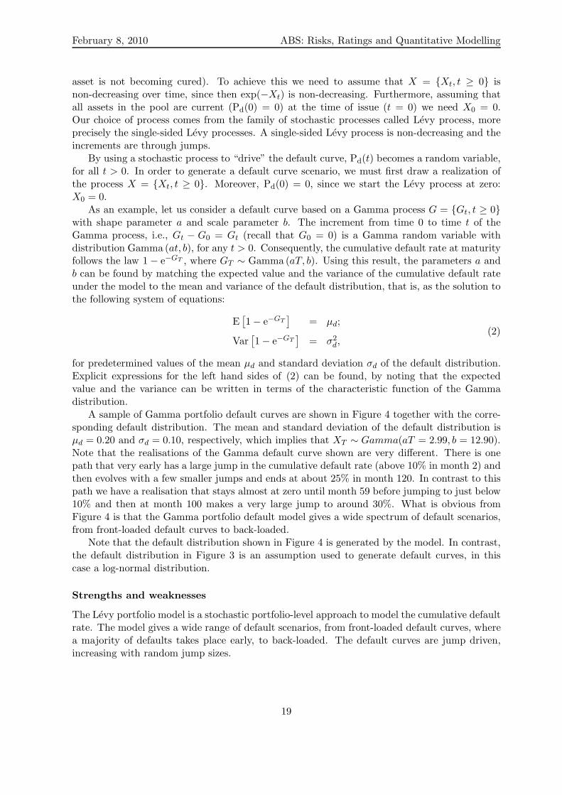
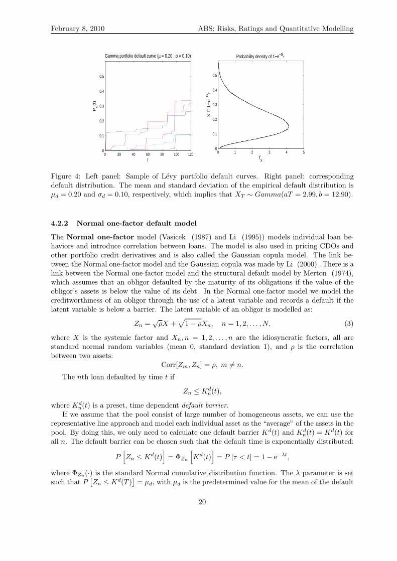
A sample of Gamma portfolio default curves are shown in Figure 4 together with the corre-sponding default distribution. The mean and standard deviation of the default distribution isµd = 0.20 and σd = 0.10, respectively, which implies that XT ∼ Gamma(aT = 2.99, b = 12.90).Note that the realisations of the Gamma default curve shown are very different. There is onepath that very early has a large jump in the cumulative default rate (above 10% in month 2) andthen evolves with a few smaller jumps and ends at about 25% in month 120. In contrast to thispath we have a realisation that stays almost at zero until month 59 before jumping to just below10% and then at month 100 makes a very large jump to around 30%. What is obvious fromFigure 4 is that the Gamma portfolio default model gives a wide spectrum of default scenarios,from front-loaded default curves to back-loaded.

Note that the default distribution shown in Figure 4 is generated by the model. In contrast,the default distribution in Figure 3 is an assumption used to generate default curves, in thiscase a log-normal distribution.


The Levy portfolio model is a stochastic portfolio-level approach to model the cumulative defaultrate. The model gives a wide range of default scenarios, from front-loaded default curves, wherea majority of defaults takes place early, to back-loaded. The default curves are jump driven,increasing with random jump sizes.

19


0 20 40 60 80 100 1200

0.1

0.2

0.3

0.4

0.5

t

Pd(t

)

Gamma portfolio default curve (µ = 0.20 , σ = 0.10)

0 1 2 3 4 50

0.1

0.2

0.3

0.4

0.5

X ∼

1−

e−

GT

fX

Probability density of 1−e−GT

Figure 4: Left panel: Sample of Levy portfolio default curves. Right panel: correspondingdefault distribution. The mean and standard deviation of the empirical default distribution isµd = 0.20 and σd = 0.10, respectively, which implies that XT ∼ Gamma(aT = 2.99, b = 12.90).

4.2.2 Normal one-factor default model

The Normal one-factor model (Vasicek (1987) and Li (1995)) models individual loan be-haviors and introduce correlation between loans. The model is also used in pricing CDOs andother portfolio credit derivatives and is also called the Gaussian copula model. The link be-tween the Normal one-factor model and the Gaussian copula was made by Li (2000). There is alink between the Normal one-factor model and the structural default model by Merton (1974),which assumes that an obligor defaulted by the maturity of its obligations if the value of theobligor’s assets is below the value of its debt. In the Normal one-factor model we model thecreditworthiness of an obligor through the use of a latent variable and records a default if thelatent variable is below a barrier. The latent variable of an obligor is modelled as:

Zn =√

ρX +√

1 − ρXn, n = 1, 2, . . . , N, (3)

where X is the systemic factor and Xn, n = 1, 2, . . . , n are the idiosyncratic factors, all arestandard normal random variables (mean 0, standard deviation 1), and ρ is the correlationbetween two assets:

Corr[Zm, Zn] = ρ, m 6= n.

The nth loan defaulted by time t if

Zn ≤ Kdn(t),

where Kdn(t) is a preset, time dependent default barrier.

If we assume that the pool consist of large number of homogeneous assets, we can use therepresentative line approach and model each individual asset as the “average” of the assets in thepool. By doing this, we only need to calculate one default barrier Kd(t) and Kd

n(t) = Kd(t) forall n. The default barrier can be chosen such that the default time is exponentially distributed:

P[

Zn ≤ Kd(t)]

= ΦZn

[

Kd(t)]

= P [τ < t] = 1 − e−λt,

where ΦZn(·) is the standard Normal cumulative distribution function. The λ parameter is setsuch that P

[

Zn ≤ Kd(T )]

= µd, with µd is the predetermined value for the mean of the default

20


distribution. Note that Kd(t) is non-decreasing in t, which implies that a defaulted loan staysdefaulted and cannot be cured.

The correlation parameter ρ is set such that the standard deviation of the model match thestandard deviation of the default distribution at time T , σd.

Given a sample of (correlated) standard Normal random variables Z = (Z1, Z2, ..., ZN ), thedefault curve is then given by

Pd(t;Z) =♯{

Zn ≤ Kd(t);n = 1, 2, ..., N}

N, t ≥ 0. (4)

In order to simulate default curves, one must thus first generate a sample of standard Normalrandom variables Zn satisfying (3), and then, at each (discrete) time t, count the number of Zi’sthat are less than or equal to the value of the default barrier Kd

t at that time.The left panel of Figure 5 shows five default curves, generated by the Normal one-factor model

(3) with ρ ≈ 0.121353, such that the mean and standard deviation of the default distributionare 0.20 and 0.10. We have assumed in this realisation that all assets have the same defaultbarrier. All curves start at zero and are fully stochastic, but unlike the Levy portfolio modelthe Normal one-factor default model does not include any jump dynamics. The correspondingdefault distribution is again shown in the right panel.

0 20 40 60 80 100 1200

0.1

0.2

0.3

0.4

0.5

t

Pd(t

)

Normal one−factor default curve (µ = 0.20 , σ = 0.10)

0 1 2 3 4 50

0.1

0.2

0.3

0.4

0.5

#{Z

i ≤ H

T}

f#{Z

i ≤ H

T}

Probability density of the cumulative default rate at time T (ρ = 0.12135)

Figure 5: Left panel: Sample of Normal one-factor default curves. Right panel: correspondingdefault distribution. The mean and standard deviation of the empirical default distribution isµd = 0.20 and σd = 0.10.

Just as for the Levy portfolio default model we would like to point out that the defaultdistribution is generated by the model, in contrast to the Logistic model. In Figure 5, anexample of a default distribution is shown.


The Normal one-factor model is a loan-level approach to modelling the cumulative portfoliodefault rate. In the loan-level approach one has the freedom to choose between assuming ahomogeneous or a heterogeneous portfolio. For a large portfolio with with quite homogeneousassets the representative line approach can be used, assuming that each of the assets in theportfolio behaves as the average asset. For a small heterogeneous portfolio it might be better tomodel the assets on an individual basis.

21


The Normal one-factor model can be used to model both the default and prepayment of anobligor, which will be evident in the section on prepayment modelling.

A known problem with the Normal one-factor model is that many joint defaults are veryunlikely. The underlying reason is the too light tail-behavior of the standard normal distribution(a large number of joint defaults will be caused by a very large negative common factor X).

4.2.3 Generic one-factor Levy default model

To introduce heavier tails one can use Generic one-factor Levy models (Albrecher et al(2006)) in which the latent variable of obligor i is of the form

Zn = Yρ + Y(n)1−ρ, n = 1, 2, . . . , N, (5)

where Yt and Y(n)t are Levy processes with the same underlying distribution L with distribution

function H1(x). Each Zn has by stationary and independent increment property the samedistribution L. If E[Y 2

1 ] < ∞, the correlation is again given by:

Corr[Zm, Zn] = ρ, m 6= n.

As for the Normal one-factor model, we again say that a borrower defaults at time t, if Zn

hits a predetermined barrier Kd(t) at that time, where Kd(t) satisfies

P[

Zn ≤ Kd(t)]

= 1 − e−λt, (6)

with λ determined as in the Normal one-factor model.As an example we use the Shifted-Gamma model where Y, Yn, n = 1, 2, . . . , n are independent

and identically distributed shifted Gamma processes

Y = {Yt = tµ − Gt : t ≥ 0},

where µ is a positive constant and Gt is a Gamma process with parameters a and b. Thus, thelatent variable of obligor n is of the form:

Zn = Yρ + Y(n)1−ρ = µ − (Gρ + G

(n)1−ρ), n = 1, 2, . . . , N. (7)

In order to simulate default curves, we first have to generate a sample of random variablesZ = (Z1, Z2, ..., ZN ) satisfying (5) and then, at each (discrete) time t, count the number of Zi’sthat are less than or equal to the value of the default barrier Kd(t) at that time. Hence, thedefault curve is given by

Pd(t;Z) =♯{

Zn ≤ Kd(t);n = 1, 2, ..., N}

N, t ≥ 0. (8)

The left panel of Figure 6 shows five default curves, generated by the Gamma one-factormodel (7) with (µ, a, b) = (1, 1, 1), and ρ ≈ 0.095408, such that the mean and standard deviationof the default distribution are 0.20 and 0.10. Again, all curves start at zero and are fullystochastic. The corresponding default distribution is shown in the right panel. Compared tothe previous three default models, the default distribution generated by the Gamma one-factormodel seems to be squeezed around µd and has a significantly larger kurtosis. Again we do nothave to assume a given default distribution, the default distribution will be generated by themodel.

22


It should also be mentioned that the latter default distribution has a rather heavy right tail(not shown in the graph), with a substantial probability mass at the 100 % default rate. Thiscan be explained by looking at the right-hand side of equation (7). Since both terms betweenbrackets are strictly positive and hence cannot compensate each other (unlike the Normal one-factor model), Zi is bounded from above by µ. Hence, starting with a large systematic riskfactor Y , things can only get worse, i.e. the term between the parentheses can only increaseand therefore Zi can only decrease, when adding the idiosyncratic risk factor Yi. This impliesthat when we have a substantially large common factor, it is more likely that all borrowers willdefault, than with the Normal one-factor model.

0 20 40 60 80 100 1200

0.05

0.1

0.15

0.2

0.25

t

Pd(t

)

Gamma 1−factor default curve (µ = 0.20 , σ = 0.10)

0 5 10 15 20 25 30 35 400

0.05

0.1

0.15

0.2

0.25

#{Z

i ≤ H

T}

f#{Z

i ≤ H

T}

Probability density of the cumulative default rate at time T (ρ = 0.09541)

Figure 6: Left panel: Sample of Gamma one-factor default curves. Right panel: correspondingdefault distribution. The mean and standard deviation of the empirical default distribution isµd = 0.20 and σd = 0.10.


The generic Levy one-factor model is a loan-level model, just as the Normal one-factor model,but with the freedom to choose the underlying probability distribution from a large set ofdistributions. The distributions are more heavy tailed than the normal distribution, that is,give a higher probability to large positive or negative values. A higher probability that thecommon factor is a large negative number gives higher probability to have many defaults.

4.3 Deterministic prepayment models

4.3.1 Conditional Prepayment Rate

The Conditional (or Constant) Prepayment Rate (CPR) model is a top-down approach. Itmodels the annual prepayment rate, which one applies to the outstanding pool balance thatremains at the end of the previous month, hence the name conditional prepayment rate model.The CPR is an annual prepayment rate, the corresponding monthly prepayment rate is givenby the single-monthly mortality rate (SMM) and the relation between the two is:

SMM = 1 − (1 − CPR)1/12.

23



The strength of the CPR model lies in it simplicity. It allows the user to easily introduce stresseson the prepayment rate.

A drawback of the CPR model is that the prepayment rate is constant over the life of thedeal, implying that the prepayments as measured in euro amounts are largest in the beginning ofthe deal’s life and then decreases. A more reasonable assumption about the prepayment behaviorof loans would be that prepayments ramp-up over an initial period, such that the prepaymentsare larger after the loans have seasoned.10

4.3.2 The PSA benchmark

The Public Securities Association (PSA) benchmark for 30-year mortgages11 is a model whichtries to model the seasoning behaviour of prepayments by including a ramp-up over an initialperiod. It models a monthly series of annual prepayment rates: starting with a CPR of 0.2% forthe first month after origination of the loans followed by a monthly increase of the CPR by anadditional 0.2% per annum for the next 30 months when it reaches 6% per year, and after thatstaying fixed at a 6% CPR for the remaining years. That is, the marginal prepayment curve(monthly fraction of prepayments) is of the form:

CPR(t) =

6%30 t , 0 ≤ t ≤ 30

6% , 30 < t ≤ 360,

t=1,2,...,360 months. Remember that this is annual prepayment rates. The single-monthlyprepayment rates are

SMM(t) = 1 − (1 − CPR(t))1/12.

Speed-up or slow-down of the PSA benchmark is possible:

• 50 PSA means one-half the CPR of the PSA benchmark prepayment rate;

• 200 PSA means two times the CPR of the PSA benchmark prepayment rate.


The possibility to speed-up or slow-down the prepayment speed is giving the model some flexi-bility.

The PSA benchmark is a deterministic model, with no randomness in the prepayment curve’sbehaviour. And it assumes that the prepayment rate is changing smoothly over time, it isimpossible to model dramatic changes in the prepayment rate of a short time interval, that is,to introduce the possibility that the prepayment rate suddenly jumps. Finally, under the PSAbenchmark the ramp-up of prepayments always takes place during the first 30 months and therate is after that constant.

10Discussed in Fabozzi and Kothari (2008) page 33.11The benchmark has been extended to other asset classes such as home equity loans and manufacturing housing,

with adjustments to fit the stylized features of those assets, Fabozzi and Kothari (2008).

24


4.3.3 A generalised CPR model

A generalisation of the PSA benchmark is to model the monthly prepayment rates with thesame functional form as the CPR above. That is, instead of assuming that CPR(t) has thefunctional form above, we assume now that SMM(t) can be described like that. The marginalprepayment curve (monthly fraction of prepayments) is described as follows:

pp(t) =

apt , 0 ≤ t ≤ t0p

apt0p , t0p < t ≤ T,

where ap is the single-monthly prepayment rate increase.The prepayment curve, i.e., the cumulative prepayment rate, is found by calculating the area

under the marginal prepayment curve:

Pp(t) =

ap

2 t2 , 0 ≤ t ≤ t0p

ap

2 t20p + apt0p(t − t0p) , t0p < t ≤ T

The model has two parameters:

• t0p: the time where one switches to a constant CPR (t0p = 30 months in PSA);

• Pp(T ): the cumulative prepayment rate at maturity. For example, Pp(T ) = 0.20 meansthat 20% of the initial portfolio have prepaid at maturity T . Can be sampled from aprepayment distribution.

Once the parameters are set, one can calculate the rate increase per month

ap =Pp(T )

t20p

2 + t0p(T − t0p).

Introducing randomness

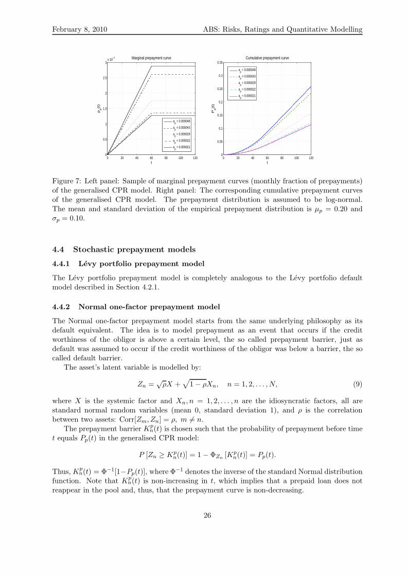
The generation of prepayment scenarios can easily be done with the generalised prepaymentmodel introduced above. Assuming that we have a prepayment distribution at hand, for example,the log-normal distribution, describing the distribution of the cumulative prepayment rate atmaturity T . We can then sample an expected cumulative prepayment rate from the distribution,and fit the ap parameter such that Pp(T ) equals the expected cumulative prepayment rate.Figure 7 shows a sample of marginal prepayment curves and the corresponding cumulativeprepayment curves.

Strengths and Weaknesses

The evolution of prepayment rates under the generalised CPR model is smooth and deterministic.The prepayment curve is smooth, no jumps are present, and it is completely determined oncet0p and Pp(T ) are chosen. Furthermore, after t0p the model assumes that the prepayment rateis constant.

25


0 20 40 60 80 100 1200

0.5

1

1.5

2

2.5

3x 10

−3

t

pp(t

)

Marginal prepayment curve

ap = 0.000048

ap = 0.000043

ap = 0.000029

ap = 0.000022

ap = 0.000021

0 20 40 60 80 100 1200

0.05

0.1

0.15

0.2

0.25

0.3

0.35

t

Pp(t

)

Cumulative prepayment curve

ap = 0.000048

ap = 0.000043

ap = 0.000029

ap = 0.000022

ap = 0.000021

Figure 7: Left panel: Sample of marginal prepayment curves (monthly fraction of prepayments)of the generalised CPR model. Right panel: The corresponding cumulative prepayment curvesof the generalised CPR model. The prepayment distribution is assumed to be log-normal.The mean and standard deviation of the empirical prepayment distribution is µp = 0.20 andσp = 0.10.

4.4 Stochastic prepayment models

4.4.1 Levy portfolio prepayment model

The Levy portfolio prepayment model is completely analogous to the Levy portfolio defaultmodel described in Section 4.2.1.

4.4.2 Normal one-factor prepayment model

The Normal one-factor prepayment model starts from the same underlying philosophy as itsdefault equivalent. The idea is to model prepayment as an event that occurs if the creditworthiness of the obligor is above a certain level, the so called prepayment barrier, just asdefault was assumed to occur if the credit worthiness of the obligor was below a barrier, the socalled default barrier.

The asset’s latent variable is modelled by:

Zn =√

ρX +√

1 − ρXn, n = 1, 2, . . . , N, (9)

where X is the systemic factor and Xn, n = 1, 2, . . . , n are the idiosyncratic factors, all arestandard normal random variables (mean 0, standard deviation 1), and ρ is the correlationbetween two assets: Corr[Zm, Zn] = ρ, m 6= n.

The prepayment barrier Kpn(t) is chosen such that the probability of prepayment before time

t equals Pp(t) in the generalised CPR model:

P [Zn ≥ Kpn(t)] = 1 − ΦZn [Kp

n(t)] = Pp(t).

Thus, Kpn(t) = Φ−1[1−Pp(t)], where Φ−1 denotes the inverse of the standard Normal distribution

function. Note that Kpn(t) is non-increasing in t, which implies that a prepaid loan does not

reappear in the pool and, thus, that the prepayment curve is non-decreasing.

26


0 10 20 30 40 50 60 70 80 90 100−6

−4

−2

0

2

4

6

t

Prepayment

Default

Loan 1

Loan 2

Loan 3

Prepayment barrier

Default barrier

Figure 8: Example of a default barrier and a prepayment barrier in a one-factor model.

Figure 8 shows how a prepayment barrier and a default barrier can be combined in anone-factor model.

The prepayment curve is defined as:

Pp(t;Z) =♯ {Zn ≥ Kp(t);n = 1, 2, ..., N}

N, t ≥ 0. (10)

0 20 40 60 80 100 1200

0.1

0.2

0.3

0.4

0.5

t

Pp(t

)

Normal 1−factor prepayment curve (µ = 0.20 , σ = 0.10)

0 0.5 1 1.5 2 2.5 3 3.5 4 4.50

0.1

0.2

0.3

0.4

0.5

#{Z

i ≥ H

T}

f#{Z

i ≥ H

T}

Probability density of the cumulative prepayment rate at time T (ρ = 0.12135)

Figure 9: Left panel: Sample of Normal one-factor prepayment curves. Right panel: Correspond-ing prepayment distribution. The mean and standard deviation of the empirical prepaymentdistribution is µp = 0.20 and σp = 0.10.

Comparing the prepayment curves in Figure 9 with the curves generated by the generalisedCPR model in the right panel of Figure 7, one can see that they are similar in shape due tothe fact that the prepayment barrier is chosen such that the probability of prepayment of anindividual obligor equals the cumulative prepayment rate given by the generalised CPR model.However, the prepayment curves generated by the Normal one-factor model are stochastic ascan be seen from the non-linear behaviour of the curves.

27


Note that the prepayment distribution is generated by the model. This is in contrast withthe prepayment distribution shown for the generalised CPR model in Figure 7 where we assumedthe log-normal distribution.


The evolution of the prepayment curve is stochastic, not deterministic. Furthermore, with theNormal one-factor model it is possible to model both default and prepayment of a single obligorat the same time.

See also comments on the Normal one-factor default model.

5 Rating agencies methodologies

The present section gives a summary of two of the major rating agencies quantitative method-ologies to provide ratings to ABSs, in particular to ABSs backed by SME loans.

5.1 Moody’s

In this section we focus on Moody’s approach to rating SME transactions, although the basicmethodologies is similar for other asset classes. As was already mentioned in Chapter 2, Moody’srating is an expected loss assessment, which incorporate the assessment of both the likelihood ofdefault and the severity of loss, given default. The quantitative rating is based on the results froma quantitative model, which calculates the Expected Loss and the Expected Weighted AverageLife of an ABS note. This quantitative rating is combined with a qualitative analysis, whichincludes an operational overview of the originator and the servicer and legal issues (transfer ofassets and bankruptcy), to derive a final rating (Moody’s (2001) and Moody’s (2007a)).

The quantitative rating methodology used depends on the size and granularity of the un-derlying SME portfolio. For small or non-granular portfolios, such as CDO’s, Moody’s takes abottom-up approach and use factor models (typically based on the Gaussian-copula approach,for example the Normal one-factor model presented previously) for the analysis. For granularportfolios Moody’s adopt a default distribution (Lognormal or Normal Inverse) approach, tomodel the cumulative default rate at the deal maturity. The factor models are implemented inMoody’s CDOROMTM and Moody’s STARFINDERTM (see Moody’s (2006b)); the granularapproach in Moody’s ABSROMTM (see Moody’s (2006a)).

In general, Moody’s classifies SME portfolios with more than 1, 000 assets and no majorconcentrations as ABS SME.12

General information guidelines describing the data that Moody’s would like to receive fromthe originator for SME securitisation transactions are given in Moody’s (2007a).

5.1.1 Non-Granular portfolios

For concentrated, heterogeneous pools the main tool for deriving a default distribution isMoody’s CDOROMTM . The portfolio default distribution will be directly derived from MonteCarlo simulations, which simulates the default of each individual asset based on a factor model

12To discriminate non-granular, granular and intermediate portfolios, Moody’s calculates the Effective Numberof Obligors, based on the Herfindahl index (see Moody’s (2007c).

28


as described previously in Section 4.2.2. The factor models used are typically based on onefactor:

Zn =√

ρcXc +√

1 − ρcXn,

or, on two factors:Zn =

√ρcXc +

√ρiXi +

√

1 − ρc − ρiXn,

where Xc is the common global factor, Xi is an industry factor, Xn, n = 1, 2, . . . , N is theindividual firm specific factor, and ρc and ρi is the global inter-industry and the sector specificintra-industry correlation assumptions, respectively, see Moody’s (2007d).

The input parameters in the model are the probability of default of each individual assetand the asset correlation. The individual default probability is typically derived from either (i)public ratings, (ii) credit estimates or (iii) a mapping between the originator’s internal ratingsystem and Moody’s rating scale. The correlation is derived from Moody’s corporate correlationframework adopted in global CDOs. However, Moody’s stresses the correlation parameters from3% to 6% depending on the specific characteristics of the portfolio, to account for a highergeographical concentration and industrial clustering typically present in SME pools.13

In contrast to the approach for granular portfolios described below, the default timing isdirectly generated in the factor models since the default of each individual asset is simulated.

In CDOROMTM the recovery rates are stochastic and assumed to be distributed accordingto a Beta distribution applied to each defaulted asset.14

To derive a rating, the present value of the loss for the note and the note’s weighted averagelife are calculated for each simulation run and the averages over all simulations are taken as esti-mates of the expected loss and the expected weighted average life. (A more detailed descriptionis given in the section on granular portfolios.)

The rating of the note is found from Moody’s Idealised Cumulative Expected Loss Table,which map the Expected Average Life and Expected Loss combination to a specific quantitativerating. An example of such a table is given in Moody’s (2000b).

5.1.2 Granular portfolios

For granular portfolios a default distribution for the total cumulative default rate (expressed asper cent of initial portfolio outstanding principal amount) over the life of the pool is assumed,typically a Normal Inverse15 distribution (previously Moody’s used the Lognormal distributionas standard, but this has changed (Moody’s (2007c))). The default distribution is characterisedby two parameters: the mean and the standard deviation, that has to be estimated. Moody’sestimates these parameters from historical static cohort data provided by the originator. Thisdata is typically given in a Static cumulative default rate table describing different cohorts (orvintages) of pools of loans and the cumulative default rate over a number of periods afterorigination. From this data estimates of the mean and standard deviation is derived. The basicmethodology of how to extrapolate, clean and adjust for seasoning is described in Moody’s(2005b). The parameter estimation based on historical cohort data is (almost) only applicableat the time the transaction is issued, because it is rarely that updated cohort data is madeavailable at a later stage after the closing date. To handle this problem Moody’s has developeda methodology to revise the default assumptions over the life of an ABS transaction (Moody’s

13Moody’s (2007c), p. 4.14Moody’s (2007c), p. 8.15The Normal Inverse distribution is an approximation of the default distribution if the Normal one-factor

model is used for a large homogeneous portfolio, see Appendix A and Moody’s (2003) and Moody’s (2007d).

29


(2008)). The method takes as input transaction specific performance data, such as delinquencyrates, historical periodic default or loss rates and historical portfolio redemption rates.

Based on the default distribution a set of Default Scenarios are derived and the scenarioprobability is given by the default distribution. The default scenarios are 0.00%, 0.10%, 0.20%, . . .and the scenario probability is the probability that the default rate falls between two consecutivedefault scenarios.16 Figure 10 illustrates the Normal Inverse distribution and the 20% defaultscenario with its associated probability.

0 20 40 60 80 1000

0.05

0.1

0.15

0.2

0.25

0.3

0.35

0.4

Default Rates (% initial portfolio balance defaulted)

Pro

babi

lity

(%)

Probability of 20% default rate

Figure 10: Illustration of a Normal Inverse default distribution. The 20% Default Scenarioand its associated probability is marked with a bar. The asset correlation was assumed to beρ = 20%, and the mean cumulative default rate 20%. The default barrier was estimated asdescribed in the section on the Normal one-factor default model.

To distribute the defaults over the life of the pool a Default Timing vector is defined. Foreach period, the corresponding element in the Default Timing vector is the percentage of thetotal cumulative default rate that will be applicable in that period. The Default Timing vectoris used to calculate the outstanding amount of the defaulted loans per period in each defaultscenario:

Defaulted Amount(period i, scenario s) = DefaultTiming (period i) × DefaultRate(scenario s)×Original PortfolioAmount.

The default timing is preferably derived from historical static cohort data on defaults (Moody’s(2007c)).

For granular portfolios the recovery rate is assumed to be stochastic with a Normal distri-bution and is applied on a portfolio basis.17 Historical recovery data provided by the originatoris used in order to determine the recovery rate. In ABSROMTM a Recovery Timing vector isused to specify the timing of the recoveries.

16Moody’s (2006a), p. 34.17Moody’s (2007c), p. 8. What is meant with “applied on a portfolio basis” is not clear. Using a Normal

distribution for the recovery rate implies that the recovery rate can become negative. However, Moody’s arguesthat by the Law of Large Numbers, if all LGDs are independent and identically distributed, the average LGDwill be almost equal to its expected value for high default rates, which implies that the right tail of the lossdistribution will not depend on the shape of the LGD distribution for each asset. See discussion in footnotes 30and 31 in Moody’s (2003), p. 18 and 19, respectively.

30


For the prepayments Moody’s assumes a fixed annual constant prepayment rate (CPR),which is estimated from the originator’s historical data.

To come to a rating Moody′s ABSROMTM calculates the Expected Average Life (or weightedaverage life) and the Expected Loss of the note (see Moody’s (2006a), p. 32-33). The ExpectedAverage Life of the note is given by:

Last Default Scenario∑

s=1st Default Scenario

Weighted Average Life(scenario s) × Probability(scenario s),

where Weighted Average Life(scenario s) is:

Legal Maturity Date∑

i=1st Period

Outstanding Note Amount(Period i, scenario s)

Original Note Amount × Number of Periods per Annum.

The expected loss is calculated as the sum-product of the probability of each default scenarioand the corresponding Relative Net Present Value-Loss. For each default scenario, the RelativeNet Present Value-Loss for a note is calculated by discounting the cashflows (both interest andprincipal) received on that note with a discount rate which is equal to the rate of that note andby comparing it to the initial outstanding amount on the note (Moody’s (2006a), p. 33):

Relative NPV Loss(Scenario s) =Nominal Initial Amount − NPV Cashflow(Scenario s)

Nominal Initial Amount.

The expected loss is then given by:

Expected Loss =Last Default Scenario

∑

s=1st Default Scenario

RelativeNPV Loss(Scenario s) · Probability(Scenario s).

For a fixed rate note the discount rate will be the promised coupon rate and for a floatingrate note it will be the realised benchmark rate plus the note’s margin.

The rating of the note is found from Moody’s Idealised Cumulative Expected Loss Table,which map the Expected Average Life and Expected Loss combination to a specific quantitativerating. An example of such a table is given in Moody’s (2000b).

V Scores and Parameter Sensitivity

Moody’s has recently introduced two changes to the way structured finance ratings are presented:V Scores and Parameter Sensitivities. Moody’s V Scores “provide a relative assessment of thequality of available credit information and the potential variability around various inputs to arating determination.”.18 The Parameter Sensitivities “provide a quantitative/model-indicatedcalculation of the number of rating notches that a Moody’s-rated structured finance securitymay vary if certain input parameters used in the initial rating process differed.”.19

It is intended that the V Scores shall provide a ranking of transactions by the potential ofrating changes due to uncertainty around the assumptions made during the rating process. VScores are a qualitative assessment of the potential of rating changes due to, among others,data quality, historical performance, transaction complexity, and the transaction governancethat underly the ratings.

18Moody’s (2009b), p. 1.19Moody’s (2009b), p. 1.

31


To analyse the parameter sensitivity, typically, the two key input parameters that have thegreatest impact within the sector will be stressed. For example, the mean portfolio default rateand the mean recovery rate can be assumed to vary between 12%, 14% and 16% and 30%, 40%and 50%, respectively. For each stressed scenario (i.e. each combination of default rate andrecovery rate in our example) a new loss distribution is generated under which the notes arere-assessed.

5.2 Standard and Poor’s

As mentioned before, the meaning of Standard and Poor’s (S&P’s) rating is the assessment oftimely payment of interest and the ultimate payment of principal no later than the legal finalmaturity date. It is only the credit quality of structure finance securities that is addressed, andthe ratings framework is based on the likelihood of default and not on expected loss or loss givendefault (Standard and Poor’s (2007b)).

S&P’s employs a principle-based methodology for rating structured finance securities, out-lined in Standard and Poor’s (2007b). The core methodologies for analysing and rating se-curitisation transactions contains five key areas of analysis: credit quality of the securitisedassets; payment structure and cash flow mechanics; legal and regulatory risks; operational andadministrative risks; and counterparty risk. We will focus on the quantitative parts in the ratingprocess here, namely credit quality of the securitised assets and payment structure and cash flowmechanics.

5.2.1 Credit quality of defaulted assets

For most ABSs, RMBSs and CDOs backed by pools of loans, receivables or corporate debtthe credit quality analysis focuses on determining under “worst-case” scenarios the portion ofthe original asset pool that will default and the portion of these defaulted assets that can berecovered. From this the potential ultimate loss on the debt issue can be derived (Standard andPoor’s (2007b), p. 7).

S&P’s has three main SME transaction categories (Standard and Poor’s (2009a), p. 2):

• Granular SME transactions;

• Transactions with lumpy assets or high sector exposure; and

• Hybrid bespoke transactions.

SME transactions with highly granular characteristic with assets spread across different sectorsand industries are categorised as granular transactions. Typically a granular transaction is asecuritisation of a cross-section of a bank’s SME loan portfolio. In the second category, theportfolio has a skewed risk profile due to an uneven and high exposure to a small number ofobligors or economic sectors. Hybrid bespoke transactions are often created for the purpose ofobtaining repo financing under central bank financing schemes and contains a mix of SME assetstogether with large corporate loans and residential and commercial mortgages.

Based on these categories, different analytical approaches and assumptions are applied torate transactions backed by SME loans (Standard and Poor’s (2009a), p. 3):

• The actuarial approach;

• Probability of default and stochastic modelling approach; and

32


• Secured real estate default analysis.

In the actuarial approach, base case portfolio default rates and recovery rates are derivedusing historical gross loss rates and recovery data. These default and recovery rates are then usedto stress and simulate defaults and recoveries over time in different rating scenarios. Typicallythis approach is applied to granular SME transactions.

The second approach, probability of default and stochastic modelling, is based on S&P’sCDO Evaluatorr model. The model uses Monte Carlo simulation to assess the credit qualityof an asset portfolio, taking as input the credit rating, notional exposure and maturity of eachasset, as well as the correlation between each pair of assets. The output from the model is aprobability distribution of potential portfolio default rates, which is the base for a set of scenariodefault rates (SDRs), one for each rating level. The SDR is the portfolio loss an ABS must beable to withstand without defaulting. The CDO Evaluatorr is based on the Gaussian copulamodel by Li (2000).

The final approach is used for assets that are secured on real estate collateral and is a weightedaverage foreclosure frequency (WAFF) and weighted average loss severity (WALS) approach.To determine the likely default and loss on a loan underlying loan level characteristics, such as,loan-to-value (LTV) ratio, seasoning and regional concentrations are used.

The above described approaches are carried out together with a detailed cash flow analysis,which is described below.

CDO Evaluatorr model

As mentioned above the CDO Evaluatorr model uses Monte Carlo simulations to assess thecredit quality of the asset pool. The output of this assessment is a probability distribution ofpotential portfolio default rates. The CDO Evaluatorr model is a bottom-up approach, whereeach individual asset is modelled. The modelling is based on the Gaussian copula model proposedby Li (2000). In fact, the Gaussian copula model is the Normal factor model “translated” intothe language of copula functions. Hence, both Moody’s and S&P’s base their quantitativemodelling of non-granular portfolios on the same mathematical model.

The CDO Evaluatorr allows for both fixed and stochastic (beta distributed) recoveries, itis however not clear if stochastic recoveries are applicable for SMEs.20

From the probability distribution of default rates scenario default rates (SDRs) are derived.The SDR for a specific rating level is the largest portfolio default rate such that the probabilityof defaults in the portfolio exceeding the SDR is not greater than the probability of default forthe given rating level and time horizon.

For example, assume that we want to find the SDR for the ’AA’ rating level and a timehorizon of 10 years. We lookup the probability of default associated with the ’AA’ rating in acredit curve table. A credit curve table contains the probability of default for each rating levelfor a series of maturities. Let us say that the probability of default for a 10 year ’AA’ ratedtranche is 1.0%. We now have to find the largest portfolio default rate from the default ratedistribution for which the likelihood of exceeding this value is less than or equal to 1.0%. Thisis illustrated in Figure 11. The SDR equals 34% in this example and the likelihood that thedefaults in the portfolio exceeds 34% is 0.96%.

20CDO Evaluatorr Version 4.1 User Guide (version 1.36), Standard & Poor’s Structured Finance Group,December 2008, p. 91.

33


0 5 10 15 20 25 30 35 40 450

1

2

3

4

5

6

7

Default Rate (% initial portfolio balance defaulted)

Pro

babi

lity

(%)

SDR = 34%

Figure 11: Example of a probability distribution of portfolio default rates and the scenariodefault rate (39%) associated with a probability of default of 1.0%.

5.2.2 Cash flow modelling

The cash flow analysis evaluates the availability of funds for timely payment of interest andultimate payment of principal following the conditions of each rated class of notes and is usedto determine the credit support levels for each rated class of notes. The cash flow analysis isdone for each rated class of notes by stressing the cash flow from the asset pool. The severityof the stress scenarios applied to the cash flow depend on the desired rating. The cash flowanalysis described here is the one used in combination with the CDO Evaluatorr model and isbased on the following reports: Standard and Poor’s (2004b), Standard and Poor’s (2006a),and Standard and Poor’s (2006b).21

The stress tests are performed with respect to among other things:22

• Default timing;

• Delinquencies (if applicable);

• Recovery rates and timing;

• Interest rate hedging (including interest rate stresses);

• Prepayments (if applicable); and

• Senior fees.

We describe here only the default timing and the recovery timing stresses.

21It is not clear if the cash flow analysis done in combination with the actuarial approach is the same from thedocumentation. In Standard and Poor’s (2003) p. 11 a short description is made, but it does not clarify if thesame set of stress scenarios for each rating level is used in combination with the actuarial approach as with theCDO Evaluatorr model approach.

22Standard and Poor’s (2004b) and Standard and Poor’s (2006a). These reports are only discussing the cashflow modelling of stressed scenarios in combination with the CDO Evaluatorr model.

34


Default timing stresses

S&P’s applies four standard default patterns and a few additional default patterns (saw-toothpatterns and expected case patterns) to stress the cash flow.23 We will here describe the fourstandard patterns, given in Table 5, and refer the interested reader to Standard and Poor’s(2004b) for a description of the additional patterns. Each pattern expresses the percentage ofthe cumulative default rate that occurs ever year once defaults starts. As can be seen from Table5, all defaults are assumed to occur during four or five years once defaults starts. The annual

Annual defaults (% of cumulative defaults)Year 1 Year 2 Year 3 Year 4 Year 5

Pattern I 15 30 30 15 10Pattern II 40 20 20 10 10Pattern III 20 20 20 20 20Pattern IV 25 25 25 25 -

Table 5: Standard & Poor’s standard default patterns. Annual defaults as a percentage ofcumulative defaults. Source: “Update To General Cash Flow Analytics Criteria For CDOSecuritizations”, Standard and Poor’s, October 17, 2006, p. 7.

default rates given in Table 5 can be distributed evenly across the four quarters of the year withdefaults occurring on the last day of each quarter. This applies to all years except the first yearof the transaction, in which the entire default amount is supposed to occur at the last day of theyear, because S&P’s assumes that some time elapse before defaults occur in a newly gatheredportfolio. An exception to this is the case when the portfolio contains a large concentration oflow credit quality assets.24

It is important to note that the default patterns are applied to the original par balance of theportfolio. As an example, assume that we apply Pattern I to a cumulative default rate of 20%and a pool with original balance $100. Then the original pool par balance experience defaults of3%, 6%, 6%, 3% and 2%, respectively, in the five years the pattern is covering, or, equivalently,$3, $6, $6, $3 and $2.

These patterns are combined with default timing stresses, which means that the start of aspecific pattern is delayed by a number of years. That is, the cash flow analysis is run for aspecific pattern starting in year 1, and then for the same pattern starting in year 2, and soon. The starting times of the patterns are delayed to the point where the final default in thepattern occurs in the same year as the portfolio balance is expected to mature, which dependson the length of the reinvestment period and the weighted average life of the assets (given by theweighted average life covenant in the offering circular). These default timing stresses, that is,the delays, are different for different rating levels.25 An example of the different starting yearsfor different rating categories is given in Table 6.

An illustration of how the default scenarios can look like when Pattern I in Table 5 iscombined with the default timing stresses given in Table 6 for a ’AAA’ or ’AA’ rated tranche

23S&P’s uses this deterministic modelling approach with default patterns for application to cash flow CDOtransactions. For synthetic CDO transactions S&P’s uses the default timing patterns generated by the CDOEvaluatorr model, see Standard and Poor’s (2006b), p. 7.

24Standard and Poor’s (2004b) p. 10.25S&P’s propose to change this in such a way that default timing stresses for rating level ’A’ through ’B’ are

the same as for ’AAA’ and ’AA’, see Standard and Poor’s (2009b).

35


Reinvestment WAL Trancheperiod covenant∗ ’AAA’ ’AA’ ’A’ ’BBB’ ’BB’ ’B’

5 4 1 to 5 1 to 5 1 to 4 1 to 3 1 to 2 15 6 1 to 7 1 to 7 1 to 6 1 to 5 1 to 4 1 to 3

Table 6: Example of starting years for Standard & Poor’s standard default patterns. *The WALcovenant at the end of the reinvestment period as stated in the offering circular. Source: “CDOSpotlight: General Cash Flow Analytics for CDO Securitizations”, Standard and Poor’s, August25, 2004, p. 8.

for a transaction with five years reinvestment period and a WAL covenant of four years is shownin Table 7. Note that in the table the annual defaults are shown as a percentage of the totalcumulative defaults.

Annual defaults (% of cumulative defaults)Year 1 Year 2 Year 3 Year 4 Year 5 Year 6 Year 7 Year 8 Year 9

Scenario 1 15 30 30 15 10 0 0 0 0Scenario 2 0 15 30 30 15 10 0 0 0Scenario 3 0 0 15 30 30 15 10 0 0Scenario 4 0 0 0 15 30 30 15 10 0Scenario 5 0 0 0 0 15 30 30 15 10

Table 7: Example of default scenarios for analysing a ’AAA’ or ’AA’ tranche when the rein-vestment period is 5 years and WAL covenant is a 4 years. Annual defaults as a percentage ofcumulative defaults.

Recoveries

Recovery rates are established on a transaction-by-transaction basis taking into account factorssuch as: the level of experience of the originator; transaction-specific investment guidelines andreplenishment criteria; workout procedures and timing of expected recoveries; and location ofthe defaulted obligor. S&P’s has established recovery ranges per country for each transaction,partly based on transaction-specific data available.26

Recoveries on defaulted loans are assumed to occur over a three-year workout period, withthe recovery timing as given in Table 8. Note that the recoveries are realised in the end of theperiod.

Achieving a desired rating

The stress scenarios used in the cash flow analysis aim to assess if the ABS under considerationcan withstand the stresses associated with the sought rating level and therefore can receive thecorresponding rating level.

For each stress scenario, the output from the cash flow analysis is the break even default rate(BDR) the portfolio can withstand and still generate adequate cash flow to meet contractualpayments of interest and principal on the class of notes subject to the particular stress scenario.

26Standard and Poor’s (2004a), p. 5.

36


U.K. France Germany Rest of Europe

End of year 1 75% - - -End of year 2 25% 50% 25% 50%End of year 3 - 50% 75% 50%

Table 8: Standard & Poor’s recovery timing assumption as percentage of total recovery rateassumed in each year during workout period for SME loans. Source: “Credit Risk TrackerStrengthens Rating Analysis of CLOs of Eurpoean SME Loans”, Standard and Poor’s, June 10,2004, p. 6.

The break even default rate is found by first finding the minimum credit enhancement level givenby the subordination structure, i.e., the note’s attachment point, such that the note’s overallcredit performance is adequate for the targeted rating level. This minimum credit enhancementis then translated into a portfolio default rate, which is the so called break even default rate.

Thus, for each rated class of notes, the result of the cash flow analysis is a set of breakeven default rates (BDRs), one for each stress scenario. The desired rating of a class of notesis achieved by comparing the BDRs with the SDR for that rating level. Assume, for example,that we pick the minimum BDR for each rating level and compare it with the correspondingSDR. If the SDR for the ’AA’ rating level is 34%, then a tranche can receive a ’AA’ rating ifthe corresponding minimum BDR for that tranche is equal to or greater than 34%.

To pick out the BDR for each rated class that should be compared with the correspondingSDR, S&P’s uses a percentile approach, which differentiate the application of BDRs across ratingcategories.27 The break even percentiles by rating is shown in Table 9.

Tranche rating Percentile

AAA 5thAA 10thA 35thBBB 50thBB 60thB 70th

Table 9: Break even percentiles by rating. Note that for all rating categories ’AA’, ’A’ and sountil ’B’ include rating subcategories, for example, ’AA’ percentile also applies to ’AA+’ and’AA-’. Source: “Update To General Cash Flow Analytics Criteria For CDO Securitizations”,Standard and Poor’s, October 17, 2006, p. 3.

In the example above, this would mean that the 10th percentile BDR should be equal to orgreater than 34% if the tranche should receive a ’AA’ rating.

5.3 Conclusions

The interpretation of a rating is different over the various rating agencies. Moody’s rating is anassessment of the expected loss that a class of notes may experience, while S&P’s rating is an

27Earlier the minimum BDR produced by the cash flow analysis was compared to the scenario default rate(SDR) for each rating level, see Standard and Poor’s (2006b).

37


assessment of the probability of default of the class of notes and addresses the timely paymentof interest and the ultimate payment of principal.

Both Moody’s and S&P’s discriminate between granular and non-granular SME portfoliosand applies different approaches to the two categories.

For non-granular SME portfolios both rating agencies use a loan-by-loan or bottom-up ap-proach and model each individual asset in the pool. Moody’s uses its CDOROMTM tool, whichuses Normal factor models (with dependence structures based on the Gaussian copula approach);S&P’s is using its CDO Evaluatorr model, which is based on the Gaussian copula approach. Inboth cases, thus, are the underlying mathematical tool to introduce dependence in the portfoliosthe Gaussian copula approach. Monte Carlo simulations are used to generate defaults in theasset pool and to derive a default distribution. The difference between the two methodologieslies in the use of the tool or model.

In Moody’s methodology, the default scenario generated by each Monte Carlo simulation isfed into the cash flow model and the losses on the ABSs are derived. This is done for a largenumber of simulations and an estimate of the expected loss on each ABS is derived. The cashflow analysis is thus an integrated part of the simulations. The expected losses are mapped toa rating for each ABS using Moody’s loss rate tables.

In S&P’s methodology, the Monte Carlo simulations generate a probability distribution ofpotential portfolio default rates that is used to derive a set of scenario default rates (SDRs),one for each rating level. Each SDR represents the maximum portfolio default rate that anABS with the desired rating should be able to withstand without default. These SDRs are thenused to create different stressed rating scenarios that are applied in a cash flow analysis, whichassesses if the ABS under consideration can withstand the stresses associated with the targetedrating level and therefore can receive the corresponding rating level.

For granular SME portfolios, Moody’s uses its ABSROMTM tool, which uses a default ratedistribution to generate default scenarios and the corresponding likelihood of each scenario.The default rate distribution’s mean and standard deviation is estimated using historical data.Running a cash flow model with the different default scenarios, stressing the default timing, theexpected loss on the notes are calculated. S&P’s applies its actuarial approach, for granularSME portfolios, which is based on deriving base case default and recovery rates from historicaldata in order to stress defaults over the life of the transaction in different rating scenarios in acash flow analysis.

6 Case studies

6.1 A two note structure

Our first case study is a structure with two classes of notes backed by a homogeneous portfolioof 2,000 level-pay loans, each of them paying principal and interest monthly.28 This examplewas used in Jonsson et al (2009) to study the influence of different default and prepaymentmodel combinations on the rating, expected loss and weighted aver life of the notes. We use thisexample to illustrate the concepts discussed in Chapter 2 and 3 and to discuss model risk andparameter sensitivity.

The pool is static, new loans are not added to the pool. The interest rate is fixed. The assetcharacteristics are shown in Table 10.

28The following example is based on an example in Raynes and Ruthledge (2003).

38


ASSETS

Initial balance of the asset pool V0 $30,000,000Number of loans in the asset pool N0 2,000Weighted Average Maturity of the assets WAM 10 yearsWeighted Average Coupon of the assets WAC 12% p.a.Payment frequency monthlyReserve target rT 5% (CB∗)Eligible reinvestment rate 3.92% p.a.Loss-Given-Default LGD 50%Lag 5 months

Table 10: Asset characteristics. * CB: Current Balance.

This pool of assets backs two classes of notes: A (senior) and B; both having fixed coupons.The Notes are amortized ( either pro-rata or sequential) during the life of the deal. A reservefund is used as an additional credit enhancement. The reserve fund target is 5% of outstandingbalance of the pool. The characteristics of the Notes are shown in Table 11.

LIABILITIES

Initial balance of the senior note A0 $24,000,000Premium of the senior note rA 7% p.a.Initial balance of the subordinated note B0 $6,000,000Premium of the subordinated note rB 9% p.a.Servicing fee rsf 1% p.a.Servicing fee shortfall rate rsf−sh 20% p.a.Allocation method Pro-rata; or

Sequential

Table 11: Characteristics of the Notes.

The cash collections each month from the asset pool consists of interest payments and prin-cipal collections (scheduled repayments and unscheduled prepayments). These collections con-stitutes together with the principal balance of the reserve account Available Funds at the endof each month.

The Available Funds are distributed according to the waterfall structure:

1. Servicing fees;

2. Class A Interest;

3. Class B Interest;

4. Class A Principal;

5. Class B Principal;

6. Reserve account reimbursement;

7. Residual Payment.

39


The waterfall is an example of a combined waterfall, since both interest and principal is includedin Available Funds (“cash is cash”).

6.1.1 Cash flow modelling

We model the cash flow monthly: t = 1, 2, . . . , T , where T is the weighted average maturity ofthe loans.

Cashflow from the pool

1) Asset behavior

We start with modelling the asset behavior for the current month, say t. The number of perform-ing loans in the pool at the end of month t is denoted by N(t). We denote by nD(t) and nP (t)the number of loans defaulting and prepaying, respectively, during the month. Delinquenciesare not modelled.

2) Defaulted principal

The defaulted principal is based on previous month’s ending principal balance times number ofdefaulted loans in current month:

PD(t) = B(t − 1) ∗ nD(t),

where B(t) is the outstanding principal amount at the end of month t of a individual loan andB(0) is the initial outstanding principal amount.

3) Interest collections

The interest collected in month t is calculated on the performing loans, i.e., the previous month’sending number of loans less defaulted loans in current month:

I(t) = (N(t − 1) − nD(t)) ∗ B(t) ∗ (1 + rL),

where N(0) is the initial number of loans in the portfolio. It is assumed that defaulted loanspay neither interest nor principal.

4) Principal collections

The scheduled repayments are based on the performing loans from the end of previous monthless defaulted loans:

PSR(t) = (N(t − 1) − nD(t)) ∗ BA(t),

where BA(t) = B(t − 1) − B(t) is the scheduled principal amount paid from one single loan.Prepayments are equal to the number of prepaid loans times the ending loan balance. This

means that we first let all performing loans repay their scheduled principal and then we assumethat the prepaying loans pay back the outstanding principal after scheduled repayment has takenplace:

PUP (t) = B(t) ∗ nP (t).

40


5) Recoveries

We will recover a fraction of the defaulted principal after a time lag, the recovery lag:

PRec(t) = PD(t − RecoveryLag) ∗ (1 − LGD(t)),

where LGD(t) is the loss given default. In our example we assume that the recovery lag is 5months and that the loss given default is 50%.

6) Available Funds

The available funds in each month, assuming that total principal balance of the reserve accountRAPB(t) is added, is:

F0(t) = I(t) + PSR(t) + PUP (t) + PRec(t) + RAPB(t),

where the zero subscript indicates that it is before any expenses have been paid.

7) Note replenishment amount

The total outstanding principal amount on the asset pool has decreased with:

PRed(t) = PD(t) + PSR(t) + PUP (t),

and to make sure that the notes remain fully collateralised we have to reduce the outstandingprincipal amount of the notes with the same amount.

Loss allocation

An alternative to adding defaulted principal to the note redemption amount is to allocate poollosses in reverse order of seniority. In this case, excess spread is not used to redeem the noteswith an amount equal to defaulted principal, instead the most junior outstanding note’s principalamount is reduced by PD(t).

Cashflow out / Waterfall

1) Servicing fee

The first item in the waterfall is the servicing fee, which is based on the ending asset poolprincipal balance in previous month multiplied by the servicing fee rate, plus any shortfall inthe servicing fee from previous months multiplied with the servicing fee shortfall rate. After theservicing fee has been paid we update available funds, which is either zero or the initial availablefunds less the servicing fee paid, which ever is greater.

2) Class A Interest

The Class A Interest Due is the sum of the outstanding principal balance of the A notes at thebeginning of month t (which is equal to the ending principal balance in month t − 1) plus anyshortfall from previous month multiplied by the A notes interest rate. We assume the interestrate on shortfalls is the same as the note interest rate. The Class A Interest Paid is the minimumof available funds from step 1 and the Class A Interest Due. If there was not enough availablefunds to cover the interest payment, the shortfall is carried forward to the next month. After

41


the Class A interest payment has been made we update available funds. If there is a shortfall,the available funds are zero, otherwise it is available funds from level 1 less Class A InterestPaid.

3) Class B Interest

The Class B interest payment is calculated in the same way as the Class A interest payment.

4) Class A Principal

The principal payment to the Class A Notes and the Class B Notes are based on the notereplenishment amount. How this amount is distributed depends on the allocation method used.If pro rata allocation is applied, the notes share the principal reduction in proportion to theirfraction of the total initial outstanding principal amount. In our case, 80% of the available fundsshould be allocated to the Class A Notes. The Class A Principal Due is this allocated amountplus any shortfall from previous month.

On the other hand if we apply sequential allocation, the Class A Principal Due is the min-imum of the outstanding principal amount of the A notes and the sum of the note redemptionamount and any Class A Principal Shortfall from previous month, that is, we should first redeemthe A notes until zero before we redeem the B notes.

The Class A Principal Paid is the minimum of the available funds from level 3 and the ClassA Principal Due. The available funds after principal payment to Class A is zero or the differencebetween available funds from level 3 and Class A Principal Paid, which ever is greater. Notethat if there is a shortfall, then available funds are zero.

5) Class B Principal

If pro rata allocation is applied, the Class B Principal Due is the allocated amount (20% of theavailable funds in our example) plus any shortfall from previous month.

The Class B Principal Due, under a sequential allocation scheme is zero as long as the ClassA Notes are note redeemed completely. After that the Class B Principal Due is the minimum ofthe outstanding principal amount of the B notes and the sum of the principal reduction of theasset pool and any principal shortfall from previous month.

The Class B Principal Paid is the minimum of the available funds from level 4 and the classB principal due. The available funds after principal payment to note B is zero or the differencebetween available funds from level 4 and class B principal paid, which ever is greater. Note thatif there is a shortfall, available funds are zero.

6) Reserve account reimbursement

The principal balance of the reserve account at the end of the month must be restored to thetarget amount, which in our example is 5% of the outstanding balance of the asset pool. Ifenough available funds exists after the Class B principal payment, the reserve account is fullyreimbursed, otherwise the balance of the reserve account is equal to the available funds afterlevel 5 and a shortfall is carried forward.

7) Residual Payments

Whatever money that is left after level 6 is paid as a residual payment to the issuer.

42


Loan loss allocation

If loan losses are allocated in reverse order of seniority, the notes outstanding principal amountsfirst have to be adjusted before any calculations of interest and principal due. The pro rataallocation method will have one additional change, the principal due to the Class A Notes andClass B Notes must now be based on the current outstanding balance of the notes after lossallocation.

Pari passu

In the above waterfall Class A Notes interest payments are ranked senior to Class B Notesinterest payments. Assume that the interest payments to Class A Notes and Class B Notes arepaid pari passu instead. Then Class A Notes and Class B Notes have equal right to the availablefunds after level 1, and level 2 and 3 in the waterfall become effectively one level. Similarly,we can also assume that class A and class B principal due are allocated pro rata and paid paripassu.

For example, assume that principal due in month t to Class A Notes and Class B Notesis PAD(t) = 75 and PAD(t) = 25, respectively, and that the available amount after level 3 isF3(t) = 80. In the original waterfall, Class A receives all its due principal and available amountafter Class A principal is F4(t) = 5. Class B receives in this case PBP (t) = 5 and the shortfall isPBS(t) = 20. If payments are done pari passu instead, Class A receives PAP (t) = 80∗75/100 = 60and Class B PBP (t) = 80 ∗ 25/100 = 20, leading to a shortfall of PAS(t) = 20 for Class A andPBS(t) = 5 for Class B.

6.1.2 Numerical results

To this ABS structure we applied the mentioned default and prepayment models in differentcombinations analysing the rating, weighted average life and internal rate of return of the notesmodel dependence and also their sensitivity to changes in mean cumulative default rates andmean cumulative prepayment rates. We refer to Jonsson et al (2009) for the full study. Herewe discuss the model risk and parameter uncertainty present in rating ABSs related to defaultmodeling.

The ratings are based on cumulative expected loss, estimated by Monte Carlo simulationswith one million scenarios. The losses on the notes are computed by calculating the notesinternal rate of return (IRR) and comparing it to the promised yields. The difference betweenthe yield and IRR is defined as the loss. The expected loss is given by adding the losses in eachscenario and divide by the number of scenarios. For each scenario we also calculate the expectedweighted average lives of the notes by the same method. Having calculated the expected lossand the expected weighted average life we can map these estimates to get a rating using Moody’sidealized cumulative expected loss rates table.

The numerical results are based on four default models: Normal one-factor model, Logisticmodel, Levy portfolio model, and Gamma one-factor model. The prepayments are modelled bythe generalised CPR model and the mean prepayment rate is assumed to be 20%.

Model risk

Model risk is omnipresent in the rating of the two notes in the case study. Table 12 shows theratings of the Class A Notes and the Class B Notes. If we let the Normal one-factor model be ourbenchmark, we can measure the model risk by the number of notches the rating differs for the

43


different default models within each column, that is, for a fixed mean default rate assumption.When mean default rate is 10%, we can observe that the rating output from the Gamma one-factor model differs from the Normal one-factor model by one notch. The other two modelsdoes not result in any rating differences. On the other hand increasing the mean default rateassumption to 20% and 40% we can observe discrepancies among all four models.

The rating of the Class B Notes is even more sensitive to model choice than the Class ANotes. Already for the 10% default mean assumption the rating differs by one or three notches.For 20% mean default rate the rating difference is three to four notches and the difference is twoto three notches at 40% mean default rate.

Class A Notes Class B NotesDefault model µd = 10% µd = 20% µd = 40% µd = 10% µd = 20% µd = 40%Normal one-factor Aaa (–) Aaa (–) Aa2 (–) Aaa (–) Aa1 (–) Baa1 (–)Logistic Aaa (0) Aa1 (1) Aa3 (1) Aa1 (1) A1 (3) Baa3 (2)Levy portfolio Aaa (0) Aaa (0) A1 (2) Aa1 (1) A2 (4) Baa3 (2)Gamma one-factor Aa1 (1) Aa3 (3) A2 (3) Aa3 (3) A2 (4) Baa2 (1)

Table 12: Ratings of the Class A Notes and Class B Notes with pro-rata allocation of principal.The numbers in parentheses are the rating changes (number of notches) compared to Normalone-factor model, assuming the same mean default rate (µd), i.e., column-wise comparison.Prepayment is modelled with the generalised CPR model. Mean cumulative prepayment rateµp = 0.20. The rating is based on cumulative expected loss.

Parameter sensitivity

We can use the same rating outputs as in Tabel 12 to analyse the rating outcomes sensitivity tochanges in the mean default rate for each of the four default models. Table 13 shows the resultsof the rating when the mean cumulative default rate assumption (10%, 20%, 40%) changes. Fromthe results we may conclude that when increasing the average cumulative default rate the creditrating of the notes stays the same or is lowered for all default models. The rating of the ClassA Notes changes with two notches when the Normal one-factor model is used, and with two tofour notches for the other models. For the Class B Notes, the rating change is seven notches forthe Normal one-factor model and up to eight for the others.

Class A Notes Class B NotesDefault model µd = 10% µd = 20% µd = 40% µd = 10% µd = 20% µd = 40%Normal one-factor Aaa (–) Aaa (0) Aa2 (2) Aaa (–) Aa1 (1) Baa1 (7)Logistic Aaa (–) Aa1 (1) Aa3 (3) Aa1 (–) A1 (3) Baa3 (8)Levy portfolio Aaa (–) Aaa (0) A1 (4) Aa1 (–) A2 (4) Baa3 (8)Gamma one-factor Aa1 (–) Aa3 (2) A2 (4) Aa3 (–) A2 (2) Baa2 (5)

Table 13: Ratings of the Class A Notes and Class B Notes with pro-rata allocation of principal.The numbers in parentheses are the rating changes (number of notches) compared to µd = 10%mean default rate, i.e., row-wise comparison. Prepayment is modelled with the generalisedCPR model. Mean cumulative prepayment rate µp = 0.20. The rating is based on cumulativeexpected loss.

44


Conclusions

With this case study we highlighted the model risk and the influence of parameter uncertaintywhen rating ABSs. The model risk was assessed by comparing three different default models witha benchmark model, the Normal one-factor model. What can be observed for a low cumulativedefault rate assumption (10%) was that there was no or just one notch difference in rating forthe senior notes and one to three notches difference for the junior notes. However, increasingthe cumulative default rate to a high number (40%) the rating differed with as much as threenotches for the senior notes and four notches for the junior notes. Thus, for high cumulativedefault rates the model risk becomes more significant.

The ratings sensitivity to the cumulative default rate assumption was studied by analysingthe number of notches the ratings changed for a given default model when the default rateincreased. As could be expected, the ratings are very dependent on the cumulative default rateassumption. For the junior notes the rating differed with as much as seven to eight notches,when the cumulative default rate changes from 10% to 40%. For the senior notes the changeswere one to four notches.

6.2 Geldilux TS 2005 S.A.

The Geldilux transaction is a true sale securitisation of short-term loans originated by BayerischeHypo- und Vereinsbank (HVB) and extended by HVB Banque Luxembourg S.A. (HVL).

The issuer, Geldilux TS 2005 S.A., issued three series of floating rate tranched notes withdifferent maturity profiles plus fixed rate liquidity notes, backed by the loan portfolio on the 17June 2005 (Deal Closing Date).

The transaction parties are presented in Table 14.

Issuer: Geldilux-TS-2005 Societe Anonyme, Luxembourg.Originator: Bayerische Hypo- und Vereinsbank

Aktiegesellschaft (HVB), Germany.Seller: HVB Banque Luxembourg S.A. (HVL)Servicer: HVBTransaction Servicer: HVLInterest Rate Swap Counterparty: HVLCurrency Swap Swap Counterparty: HVLCredit Support Provider: Bayerische Landesbank, Germany.Backstop Currency Swap Counterparty: UBS Limited, UK.Rating Agencies: Moody’s and Fitch.

Table 14: Transaction parties in the Geldilux deal.

6.2.1 Structural features

The Notes

There are three series of notes plus liquidity notes issued by Geldilux and backed by the loanportfolio. The characteristics of the notes are listed in Table 15.

The proceeds of the threes series are used to by the loan portfolio from the originator. Theproceeds from the liquidity notes are used to fund a liquidity facility, the issuer interest reserveaccount.

45


Interest on the notes are paid on quarterly basis in arrears, with the interest based on 3-month EURIBOR plus a spread, depending on the series and class of notes. The paymentfrequency changes as a series of notes start to amortise. During the amortisation period of aseries of notes the interest is paid monthly and the index rate is 1-month EURIBOR.

Initial ApplicablePrincipal Scheduled Rate of

Class of Notes Amount (EUR) Maturity Interest CE∗∗ (%)

Series 1

Class A 2,101,000,000 Oct. 2008 EURIBOR∗ + 0.14% 4.5%Class B 36,300,000 Oct. 2008 EURIBOR∗ + 0.24% 2.85%Class C 25,300,000 Oct. 2008 EURIBOR∗ + 0.57% 1.70%Class D 11,000,000 Oct. 2008 EURIBOR∗ + 1.7% 1.20%Class E 4,400,000 Oct. 2008 EURIBOR∗ + 6% 1.00%Class F 22,000,000 Oct. 2008 EURIBOR∗ + 11%

Series 2

Class A 1,241,500,000 April 2009 EURIBOR∗ + 0.15% 4.5%Class B 21,450,000 April 2009 EURIBOR∗ + 0.26% 2.85%Class C 14,950,000 April 2009 EURIBOR∗ + 0.58% 1.70%Class D 6,500,000 April 2009 EURIBOR∗ + 2.4% 1.20%Class E 2,600,000 April 2009 EURIBOR∗ + 6.5% 1.00%Class F 13,000,000 April 2009 EURIBOR∗ + 12%

Series 3

Class A 1,910,000,000 Dec. 2010 EURIBOR∗ + 0.17% 4.5%Class B 33,000,000 Dec. 2010 EURIBOR∗ + 0.28% 2.85%Class C 23,000,000 Dec. 2010 EURIBOR∗ + 0.6% 1.70%Class D 10,000,000 Dec. 2010 EURIBOR∗ + 2.9% 1.20%Class E 4,000,000 Dec. 2010 EURIBOR∗ + 7% 1.00%Class F 20,000,000 Dec. 2010 EURIBOR∗ + 13%

Total Amount 5,500,000,000

Liquidity Notes 13,750,000 Dec. 2010 3.5%

Table 15: Note characteristics in the Geldilux deal. * 3-month EURIBOR during the revolvingperiod and 1-month EURIBOR during the amortisation period of any series of notes. ** CreditEnhancement.

The initial ratings by Fitch and Moody’s of the notes are given in Table 16.

Revolving Period

There is a revolving period ending June 2010. The replenishment is controlled by portfolio limitssuch as:

• Weighted Average Term max 90 days;

• Weighted Average Loan Margin min 1% per annum;

• Euro equivalent of the Swiss Francs loans max Euro 1,800,000,000;

46


Class of Notes Moody’s Fitch

Series 1 Class A Notes Aaa AAASeries 1 Class B Notes A1 ASeries 1 Class C Notes Baa2 BBBSeries 1 Class D Notes Ba2 BBSeries 1 Class E Notes B2 BSeries 1 Class F Notes NR NR



Liquidity Notes Aaa AAA

Table 16: Note ratings in the Geldilux deal at deal closing date 17 June, 2005.

• Geographical concentration;

• Borrower concentration;

• Sector concentration.

There are two purchase suspension periods, during which amortisation of Series 1 notes re-spectively Series 2 notes are amortised. During the purchase suspension periods collected prin-cipal is first used to amortise the relevant notes before used for replenishment. Replenishmentcan also be stopped and the deal start to amortise due to certain trigger events.

The scheduled maturities of the loans in the portfolio is also part of the portfolio limits,such as at any time until series 1 scheduled maturity date, the aggregate amount of loans withscheduled maturity prior to the series 1 scheduled maturity date is greater than or equal to theinitial outstanding principal amount of the series 1 notes. Similar formulations for the othertwo series scheduled maturity dates. This is included to make sure that there will be enoughprincipal collections available to amortise the notes (not taking loan losses into account).

Interest priority of payments

The interest priority of payments can be summarised as follows:

1. Fees and taxes payable by the issuer;

2. Transaction servicer payments and fees;

3. Fees, costs and expenses to the trustee;

47


4. Other fees, costs and expenses;

5. Restor the credit balance of the issuer interest reserve account;

6. Pay accrued interest to all classes of notes (including liquidity notes);

7. Swap termination payments;

8. Shareholder payments (annually);

9. Payments to the seller;

10. Principal payments to redeem the liquidity notes;

11. Residual amounts.

Interest payments are done in order of seniority among classes in each series and pro rataamong the respectively class over all series, that is, first interest is paid to all class A notes andliquidity notes on a pro rata basis, then class B notes and so on. Any interest shortfalls for anyclass of notes (except the liquidity notes) due to timing mismatch or moratorium may be drawnfrom the issuer interest reserve account.

Note that interest payments to all classes of notes are ranked senior to the principal redemp-tion of liquidity notes.

Note amortisation

As already seen the liquidity notes are amortised using interest collections.During the purchase suspension periods available principal distribution amounts will be

allocated to redeem the series 1 or 2 notes, respectively, on a sequential basis and according toseniority within the series (sequential).

During a wind-down event (early amortisation) all notes are redeemed with payments allo-cated across all series on a pro rata basis and sequential within each series.

Triggers

There are three (quantitative) trigger types present in the deal: a cumulative default trigger,a cumulative loss trigger and a delinquency trigger. Trigger types, trigger levels, and triggerconsequences are listed in Table 17.

Trigger Type Trigger Consequence Operator Trigger Level

Cumulative Defaults Early amortisation > 0.95%Cumulative Losses Early amortisation > 0.80%

Delinquencies Stop replenishment > 1.60%

Table 17: Triggers in the Geldilux deal. All triggers are active from 17 June, 2005 (closing date)to 10 June, 2010 (series 3 scheduled maturity date).

To the quantitative triggers more qualitative triggers are added, such as, downgrade of therating of the servicer or the transaction servicer and swap terminations. They also result in awind-down event, that is, early amortisation.

48


Early redemption can take place following a clean-up call, which means that the seller ex-ercises its right to purchase all remaining outstanding loans at their then current market value.The clean-up call can only take place if the aggregate outstanding principal amount of the re-maining loans in the portfolio represents less than 10% of the aggregate outstanding principalamount of all loans in the portfolio at the closing date.

Loss allocation

Loan losses are allocated to the notes (except the liquidity notes) in reverse order of seniority,that is, first Class F notes’ principal amount is reduced (pro rata), second the Class E notes’(pro rata), and so on.

6.2.2 The Loan Portfolio

The loan portfolio29 comprises loans denominated in euro and Swiss Francs offered by HVB’sbranch offices under the Euro-Loan Programme to large and medium-sized companies and smallbusinesses, including self-employed professionals (such as physicians or dentists) and naturalpersons. The loans are obtained for a variety of short-term purposes, including working capital,liquidity, import financing, or interim financing for real estate loans. The terms of the loansrange from a few days to one, two, three, six or twelve months. All loans are fixed rate loansand total interest and principal is payable as a bullet amount at loan maturity. The fixed ratecan be divided into a base rate and a loan margin component. The base rate is typically indexedto a benchmark rate (such as EURIBOR). Loan renewals are possible on a capital-only basis(i.e., the same amount of principal is lent, but the interest rate changes), or on a capital-and-interest basis (i.e., both the amount of principal and interest change). In both cases, however,the renewal results in a new Loan from a legal point of view.

Any loan collateral is held by HVB on behalf of HVL. Generally, the Loan Collateral doesnot secure only one specific Loan. HVB and HVL have different kinds of credit exposures totheir customers at the same time and such customers may have an additional unused credit linefrom HVB under the global credit line. The Loan Collateral generally secures the entire creditexposure to each Borrower of HVL or HVB on a pro rata basis.

Moody’s points out that because the collateral “remains with HVB leaving the issuer in theposition of an unsecured creditor in case either the originator or the servicer becomes insol-vent.”30 However, Moody’s believes that having a HVB rating linked wind-down event triggerin place will make the event of having a debtor and a HVB default within the short amortisationperiod following a Wind-Down Event is “extremely remote”.31

Delinquent and default loan receivables

A loan receivable means any loan receivable that is more than one day overdue with its interestand/or principal payments. If the interest and/or principal payments are more than 29 daysoverdue, or the borrower is insolvent, the loan receivable is declared a defaulted loan receivable.32

29Geldilux-TS-2005 S.A. Offering Circular p. 212-220.30Moody’s New-Issue Report Geldilux-TS-2005 S.A. 17 June, 2005, p. 4.31Moody’s New-Issue Report Geldilux-TS-2005 S.A. 17 June, 2005, p. 5.32Geldilux-TS-2005 S.A. Offering Circular p. 118-119.

49


6.2.3 Risks

Currency and interest rate risks33

As interest and principal on the notes are payable in euro, while the amounts payable by anumber of borrowers are paid in Swiss Francs, the issuer and the noteholders are exposed tocross-currency risk. This risk is mitigated by the issuer entering a currency swap agreement.Under the currency swap agreement the issuer pays all Swiss Francs payments it receives duringa collection period and, in return, on each interest payment date the swap counterparty willmake the equivalent payment in euro calculated by reference to the contractually fixed exchangerate. The currency swap counterparty is HVL.

As amounts of interest payable on the loans are at fixed rates, while the interest payableon the notes (except the liquidity notes) are at a EURIBOR floating rate, the issuer and thenoteholders are exposed to interest rate risk. This risk is mitigated by means of an interestrate swap agreement. Under the interest rate swap agreement the issuer is obliged to pay allfixed interest rates collections (less loan margins) it receives during an interest collection periodand, in return, on each interest payment date the swap counterparty makes a floating interestpayment calculated by reference to 3-month EURIBOR (during amortisation period 1-month).The interest rate swap counterparty is HVL.

Counterparty risks

The counterparty risks originate from the origination and servicing of the loan portfolio (HVBand HVL) and the swap agreements (HVL plus Bayerische Landsbank and UBS Ltd, London,UK.)

If the appointment of the servicer (HVB) or the transaction servicer (HVL) is terminated,the issuer shall appoint a substitute servicer or transaction servicer. This will likely result indelays in collection and servicing of the loan portfolio during the servicing transition havingadverse effect on the noteholders. There is also a risk that an equivalent level of performanceon collections and the administration of the loans cannot be maintained by any replacement ofthe servicer or the transaction servicer, “since many of the servicing and collection techniquescurrently employed were developed by the Servicer and the TransactionServicer.”34 Thus, thetermination of the appointment of the servicer or the transaction servicer might result in liquidityshortfalls. See further discussion under liquidity risk. To protect the noteholders a Wind-DownEvent occurs as a result of a failure to find a substitute servicer or transaction servicer.35

Another risk is that the servicer or the transaction servicer becomes insolvent. In such asituation amounts collected from the loan portfolio by one of them and not transferred furthermay be subject to attachment by the creditors of the insolvent entity.36 A servicer or transactionservicer insolvency will result in a Wind-Down Event.

The issuer will rely upon the performance by the interest rate swap counterparty to be ableto meet its interest payment obligations under the notes. The interest rate swap counterpartyis HVL, which as pointed out by Moody’s already initially did not satisfy the swap criteria ofbeing rated at least A1 or Prime-1.37 HVL therefore appointed Bayerische Landsbank as credit

33Geldilux-TS-2005 S.A. Offering Circular p. 53-54 plus Moody’s PSR p. 534Geldilux-TS-2005 S.A. Offering Circular p. 52.35Geldilux-TS-2005 S.A. Offering Circular p. 144.36This statement is done on p. 52 in the offering circular. However, by definition a “true sale” should imply

that the accounts of the servicer and the transaction servicer, respectively, should no be subject not attachmentby creditors.

37Moody’s New-Issue Report Geldilux-TS-2005 S.A. 17 June, 2005, p. 5.

50


support provider under the interest rate swap, in accordance with Moody’s swap guidelines.If the interest rate swap counterparty defaults in respect of its obligations under the swap

agreement and the credit support provider defaults under its obligations, the issuer will beobliged to enter into a replacement interest rate swap agreement with another entity (appro-priately rated in accordance with the rating agencies’ swap criteria). Without a replacementinterest rate swap agreement the noteholders are exposed to the risk that issuer will be able topay interest on the notes to the extent of the fixed rates of interest collected during the interestcollection periods.38 A failure to enter into a replacement agreement will result in a Wind-DownEvent.

The issuer relies upon the performance by the currency swap counterparty to be able to meetits payment obligations under the notes. If the currency swap counterparty defaults in respectof its obligations under the agreement and no replacement agreement has been entered into,a Wind-Down Event will be the result. A failure to enter into a replacement swap agreementwill expose the noteholders to currency risk, because the issuer only can convert Swiss Francscollection amounts to euro at the then prevailing exchange rate.39

HVL is the currency swap counterparty and since it did not satisfy the rating agencies’swap criteria at closing date HVL entered into a contingent novation agreement with UBS Ltd,London, UK, and will act as backstop currency swap counterparty. If HVL defaults under itsobligations as currency swap counterparty the currency swap agreement is novated to UBS Ltd.

If the credit support provider or the backstop currency swap counterparty no longer complieswith the rating agencies’ swap criteria and has note been replaced by a successor within 30 daysa Wind-Down Event is triggered.40

Moody’s made the following remark about the credit support provider:“In case the credit support provider does not comply with the Moodys rating criteria anymore

or revokes its function and is not replaced within 30 days or HVL transfers all its rights andobligations under the swap to a third party satisfying the Moodys swap criteria, or put in placedaily mark-to-market collateral in accordance with Moodys guidelines, a wind-down event withregard to the portfolio is triggered (i.e. the portfolio becomes static and begins to amortise).”41

Liquidity risk42

Timing mismatches between the loan maturities (at which interest is paid) and interest paymentdates at which note interest is payable can result in interest shortfalls, that is, mismatchesbetween the spreads the issuer is obliged to pay to the note holders and the margin it receivesunder the loans. To mitigate this risk a liquidity facility is available in the structure, called theIssuer Interest Reserve Account. The issuer interest reserve account was funded on the closingdate from the proceeds of the liquidity notes.

The liquidity facility may also be used in respect of interest shortfalls resulting from a liquid-ity interest shortfalls in case of a moratorium event in respect of the servicer or the transactionservicer.

38OC p. 54.39Geldilux-TS-2005 S.A. Offering Circular p. 53-54, 145.40Geldilux-TS-2005 S.A. Offering Circular p. 145.41Moodys New-Issue Report 17 June, 2005, p. 5.42Geldilux-TS-2005 S.A. Offering Circular p. 45.

51


6.2.4 Performance

The Geldilux-TS-2005 transaction paid down all Series 1 and Series 2 notes, except Class Fnotes, according to their respectively scheduled maturities, as can be seen in Table 18. Anynotes that are not redeemed at the scheduled maturity date will remain outstanding until thefinal maturity date in December 2012 at the latest and payments of principal will be made oninterest payment dates if recoveries on defaulted loans are available.

The cumulative defaults in the pool is low and was EUR 1, 700, 000 at the reporting date inSeptember 2009.43

Initial CurrentPrincipal Balance

Class of Notes Amount (EUR) (EUR)

Series 1

Class A 2,101,000,000 0Class B 36,300,000 0Class C 25,300,000 0Class D 11,000,000 0Class E 4,400,000 0Class F 22,000,000 238,000

Series 2

Class A 1,241,500,000 0Class B 21,450,000 0Class C 14,950,000 0Class D 6,500,000 0Class E 2,600,000 0Class F 13,000,000 141,000

Series 3

Class A 1,910,000,000 1,910,000,000Class B 33,000,000 33,000,000Class C 23,000,000 23,000,000Class D 10,000,000 10,000,000Class E 4,000,000 4,000,000Class F 20,000,000 20,000,000

Total Amount 5,500,000,000 2,000,379,000

Liquidity Notes 13,750,000 0

Table 18: Principal amounts in Geldilux-TS-2005. Source: Investor Report Geldilux-TS-2005September 2009, ABSNet.

The credit performance of the pool might deteriorate due to the current economical climateand Moody’s placed GELDILUX-TS-2005 S.A. (together with 37 other European SME ABSdeals) on review for possible downgrade on March 23, 2009, with the following motivation:

“Today’s rating actions reflect Moody’s revised anticipations for the performance of theEuropean SME sector in the current down cycle. Specifically, Moody’s has increased its prob-ability of default (PD) assumption on SME pools across Europe to incorporate expectations

43Geldilux-TS-2005 S.A., Performance Overview, Moody’s Investor Service, 7 September, 2009.

52


that European SME default rates are likely to greatly exceed the levels observed in historicalperformance data. Moody’s currently has a negative outlook for the European SME loan sector,which has increasingly shown signs of weakness in terms of credit performance. The sector isfurther stressed by the anticipated limited refinancing opportunities for EMEA non-financialcorporate issuers rated Baa and below over the next six to 12 months.”44

On July 20, 2009 Moody’s downgraded all notes issued by Geldilux-TS-2005 except theAaa notes: “As a result of its revised methodology, Moody’s has reviewed its assumptionsfor the collateral portfolio anticipating a performance deterioration of SME loan portfolios inthe current down cycle.”45 Moody’s reviewed the default probability of the pool of corporateand SME debtors for Geldilux 2005 to be equivalent to a Ba1/Ba2 rating with a remainingweighted average life of two months. These revised assumptions have translated into a cumulativemean default assumption of 0.2% over 60 days and a coefficient of variation (defined as theratio between the standard deviation and the mean) of 190%. Moody’s original mean defaultassumption was 0.1% over 90 days which corresponded to a Baa3 rating, and the coefficientof variation was 75%. The average recovery rate assumption remained unchanged at 25% onaverage.

Amendments to the portfolio replenishment criteria on industry and obligor concentrationsimplemented on 16 July 2009 was taken into account:

• maximum real estate industry concentration of 35.0% (40.0% before the amendment);

• maximum single obligor concentration of 0.5% (0.6% before the amendment);

• maximum remaining portfolio weighted average life of 60 days (90 days before the amend-ment).

Furthermore, the definition of the real estate industry was amended to comprise a wider rangebusinesses and to be compliant with the CDOROMTM (v2.5).

Moody’s used a default distribution derived from CDOROMTM (v2.5), whereas initially, alognormal default distribution was applied.

Moody’s concludes: “In summary, we concluded that the negative effects of the reviseddefault assumption and the use of the CDOROMTM (v2.5) model were only partly offset bythe amendments in the transaction structure and lead to rating confirmations on the Aaa-ratednotes and downgrades on all other notes.”46

6.2.5 Summary

The Geldilux transaction is a true sale securitisation of short-term loans originated by BayerischeHypo- und Vereinsbank (HVB) and extended by HVB Banque Luxembourg S.A. (HVL). Theissuer, Geldilux TS 2005 S.A., issued three series of floating rate tranched notes with differentmaturity profiles plus fixed rate liquidity notes, backed by the loan portfolio on the 17 June2005 (Deal Closing Date). The Geldilux-TS-2005 transaction paid down all Series 1 and Series2 notes, except Class F notes, according to the respectively scheduled maturity dates.

The loan portfolio47 comprises loans denominated in euro and Swiss Francs offered by HVB’sbranch offices under the Euro-Loan Programme to large and medium-sized companies and small

44“Moody’s reviews 38 European SME ABS deals for possible downgrade”, Rating Action, Moody’s March 23,2009.

45“Rating Action: Geldilux-TS-2005 S.A.”, Moody’s Investors Service , 20 July 2009.46“Rating Action: Geldilux-TS-2005 S.A.”, Moody’s Investors Service , 20 July 2009.47Geldilux-TS-2005 S.A. Offering Circular p. 212-220.

53


businesses, including self-employed professionals (such as physicians or dentists) and naturalpersons. The loans are obtained for a variety of short-term purposes, including working capital,liquidity, import financing, or interim financing for real estate loans. The terms of the loans rangefrom a few days to one, two, three, six or twelve months, which implies fast pool replenishment.All loans are fixed rate loans and total interest and principal is payable as a bullet amount atloan maturity.

The risks in the transaction are currency and interest rate risks; counterparty risks; andliquidity risk. The currency risk was present to due to the fact that a part of the loan receivablesin the pool was issued in Swiss Franc. This is not longer valid, since no Swiss Franc loans areleft in the pool. As amounts of interest payable on the loans are at fixed rates while the interestpayable on the notes are at floating rate, there exists interest rate risk. This risk is mitigatedby means of an interest rate swap. Timing mismatches between the loan maturities and interestpayment dates at which the note interest is payable can result in interest shortfalls, that is,liquidity risk.

The counterparty risks originate from the origination and servicing of the loan portfolio andfrom the swap agreement. The originator (HVB) remains as the servicer of the asset pool andthe transaction servicer (HVL) is also the swap counterparty. If the appointment of the servicer(HVB) or the transaction servicer (HVL) is terminated, the issuer shall appoint a substituteservicer or transaction servicer. This will likely result in delays in collection and servicing of theloan portfolio during the servicing transition having adverse effect on the noteholders. There isalso a risk that an equivalent level of performance on collections and the administration of theloans cannot be maintained by any replacement of the servicer or the transaction servicer.

Anaylsing the above mentioned risks we can identify that the counterparty risk, especially inconnection with the servicer and transaction servicer, is of great importance for the performanceof the deal. We would like to point out that the performance of the originator/servicer is of vitalimportance in this transaction, since the pool is replenished with a high rate. If the originatordoes not supply the pool with new loans, the structure will be forced to redeem the notes.

All notes issued by Geldilux-TS-2005 except the Aaa notes were downgraded by Moody’son July 20, 2009, with the motivation that as a result of a review of the assumptions on thecollateral pool, Moody’s anticipates a performance deterioration of SME loan portfolios in thecurrent down cycle.

54


7 Summary

The research project “Quantitative analysis and analytical methods to price securitisation deals”,sponsored by the European Investment Bank via the university research sponsorship programmeEIBURS, aims at conducting advanced research related to rating, pricing and risk managementof Asset-Backed Securities (ABSs).

The analysis of existing default and prepayment models and the development of new, moreadvanced default and prepayment models is one objective of the project. Another objectiveis to achieve a better understanding of the major rating agencies methodologies and modelsfor rating asset-backed securities, and the underlying assumptions and the limitations in theirmethodologies and models. The modelling of a number of case studies will be an integral partof the project. The deliverables of the project are:

• Default and prepayment models: overview of standard models and new models;

• Rating agencies models and methods: summary of the agencies methodology to rate ABSs;

• Cash flow modelling: general comments on the most common features in ABS cash flows;

• Case studies: a number of existing ABS deals will be analysed and the default and pre-payment models will be tested on these deals;

• Sensitivity analysis: parameter sensitivity and robustness of key characteristics of ABSs(average life, rating, expected loss, price/value).

Asset-Backed Securities (ABSs) are financial instrument backed by pools of assets. ABSsare created through a securitisation process, where assets are pooled together and the liabilitiesbacked by these assets are tranched such that the ABSs have different seniority and risk-returnprofiles.

Due to the complex nature of securitisation deals there are many types of risks that have tobe taken into account. The risks arise from the collateral pool, the structuring of the liabilities,the structural features of the deal and the counterparties in the deal. The main types of risksare credit risk, prepayment risk, market risks, reinvestment risk, liquidity risk, counterparty risk,operational risk and legal risk.

The quantitative analysis of an ABS is done through the modelling of the cashflows withinthe ABS deal. The modelling consists of two steps. The first step is to model the cash collectionsfrom the asset pool, which depends on the behaviour of the pooled assets. This can be done intwo ways: with a top-down approach, modelling the aggregate pool behaviour; or with a bottom-up or loan-by-loan approach modelling each individual loan. It is in this step quantitative modelsand assumptions are needed. The second step is to model the distribution of the cash collectionsto the note holders, the issuer, the servicer and other transaction parties. This distribution ofthe cash collection, the so called priority of payments or waterfall, is described in detail in theOffering Circular or Deal Prospectus.

The cash collections from the asset pool consist of interest collections and principal collections(both scheduled repayments, unscheduled prepayments and recoveries). There are two parts ofthe modelling of the cash collections from the asset pool. Firstly, the modelling of performingassets, based on asset characteristics such as initial principal balance, amortisation scheme,interest rate and payment frequency and remaining term. Secondly, the modelling of the assetsbecoming delinquent, defaulted and prepaid, based on assumptions about the delinquency rates,default rates and prepayment rates together with recovery rates and recovery lags.

55


To be able to model cash collections from the asset pool it is needed to generate defaultand prepayment scenarios. We divide the default and prepayment models into two groups,deterministic and stochastic models. The deterministic models are simple models with no builtin randomness, i.e., as soon as the model parameters are set the evolution of the defaults andprepayments are know for all future times. The stochastic models are more advanced, basedon stochastic processes and probability theory. By modelling the evolution of defaults withstochastic processes we can achieve three objectives: stochastic timing of defaults; stochasticmonthly default rates; and correlation (between defaults, between prepayments and betweendefaults and prepayments).

The quantitative models and approaches used today are either deterministic, in the sensethat the distribution of defaults or prepayments are certain as soon as the parameters of themodels are fixed and the cumulative default rate and prepayment rate, respectively, are chosen,or they are stochastic and based on the Normal distribution. In the report a collection ofdefault and prepayment models are presented, ranging from very simple deterministic modelsto advanced stochastic models. We have proposed a set of new stochastic models that are basedon more flexible distributions than the Normal, which take into account more extreme events.

The models influence on the ratings of structured finance transactions were studied on atransaction with two classes of notes. The findings can be summarised by saying that modelrisk is omnipresent. The model risk was assessed by comparing three different default modelswith a benchmark model, the Normal one-factor model. What could be observed for a lowcumulative default rate assumption (10%) was that there was no or just one notch difference inrating for the senior notes and one to three notches difference for the junior notes, between themodels output. However, increasing the cumulative default rate to a high number (40%) therating differed with as much as three notches for the senior notes and four notches for the juniornotes. Thus, for high cumulative default rates the model risk becomes more significant.

The ratings sensitivity to the cumulative default rate assumption was also studied by analysingthe number of notches the ratings changed for a given default model when the default rate in-creased. As could be expected, the ratings are very dependent on the cumulative default rateassumption. For the junior notes the rating differed with as much as seven to eight notches,when the cumulative default rate changes from 10% to 40%. For the senior notes the changeswere one to four notches.

Two of the major rating agencies, Moody’s and Standard & Poor’s (S&P’s), methodologiesfor rating securitisation transactions has also been studied. The focus in the study has beenon their methodologies for rating SME (Small and Medium-sized Enterprizes) securitisationtransactions. The two rating agencies have two different meanings of their ratings. Moody’srating is an assessment of the expected loss that a class of notes may experience during a certaintime period, while S&P’s rating is an assessment of the probability of default of the class of notesand addresses the likelihood of full and timely payment of interest and the ultimate payment ofprincipal.

Both Moody’s and S&P’s discriminate between granular and non-granular SME portfoliosand applies different approaches to the two categories.

For non-granular SME portfolios both rating agencies use a loan-by-loan or bottom-up ap-proach and model each individual asset in the pool. Moody’s uses its CDOROMTM tool, whichuses Normal factor models (with dependence structure based on the Gaussian copula approach);S&P’s is using its CDO Evaluatorr model, which is based on the Gaussian copula approach. Inboth cases, thus, are the underlying mathematical tool to introduce dependence in the portfoliosthe Gaussian copula approach. Monte Carlo simulations are used to generate defaults in the

56


asset pool and to derive a default distribution. The difference between the two methodologieslies in the use of the tool or model.

In Moody’s methodology, the default scenario generated by each Monte Carlo simulation isfed into the cash flow model and the losses on the ABSs are derived. This is done for a largenumber of simulations and an estimate of the expected loss on each ABS is derived. The cashflow analysis is thus an integrated part of the simulations. The expected losses are mapped toa rating for each ABS using Moody’s loss rate tables.

In S&P’s methodology, the Monte Carlo simulations generate a probability distribution ofpotential portfolio default rates that is used to derive a set of scenario default rates (SDRs),one for each rating level. Each SDR represents the maximum portfolio default rate that anABS with the desired rating should be able to withstand without default. These SDRs are thenused to create different stressed rating scenarios that are applied in a cash flow analysis, whichassesses if the ABS under consideration can withstand the stresses associated with the targetedrating level and therefore can receive the corresponding rating level.

For granular SME portfolios, Moody’s uses its ABSROMTM tool, which uses a default ratedistribution to generate default scenarios and the corresponding likelihood of each scenario.The default rate distribution’s mean and standard deviation is estimated using historical dataprovided by the originator. Running a cash flow model with the different default scenarios,stressing the default timing, the expected loss on the notes are calculated. S&P’s applies itsactuarial approach for granular SME portfolios, which is based on deriving base case defaultand recovery rates from historical data in order to stress defaults over the life of the transactionin different rating scenarios in a cash flow analysis.

Two analyse the different risks present in a real securitisation transaction we studied theGeldilux-TS-2005 transaction. The Geldilux transaction is a true sale securitisation of short-termloans originated by Bayerische Hypo- und Vereinsbank (HVB) and extended by HVB BanqueLuxembourg S.A. (HVL). The issuer, Geldilux TS 2005 S.A., issued three series of floating ratetranched notes with different maturity profiles plus fixed rate liquidity notes, backed by the loanportfolio on the 17 June 2005 (Deal Closing Date). The Geldilux-TS-2005 transaction paid downall Series 1 and Series 2 notes, except Class F notes, according to the respectively scheduledmaturity dates.

The loan portfolio comprises loans denominated in euro and Swiss Francs offered by HVB’sbranch offices under the Euro-Loan Programme to large and medium-sized companies and smallbusinesses, including self-employed professionals (such as physicians or dentists) and naturalpersons. The loans are obtained for a variety of short-term purposes, including working capital,liquidity, import financing, or interim financing for real estate loans. The terms of the loans rangefrom a few days to one, two, three, six or twelve months, which implies fast pool replenishment.All loans are fixed rate loans and total interest and principal is payable as a bullet amount atloan maturity.

The risks in the transaction are currency and interest rate risks; counterparty risks; andliquidity risk. The currency risk was present to due to the fact that a part of the loan receivablesin the pool was issued in Swiss Franc. This is not longer valid, since no Swiss Franc loans areleft in the pool. As amounts of interest payable on the loans are at fixed rates while the interestpayable on the notes are at floating rate, there exists interest rate risk. This risk is mitigatedby means of an interest rate swap. Timing mismatches between the loan maturities and interestpayment dates at which the note interest is payable can result in interest shortfalls, that is,liquidity risk.

The counterparty risks originate from the origination and servicing of the loan portfolio and

57


from the swap agreement. The originator (HVB) remains as the servicer of the asset pool andthe transaction servicer (HVL) is also the swap counterparty. If the appointment of the servicer(HVB) or the transaction servicer (HVL) is terminated, the issuer shall appoint a substituteservicer or transaction servicer. This will likely result in delays in collection and servicing of theloan portfolio during the servicing transition having adverse effect on the noteholders. There isalso a risk that an equivalent level of performance on collections and the administration of theloans cannot be maintained by any replacement of the servicer or the transaction servicer.

Anaylsing the above mentioned risks we can identify that the counterparty risk, especially inconnection with the servicer and transaction servicer, is of great importance for the performanceof the deal. We would like to point out that the performance of the originator/servicer is of vitalimportance in this transaction, since the pool is replenished with a high rate. If the originatordoes not supply the pool with new loans, the structure will be forced to redeem the notes.

All notes issued by Geldilux-TS-2005 except the Aaa notes were downgraded by Moody’son July 20, 2009, with the motivation that as a result of a review of the assumptions on thecollateral pool, Moody’s anticipates a performance deterioration of SME loan portfolios in thecurrent down cycle.

58


References

Albrecher, H., Ladoucette, S. and Schoutens, W. (2006), A Generic One-Factor Levy Model forPricing Synthetic CDOs, Advances in Mathematical Finance, M. Fu, R. Jarrow, J. Yen, R.J.Elliott (eds.), pp. 259-278, Birkhauser, Boston.

Bank for International Settlements (2005) The role of ratings in structured finance: issues andimplications.

Fabozzi, F. J. and Kothari, V. (2008) Introduction to Securitization, John Wiley and Sons, Inc.,Hoboken, New Jersey.

Geldilux-TS-2005 S.A., Offering Circular, 2005.

Jonsson, H., Schoutens, W. and van Damme, G. (2009), Modeling Default and Prepayment usingLevy Processes: an Application to Asset Backed Securities, Radon Series on Computationaland Applied Mathematics, Vol. 8, pp. 183-204, de Gruyter, Berlin.

Li, A. (1995), A One-Factor Lognormal Markovian Interest Rate Model: Theory and Implemen-tation, Advances in Futures and Options Research, Vol. 8.

Li, D. (2000), On Default Correlation: A Copula Function Approach, Journal of Fixed Income,Vol. 9, pp. 43-54.

Merton, R. (1974), On the pricing of corporate debt: the risk structure of interest rates, J.Finance, Vol. 29, pp. 449–470.

Moody’s Investor Service (2000a), Contradictions in Terms: variations in Terminology in theMortgage Market, International Structured Finance, Special Report, 9 June 2000.

Moody’s Investor Service (2000b), The Lognormal Method Applied to ABS Analysis, Interna-tional Structured Finance, Special Report, 27 July 2000.

Moody’s Investor Service (2001), The Combined Use of Qualitative Analysis and StatisticalModels in the Rating of Securitisations, International Structured Finance, Special Report, 11July 2001.

Moody’s Investor Service (2003), The Fourier Transform Method - Technical Document, WorkingPaper, 30 January 2003.

Moody’s Investor Service (2005a), Geldilux-TS-2005 S.A., International Structured Finance,New-Issue Report, 17 June, 2005.

Moody’s Investor Service (2005b), Historical Default Data Analysis for ABS Transactions inEMEA, International Structured Finance, Special Report, 2 December, 2005.

Moody’s Investor Service (2006a), Moody’s ABSROMTM v 1.0 User Guide, 22 May, 2006.

Moody’s Investor Service (2006b), Moody’s CDOROMTM v 2.3 User Guide, 1 June, 2006.

Moody’s Investor Service (2007a), Information on EMEA SME Securitisations - Moody’s viewon granular SME loan receivable transactions and information guidelines, International Struc-tured Finance, Special Report, 12 March 2007.

59


Moody’s Investor Service (2007b), Framework for De-Linking Hedge Counterparty Risks fromGlobal Structured Finance Cashflow Transactions, International Structured Finance, RatingMethodology, 10 May 2007.

Moody’s Investor Service (2007c), Moody’s Approach to Rating Granular SME Transactions inEurope, Middle East and Africa, International Structured Finance, Rating Methodology, 8June 2007.

Moody’s Investor Service (2007d), Moody’s Approach to Rating CDOs of SMEs in Europe, In-ternational Structured Finance, Rating Methodology, 1 February 2007.

Moody’s Investor Service (2008), Revising Default/Loss Assumptions Over the Life of anABS/RMBS Transaction, International Structured Finance, Rating Methodology, 18 Decem-ber, 2008.

Moody’s Investor Service (2009a), Refining the ABS SME Approach: Moody’s Probability of De-fault assumptions in the rating analysis of granular Small and Mid-sized Enterprise portfoliosin EMEA, International Structured Finance, Rating Methodology, 17 March, 2009.

Moody’s Investor Service (2009b), V Scores and Parameter Sensitivities in the EMA Small-to-Medium Enterprise ABS Sector, International Structured Finance, Rating Methodology, 15June, 2009.

Raynes, S. and Rutledge, A. (2003), The Analysis of Structured Securities: Precise Risk Mea-surement and Capital Allocation, Oxford University Press.

Standard and Poor’s (2003), Standard & Poor’s Rating Methodology for CLOs Backed by Euro-pean Small- and Midsize-Enterprise Loans, 30 January 2003.

Standard and Poor’s (2004a), Credit Risk Tracker Strengthens Rating Analysis of CLOs ofEuropean SME Loans, 10 June 2004.

Standard and Poor’s (2004b), CDO Spotlight: General Cash Flow Analytics for CDO Securiti-zations, 25 August 2004.

Standard and Poor’s (2005), CDO Evaluator Version 3.0: Technical Document, 19 December2005.

Standard and Poor’s (2006a), Rating Methodology For CLOs Backed By German ParticipationRights, 25 April 2006.

Standard and Poor’s (2006b), Update to General Cash Flow Analytics Criteria for CDO Secu-ritizations, 17 October 2006.

Standard and Poor’s (2007a), Revised Framework For Applying Counterparty And SupportingParty Criteria, 8 May 2007.

Standard and Poor’s (2007b), Principles-Based Methodology For Global Structured Finance Se-curities, 29 May 2007.

Standard and Poor’s (2008a), Methodology: Update Counterparty Criteria For Derivatives: El-igibility Of ’A-2’ Counterparties Removed in ’AAA’ Transactions, 22 October 2008.

60

Standard and Poor’s (2008b), CDO Evaluator 4.1 User Guide, 1 December 2008.

Standard and Poor’s (2009a), Methodology and Assumption Update To The Criteria For RatingEuropean SME Securitizations, 6 Januari 2009.

Standard and Poor’s (2009b), Summary And Highlights Of Proposed Changes To Our GlobalRating Methodology For Corporate Cash Flow And Synthetic CDOs, 17 March 2009.

Standard and Poor’s (2009c), Methodology and Assumptions: Update And Clarification To Coun-terparty Criteria For Interest Rate Swap Counterparties In ’AAA’ Rated Transactions, 1 April2009.

Standard and Poor’s (2009d), Standard and Poor’s Credit Rating Definitions, 4 August 2009.

Vasicek, O. (1987), Probability of Loss on Loan Portfolio, Technical Report, KMV Corporation,1987.


Appendix A: The Normal Inverse distribution

The Normal Inverse distribution is derived as an approximation of the default distribution whenthe Normal one-factor model is used for a large homogeneous portfolio. For a homogeneousportfolio the Normal one-factor model is given by

Zn =√

ρX +√

1 − ρXn, n = 1, 2, . . . , N,

where X is the systemic factor and Xn, n = 1, 2, . . . , N, are the idiosyncratic factors, all Normaldistributed with mean 0 and standard deviation1. Because the portfolio is homogeneous, allassets have the same relative size, the same correlation factor ρ and the same default barrierKd(t), 0 < t ≤ T . The cumulative portfolio default rate at T , for a given value of the systemicfactor X = x, is:

PDR(T ;X = x) =

N∑

n=1

1

NDn(T ;X = x),

where Dn(T ;X = x) is the default indicator of asset n given the systemic factor, that is,Dn(T ;X = x) = 1 if asset n defaulted before T and zero otherwise when X = x. BecausePDR(T ;X = x) is the average of N uncorrelated random variables, by the (Weak) Law ofLarge Numbers, as N tends to infinity, the portfolio default rate will converge to its (conditional)expected value:

E[PDR(T ;X)|X = x] =1

N

N∑

n=1

p(x) =1

NNp(x) = p(x),

where p(x) is the default probability for an individual asset given X = x:

p(x) = P [Zn ≤ Kd(T )|X = x]

= P [√

ρX −√1 − ρXn ≤ Kd(T )|X = x]

= Φ(Kd(T )−

√ρx

√1−ρ

).

As a consequence48, the cumulative distribution of PDR(T ;X) will be:

FPDR(y) = P [PDR(T ;X) < y]

= P [p(X) < y]

= P[

Φ(Kd(T )−

√ρX

√1−ρ

) < y]

= P[

X > Kd(T )−√

1−ρΦ−1(y)√ρ

]

.

Using the symmetry of the Normal distribution, we get the Normal Inverse distribution:

FPDR(y) = P [PDR < y] = Φ

(√1 − ρΦ−1(y) − Kd(T )√

ρ

)

, 0% ≤ y ≤ 100%,

where Kd(T ) = Φ−1(p(T )).

48The above convergence is in probability, which implies convergence in distribution.

62

Date post:	25-Mar-2018
Category:	Documents
Upload:	dinhnhi
View:	214 times
Download:	1 times

Asset backed securities: Risks, Ratings and Quantitative ... · PDF fileRisks, Ratings and...

Documents