Asset Pricing - Chapter X. Arrow-Debreu pricing II: The ... for... · value (ii) 55 8 % bond priced...

10.1 Market Completeness and Complex Security10.2 Constructing State Contingent Claims Prices in a risk-Free World: Deriving the term Structure

10.3 The Value Additivity Theorem10.4 Using Options to Complete the Market: An Abstract Setting10.5 Synthesizing State-Contingent Claim: A First Approximation10.6 Recovering Arrow-Debreu Prices form Option Prices: A Generalization

Asset PricingChapter X. Arrow-Debreu pricing II: The Arbitrage Perspective

June 22, 2006

Asset Pricing



10.1 Market Completeness and Complex Security

Completeness: financial markets are said to be completeif, for each state of nature θ, there exists a θ, i.e., for aclaim promising delivery of one until of the consumptiongood (or, more generally, the numeraire) if state θ isrealized and nothing otherwise.Complex security: a complex security is one that pays offin more than one state of nature.

(5, 2, 0, 6) = 5(1, 0, 0, 0)+2(0, 1, 0, 0)+0(0, 0, 1, 0)+6(0, 0, 0, 1),

pS = 5q1 + 2q2 + 6q4.

Asset Pricing



Proposition 10.1 If markets are complete, any complex securityor any cash flow stream can be replicated as aportfolio of Arrow-S

Proposition 10.2 If M=N and all the M complex securities arelinearly independent, then (i) it is possible to inferthe prices of the A-D state-contingent claims formthe complex securities’ prices and (ii) markets areeffectively complete

Linearly independent = no complex security can be replicatedas a portfolio of some of the other complex securities.

Asset Pricing



(3, 2, 0) (1, 1, 1) (2, 0, 2)

(1, 0, 0) = w1(3, 2, 0) + w2(1, 1, 1) + w3(2, 0, 2)

Thus, 1 = 3w1 + w2 + 2w3

0 = 2w1 + w2

0 = w2 + 2w3

3 1 22 1 00 1 2

w11 w2

1 w31

w12 w2

2 w32

w13 w2

3 w33

=

1 0 00 1 00 0 1

Asset Pricing



t = 0 1 2 3 ... T−I0 CF 1 CF 2 CF 3 ... CF T

NPV = −I0 +T∑

t=1

N∑θ=1

qt ,θCFt ,θ. (1)

Asset Pricing



10.2 Constructing State Contingent Claims Prices in arisk-Free World: Deriving the term Structure

Table 10.2: Risk-Free Discount Bonds As Arrow-DebreuSecurities

Current Bond Price Future Cash Flowst = 0 1 2 3 4 ... T−q1 $1, 000−q2 $1, 000...−qT $1, 000

where the cash flow of a “j-period discount bond” is just

t = 0 1 ... j j + 1 ... T−qj 0 0 $1, 000 0 0 0

Asset Pricing



(i) 778% bond priced at 10925

32 , or $1097.8125/$1, 000 of facevalue(ii) 55

8% bond priced at 100 932 , or $1002.8125/$1, 000 of face

value

The coupons of these bonds are respectively,

.07875 ∗ $1, 000 = $78.75 / year

.05625 ∗ $1, 000 = $56.25/year

Asset Pricing



Table 10.3: Present And Future Cash Flows For Two Coupon Bonds

Bond Type Cash Flow at Time tt = 0 1 2 3 4 5

77/8 bond: −1, 097.8125 78.75 78.75 78.75 78.75 1, 078.7555/8 bond: −1, 002.8125 56.25 56.25 56.25 56.25 1, 056.25

Table 10.4 : Eliminating Intermediate Payments

Bond Cash Flow at Time tt = 0 1 2 3 4 5

−1x 77/8 bond: +1, 097.8125 −78.75 −78.75 −78.75 −78.75 −1, 078.75+1.4x 55/8 bond: −1, 403.9375 78.75 78.75 78.75 78.75 1, 478.75

Difference: −306.125 0 0 0 0 400.00

Price of £1 in 5 years = £0.765

Asset Pricing



Table 10.5: Date Claim Prices vs. Discount Bond Prices

Price of a N year claim Analogous Discount Bond Price ($1,000 Denomina-tion)

N = 1 q1 = $1/1.06 = $.94339 $ 943.39N = 2 q2 = $1/(1.065113)2 = $.88147 $ 881.47N = 3 q3 = $1/(1.072644)3 = $.81027 $ 810.27N = 4 q4 = $1/1.09935)4 =$ .68463 $ 684.63

Table 10.6: Discount Bonds as Arrow-Debreu Claims

Bond Price (t = 0) CF Patternt = 1 2 3 4

1-yr discount -$943.39 $1,0002-yr discount -$881.47 $1,0003-yr discount -$810.27 $1,0004-yr discount -$684.63 $1,000

Asset Pricing



Replicating 80 80 80 1080

Table 10.7: Replicating the Discount Bond Cash Flow

Bond Price (t = 0) CF Patternt = 1 2 3 4

08 1-yr discount (.08)(−943.39) = −$75.47 $80 (80 state 1 A-D claims)08 2-yr discount (.08)(−881.47) = −$70.52 $80 (80 state 2 A-D claims)08 3-yr discount (.08)(−810.27) = −$64.82 $80

1.08 4-yr discount (1.08)(−684.63) = −$739.40 $1,080

Asset Pricing



Evaluating a CF: 60 25 150 300

p = ($60 at t=1)

„$.94339 at t=0

$1 at t=1

«+ ($25 at t=2)

„$.88147 at t=0

$1 at t=2

«+ ...

= ($60)1.00

1 + r1+ ($25)

1.00

(1 + r2)2+ ...

= ($60)1.00

1.06+ ($25)

1.00

(1.065113)2+ ...

Evaluating a risk-free project as a portfolio of A-D securities=discounting at the term structure.

Asset Pricing



Appendix 10.1 Forward Prices and Forward Rates

(1 + r1)(1 + 1f1) = (1 + r2)2

(1 + r1)(1 + 1f2)2 = (1 + r3)3

(1 + r2)2(1 + 2f1) = (1 + r3)

3, etc.

Asset Pricing



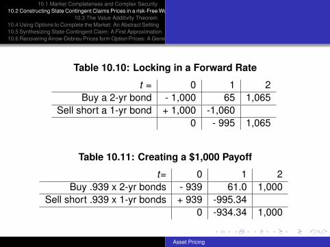
Table 10.10: Locking in a Forward Rate

t = 0 1 2Buy a 2-yr bond - 1,000 65 1,065

Sell short a 1-yr bond + 1,000 -1,0600 - 995 1,065

Table 10.11: Creating a $1,000 Payoff

t= 0 1 2Buy .939 x 2-yr bonds - 939 61.0 1,000

Sell short .939 x 1-yr bonds + 939 -995.340 -934.34 1,000

Asset Pricing



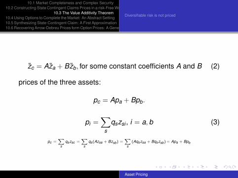
Diversifiable risk is not priced

zc = Aza + Bzb, for some constant coefficients A and B (2)

prices of the three assets:

pc = Apa + Bpb.

pi =∑

s

qszsi , i = a, b (3)

pc =X

sqszsc =

Xs

qs(Azsa + Bzsb) =X

s(Aqszsa + Bqszsb) = Apa + Bpb

Asset Pricing



Diversifiable risk is not priced

Suppose a and b are negatively correlated.c is less risky, yet pc must be «in line» with pa and Pb

Suppose a and b are perfectly negatively correlated. Canbe combined to form d, risk freepd must be such that holding d earns the riskless rateHow can the risk of a and b be remunerated

Asset Pricing



Proposition 10.3 A necessary as well as sufficient condition forthe creation of a complete set of A-D securities isthat there exists a single portfolio with the propertythat options can be written on it and such that itspayoff pattern distinguishes among all states ofnature.

Proposition 10.4 If it is possible to create, using options, acomplete set of traded securities, simple put andcall options written on the underlying assets aresufficient to accomplish this goal

Asset Pricing



It is assumed that ST discriminates across all states ofnature so that Proposition 8.1 applies; without loss ofgenerality, we may assume that ST takes the following setof values:

S1 < S2 < ... < Sθ < ... < SN ,

where Sθ is the price of this complex security if state θ isrealized at date T. Assume also that call options are written onthis asset with all possible exercised prices, and that theseoptions are traded. Let us also assume that Sθ = Sθ−1 + δ forevery state θ.

Asset Pricing



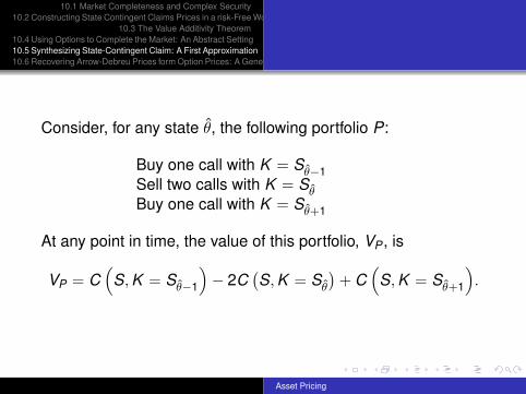
Consider, for any state θ, the following portfolio P:

Buy one call with K = Sθ−1Sell two calls with K = SθBuy one call with K = Sθ+1

At any point in time, the value of this portfolio, VP , is

VP = C(

S, K = Sθ−1

)− 2C

(S, K = Sθ

)+ C

(S, K = Sθ+1

).

Asset Pricing



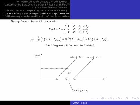
The payoff from such a portfolio thus equals:

Payoff to P =

8<:0 if ST < S

θδ if ST = S

θ0 if ST > S

θ

qθ

=1

δ

hC

“S, K = S

θ−1

”+ C

“S, K = S

θ+1

”− 2C

“S, K = S

θ

”i.

Payoff Diagram for All Options in the Portfolio P

Payoff

d

−2CT (ST, K = Sq)

ST

CT (ST, K = Sq _1)

Sq _1

CT (ST , K = Sq +1)

Sq Sq+1

d

Asset Pricing



A Generalization

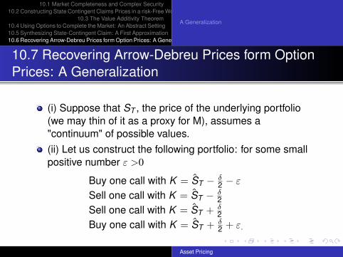
10.7 Recovering Arrow-Debreu Prices form OptionPrices: A Generalization

(i) Suppose that ST , the price of the underlying portfolio(we may thin of it as a proxy for M), assumes a"continuum" of possible values.(ii) Let us construct the following portfolio: for some smallpositive number ε >0

Buy one call with K = ST − δ2 − ε

Sell one call with K = ST − δ2

Sell one call with K = ST + δ2

Buy one call with K = ST + δ2 + ε.

Asset Pricing



A Generalization

Payoff Diagram: Portfolio of Options

ˆ

Payoff

e

CT (ST, K = ST –2)

ST

CT (ST , K = ST – 2 – e )

ST

Value of the portfolio at expiration

CT (ST, K = ST +2)

ST –2– e ST –

2ST +

2ST +

2+ e

ˆCT (ST, K = ST +

2+ e) ˆ

ˆ ˆ

d–

d–

d–

d–

d–

d–

d–

d– ˆ ˆ ˆ

ˆ ˆ

Asset Pricing



A Generalization

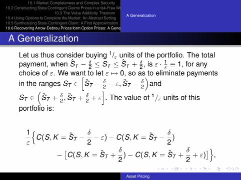
A Generalization

Let us thus consider buying 1/ε units of the portfolio. The totalpayment, when ST − δ

2 ≤ ST ≤ ST + δ2 , is ε · 1

ε ≡ 1, for anychoice of ε. We want to let ε 7→ 0, so as to eliminate paymentsin the ranges ST ∈

[ST − δ

2 − ε, ST − δ2

)and

ST ∈(

ST + δ2 , ST + δ

2 + ε]. The value of 1/ε units of this

portfolio is:

1ε

{C(S, K = ST −

δ

2− ε)− C(S, K = ST −

δ

2)

−[C(S, K = ST +

δ

2)− C(S, K = ST +

δ

2+ ε)

]},

Asset Pricing



A Generalization

limε7→0

1

ε

nC(S, K = ST −

δ

2− ε)− C(S, K = ST −

δ

2)

−ˆC(S, K = ST +

δ

2)− C(S, K = ST +

δ

2+ ε)

˜o

= − limε7→0

8>>>>><>>>>>:C

“S, K = ST − δ

2 − ε”− C

“S, K = ST − δ

2

”−ε| {z }≤0

9>>>>>=>>>>>;

+ limε7→0

8>>>>><>>>>>:C

“S, K = ST + δ

2 + ε”− C

“S, K = ST + δ

2

”ε| {z }≤0

9>>>>>=>>>>>;= C2

„S, K = ST +

δ

2

«− C2

„S, K = ST −

δ

2

«.

Asset Pricing



A Generalization

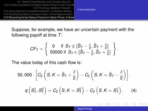
Suppose, for example, we have an uncertain payment with thefollowing payoff at time T :

CFT =

{0 if ST /∈ [ST − δ

2 , ST + δ2 ]

50000 if ST ∈ [ST − δ2 , ST + δ

2 ]

}.

The value today of this cash flow is:

50, 000 ·[C2

(S, K = ST +

δ

2

)− C2

(S, K = ST −

δ

2

)].

q(

S1T , S2

T

)= C2

(S, K = S2

T

)− C2

(S, K = S1

T

). (4)

Asset Pricing



A Generalization

Payoff Diagram for the Limiting Portfolio

Payoff

STSTST

_ _2 ST

+ _2

1

d d

Asset Pricing



A Generalization

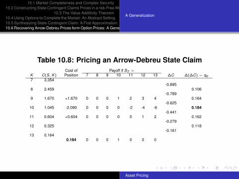
Table 10.8: Pricing an Arrow-Debreu State ClaimCost of Payoff if ST =

K C(S, K ) Position 7 8 9 10 11 12 13 ∆C ∆(∆C) = qθ7 3.354

-0.8958 2.459 0.106

-0.7899 1.670 +1.670 0 0 0 1 2 3 4 0.164

-0.62510 1.045 -2.090 0 0 0 0 -2 -4 -6 0.184

-0.44111 0.604 +0.604 0 0 0 0 0 1 2 0.162

-0.27912 0.325 0.118

-0.16113 0.164

0.184 0 0 0 1 0 0 0

Asset Pricing

Date post:	29-Aug-2018
Category:	Documents
Upload:	duongdieu
View:	219 times
Download:	0 times

Asset Pricing - Chapter X. Arrow-Debreu pricing II: The ... for... · value (ii) 55 8 % bond priced...

Documents