Assignment week 38

Exponential smoothing of monthly observations of the General Index of the Stockholm Stock Exchange.

A. Graphical illustration of data

First, construct a graph of the original series of monthly values.

610549488427366305244183122611

4000

3000

2000

1000

0

Index

Index

Time Series Plot of Index

Stock_Exchange.txt

Then construct a graph of the percentage change from month to month.

610549488427366305244183122611

30

20

10

0

-10

-20

Index

Change

Time Series Plot of Change

Which smoothing techniques (single, double, Holt-Winters) can be used on the original series, which can be used on the series of percentage change.

Original series: Double (Holt’s) (or Holt-Winters’ (Winters’) method)

Series of percentage change: Single (or Winters’ without trend)

B. Exponential smoothing with predefined smoothing parameters

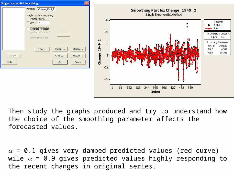
Perform single exponential smoothing on the time series of percentage change (of the General Indices). Set the smoothing parameter, , first to 0.9 and then to 0.1.

Variable Change is not in the list, due to the initial missing value Copy the non-missing values to a new column.

549488427366305244183122611

30

20

10

0

-10

-20

Index

Change_1949_2

Alpha 0.1Smoothing Constant

MAPE 160.999MAD 3.514MSD 23.053

Accuracy Measures

ActualFits

Variable

Smoothing Plot for Change_1949_2Single Exponential Method

549488427366305244183122611

30

20

10

0

-10

-20

Index

Change_1949_2

Alpha 0.9Smoothing Constant

MAPE 240.685MAD 4.382MSD 35.101

Accuracy Measures

ActualFits

Variable

Smoothing Plot for Change_1949_2Single Exponential Method

Then study the graphs produced and try to understand how the choice of the smoothing parameter affects the forecasted values.

= 0.1 gives very damped predicted values (red curve) wile = 0.9 gives predicted values highly responding to the recent changes in original series.

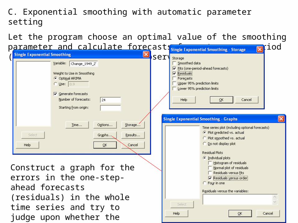
C. Exponential smoothing with automatic parameter setting

Let the program choose an optimal value of the smoothing parameter and calculate forecasts for a two-year period (24 months) after the last observed time-point.

Construct a graph for the errors in the one-step-ahead forecasts (residuals) in the whole time series and try to judge upon whether the forecasting methods uses earlier observations in the series in an efficient way.

630567504441378315252189126631

30

20

10

0

-10

-20

Index

Change_1949_2

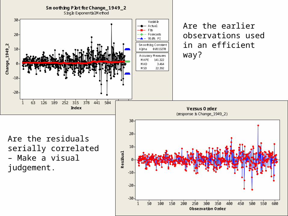
Alpha 0.0113270Smoothing Constant

MAPE 141.322MAD 3.464MSD 22.392

Accuracy Measures

ActualFitsForecasts95.0% PI

Variable

Smoothing Plot for Change_1949_2Single Exponential Method

600550500450400350300250200150100501

30

20

10

0

-10

-20

-30

Observation Order

Resi

dual

Versus Order(response is Change_1949_2)

Are the residuals serially correlated – Make a visual judgement.

Are the earlier observations used in an efficient way?

Use also the autocorrelation function on the residual. (MINITAB-Time Series- Autocorrelation).

65605550454035302520151051

1.0

0.8

0.6

0.4

0.2

0.0

-0.2

-0.4

-0.6

-0.8

-1.0

Lag

Auto

corr

ela

tion

Autocorrelation Function for RESI1(with 5% significance limits for the autocorrelations)

What do you see in the plot you get?

First spike is significantly different from zero, so is also some spikes for larger lags.

Residuals seem to be serially correlated.

Exponential smoothing of time series with seasonal variation

A. Forecasting the employment in USA

Perform an exponential smoothing of the time series of monthly employments figures in USA and calculate forecasts for a two-year period (24 month) after the last observed time-point.

Labourforce.txt

600540480420360300240180120601

68

66

64

62

60

58

56

Index

Valu

e

Time Series Plot of Value

Time series possesses trend and seasonal variation Use Winters’ method

Seasonal variation do not seem to change with level Use additive case

620558496434372310248186124621

70

68

66

64

62

60

58

56

Index

Valu

e

Alpha (level) 0.2Gamma (trend) 0.2Delta (seasonal) 0.2

Smoothing Constants

MAPE 0.370202MAD 0.226105MSD 0.086981

Accuracy Measures

ActualFitsForecasts95.0% PI

Variable

Winters' Method Plot for ValueAdditive Method

Then use a suitable model for time series decomposition to make forecasts for the same period (additive or multiplicative).

620558496434372310248186124621

70.0

67.5

65.0

62.5

60.0

57.5

55.0

Index

Valu

e

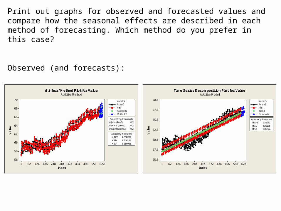
MAPE 1.41981MAD 0.86505MSD 1.05524

Accuracy Measures

ActualFitsTrendForecasts

Variable

Time Series Decomposition Plot for ValueAdditive Model

Print out graphs for observed and forecasted values and compare how the seasonal effects are described in each method of forecasting. Which method do you prefer in this case?

Observed (and forecasts):

620558496434372310248186124621

70

68

66

64

62

60

58

56

Index

Valu

e

Alpha (level) 0.2Gamma (trend) 0.2Delta (seasonal) 0.2

Smoothing Constants

MAPE 0.370202MAD 0.226105MSD 0.086981

Accuracy Measures

ActualFitsForecasts95.0% PI

Variable

Winters' Method Plot for ValueAdditive Method

620558496434372310248186124621

70.0

67.5

65.0

62.5

60.0

57.5

55.0

Index

Valu

e

MAPE 1.41981MAD 0.86505MSD 1.05524

Accuracy Measures

ActualFitsTrendForecasts

Variable

Time Series Decomposition Plot for ValueAdditive Model

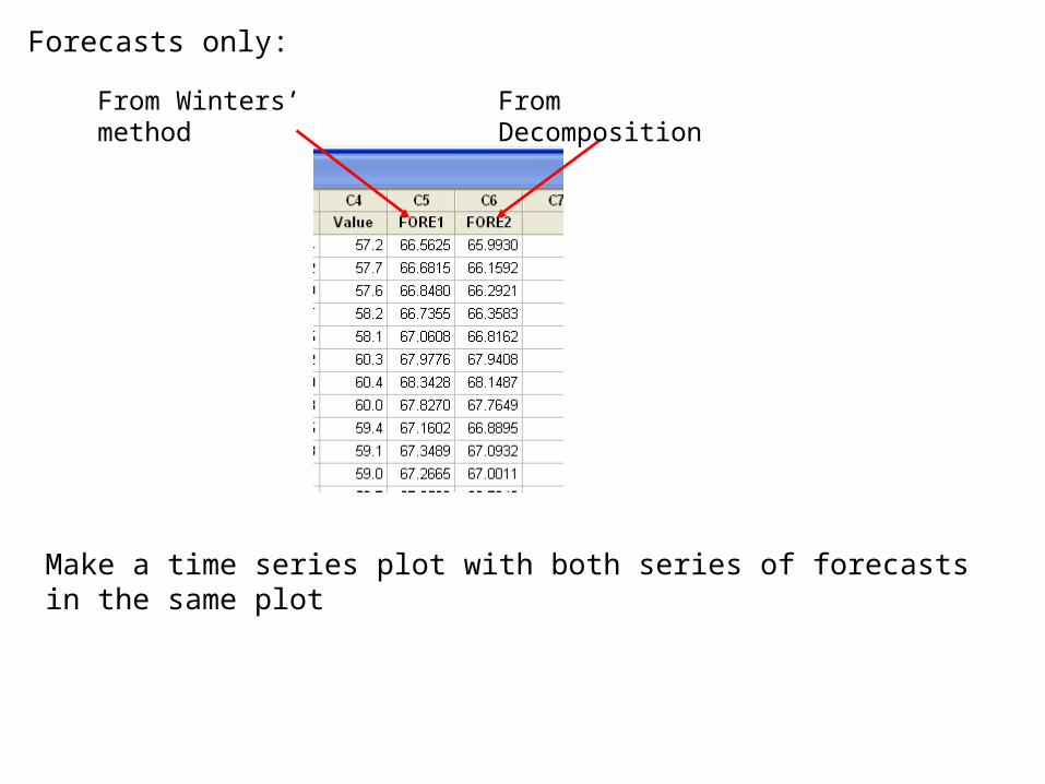
Forecasts only:

From Winters’ method From Decomposition

Make a time series plot with both series of forecasts in the same plot

24222018161412108642

68.5

68.0

67.5

67.0

66.5

66.0

Index

Data

FORE1FORE2

Variable

Time Series Plot of FORE1, FORE2

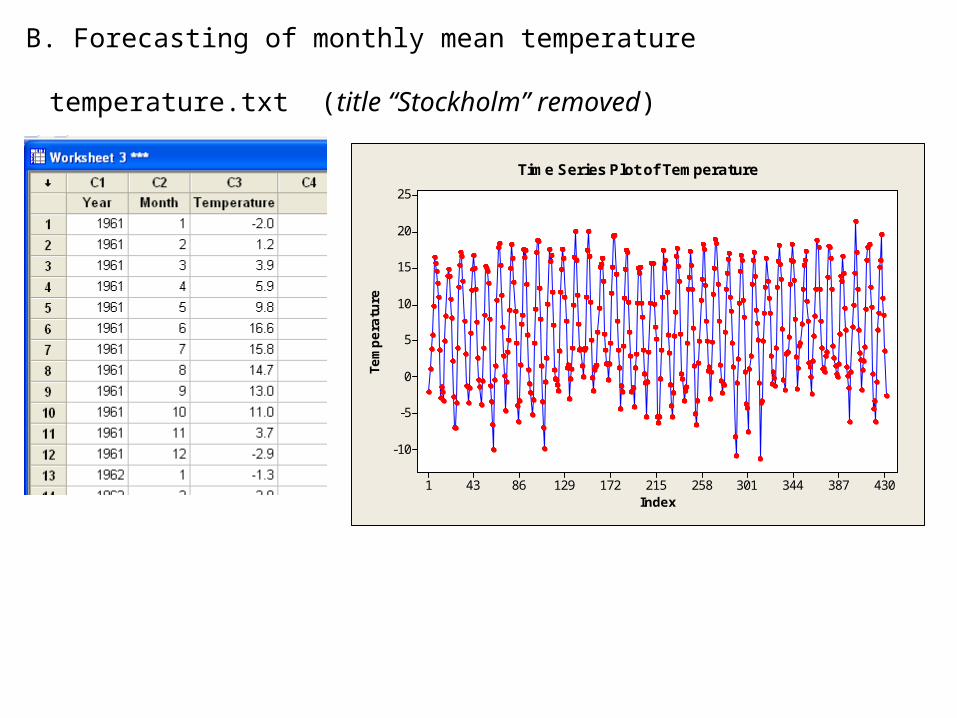
B. Forecasting of monthly mean temperature

temperature.txt (title “Stockholm” removed)

43038734430125821517212986431

25

20

15

10

5

0

-5

-10

Index

Tem

pera

ture

Time Series Plot of Temperature

Use exponential smoothing to make forecasts of monthly mean temperatures in Stockholm. Try single, double (Holt’s method) and Winters’ method.

Study the residuals (the errors in one-step-ahead forecasts) and the forecasts for 24 months after the last observed time-point. Are the one-month-ahead and one-year-ahead forecasts realistic?

Single exponential smoothing:

41436832227623018413892461

20

10

0

-10

-20

Index

Tem

pera

ture Alpha 1.39083

Smoothing Constant

MAPE 144.034MAD 3.198MSD 15.636

Accuracy Measures

ActualFitsForecasts95.0% PI

Variable

Smoothing Plot for TemperatureSingle Exponential Method

400350300250200150100501

10

5

0

-5

-10

Observation Order

Resi

dual

Versus Order(response is Temperature)

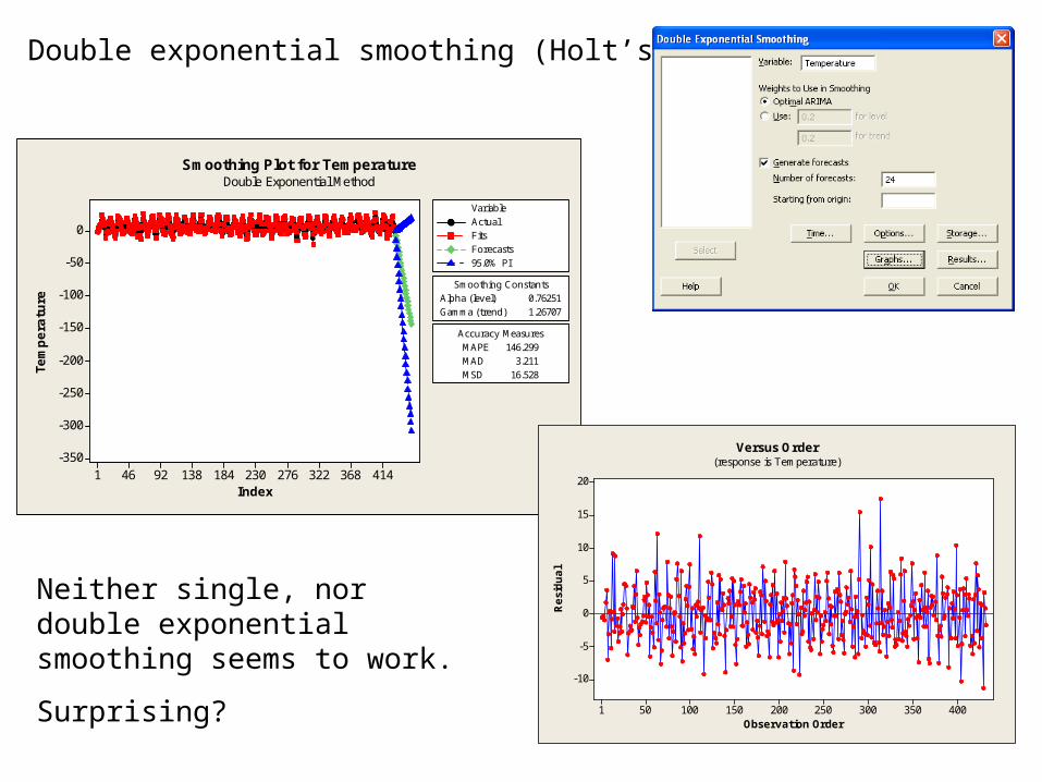
Double exponential smoothing (Holt’s method):

41436832227623018413892461

0

-50

-100

-150

-200

-250

-300

-350

Index

Tem

pera

ture Alpha (level) 0.76251

Gamma (trend) 1.26707

Smoothing Constants

MAPE 146.299MAD 3.211MSD 16.528

Accuracy Measures

ActualFitsForecasts95.0% PI

Variable

Smoothing Plot for TemperatureDouble Exponential Method

400350300250200150100501

20

15

10

5

0

-5

-10

Observation Order

Resi

dual

Versus Order(response is Temperature)

Neither single, nor double exponential smoothing seems to work.

Surprising?

Winters’ method:

Note that we do not have any particularly pronounced trend in data and shifts in level are (if existing) very modest.

43038734430125821517212986431

25

20

15

10

5

0

-5

-10

Index

Tem

pera

ture

Time Series Plot of Temperature

Try low values of smoothing parameters for level and trend

41436832227623018413892461

30

20

10

0

-10

Index

Tem

pera

ture Alpha (level) 0.05

Gamma (trend) 0.01Delta (seasonal) 0.20

Smoothing Constants

MAPE 108.557MAD 2.490MSD 10.021

Accuracy Measures

ActualFitsForecasts95.0% PI

Variable

Winters' Method Plot for TemperatureAdditive Method

400350300250200150100501

5

0

-5

-10

Observation Order

Resi

dual

Versus Order(response is Temperature)

Residuals become positively correlated

Forecasts much better here

Compare with an analysis with default values on smoothing parameters:

41436832227623018413892461

30

20

10

0

-10

Index

Tem

pera

ture Alpha (level) 0.2

Gamma (trend) 0.2Delta (seasonal) 0.2

Smoothing Constants

MAPE 95.4625MAD 1.8182MSD 5.2691

Accuracy Measures

ActualFitsForecasts95.0% PI

Variable

Winters' Method Plot for TemperatureAdditive Method

400350300250200150100501

10

5

0

-5

-10

Observation Order

Resi

dual

Versus Order(response is Temperature)

Residuals are much better.

Forecasts seem to contain an “artificially” induced trend.

We have to keep on trying.

Is there a better way for making forecasts than applying exponential smoothing on the original series?