56
Assimilating satellite cloud information with an Ensemble Kalman Filter at the convective scale Annika Schomburg, Christoph Schraff EUMETSAT fellow day, 17 March 2014, Darmstadt
| Date post: | 20-Jan-2016 |
| Category: |
Documents |
| Upload: | jonas-perry |
| View: | 233 times |
| Download: | 3 times |

Assimilating satellite cloud information with an Ensemble
Kalman Filter at the convective scale
Annika Schomburg, Christoph Schraff
EUMETSAT fellow day, 17 March 2014, Darmstadt
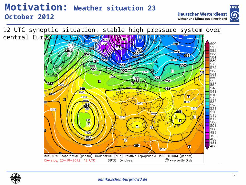
Motivation: Weather situation 23 October 2012
2
12 UTC synoptic situation: stable high pressure system over central Europe

Motivation: Weather situation 23 October 2012
3
12 UTC synoptic situation: low stratus clouds over Germany
Satellite cloud type classification

Motivation: Verification for 23 October 2012
4
12 hour forecast from 0:00 UTC
Low cloud cover: COSMO-DE versus satellite
Total cloud cover: COSMO-DE versus synop
T2m: COSMO-DE minus synop
Green: hits; black: missesred: false alarms, blue: no obs
Courtesy of K. Stephan

Motivation
Main motivation: improve cloud cover simulation of low stratus clouds in stable wintertime high-pressure systems
•May also be useful for frontal system or convective situations
• If convective clouds are captured better while developing, convective precipitation may be improved
5

• Introduction
• The COSMO model
• The ensemble Kalman filter
Outline
6
• Cloud data
• Assimilation approach• Assimilated variables and model
equivalents
• Results• Single observation experiments• Cycling experiment• Forecast
• Conclusion and outlook• Future application
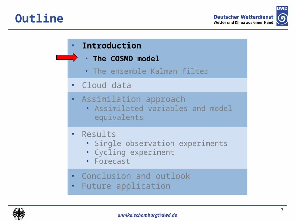
• Introduction
• The COSMO model
• The ensemble Kalman filter
Outline
7
• Cloud data
• Assimilation approach• Assimilated variables and model
equivalents
• Results• Single observation experiments• Cycling experiment• Forecast
• Conclusion and outlook• Future application
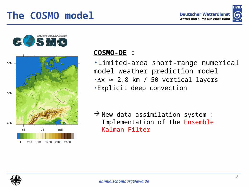
The COSMO model
8
COSMO-DE :
•Limited-area short-range numerical model weather prediction model•x 2.8 km / 50 vertical layers •Explicit deep convection
New data assimilation system : Implementation of the Ensemble Kalman Filter

• Introduction
• The COSMO model
• The ensemble Kalman filter
Outline
9
• Cloud data
• Assimilation approach• Assimilated variables and model
equivalents
• Results• Single observation experiments• Cycling experiment• Forecast
• Conclusion and outlook• Future application

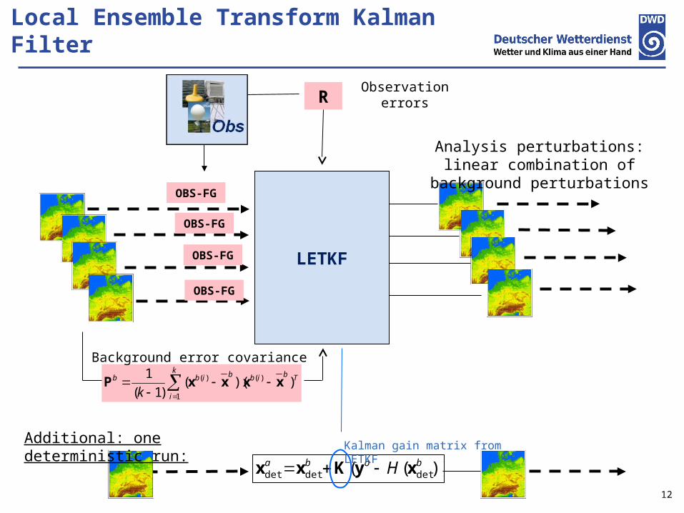
Local Ensemble Transform Kalman Filter
LETKF
Analysis perturbations: linear combination of background
perturbations
First guess ensemble members are weighted according to their departure from the observations.
OBS-FG
OBS-FG
OBS-FG
OBS-FG
R
Tbibk
i
bibb
k))((
)1(
1 )(
1
)( xxxxP
Background error covariance
Observation errors

Local Ensemble Transform Kalman Filter
LETKF
Analysis perturbations: linear combination of background
perturbationsOBS-FG
OBS-FG
OBS-FG
OBS-FG
R
Tbibk
i
bibb
k))((
)1(
1 )(
1
)( xxxxP
Observation errors
11
• Local: the linear combination is fitted in a local region
- observation have a spatially limited influence region
• Transform: most computations are carried out in ensemble space computationally efficient
Implementation after Hunt et al., 2007
Background error covariance
Local Ensemble Transform Kalman Filter
LETKF
Analysis perturbations: linear combination of background
perturbationsOBS-FG
OBS-FG
OBS-FG
OBS-FG
R
Tbibk
i
bibb
k))((
)1(
1 )(
1
)( xxxxP
Background error covariance
Observation errors
Additional: one deterministic run:
))(( detdetdetboba H xyKxx
Kalman gain matrix from LETKF
12

• Introduction
• The COSMO model
• The ensemble Kalman filter
Outline
13
• Cloud data
• Assimilation approach• Assimilated variables and model
equivalents
• Results• Single observation experiments• Cycling experiment• Forecast
• Conclusion and outlook• Future application

Which observations?
For shortrange limited-area models: geostationary satellite data: Meteosat-SEVIRI (Δx ~ 5km over central Europe, Δt=15 min)
Here: Assimilation of NWC-SAF cloud top height
Source: EUMETSAT
Height [km]
Cloud top height
1 2 3 4 5 6 7 8 9 10 11 12 13
14
Retrieval algorithm needs temperature and humidity profile information from a NWP model cloud top height might be at wrong height if temperature-profile in NWP model is not simulated correctly! use also radiosonde information where available
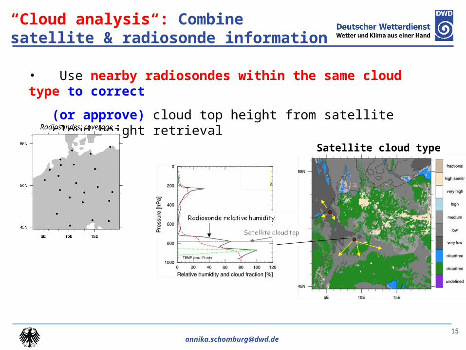
“Cloud analysis“: Combine satellite & radiosonde information
• Use nearby radiosondes within the same cloud type to correct
(or approve) cloud top height from satellite cloud height retrieval
Radiosondes: coverage
Satellite cloud type

Combine satellite & radiosonde information: data availability flag
• Use temporal and spatial distance of radiosonde for weighting:
• Also use data availability flag for observation error specification:
1.0
0.8
0.6
0.4
0.2
rssatcorr cthcthcth )1(
γ
rssato eee )1(

Combine satellite & radiosonde information
Satellite cloud product Cloud analysis
Cloud top height
Obs-error [m]

• Introduction
• The COSMO model
• The ensemble Kalman filter
Outline
18
• Cloud data
• Assimilation approach• Assimilated variables and model
equivalents
• Results• Single observation experiments• Cycling experiment• Forecast
• Conclusion and outlook• Future application
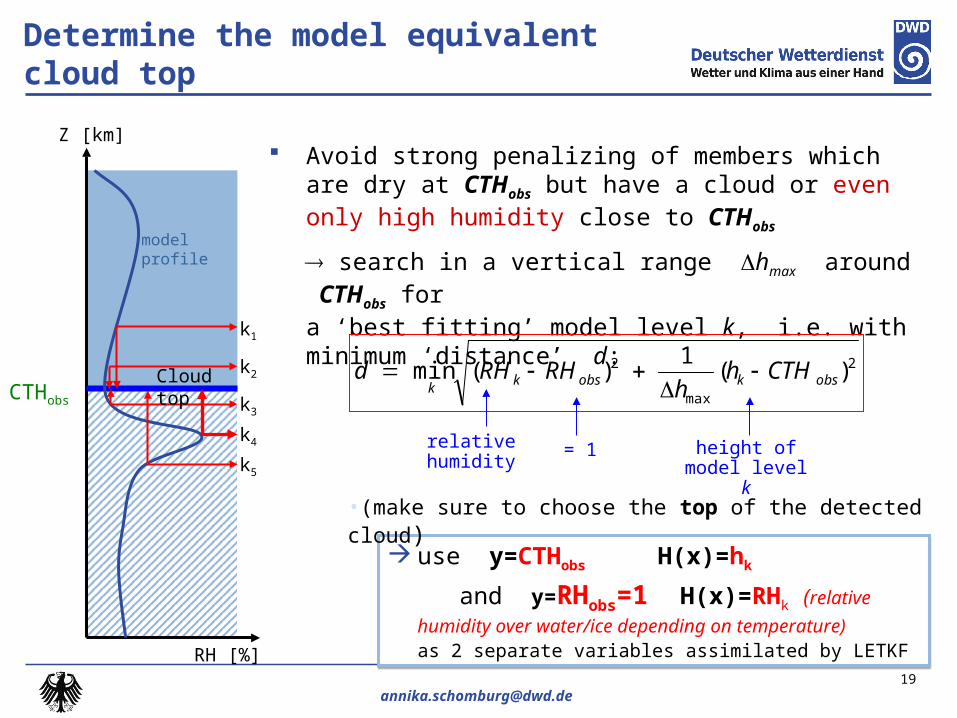
Determine the model equivalent cloud top
Avoid strong penalizing of members which are dry at CTHobs but have a cloud or even only high humidity close to CTHobs
search in a vertical range hmax around CTHobs fora ‘best fitting’ model level k, i.e. with minimum ‘distance’ d:
2
max
2 )(1
)(min obskobskk
CTHhh
RHRHd
relative humidity height ofmodel level
k
= 1
use y=CTHobs H(x)=hk
and y=RHobs=1 H(x)=RHk (relative humidity over
water/ice depending on temperature)as 2 separate variables assimilated by LETKF
use y=CTHobs H(x)=hk
and y=RHobs=1 H(x)=RHk (relative humidity over
water/ice depending on temperature)as 2 separate variables assimilated by LETKF
19
Z [km]
RH [%]
CTHobs
k1
k2
k3
k4
k5
Cloud top
model profile
•(make sure to choose the top of the detected cloud)
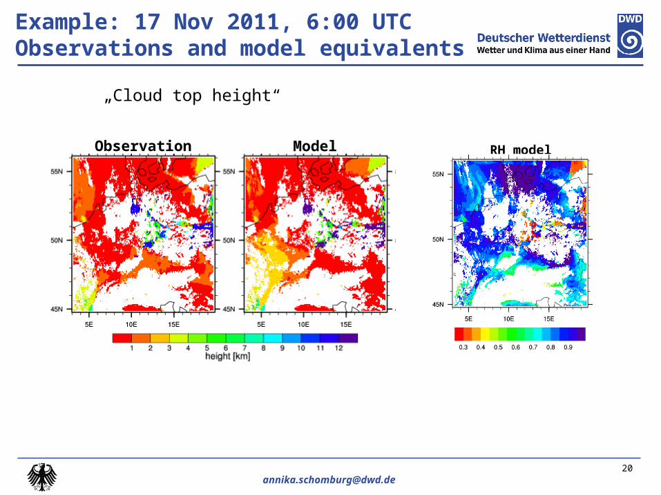
Example: 17 Nov 2011, 6:00 UTCObservations and model equivalents
RH model level kObservation Model
„Cloud top height“

3
6
9
12
Z [km]
„no high cloud“
„no mid-level cloud“
„no low cloud“
CLC
• assimilate cloud fraction CLC = 0 separately
for high, medium, low clouds
• model equivalent:
maximum CLC within vertical range
What information can we assimilate for pixels which are observed to be cloudfree?
Determine model equivalent: cloudfree pixels
21

COSMO cloud cover where observations “cloudfree”
Example: 17 Nov 2011, 6:00 UTC
High clouds (oktas)Mid-level clouds (oktas)Low clouds (oktas)
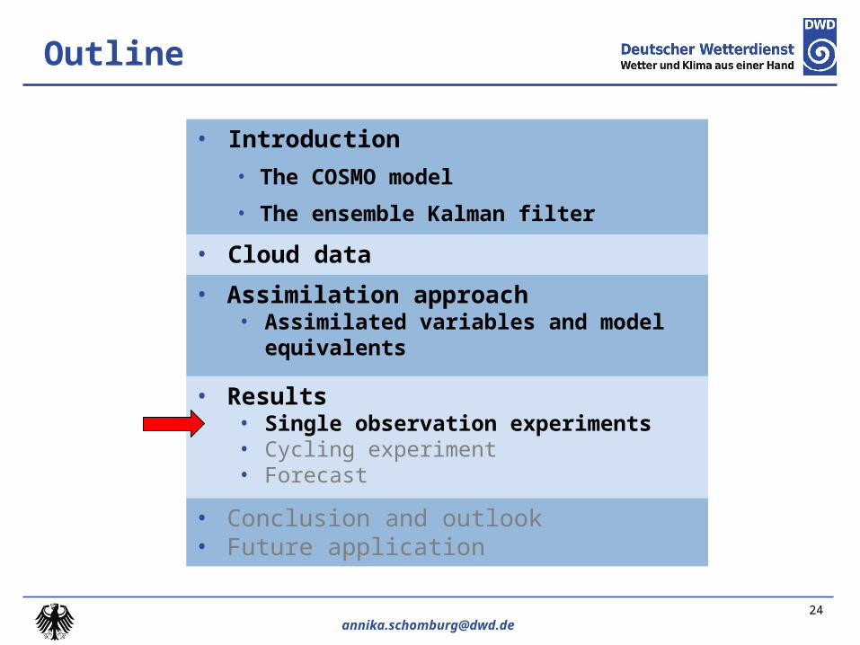
• Introduction
• The COSMO model
• The ensemble Kalman filter
Outline
24
• Cloud data
• Assimilation approach• Assimilated variables and model
equivalents
• Results• Single observation experiments• Cycling experiment• Forecast
• Conclusion and outlook• Future application

„Single observation“ experiment
• Analysis for 17 November 2011, 6:00 UTC (no cycling)
• Each column is affected by only one satellite observation
• Objective:– Understand in detail what the filter does with such special
observation types– Does it work at all?– Detailed evaluation of effect on atmospheric profiles– Sensitivity to settings

relative humiditycloud covercloud water
cloud iceobserved cloud top
3 lines in one colour indicate ensemble mean and mean +/- spread
• 1 analysis step, 17 Nov. 2011, 6 UTC (wintertime low stratus)
vertical profiles
Single-observation experiments: missed cloud event
26

observed cloud top
observation location
specific water content [g/kg] relative humidity [%]
Cross section of analysis increments for ensemble mean
Single-observation experiments: missed cloud event
27

Deterministic run
Humidity at cloud layer is increased in deterministic run
Relative humidity
Cloud cover
Cloud water
Cloud ice
Observed cloud top
First guess Analysis
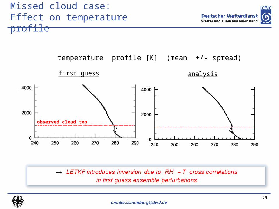
Missed cloud case:Effect on temperature profile
temperature profile [K] (mean +/- spread)
first guess analysis
observed cloud top
29
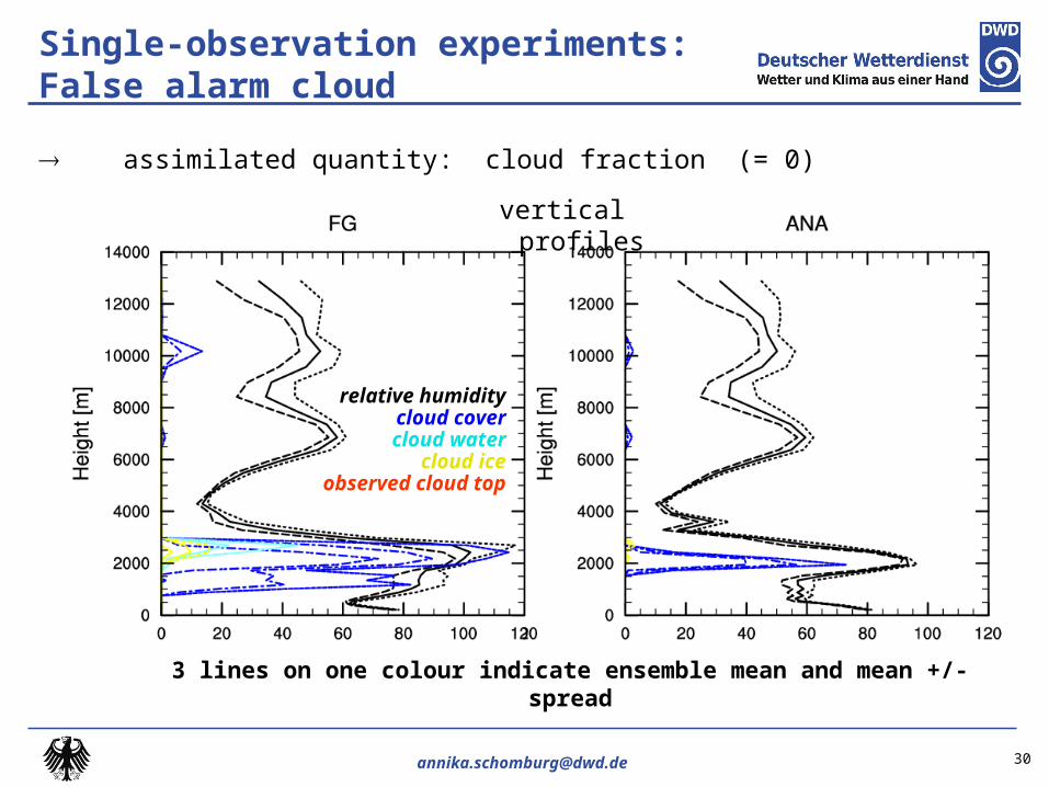
relative humiditycloud covercloud water
cloud iceobserved cloud top
3 lines on one colour indicate ensemble mean and mean +/- spread
vertical profiles
assimilated quantity: cloud fraction (= 0)
Single-observation experiments: False alarm cloud
30

• Observation cloudfree assimilated quantity: cloud fraction (= 0)
FG
ANA
low cloud cover fraction [octa] mid-level cloud cover fraction [octa]
Observation minus model histogram over ensemble members
FG
ANA
Single-observation experiments: False alarm cloud
32
• Introduction
• The COSMO model
• The ensemble Kalman filter
Outline
33
• Cloud data
• Assimilation approach• Assimilated variables and model
equivalents
• Results• Single observation experiments• Cycling experiment• Forecast
• Conclusion and outlook• Future application
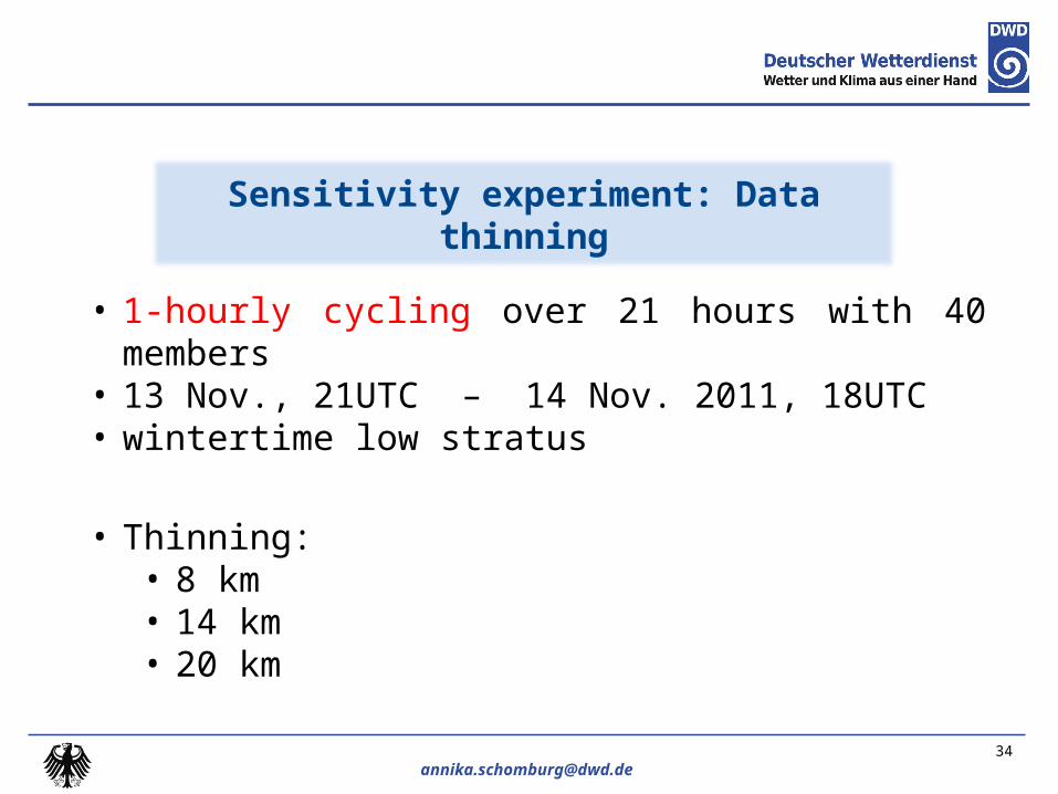
• 1-hourly cycling over 21 hours with 40 members• 13 Nov., 21UTC – 14 Nov. 2011, 18UTC• wintertime low stratus
• Thinning: • 8 km• 14 km• 20 km
Sensitivity experiment: Data thinning
34

Sensitivity experiment: Data density
Comparing experiments with different data density:
• 8 km
• 14 km
• 20km
35
For cloudy pixels best results are obtained for a 14 km thinning distance, for For cloudy pixels best results are obtained for a 14 km thinning distance, for cloud-free observations no clear conclusioncloud-free observations no clear conclusion
RMSE and bias averaged over all cloudy observations
RMSE
Bias (OBS-FG)
Mean squared error for low/medium/high cloud cover averaged over all
observed cloud free pixels
Low cloudsMid-level cloudsHigh cloudsSolid: 8kmDashed: 14kmDotted: 20km
RH at observed cloud top Cloud cover
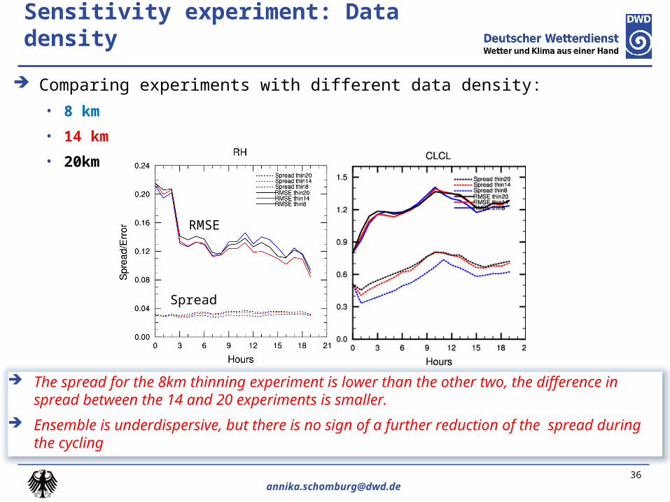
The spread for the 8km thinning experiment is lower than the other two, the difference in spread between the 14 and 20 experiments is smaller.
Ensemble is underdispersive, but there is no sign of a further reduction of the spread during the cycling
36
Comparing experiments with different data density:
• 8 km
• 14 km
• 20km
Sensitivity experiment: Data density
RMSE
Spread
• 1-hourly cycling over 21 hours with 40 members• 13 Nov., 21UTC – 14 Nov. 2011, 18UTC• Wintertime low stratus
• Thinning: 14 km
Comparison cycling experiment: only conventional
vs conventional + cloud data
37

Time series of first guess errors, averaged over cloudy obs locations
assimilation of conventional obs only assimilation of conventional + cloud obs
RMSE
Bias (OBS-FG)
38
Comparison “only conventional“ versus “conventional + cloud obs"
RH (relative humidity) at observed cloud top
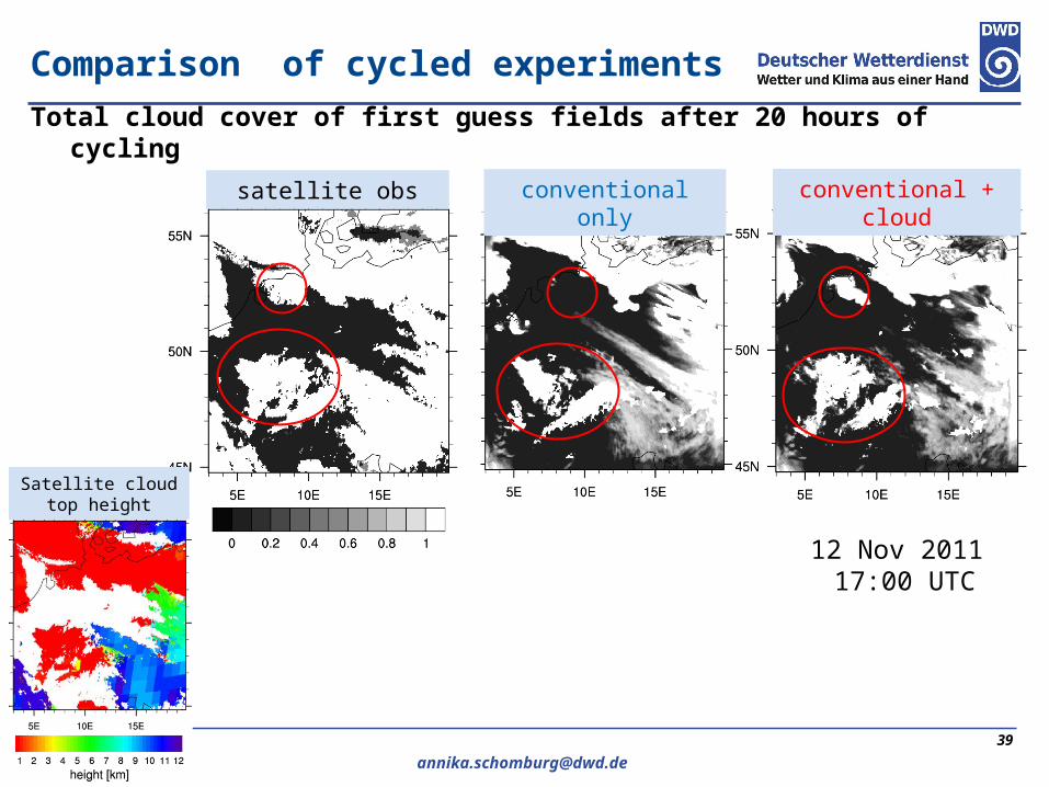
conventional only conventional + cloud
Total cloud cover of first guess fields after 20 hours of cycling
Satellite cloud top height
Comparison of cycled experiments
satellite obs
12 Nov 2011 17:00 UTC

Time series of first guess errors, averaged over cloud-free obs locations(errors are due to false alarm clouds)
mean square error of cloud fraction [octa]
False alarm clouds False alarm clouds reduced through cloud reduced through cloud data assimilationdata assimilation
Cycled assimilation of dense observations
40
low clouds
High clouds
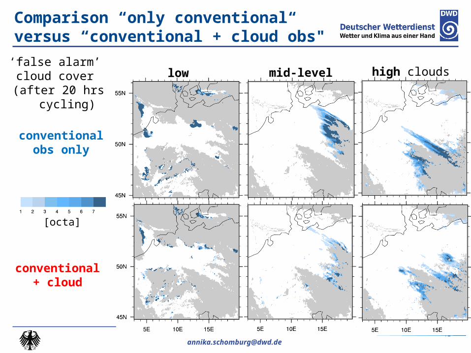
low clouds mid-level clouds high clouds‘false alarm’ cloud cover
(after 20 hrs cycling)
conventional+ cloud
conventionalobs only
41
Comparison “only conventional“ versus “conventional + cloud obs"
[octa]

• Introduction
• The COSMO model
• The ensemble Kalman filter
Outline
42
• Cloud data
• Assimilation approach• Assimilated variables and model
equivalents
• Results• Single observation experiments• Cycling experiment• Forecast
• Conclusion and outlook• Future application

• 24h deterministic forecast based on analysis of two experiments (after 12 hours of cycling)
• 14 Nov., 9UTC – 15 Nov. 2011, 9UTC• Wintertime low stratus
Comparison forecast experiment: only conventional
vs conventional + cloud data
43

The forecast of cloud characteristics can be improved through the assimilation of the cloud information
44
Comparison of free forecast: time series of errors
Conventional + cloud dataOnly conventional data
RMSE
Bias (Obs-Model)
Low cloudsMid-level cloudsHigh clouds
Mean squared error averaged over all cloud-free observations
RH (relative humidity) at observed cloud top averaged over all cloudy
observations
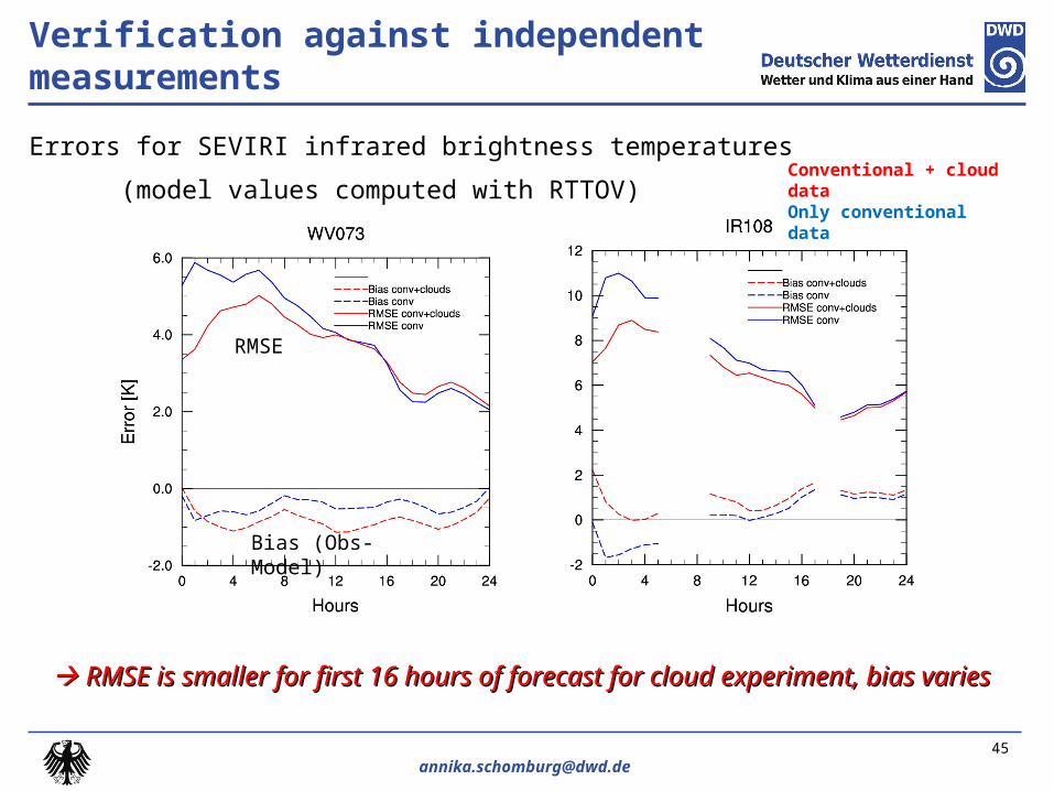
Verification against independent measurements
Errors for SEVIRI infrared brightness temperatures
(model values computed with RTTOV)
45
RMSE is smaller for first 16 hours of forecast for cloud experiment, bias variesRMSE is smaller for first 16 hours of forecast for cloud experiment, bias varies
RMSE
Bias (Obs-Model)
Conventional + cloud dataOnly conventional data

CONV+CLOUD experiment
Only CONV experiment
Also the high clouds are simulated better in the cloud experiment Also the high clouds are simulated better in the cloud experiment 46
Verification against independent measurements: SEVIRI brightness temperature errors
Cloud top height14 Nov 2011,
18 UTC

• Introduction
• The COSMO model
• The ensemble Kalman filter
Outline
47
• Cloud data
• Assimilation approach• Assimilated variables and model
equivalents
• Results• Single observation experiments• Cycling experiment• Forecast
• Conclusion and outlook• Future application

Use of (SEVIRI-based) cloud observations in LETKF:
•Tends to introduce humidity / cloud where it should (+ temperature inversion)
•Tends to reduce ‘false-alarm’ clouds
•Despite non-Gaussian pdf’s
•Long-lasting free forecast impact for a stable wintertime high pressure system
Conclusions
48

• Evaluate impact on other variables (temperature, wind)
• Other cases (e.g. convective)
• Also work on direct SEVIRI radiance assimilation
• Revision on QJRMS article on single observation experiments, publish second article on full cycling and forecasts results
• Application in renewable energy project EWeLiNE…
Next steps
49

• Introduction
• The COSMO model
• The ensemble Kalman filter
Outline
50
• Cloud data
• Assimilation approach• Assimilated variables and model
equivalents
• Results• Single observation experiments• Cycling experiment• Forecast
• Conclusion and outlook• Future application
Renewable energy project
• Germany plans to increase the percentage of renewable energy to 35% in 2020
Increasing demands for accurate power predictions for a safe and cost-effective power system
Joint project of DWD and Fraunhofer-Institut for Wind Energy & Energy System Technology in Kassel and three transmission network operators EWeLiNE
• Objective: improve weather and power forecasts for wind and phovoltaic power and develop new prognostic products
• 4 year project, 13 researchers at DWD

Problematic weather situations for photovoltaic power prediction
Cloud cover after cold front pass
Convective situations
Low stratus / fog weather situations
Snow coverage of photovoltaic modules
52

Problematic weather situations for photovoltaic power prediction
Cloud cover after cold front pass
Convective situations
Low stratus / fog weather situations
Snow coverage of photovoltaic modules
53

Problematic weather situations for photovoltaic power prediction
Cloud cover after cold front pass
Convective situations
Low stratus / fog weather situations
Snow coverage of photovoltaic modules
54

Hochrechnung
Example: problematic weather situation: low stratus clouds
Error Day-Ahead: 4800 MW
Low stratus clouds not predicted
Low stratus clouds observed in reality
ProjectionDay-AheadIntra-Day
time
Power from PV modules
courtesy by TENNET
55

Thank you for your attention!Thank you for your attention!
Thanks to EUMETSAT for funding this fellowship!Thanks to EUMETSAT for funding this fellowship!


