Page 1
Int. J. Environ. Res. Public Health 2014, 11, 7376-7392; doi:10.3390/ijerph110707376
International Journal of
Environmental Research and
Public Health ISSN 1660-4601
www.mdpi.com/journal/ijerph
Article
Associations between Perceptions of Drinking Water Service
Delivery and Measured Drinking Water Quality in Rural
Alabama
Jessica C. Wedgworth 1, Joe Brown
2, Pauline Johnson
3, Julie B. Olson
1, Mark Elliott
3,
Rick Forehand 4 and Christine E. Stauber
5,*
1 Department of Biological Sciences, University of Alabama, 300 Hackberry Lane, Tuscaloosa,
AL 35487, USA; E-Mails: [email protected] (J.C.W.); [email protected] (J.B.O.) 2 School of Civil and Environmental Engineering, Georgia Institute of Technology, 311 Ferst Drive,
Atlanta, GA 30332, USA; E-Mail: [email protected] 3 Department of Civil and Environmental Engineering, University of Alabama, 245 7th Avenue,
Tuscaloosa, AL 35487, USA; E-Mails: [email protected] (P.J.); [email protected] (M.E.) 4
Barge Waggoner Sumner and Cannon Inc., 2047 West Main Street, Suite 1, Dothan, AL 36301,
USA; E-Mail: [email protected] 5 Division of Environmental Health, School of Public Health, Georgia State University,
P.O. Box 3995, Atlanta, GA 30302, USA
* Author to whom correspondence should be addressed; E-Mail: [email protected] ;
Tel.: +1-404-413-1128; Fax: +1-404-413-1140.
Received: 17 March 2014; in revised form: 3 June 2014 / Accepted: 30 June 2014 /
Published: 18 July 2014
Abstract: Although small, rural water supplies may present elevated microbial risks to
consumers in some settings, characterizing exposures through representative
point-of-consumption sampling is logistically challenging. In order to evaluate the
usefulness of consumer self-reported data in predicting measured water quality and risk
factors for contamination, we compared matched consumer interview data with
point-of-survey, household water quality and pressure data for 910 households served by
14 small water systems in rural Alabama. Participating households completed one survey
that included detailed feedback on two key areas of water service conditions: delivery
conditions (intermittent service and low water pressure) and general aesthetic
characteristics (taste, odor and color), providing five condition values. Microbial water
samples were taken at the point-of-use (from kitchen faucets) and as-delivered from the
OPEN ACCESS
Page 2
Int. J. Environ. Res. Public Health 2014, 11 7377
distribution network (from outside flame-sterilized taps, if available), where pressure was
also measured. Water samples were analyzed for free and total chlorine, pH, turbidity, and
presence of total coliforms and Escherichia coli. Of the 910 households surveyed, 35% of
participants reported experiencing low water pressure, 15% reported intermittent service,
and almost 20% reported aesthetic problems (taste, odor or color). Consumer-reported low
pressure was associated with lower gauge-measured pressure at taps. While total coliforms
(TC) were detected in 17% of outside tap samples and 12% of samples from kitchen
faucets, no reported water service conditions or aesthetic characteristics were associated
with presence of TC. We conclude that consumer-reported data were of limited utility in
predicting potential microbial risks associated with small water supplies in this setting,
although consumer feedback on low pressure—a risk factor for contamination—may be
relatively reliable and therefore useful in future monitoring efforts.
Keywords: small water supply; rural; water quality; perceived service; drinking water
quality; infrastructure; environmental health
1. Introduction
Small, rural, and economically disadvantaged communities in the USA face a variety of challenges,
including aging infrastructure. Water supply infrastructure, operation, and maintenance may be
sub-optimal in such settings, where revenues for critical investments and ongoing maintenance may be
lacking due to such factors as low population densities, geographically large service areas, and
limitations on revenues due to an inadequate economic base or rate structures that do not account for
the full economic costs of the systems [1]. Although over 80% of the public water distribution systems
in the USA are classified as ―small‖ (i.e., serving fewer than 3300 persons), relatively little research
characterizing the environmental health risks associated with small water systems in resource-limited
settings of the USA has been conducted. Small water systems serve sizeable percentages of the
populations of some states (e.g., 25% in Alabama, 58% in Mississippi) and an estimated 58.5 million
people in the southeastern USA [2], but they serve a small percentage of the overall US population
(~8%). However, small systems have been linked to a disproportionate number of disease outbreaks
and have more reported violations under the Safe Drinking Water Act [3,4]. It has also been reported
that small systems may experience more frequent interruptions in service, therefore increasing the risk
for contamination [5]. From 1997-2012, small water systems in Alabama reported 129 health-based
violations per 100,000 people, which is more than 40 times greater than the total number of violations
per 100,000 people reported for large water systems during the same reporting period [6]. Thus, in
terms of microbial risks, small water systems deserve increased and sustained attention [7].
Despite this need, monitoring microbial quality in small water systems is a challenge. For smaller
systems, monitoring resources are modest; therefore their allocation is limited to meeting the
regulatory requirements (typically, three samples per month for total coliforms under routine
monitoring for systems serving ≤ 3300 people). Gathering reliable, representative data on water quality
in rural areas can be logistically complex, costly, and time-consuming, though such data may be useful
Page 3
Int. J. Environ. Res. Public Health 2014, 11 7378
in identifying priorities for water quality risk management. These data are also required for studies of
environmental health that attempt to quantify the association between microbial water quality and
health outcomes in populations [8,9].
Self-reported data from consumers is sometimes used to assess drinking water risks, although the
predictive utility of such data is not known and may be highly context-specific [10,11]. Evidence from
some settings suggests that consumer perceptions of water quality are uncorrelated with measured
microbial water quality [12,13]. In this study, we compared matched consumer interview data with
point-of-survey, household water quality and pressure data. Our objective was to determine whether
consumer interview data and subjective consumer perceptions were predictive of objectively
measurable water quality data across a cross-section of 910 households in three counties served by
14 rural water systems.
The counties are typical of Alabama’s ―Black Belt‖, a historically underserved region whose
population faces persistent economic, environmental, and health challenges [14,15]. A majority of the
public water systems serving this area are groundwater systems, and all of the systems are treated by
chlorination (groundwater systems) or conventional rapid sand filters with chlorination (surface water
systems). Of the 14 systems included in the study, six are categorized as ―very small‖ or ―small‖
systems, and eight are classified as ―medium‖ or ―large‖. In this region, the only alternative drinking
water sources are private wells and bottled water. However, wells can be expensive to dig and
maintain. Also, it is believed that wells in the region are at risk for contamination from nearby septic
systems due to soil and geological conditions [16]. A 2011 study reported that over 50% of the land
within the Black Belt was unsuitable for conventional septic systems [17]. Bottled water is expensive
and the socio-economic status of the population likely limits their ability to use bottled water as
a primary source of drinking water. These characteristics severely limited the options for drinking
water that were available to the population.
2. Experimental Approach
As part of a study on water and health in rural water systems in Alabama, a total of 910 households
were recruited from three rural counties in Alabama. Prior to household recruitment, Institutional
Review Board approval was obtained from the University of Alabama (Approval No.: IRB #10-OR-
390-R2). Households were randomly selected from a master list of all households from local utility
records. Households that relied on private well water as their drinking water source were not eligible
for participation. From an initial list of all eligible households compiled from utility records, we
partitioned households into groups of ten, which were numbered and selected for household visits in
random order. From January to December of 2012, potential households were approached in this
cluster-randomized order and visited by personnel from the study team. When available, the
self-designated head of the household was informed about the study and asked if he/she was willing to
participate. If the head of household was not available, another member of the household who was
≥18 years of age was asked to participate. Once the household member consented to join the study, an
interview was conducted and water samples were taken.
Page 4
Int. J. Environ. Res. Public Health 2014, 11 7379
2.1. Household Interviews
The survey instrument, developed and modified from previous research in the area, consisted of the
following sections: socio-economic status, perceptions of water service delivery and aesthetics, access
to sanitation services and self-reported gastrointestinal illness [16] (see Supplementary). For water
service conditions and aesthetics, the survey asked, for example, ―Have you ever experienced
intermittent service?‖. The answer choices were ―Yes‖ or ―No‖. If the respondent answered ―Yes‖, we
asked ―How Often?‖ The answer choices were ―Less than once in six months‖, ―At least once per
month‖, ―Daily‖, or ―Don’t know/no response.‖ There were no time constraints on the response.
Because a previous study in the region did not find associations between the intensity of the water
condition and water contamination [16], this survey examined only overall perceptions of water
service delivery and conditions. The survey was delivered in-person by a trained researcher, and the
oral interview answers were recorded on paper. The surveys were conducted in English at or inside the
participant’s home. Only a portion of the data collected in the survey will be addressed in this paper.
2.2. Water Samples
During the interviews, a second trained staff person performed water testing, water sample
collection and pressure readings. Microbial water samples were taken at the kitchen faucet to obtain
―point-of-use‖ water quality data and (if available) at a flame-sterilized outside faucet for ―as
delivered‖ data. At both sample locations (inside and outside), 100 mL water samples were taken in
sterile 120 mL vessels with sodium thiosulfate (IDEXX Laboratories, Westbrook, ME, USA). If
possible, we removed any aerator, strainer, or hose that was present prior to sampling. At the outside
faucets, the tap was heat (flame) sterilized prior to turning on the flow to ensure that potential
microbial contamination on the faucet itself would not affect the water samples. Heat sterilization
involved running a small propane blowtorch back and forth on the spigot for approximately 10 s. The
objective was to warm the spigot sufficiently to kill any bacteria. The spigot was allowed to cool for
3 min before proceeding [18]. At each faucet, the tap was turned on and flushed for 4–5 min to let the
temperature and flow stabilize. Once sampling had been initiated, water flow was not changed to avoid
dislodging microbial growth within the faucets or pipes. Each vessel was aseptically filled to the 100
mL mark, closed, and immediately placed on ice for delivery to the laboratory for processing [19].
In addition, pressure was measured with two conforming (±5%) Rain Bird pressure gauges (Model
P2A, Azusa, CA, USA) on a T configuration (calibrated monthly). No pressure readings were taken
from inside households, but microbial and all other measures used point-of-use water samples from the
household kitchen. At the kitchen faucet, turbidity (Hach 2100Q Portable Turbidimeter, Loveland, CO,
USA), free and total chlorine, and pH were measured (Hach Dual Pocket Colorimeter II plus pH). The
100 mL water samples were processed within six hours of collection for total coliforms and E. coli
with IDEXX Colilert®
QuantiTrays®
(IDEXX Laboratories) following the manufacturer’s instructions.
QuantiTrays were incubated at 35°C ± 0.5°C for 24 h. After incubation, the positive wells were
counted and a Most Probable Number (MPN) was obtained using the included MPN table.
Page 5
Int. J. Environ. Res. Public Health 2014, 11 7380
2.3. Data Analysis
All survey and water quality data were entered into a Microsoft Access database, transferred to
STATA 10 (College Station, TX, USA) and analyzed. One of the goals of the survey was to determine
how customers of small drinking water systems perceived the water service delivered to their
households. The survey focused on two key areas of water service conditions: delivery (intermittent
service and low water pressure) and aesthetic characteristics (taste, odor and color), providing five
condition values per household. To determine whether or not reported problems surrounding water
service delivery were associated with measured water quality, we examined the five reported water
service conditions (and their frequency) for associations with the six water quality measures.
Participants were asked whether or not they experienced any of the aforementioned conditions. If they
responded affirmatively, they were asked to report the frequency of that water service condition.
Frequency of the experienced condition was categorized into three groups: those never reporting the
condition, those reporting it at least once and those reporting the condition at least once per month
(monthly) for simple associations. For univariable and multivariable models, the aesthetic and service
delivery conditions were dichotomized into ―ever experienced the condition‖ or ―never experienced
the condition‖.
The following statistical analyses were performed:
(a) Tests for normality on all continuous water quality measures were performed using the Shapiro
Wilk test. In addition, distributions were assessed with plots and Tukey outlier detection.
Distributions that were skewed were analyzed using ordinal values as model outcomes.
(b) To compare measured water quality across groups of reported water service delivery and
aesthetic conditions we used the Kruskal-Wallis tests for continuous variables and chi-square
tests for binary outcomes.
(c) For univariable and multivariable regression, we performed the following:
i. For water quality measures that were not normally distributed and federal or state
guidelines were available, we transformed the variables into binary outcomes based on
suggested regulatory guidelines. Five water quality variables were dichotomized: presence
of total coliforms (kitchen and outside faucet samples), presence of free chlorine, presence
of total chlorine and turbidity (>0.3 NTU). For pressure, we log-transformed the measure
and generated quintiles to produce an ordinal variable.
ii. We then performed univariable logistic regression with each reported water service delivery
or aesthetic condition as a binary exposure variable and each water quality measure as the
binary outcome. For pressure quintiles, we performed ordinal logistic regression with each
binary exposure as a predictor.
iii. Multivariable models were produced for each of the six water quality outcomes (binary or
ordinal) which included each binary exposure and three potential confounding variables
(access to sewer, presence of college graduates in the household, and categorical race of
household members). Each model was assessed for two-way interactions. Confounding was
evaluated by measuring a 10% change in effect size of the odds ratio of the binary exposure
in the adjusted model (as compared with the univariable model).
Page 6
Int. J. Environ. Res. Public Health 2014, 11 7381
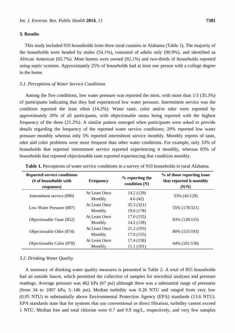
3. Results
This study included 910 households from three rural counties in Alabama (Table 1). The majority of
the households were headed by males (54.1%), consisted of adults only (90.9%), and identified as
African American (65.7%). Most homes were owned (92.1%) and two-thirds of households reported
using septic systems. Approximately 25% of households had at least one person with a college degree
in the home.
3.1. Perceptions of Water Service Conditions
Among the five conditions, low water pressure was reported the most, with more than 1/3 (35.3%)
of participants indicating that they had experienced low water pressure. Intermittent service was the
condition reported the least often (14.2%). Water taste, color and/or odor were reported by
approximately 20% of all participants, with objectionable tastes being reported with the highest
frequency of the three (21.2%). A similar pattern emerged when participants were asked to provide
details regarding the frequency of the reported water service conditions; 20% reported low water
pressure monthly whereas only 5% reported intermittent service monthly. Monthly reports of taste,
odor and color problems were more frequent than other water conditions. For example, only 33% of
households that reported intermittent service reported experiencing it monthly, whereas 83% of
households that reported objectionable taste reported experiencing that condition monthly.
Table 1. Perceptions of water service conditions in a survey of 910 households in rural Alabama.
Reported service conditions
(# of households with
responses)
Frequency % reporting the
condition (N)
% of those reporting issue
that reported it monthly
(N/N)
Intermittent service (890) At Least Once 14.2 (129)
33% (42/129) Monthly 4.6 (42)
Low Water Pressure (887) At Least Once 35.3 (321)
55% (178/321) Monthly 19.6 (178)
Objectionable Taste (852) At Least Once 17.0 (155)
83% (128/155) Monthly 14.2 (128)
Objectionable Odor (874) At Least Once 21.2 (193)
80% (155/193) Monthly 17.0 (155)
Objectionable Color (878) At Least Once 17.4 (158)
64% (101/158) Monthly 11.1 (101)
3.2. Drinking Water Quality
A summary of drinking water quality measures is presented in Table 2. A total of 855 households
had an outside faucet, which permitted the collection of samples for microbial analyses and pressure
readings. Average pressure was 462 kPa (67 psi) although there was a substantial range of pressures
(from 34 to 1007 kPa, 5–146 psi). Median turbidity was 0.26 NTU and ranged from very low
(0.05 NTU) to substantially above Environmental Protection Agency (EPA) standards (13.6 NTU).
EPA standards state that for systems that use conventional or direct filtration, turbidity cannot exceed
1 NTU. Median free and total chlorine were 0.7 and 0.9 mg/L, respectively, and very few samples
Page 7
Int. J. Environ. Res. Public Health 2014, 11 7382
lacked detectable chlorine (3.9% and 1.5%, respectively). Of the households tested, 16.7% and 12.2%
of outside and kitchen faucet samples, respectively, were positive for total coliforms. E. coli were
detected in less than 1% of water samples drawn from kitchen or outside faucets. All water quality
parameters, including turbidity, free and total chlorine, pressure and concentration of total coliforms or
E. coli, were non-normally distributed as determined by Shapiro-Wilk test of normality (p < 0.001)
and plots.
Table 2. Summary of drinking water quality measures for households using small rural
drinking water systems in Alabama.
Sample
Details
Water Quality Measures
Pressure
(kPa) **
Turbidity
(NTU)
Free
Chlorine
(mg/L)
Total
Chlorine
(mg/L)
Outside Total
Coliform
(MPN/100 mL)
Kitchen Total
Coliform
(MPN/100 mL)
Number of
Observations 855 887 802 802 855 890
Mean 462 0.37 0.90 * 1.1 * 5.7 3.8
Median 427 0.26 0.70 * 0.90 * <1 <1
Range 34–1000 0.050–14 <0.1–5.9 <0.1–6.2 <1–>200 <1–>200
% Below
Detection NA NA 3.9% 1.5% 83% 88%
Notes: * 88 observations from one research team member were excluded due to error in measurement for
both total and free chlorine; ** 1 kPa ≈ 0.145 psi.
3.3. Associations between Perceptions of Water Service Conditions and Measured Drinking
Water Quality
To determine whether or not reported problems surrounding water service delivery were associated
with measured water quality, we examined the five reported water service conditions (and their
frequency) for associations with the six water quality measures. A summary of these analyses is
presented in Tables 3 and 4. As shown for the analyses in these tables, statistically significant
associations were found between reported and measured water quality for two of the five reported
water service conditions: intermittent service and low water pressure.
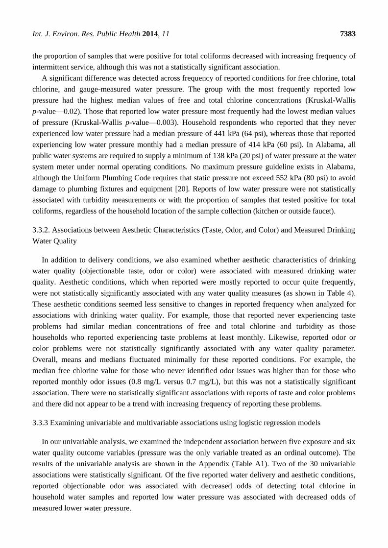
3.3.1. Associations between Water Delivery Conditions (Intermittent Service and Low Water Pressure)
and Measured Drinking Water Quality
As shown in Table 3, a significant difference was detected across frequency of reported intermittent
service and free and total chlorine. In this analysis, it was found that as the frequency of reported
intermittent service increased, so did the concentration of free and total chlorine (Kruskal-Wallis test
p-values 0.009 and 0.013 for free and total chlorine, respectively). No other water quality measures
were statistically significantly associated with increases in reported intermittent service although some
trends were noted. In particular, turbidity increased with increased reporting of intermittent service
while pressure decreased, but neither was statistically significant. Presence of total coliform bacteria
was variable depending upon the type of sample. For samples that were drawn from an outside faucet,
Page 8
Int. J. Environ. Res. Public Health 2014, 11 7383
the proportion of samples that were positive for total coliforms decreased with increasing frequency of
intermittent service, although this was not a statistically significant association.
A significant difference was detected across frequency of reported conditions for free chlorine, total
chlorine, and gauge-measured water pressure. The group with the most frequently reported low
pressure had the highest median values of free and total chlorine concentrations (Kruskal-Wallis
p-value—0.02). Those that reported low water pressure most frequently had the lowest median values
of pressure (Kruskal-Wallis p-value—0.003). Household respondents who reported that they never
experienced low water pressure had a median pressure of 441 kPa (64 psi), whereas those that reported
experiencing low water pressure monthly had a median pressure of 414 kPa (60 psi). In Alabama, all
public water systems are required to supply a minimum of 138 kPa (20 psi) of water pressure at the water
system meter under normal operating conditions. No maximum pressure guideline exists in Alabama,
although the Uniform Plumbing Code requires that static pressure not exceed 552 kPa (80 psi) to avoid
damage to plumbing fixtures and equipment [20]. Reports of low water pressure were not statistically
associated with turbidity measurements or with the proportion of samples that tested positive for total
coliforms, regardless of the household location of the sample collection (kitchen or outside faucet).
3.3.2. Associations between Aesthetic Characteristics (Taste, Odor, and Color) and Measured Drinking
Water Quality
In addition to delivery conditions, we also examined whether aesthetic characteristics of drinking
water quality (objectionable taste, odor or color) were associated with measured drinking water
quality. Aesthetic conditions, which when reported were mostly reported to occur quite frequently,
were not statistically significantly associated with any water quality measures (as shown in Table 4).
These aesthetic conditions seemed less sensitive to changes in reported frequency when analyzed for
associations with drinking water quality. For example, those that reported never experiencing taste
problems had similar median concentrations of free and total chlorine and turbidity as those
households who reported experiencing taste problems at least monthly. Likewise, reported odor or
color problems were not statistically significantly associated with any water quality parameter.
Overall, means and medians fluctuated minimally for these reported conditions. For example, the
median free chlorine value for those who never identified odor issues was higher than for those who
reported monthly odor issues (0.8 mg/L versus 0.7 mg/L), but this was not a statistically significant
association. There were no statistically significant associations with reports of taste and color problems
and there did not appear to be a trend with increasing frequency of reporting these problems.
3.3.3 Examining univariable and multivariable associations using logistic regression models
In our univariable analysis, we examined the independent association between five exposure and six
water quality outcome variables (pressure was the only variable treated as an ordinal outcome). The
results of the univariable analysis are shown in the Appendix (Table A1). Two of the 30 univariable
associations were statistically significant. Of the five reported water delivery and aesthetic conditions,
reported objectionable odor was associated with decreased odds of detecting total chlorine in
household water samples and reported low water pressure was associated with decreased odds of
measured lower water pressure.
Page 9
Int. J. Environ. Res. Public Health 2014, 11 7384
Table 3. Association between reported intermittent service and low water pressure and measured water quality in a sample of households of
three rural counties in Alabama 2012.
Water Delivery
Condition Frequency
Median Free Cl
mg/L (N)
Median Total Cl
mg/L (N)
Median Turbidity
NTU (N)
Median Pressure
kPa # (N)
Kitchen Total Coliform (%
positive in 100 mL)
Outside Total Coliform (%
positive in 100 mL)
Intermittent
Service
Never 0.7 (673) 0.9 (673) 0.26 (741) 441 (715) 12.1% 16.9%
At Least Once 1.0 (75) 1.2 (75) 0.27 (84) 434 (82) 11.8% 15.9%
At Least Monthly 1.5 (35) 1.5 (35) 0.34 (42) 469 (39) 16.8% 15.0%
p-Value 0.009 * 0.013 * 0.22 * 0.42 * 0.65 † 0.94 †
Low Water
Pressure
Never 0.7 (497) 0.9 (497) 0.27 (549) 441 (528) 12.5% 18.4%
At Least Once 0.8 (122) 0.9 (122) 0.23 (142) 441 (139) 12.7% 11.6%
At Least Monthly 0.9 (163) 1.1 (163) 0.27 (174) 414 (167) 10.3% 15.9%
p-Value 0.02 * 0.02 * 0.06 * 0.003 * 0.71† 0.15 †
Notes: * Compared with Kruskal-Wallis test; † Proportion tested with Pearson Chi-square test; Statistically significant differences in bold; # 1 kPa ≈ 0.145 psi.
Table 4. Association between reported taste, odor and color issues and measured water quality in a sample of households of three rural
counties in Alabama 2012.
Aesthetic
Characteristic Frequency
Median Free Cl
mg/L (N)
Median Total Cl
mg/L (N)
Median Turbidity
NTU (N)
Median Pressure
kPa # (N)
Kitchen Total Coliform (%
positive in 100 mL)
Outside Total Coliform (%
positive in 100 mL)
Objectionable
Taste
Never 0.8 (578) 0.9 (578) 0.26 (643) 441 (615) 13.0% 17.2%
At Least Once 0.9 (36) 1.0 (36) 0.23 (38) 414 (37) 2.63% 23.7%
At Least Monthly 0.8 (140) 0.9 (140) 0.27 (150) 427 (149) 11.9% 12.8%
p-Value 0.37 * 0.58 * 0.57 * 0.70 * 0.16 † 0.22 †
Objectionable
Odor
Never 0.8 (628) 0.9 (628) 0.26 (700) 427 (674) 12.2% 16.4%
At Least Once 0.9 (23) 1.2 (23) 0.24 (27) 482 (25) 11.1% 19.2%
At Least Monthly 0.7 (119) 0.8 (119) 0.28 (127) 441 (124) 12.5% 16.7%
p-Value 0.69 * 0.42 * 0.53 * 0.61 * 0.98 † 0.89 †
Objectionable
Color
Never 0.8 (637) 0.9 (639) 0.27 (703) 427 (677) 11.5% 15.9%
At Least Once 0.9 (49) 1.0 (49) 0.22 (55) 469 (53) 19.6% 17.0%
At Least Monthly 0.7 (87) 0.9 (87) 0.24 (99) 441 (99) 13.1% 20.8%
p-Value 0.81 * 0.85 * 0.16 * 0.48 * 0.19† 0.48 †
Notes: * Medians compared with Kruskal-Wallis test; † Proportion tested with Pearson Chi-square test; # 1 kPa ≈ 0.145 psi.
Page 10
Int. J. Environ. Res. Public Health 2014, 11 7385
Due to collinearity of the exposure variables, all multivariable models included one binary exposure
variable (intermittent service, low water pressure, objectionable taste, odor or odd color) and three
confounding variables—access to sewerage, presence of college graduates in the household and
reported race—for each binary water quality measure or for the ordinal water pressure measure. There
were no significant interactions between confounders and exposures, therefore only the main effects
are reported. To simplify the presentation, all adjusted models are included in Table 5. The ten models
that were found to have >10% change in effect when the three confounding variables were included in
the model are indicated in the table. The other 20 models did not demonstrate a significant change in
effect when the confounding variables were included. Overall, the results of this analysis were similar
to the results of the univariable analysis. Two of the 30 associations examined remained statistically
significant in the multivariable analysis. Households that reported an odor problem had decreased odds
of total chlorine detected in the samples (OR =0.21, 95% CI (0.060–0.77)) and households that
reported low water pressure had increased odds (OR =1.40, 95% CI (1.07–1.84)) of measured low
water pressure (using the proportional odds model).
Table 5. Multivariable regression examining association between reported delivery and
aesthetic conditions, sewerage and measured water quality in a sample of households of
three rural counties in Alabama 2012.
Reported
delivery and
aesthetic
conditions
Presence of total
coliforms in
kitchen samples
OR (95%CI)
Presence of total
coliforms in
outside samples
OR (95%CI)
Presence of
free chlorine
OR (95%CI)
Presence of total
chlorine
OR (95%CI)
Turbidity
> 0.3NTU
OR (95%CI)
Log-transformed
Pressure Quintiles*
OR (95% CI)
Intermittent
Service 0.99 (0.55–1.8) † 0.82 (0.47–1.4)† 2.2 (0.50–9.4) 0.69 (0.14–3.3) † 1.45 (0.92–2.0) 0.98 (0.66–1.5) †, ‡
Low Water
Pressure 0.78 (0.50–1.2) † 0.73 (0.49–1.1) 0.94 (0.44–2.1) 2.5 (0.51–12) † 0.76 (0.57–1.0) 1.4 (1.1–1.8)
Objectionable
Taste 0.82 (0.48–1.4) 0.80 (0.50–1.3) 0.99 (0.41–2.4) 0.29 (0.080–1.1) † 0.94 (0.67–1.3) 1.1 (0.82–1.5)
Objectionable
Odor 1.0 (0.59–1.8) 1.17 (0.66–1.7) 0.92 (0.37–2.3) 0.21 (0.060–0.77)
† 0.98 (0.68–1.4) 0.94 (0.67–1.3)
Objectionable
Color 1.6 (0.95–2.6) † 1.36 (0.78–2.0) 1.5 (0.50–4.4) 0.93 (0.19–4.5) † 0.77 (0.53–1.1) 0.99 (0.70–1.4)
Notes: * Ordinal logistic regression performed on quintiles of log-transformed pressure; † indicates
multivariable model produced ≥10% change in effect size of exposure variable ‡ Logistic regression
performed on binary log-pressure when proportional odds assumption was not met; Statistically significant
results in bold.
4. Discussion
The results of this study were used to evaluate consumers’ perceptions of the delivery and aesthetics
of drinking water from small water systems, and how those perceptions were associated with chlorine,
turbidity, and microbiological water quality measured at the household. We examined five service
conditions: two focused on the level of service delivery, including water pressure and intermittent
service, and three focused on the aesthetic conditions of taste, odor and color. Overall, we found few
Page 11
Int. J. Environ. Res. Public Health 2014, 11 7386
statistically significant associations between these reported conditions and analyzed parameters for
drinking water quality.
4.1. Self-Reported Water Delivery Conditions
There is an increasing recognition of the role that drinking water distribution systems may play in
infectious disease outbreaks and even endemic disease transmission [21]. It is important for drinking
water distribution systems to maintain hydraulic integrity to protect the water from external
contaminants. The Committee on Public Water Supply Distribution Systems of the National Research
Council defines hydraulic integrity as the capacity to maintain desirable water flow, water pressure,
and water age in a distribution system [22]. For this study, we focused on consumer self-reporting of
the system’s ability to maintain a desirable water flow and water pressure paired with a single
measurement of pressure at each household.
Our data indicated that 35.3% of participants reported experiencing low water pressure, which is
a documented risk factor for outbreaks of waterborne disease [23]. There are many causes of low water
pressure events, including main breaks, opening and closing of valves, power failures, flushing of the
system, turning pumps on or off, fighting fires, and any other event that creates a sudden change in
water pressure. These low-pressure events can last from minutes to hours. Hydraulic integrity relies on
the maintenance of adequate water pressure in a distribution system. Loss of water pressure can
represent a breach within the system that could result in either backflow (from cross-connections) or
contaminant intrusion [24].
Intermittent service was reported less frequently than low water pressure; however, 15% of our
participants reported experiencing this condition at least once. For our study, intermittent service was
defined as an interruption in water service provided to households for any length of time. Interruption in
service is associated with infiltration events, stagnation, and potential growth of microbiological
contaminants. Distribution systems with intermittent water supply are most vulnerable to intrusion events,
and developing countries are more likely to suffer from intermittent water supplies [25]. Under these
circumstances, the risk for contamination is high, with several reports of waterborne disease outbreaks and
increased rates of gastrointestinal illness linked to intermittent service [26,27]. In economically richer
countries, intermittent supply is less common, but these events still occur in locations where infrastructure
function is sub-optimal. Previous research conducted in our study area asked households connected to the
water supply system about their perceptions of water system performance. Of those participating, 37% of
consumers said that they experienced problems with their connection, most commonly intermittent service,
while 14% of all participants reported service interruptions as a recurring issue [16].
4.2 Prevalence of Self-Reported Aesthetic Conditions
Households in our study reported various concerns about drinking water aesthetics, with almost
20% of households experiencing some problem with taste, odor and/or color. From a previous study
conducted in the area, 18% of public water users rated the color of their water as ―poor‖ or ―very
poor‖, and 12% rated the taste of their water as ―poor‖ or ―very poor‖ [16]. Additionally, a study in
Norway documented equivalent or higher percentages of households who reported similar concerns
(approximately 30% for taste and odor and 15% for rusty color) [28]. A USA-based study determined
Page 12
Int. J. Environ. Res. Public Health 2014, 11 7387
that the most important reason for consumers to preferentially consume bottled water over tap water
was because they did not like the taste/odor of the water [29]. Multiple other studies have
demonstrated that perceived aesthetic values such as color, odor, and taste associated with public
drinking water supplies are common reasons for seeking alternatives [30–34].
4.3. Chlorine Residuals
Maintenance of a disinfectant residual throughout the distribution system helps to preserve the
integrity of the system by inactivating microorganisms, indicating system problems, and controlling the
growth of biofilms. The EPA-recommended range for free chlorine residual at the household level is
0.3–0.5 mg/L [35]. If free residual chlorine levels are non-detectable at the household level, it is assumed
that the water supply is not protected against recontamination. Our data showed the median free chlorine in
our samples was 0.7 mg/L, and very few samples (<2%) had no detectable chlorine. The use of chlorine for
disinfection of drinking water may produce a bleach-like odor and/or taste, however, the ability of the
consumer to detect this residual varies. EPA has not set a standard for these aesthetic effects, but instead
established a maximum residual disinfectant level of 4 mg/L for chlorine that is capable of preventing
physiological health effects, such as eye and nose irritation and stomach discomfort. Bacterial
contamination was infrequent, with 13-16% of both outside and kitchen faucet samples having detectable
total coliforms. The results from this study suggested that the measured microbiological water quality from
these households was slightly better than what was detected in a previous study in the area. That study
reported a higher percentage of samples with no detectable free chlorine, greater than 33% (N = 305), and
almost 10% of public water system samples were positive for fecal coliforms [16].
4.4. Associations between Low Pressure, Intermittent Service and Water Quality
In our initial analysis, higher reported frequencies of low water pressure and intermittent service were
associated with increased free and total chlorine but not associated with the presence of total coliforms. It
is possible that when the utilities experience these conditions, they attempt to correct the problem by
adding additional chlorine. This may be the reason that we saw a decrease in the percentage of samples
positive for total coliforms when low water pressure and intermittent service were reported. When we
performed univariate and multivariable logistic regression (examining only the presence of chlorine and
not the concentration), there was not a statistically significant association between frequency of report of
intermittent service or low water pressure and the presence of free or total chlorine in water samples.
Reported low water pressure was associated with lower measured water pressure. We found this in
our initial analysis and also in univariable and multivariable regression analyses. Few studies have
examined pressure at the household level, but low pressure could also be associated with increased
opportunities for intrusion into pipes. A case study in the United Kingdom found a very strong
association between reported low water pressure at the tap and self-reported diarrhea [36]. From these
results, the authors concluded that up to 15% of the gastrointestinal illness (GI) reported among the
exposed individuals may be associated with burst water mains and pressure loss events, although the
study was not specifically designed to test the hypothesis that low water pressure events were
associated with self-reported diarrhea. Additionally, a Norwegian epidemiological study indicated that
low pressure episodes (defined as incidents where a part of the water distribution network was closed
Page 13
Int. J. Environ. Res. Public Health 2014, 11 7388
off due to main breaks or maintenance work with presumed loss of water pressure in the distribution
system) caused an increased risk of GI illness among water recipients [37]. A study in the USA
suggested a mechanism for this increased GI illness by showing that when otherwise satisfactory water
distribution pipes experienced a low pressure event, they aspirated enteric organisms that were present
in the soil surrounding the pipe [38]. Similarly, a recent study in India reported that households with
intermittent service as opposed to continuous supply were more likely to detect E. coli and have lower
chlorine residual values [5]. Thus, the high prevalence of reported low water pressure and its
association with decreased measured pressure in our study group is a cause for concern given this
potential for increased disease risk.
4.5. Associations between Aesthetic Conditions and Water Quality
In our preliminary analysis of reported aesthetic conditions and water quality in this setting,
we found no statistically significant associations between these and other variables we measured.
When we examined the associations using univariable and multivariable techniques, we found
a statistically significant association with reported odor problems and decreased odds of detecting total
chlorine in the water samples. We emphasize that human perception and perception data are complex,
and our measures may not have captured aesthetic characteristics that could be assumed to have
a meaningful association with microbial risk. For example, color can result from different types of
contaminants (e.g., rust, sediment) that may not correlate well with other measures of water quality.
Furthermore, if a household reported poor taste and odor, they often considered it to occur frequently.
Perhaps frequently reported taste and odor problems are an indication of general dislike of the water
provided by the small water system, and reflect a more general complaint about the quality of service.
As a result, the frequency with which these conditions are reported may be less sensitive to actual
fluctuations in aesthetic properties of the water. Additionally, aesthetic characteristics are highly
subject to variability in what each individual may consider to be undesirable, suggesting that what
one individual may find distasteful or aesthetically unpleasing may not bother another person.
Further confounding the issue, the threshold for taste and odor varies with the contaminant of concern,
adding even more variability. These complexities have been well documented [39]. As a previous
study conducted in the region did not find associations between consumer reported intensity
of water condition and water contamination [16], this study focused on overall perceptions
(i.e., non-scaled responses).
Previous studies have suggested that aesthetic characteristics are associated with user perception of
risk [10,28]. A study that surveyed residents of two community water systems determined that water
contamination problems contributed to increased levels of risk perception from those individuals
drinking tap water [29]. They also suggested that the level of awareness of the problem affected risk
perception [29]. When the utility was unable to correct the condition in a timely manner, the
consumer’s perception of risk increased [29]. Limited to a single sample at each household and
looking into general perception measurements, our results suggest limited association between
perceptions and objectively measurable factors that are known to be associated with microbial risk in
this setting. Our approach limits the ability to provide exact links to these perceptions but our intention
was to provide a more general sense of how the consumers felt about the water and evaluate the water
quality at a single point in time. Furthermore, water quality measures were taken only once for
each household and single samples are insufficient as indicators of long-term water quality in
water supplies.
Page 14
Int. J. Environ. Res. Public Health 2014, 11 7389
5. Conclusions
Data from this study support the following primary conclusions: (1) self-reported aesthetic data from
consumers were found to have no or limited associations with measured water quality parameters that are
known to be associated with microbial risk (pressure, turbidity, chlorine residuals, total coliforms);
(2) self-reported pressure data were associated with measured pressure at the household level, indicating
that self-reported data on this parameter may be reliable; and (3) reported low water pressure and
intermittent service were associated with elevated free and total chlorine concentrations measured at the
point of sampling but had limited association with presence or absence of these residuals.
Acknowledgments
This publication was developed under Assistance Agreement No. R834866 awarded by the U.S.
Environmental Protection Agency (EPA) to the University of Alabama (Johnson and Brown, PIs). This
paper has not been formally reviewed by EPA. The views expressed in this document are solely those
of the authors and do not necessarily reflect those of the Agency. EPA does not endorse any products
or commercial services mentioned in this publication. We would like to thank the following members
of our Data Collection Team: Daniel Bunei, Tabatha Dye, Gabrielle Hance, Bailie Clark,
Alesia Tubbs, Davida Reeves, and Moses Hopson. We would also like to thank Tracy Ayers for her
review and contribution to the statistical analyses.
Author Contributions
Jessica C. Wedgworth maintained all databases for this project, assisted with field collection of the
data, and was the primary author of this manuscript. Joe Brown was a co-investigator on the project,
developed the sampling protocol, and assisted with manuscript preparation. Pauline Johnson was the
lead project investigator, oversaw the field research team, and assisted with manuscript preparation.
Julie B. Olson was a co-investigator on the project and assisted with manuscript preparation.
Christine E. Stauber contributed to research design, data analysis, and writing of the manuscript.
Rick Forehand assisted with data collection. Mark Elliott assisted with manuscript preparation.
Conflicts of Interest
The authors declare no conflict of interest.
References
1. Eskaf, S.; Nida, C.; Hughes, J. Results of the 2010 North Carolina Water and Wastewater Financial
Practices and Policies Survey. UNC Environmental Finance Center: Chapel Hill, NC, USA, 2011.
2. Eskaf, S. EPA’s 2011 SDWIS Data Analyzed by the Environmental Finance Center at the
University of North Carolina. In Proceedings of the 2012 Water and Health Conference, Chapel
Hill, NC, USA, 29 October, 2 November 2012.
3. Sobsey, M.D. Drinking water and health research: a look to the future in the United States and
globally. J. Water Health 2006, 4, 17–21.
Page 15
Int. J. Environ. Res. Public Health 2014, 11 7390
4. Impellitteri, C.; Patterson, C.L.; Haught, R.C.; Goodrich, J.A. Small Drinking Water Systems:
State of the Industry and Treatment Technologies to Meet the Safe Drinking Water Act
Requirements; EPA/600/R-07/110; National Risk Management Research Laboratory, Office of
Research and Development, USEPA: Cincinnati, OH, USA, 2007.
5. Kumpel, E.; Nelson, K.L. Comparing microbial water quality in an intermittent and continuous
piped water supply. Water Res. 2013, 47, 5176–5188.
6. The Safe Drinking Water Information System (SDWIS). Available online: http://www.epa.gov/
enviro/ facts/sdwis/search.html. (accessed on 23 February 2014).
7. Reynolds, K.A.; Mena, K.D.; Gerba, C.P. Risk of waterborne illness via drinking water in the
United States. Rev. Environ. Contam. Toxicol. 2008, 192, 117–158.
8. Payment, P.; Richardson, L.; Semiatucki, J.; Dewar, R.; Edwards, M.; Franco, E. A randomized
trial to evaluate the risk of gastrointestinal disease due to consumption of drinking water meeting
current microbiological standards. Am. J. Public Health 1991, 81, 703–708
9. Payment, P.; Siemiatucki, J.; Richardson, L.; Renaud, G.; Franco, E.; Prevost, M. A prospective
study of gastrointestinal health effects due to consumption of drinking water. Int. J. Environ.
Health Res. 1997, 7, 5–31.
10. Doria, M.F.; Pidgeon, N.; Hunter, P.R. Perceptions of drinking water quality and risk and its
effect on behaviour: A cross-national study. Sci. Total Environ. 2009, 407, 5455–5464.
11. Roche, S.M.; Jones-Bitton, A.; Majowicz, S.E.; Pintar, K.D.; Allison, D. Investigating public
perceptions and knowledge translation priorities to improve water safety for residents with private
water supplies: A cross-sectional study in Newfoundland and Labrador. BMC Publ. Health 2013,
13, doi:10.1186/1471-2458-13-1225.
12. Arnold, M.; VanDerslice, J.A.; Taylor, B.; Benson, S.; Allen, S.; Johnson, M.; Kiefer, J.; Boakye,
I.; Arhinn, B.; Crookston, B.T.; Ansong, D. Drinking water quality and source reliability in rural
Ashanti region, Ghana. J. Water Health 2013, 11, 161–172.
13. Orgill, J.; Jeuland, A.; Brown, J.; Shaheed, A. Water quality perceptions and willingness to pay
for clean water in peri-urban Cambodian communities. J. Water Health 2013, 11, 489–506.
14. Wimberley, R.; Morris, L. The regionalization of fever, assistance for the Black Belt south?
J. Rural Soc. Sci. 2002, 18, 294–306.
15. Lichtenstein, B. Illicit drug use and the social context of HIV/AIDS in Alabama’s black belt.
J. Rur. Health 2007, 23, 68–72.
16. Wedgworth, J.C.; Brown, J. Limited access to safe drinking water and sanitation in Alabama’s
Black Belt: A cross-sectional case study. Water Qual. Expos. Health 2012, 5, 69–74.
17. He, J.; Dougherty, M.; Zellmer, R.; Martin, G. Assessing the status of onsite wastewater treatment
systems in the Alabama Black Belt soil area. Environ. Eng. Sci. 2011, 28, 693–699.
18. Clesceri, L.; Baird, R.; Rice, E.; Eaton, A. Standard Methods for the Examination of Water and
Wastewater, 2nd Ed.; American Public Health Association: Washington, DC, USA, 2012.
19. New England Water Works Association (NEWWA). Pocket Sampling Guide for Operators of
Small Water Systems; NEWWA: Holliston, MA, USA, 2004.
20. Alabama Department of Environmental Management (ADEM). Water Supply Program; Admin.
Code r. 335-7-x-.xx. Revised Effective 27 November 272012; ADEM: Montgomery, AL, USA,
2012.
21. Ercumen, A.; Gruber, J.S.; Colford, J.M. Water distribution system deficiencies and gastrointestinal
illness: A systematic review and meta-analysis. Environ. Health Perspect. 2014, 122, 651–660.
Page 16
Int. J. Environ. Res. Public Health 2014, 11 7391
22. National Research Council (NRC). Drinking Water Distribution Systems: Assessing and Reducing
Risks; National Academies Press: Washington, DC, USA, 2006.
23. Hunter, P.R. Waterborne disease: epidemiology and ecology; Wiley: Chinchester, UK, 1997.
24. Kirmeyer, G.J.; Martel, K. Pathogen Intrusion into the Distribution System; American Water
Works Association: Denver, CO, USA, 2001.
25. Tinker, S.; Moe, C.; Klein, M.; Flanders, W.; Uber, J.; Amirtharajah, A.; Singer, P.; Tolbert, P.
Drinking water residence time in distribution networks and emergency department visits for
gastrointestinal illness in Metro Atlanta, Georgia. J. Water Health 2009, 7, 332–343
26. Swerdlow, D.L.; Woodruff, B.A.; Brady, R.C.; Griffin, P.M.; Tippen, S.; Donnell, H.D.;
Geldreich, E.; Payne, B.J.; Meyer, J.; Wells, J.G.; Greene, K.D.; et al. A waterborne outbreak in
Missouri of Escherichia coli O157: H7 associated with bloody diarrhea and death. Ann. Intern.
Med. 1992, 117, 812–819.
27. Mermin, J.H.; Villar, R.; Carpenter, J.; Roberts, L.; Gasanova, L.; Lomakina, S.; Bopp, C.;
Hutwagner, L.; Mead, P.; Ross, B.; et al. A massive epidemic of multidrug-resistant typhoid fever
in Tajikistan associated with consumption of municipal water. J. Infect. Dis. 1999, 179, 1416–1422.
28. Duponte, D.; Krupnick, A. Differences in water consumption choices in Canada: the role of
socio-demographics, experiences, and perceptions of health risks. J. Water Health 2010, 8, 671–686.
29. Anadu, E.C.; Harding, A.K. Risk perception and bottled water use. J. Am. Water Works Assoc.
2000, 92, 82–92.
30. Auslander, B.A.; Langlois, P.H. Toronto tap water: Perception of its quality and use of
alternatives. Can. J. Publ. Health 1992, 84, 99–102.
31. Levallois, P.; Grondin, J.; Gingras, S. Evaluation of consumer attitudes on taste and tap water
alternatives in Quebec. Water Sci. Technol. 1999, 40, 135–139.
32. Kleczyk, E.J.; Bosch, D.J.; Dwyer, S.; Lee, J.; Loganathan, G.V. Maryland Home Drinking Water
Assessment. In Proceedings of the 2005 Virginia Water Research Symposium, Blacksburg, VA,
USA, October 10–12, 2005; pp. 104–113.
33. Doria, M.F. Bottled water vs. tap water: Understanding consumers’ preferences. J. Water Health
2006, 4, 271–276.
34. Hu, Z.; Morton, L.W.; Mahler, R.L. Bottled water: United States consumers and their perceptions
of water quality. Int. J. Environ. Res. Public Health 2011, 8, 565–578.
35. United States Environmental Protection Agency (USEPA). National Primary Drinking Water
Regulations. Code of Federal Regulations, 40 CFR Part 141; USEPA: Washington, DC, USA.
36. Hunter, P.R.; Chalmers, R.M.; Hughes, S.; Syed, Q. Self-Reported diarrhea in a control group:
A strong association with reporting of low-pressure events in tap water. Clin. Infect. Dis. 2005,
40, 32–34.
37. Nygård, K.; Wahl, E.; Krogh, T.; Tveit, O.A.; Bøhleng, E.; Tverdal, A.; Aavitsland, P. Breaks and
maintenance work in the water distribution systems and gastrointestinal illness: A cohort study.
Int. J. Epidemiol. 2007, 36, 873–880.
38. LeChevallier, M.W.; Gullick, R.; Karim, M.; Friedman, M.; Funk, J. The potential for health risks
from intrusion of contaminants into the distribution system from pressure transients. J. Water
Health 2003, 1, 3–14
39. Rao, Y.R.; Skafel, M.G.; Howell, T.; Murthy, R.C. Physical processes controlling taste and odor
episodes in Lake Ontario drinking water. J. Great Lakes Res. 2003, 29, 70–78.
Page 17
Int. J. Environ. Res. Public Health 2014, 11 7392
Appendix
Table A1. Univariable associations between reported delivery and aesthetic conditions and measured water quality in a sample of households
of three rural counties in Alabama 2012.
Reported delivery
and aesthetic
conditions
Presence of total
coliforms in kitchen
samples
OR (95%CI)
Presence of total
coliforms in outside
samples
OR (95%CI)
Presence of free
chlorine
OR (95%CI)
Presence of total
chlorine
OR (95%CI)
Turbidity > 0.3
NTU
OR (95%CI)
Log-transformed
Pressure Quintiles * OR
(95% CI)
Intermittent Service 1.12 (0.64–1.95) 0.92 (0.54–1.56) 2.25 (0.53–9.63) 0.81 (0.17–3.76) 1.36 (0.93–1.99) 0.89 (0.59–1.34) ‡
Low Water Pressure 0.89 (0.58–1.37) 0.71 (0.49–1.06) 1.04 (0.49–2.21) 2.94 (0.63–13.34) 0.78 (0.59–1.04) 1.43 (1.10–1.85)
Objectionable Taste 0.75 (0.44–1.26) 0.85 (0.54–1.34) 1.00 (0.42–2.37) 0.42 (0.13–1.33) 0.98 (0.70–1.36) 1.11 (0.82–1.49)
Objectionable Odor 1.00 (0.59–1.70) 1.11 (0.70–1.76) 0.94 (0.38–2.33) 0.31 (0.10–0.99) 1.02 (0.72–1.46) 0.95 (0.68–1.32)
Objectionable Color 1.41 (0.86–2.31) 1.27 (0.81–2.01) 1.46 (0.50–4.24) 1.07 (0.23–4.93) 0.78 (0.54–1.12) 0.97 (0.70–1.35)
Note: * Ordinal logistic regression performed on quintiles of log-transformed pressure. Odds ratios derived from modeling the probability of being in a lower level of
pressure are reported; ‡ Logistic regression performed on binary pressure when proportional odds assumption was not met; Statistically significant results in bold.
© 2014 by the authors; licensee MDPI, Basel, Switzerland. This article is an open access article distributed under the terms and conditions of the Creative
Commons Attribution license (http://creativecommons.org/licenses/by/3.0/).