Tractable Models and Algorithms

for Assortment Planning with Product Costs

Sumit Kunnumkal∗ • Victor Martınez-de-Albeniz†

Submitted: January 21, 2016. Revised: July 27, 2017.

Abstract

Assortment planning under a logit demand model is a difficult problem when there areproduct-specific fixed costs. We develop a new continuous relaxation of the problem that isbased on the parametrization of the problem on the total assortment attractiveness. Thisrelaxation provides an upper bound on the optimal expected profit. We show that the upperbound can be computed efficiently and allows us to generate feasible solutions with attractiveperformance guarantees. We analytically prove that these are close to optimal when products arehomogeneous in terms of preference weights. Moreover, our formulation can be easily extendedto incorporate additional constraints on the assortment, or multiple customer segments. Finally,we provide numerical experiments that show that our method yields tight upper bounds andperforms competitively with respect to other approaches found in the literature.

1 Introduction

The optimization of assortment plans is an important problem for most retailers. In the very broad

literature on this topic, product fixed costs have been identified as one of the drivers that make

optimization difficult. In practice, these costs may arise from store or shelf preparation costs. They

may be very significant, especially for slow movers, even when they have high margins. For instance,

in the soft drinks category of a supermarket, these costs may vary with the product type, by a

factor 1 (small items that do not consume much space in the store and are easy to handle) to 20

(large volume items). In this example, about half of the products in the assortment should only sell

1 unit per week to recoup the fixed cost, the other half of the products should sell more (some must

sell at least 1 per day to recover it). Furthermore, in situations where product assortments change

often (e.g., for stores selling new phones or apparel, see Caro and Martınez-de Albeniz 2015), the

consideration of fixed costs is even more important, because they need to be recovered in a short

time.

∗Smith School of Business, Queen’s University, Kingston K7L2G8, Canada, email: sk162@queensu.ca†IESE Business School, University of Navarra, Av. Pearson 21, 08034 Barcelona, Spain, email: valbeniz@iese.edu.

V. Martınez-de-Albeniz’s research was supported in part by the European Research Council - ref. ERC-2011-StG283300-REACTOPS and by the Spanish Ministry of Economics and Competitiveness (Ministerio de Economıa yCompetitividad) - ref. ECO2014-59998-P.

1

Besides being an important problem in its own right, the assortment model with fixed costs

appears in a number of other contexts. For example, assortment optimization with constraints is

difficult in general and one approach to obtain tractable models is to dualize the difficult constraints

by associating Lagrange multipliers with them. The resulting relaxation has precisely the same

form as the fixed costs problem if we interpret the Lagrange multipliers as the product fixed costs.

One example of this approach is Feldman and Topaloglu (2015), who consider the assortment

optimization problem when demand follows the mixture of multinomial models (MMNL): to solve

it, they develop a relaxation in the form of an assortment problem with product fixed costs. The

assortment model with fixed costs also has applications to choice revenue management. The choice

revenue management problem can be viewed as solving a sequence of assortment problems that

are linked together by resource constraints. Kunnumkal and Topaloglu (2008) dualize the resource

capacity constraints and the sub-problems in their method end up being assortment optimization

problems with fixed costs.

In this paper, we consider assortment planning under a multinomial logit (MNL) demand model

where products involve fixed costs, together with different margins and attractiveness (preference

weights). The objective in our approach is to maximize the expected profit, i.e., the expected sales

contribution margin minus fixed assortment costs. The resulting optimization problem is known to

be NP-hard (Kunnumkal et al. 2009). To circumvent this difficulty, we develop a tractable relax-

ation of the assortment optimization problem that is based on a parametric continuous knapsack

formulation. We use the total attractiveness of the assortment including the attractiveness of the

no-purchase option as a parameter in our relaxation. Our relaxation involves (1) solving a con-

tinuous knapsack problem for each value of the total attractiveness parameter, and (2) selecting

the best possible value of the parameter. This process generates an upper bound on the optimal

expected profit.

Upper bounds are useful in assessing the sub-optimality of heuristic assortments. Hence, tighter

upper bounds are more valuable since they provide a more accurate assessment of the optimality

gap. They also allow us to generate feasible solutions with attractive performance.

Our approach yields a number of useful results. We first prove that the upper bound can be

obtained efficiently. In particular, we show that the best possible value of the total attractiveness

parameter, and hence the upper bound can be obtained in polynomial time, namely O(n3) where

n is the total number of products available.

In addition, our upper bound is provably tighter than the existing bounds in the literature. We

2

provide an analytical characterization of the gap between optimal expected profit and our upper

bound. Specifically, we show that the upper bound obtained by our relaxation is never more than

twice that of the optimum. To our knowledge, the existing bounds in the literature lack such

theoretical guarantees. In addition, we construct a family of assortment problems which shows

that the worst-case gap of 2 is in fact tight. We find that the worst-case gap is achieved when

one product is significantly different than the rest in terms of margins and attractiveness. This

situation may not occur very frequently in practice especially when we think of the products as

being potential substitutes. When the characteristics of the products are more similar, we obtain a

sharper characterization of the gaps between our upper bound and the optimal expected profit. We

show that the gap is within a factor of 3/2 without making strong assumptions on the parameter

space. Furthermore, when the number of products is large, then we show that the gap is quite

close to zero. An appealing feature of our analysis is that the gap is a simple function of only

the product attractiveness parameters and is independent of the profit margins and the product

fixed costs. The sharper characterizations of the gap are more likely to be applicable in many

practical situations and are thus useful in providing a more realistic picture of the performance of

our method. To validate these insights, in our computational study we find that our relaxation

generally obtains bounds that are very close to optimal, with average optimality gaps below 1%

and worst-case gaps of a few percentage points. Also, as a useful by-product from the proof of the

upper bound’s gap performance, we are able to generate feasible assortments that perform close to

optimal: this heuristic thus provides very competitive performance at a reasonable computational

cost.

Finally, by taking a novel dual perspective, we extend the relaxation idea to incorporate addi-

tional modelling elements. We show that incorporating general linear constraints on the assortment

and multiple customer classes (i.e., a mixture of multinomial logit models) still allows us to calcu-

late the upper bound by minimizing a finite number of functions. It turns out that the number of

functions to consider is of order O(

nD+E)

where D is the number of customer classes and E the

number of constraints. So it is only useful when the number of classes and constraints is small.

These results can be extended further when there is a single customer class, in which case we show

that the complexity of obtaining the upper bound is O(

n3(1+E))

. When there are constraints on

the assortment, we cannot obtain guarantees on the performance of our heuristic in general. How-

ever, we are able to recover the performance guarantee of 2 for some classes of constraints that are

common in the assortment literature: (1) cardinality constraints which limit the total number of

3

products offered and (2) product precedence constraints which require that a certain set of products

be included in the assortment if a given product is part of the assortment.

Our results thus advance the understanding of assortment planning with product fixed costs.

We make three main contributions to the literature. First, we build on Kunnumkal et al. (2009)

to obtain a new, tractable upper bound on the optimal expected profit. Second, we show that

our upper bound has attractive theoretical guarantees. It is provably tighter than the existing

bounds in the literature and we are able to analytically characterize the gap between our upper

bound and the optimal expected profit. Our analysis provides insight into when our upper bound

is tight. We find that irrespective of the profit margins and product fixed costs, the gap between

the optimal profit and our upper bound is small as long as the product preference weights are not

very different. Our computational study further indicates that the feasible solution obtained from

the computation of the upper bound has very competitive performance. Our analytical results

explain the good practical performance of this heuristic to a large extent. And third, our approach

can be applied to more difficult problems that include constraints on the assortment and multiple

customer classes, as demonstrated both analytically and through our numerical study.

The rest of the paper is organized as follows. Section 2 reviews the related literature. Section 3

formulates the problem and Section 4 develops the continuous relaxation and the heuristic. Section

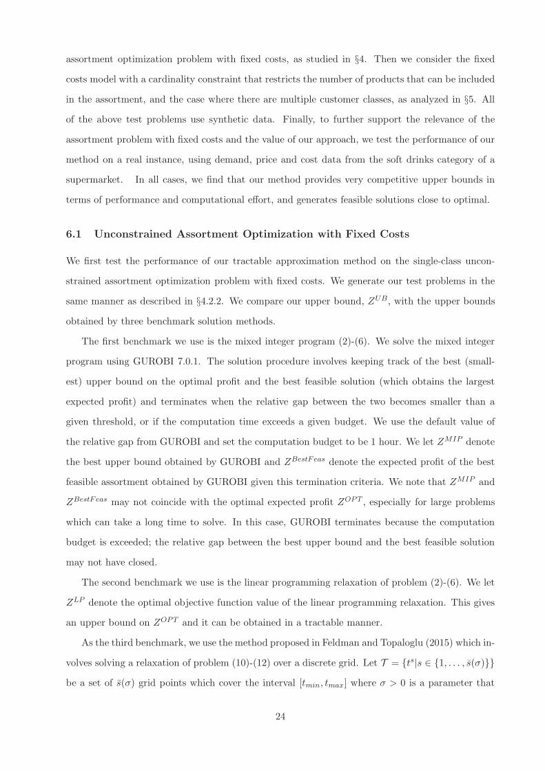
5 adds constraints and customer classes to the problem. Section 6 shows a numerical study of the

performance of our heuristic and Section 7 concludes. Proofs of the analytical results are included

in the Appendix.

2 Literature Review

We provide a concise review of the assortment planning literature under variants of the MNL choice

model. We refer the reader to Kok et al. (2009) for a more detailed review of the assortment planing

literature and Anderson et al. (1992) for a background on discrete choice models.

While there is a large and growing literature on assortment optimization under the MNL model

and variations of it, the majority of the works focus on the revenue maximization problem where

there are no product fixed costs. There is limited literature on the assortment problem with fixed

costs.

Kunnumkal et al. (2009) show that, under a MNL demand, the assortment optimization problem

with fixed costs is NP-hard. This is in contrast to the case without fixed costs, where the assortment

4

problem is known to be tractable under the MNL model (Talluri and van Ryzin 2004) and even

some variants of it (Davis et al. 2014). Kunnumkal et al. (2009) focus on approximation schemes

to obtain assortments with worst-case guarantees on the expected profit. The authors propose

a 2-approximation algorithm and a polynomial-time approximation scheme. The first algorithm

obtains an assortment which is guaranteed to obtain at least 50% of the optimal expected profit,

while the second one obtains assortments with improved guarantees but at the expense of increased

computational effort.

Feldman and Topaloglu (2015) consider the assortment optimization problem under the MMNL

model where there are no product fixed costs. Since the problem is intractable, they propose a

Lagrangian relaxation approach to obtain an upper bound on the optimal expected revenue. They

relax constraints that link the assortment decisions for the different customer classes by associating

Lagrange multipliers with them. Their relaxation involves solving an assortment problem with

product fixed costs for each segment where the Lagrange multipliers can be interpreted as fixed

costs. Since the fixed cost problem is intractable, they further propose a discrete grid-based ap-

proximation that obtains an upper bound on the optimal expected profit. While the primary focus

of Feldman and Topaloglu (2015) is the revenue optimization problem under the MMNL model,

their discrete grid-based approximation method can be used to obtain an upper bound for the

assortment problem with fixed costs. Subsequent to a working version of our paper, Kunnumkal

(2015) adapted our method to refine the Lagrangian relaxation approach of Feldman and Topaloglu

(2015) to the assortment problem under the MMNL model.

Schon (2010) considers the assortment pricing problem with fixed costs, where the decisions

are the prices to set for each product in the assortment. She proposes a convex mixed integer

programming (MIP) formulation to solve the problem exactly. Atamturk and Gomez (2017) propose

an approximation algorithm for maximizing a class of utility functions over a polytope. Their

method can be applied to the assortment problem with fixed costs provided the profit margins are

the same for all the products. Their method obtains a feasible solution and so provides a lower

bound on the optimal expected profit.

The papers closest to ours are Kunnumkal et al. (2009) and Feldman and Topaloglu (2015), but

there are some important differences. Kunnumkal et al. (2009) propose methods to obtain feasible

assortments with provable guarantees on the profits generated. The profits obtained by their

methods are lower bounds on the optimal expected profit. In contrast, we obtain an upper bound

on the optimal expected profit and our method does not necessarily yield a feasible solution since

5

there may be products included at fractional levels (although we can round it to obtain a feasible

solution with good performance; interestingly, this rounded solution is one of the solutions evaluated

in Kunnumkal et al. 2009). Our upper bound can therefore be used to better assess the optimality

gap of the candidate assortments obtained by Kunnumkal et al. (2009). For example, the 2-

approximation algorithm of Kunnumkal et al. (2009) obtains an assortment whose expected profit is

at least 50% of the optimal expected profit. This guarantee is from a worst-case perspective, can be

overly conservative and may not be very reassuring in practice. In our computational experiments,

we use our upper bound to verify that the assortments obtained by their 2-approximation algorithm

are in fact within a fraction of a percent of optimality. Our work therefore complements Kunnumkal

et al. (2009). Moreover, we extend our approach to handle general constraints on the assortment.

While the grid-based approximation method of Feldman and Topaloglu (2015) also obtains

an upper bound on the optimal expected profit, our method has certain appealing features. Our

upper bound is provably tighter than the grid-based approximation bound. The quality and the

computational work required to obtain the grid-based approximation bound depends on the density

of the grid, and there is a clear trade-off between the quality of the bound and the computation time.

Our method can be viewed as a version of the grid-based approximation of Feldman and Topaloglu

(2015) that works with an infinitely dense grid. However, the computational work required to

obtain our bound does not depend on the density of the grid and is instead polynomial in the

number of products. We also have theoretical guarantees on how far our upper bound can be from

the optimal expected profit.

Finally we note that there is a body of work on assortment planning with inventory costs; see for

example van Ryzin and Mahajan (1999). This line of work is primarily concerned with inventory

levels of the different products that balance the trade-off between stock-outs and inventory carrying

costs, and an underlying assumption is that customers make their choice without considering the

availability of the products. We do not rely on this assumption and in our model customers choose

after observing the assortment.

3 Problem Formulation

We have a set of n products and we have to decide which of them to include in the assortment.

We let J = {1, 2, . . . , n} denote the set of products and for product j ∈ J , we let pj denote its

profit margin and cj the fixed cost of including it in the assortment. We let xj ∈ {0, 1} indicate if

6

product j is included in the assortment. Given an assortment, customers choose among the offered

products according to the multinomial logit (MNL) model. The MNL model associates a preference

weight vj with product j and a preference weight v0 associated with not making a purchase. The

probability that a customer purchases product j is given by vjxj/(v0 +∑

k∈J vkxk) and the no-

purchase probability is given by v0/(v0 +∑

k∈J vkxk). We note that vj > 0 for all j and v0 ≥ 0;

however the preference weights are not necessarily integer valued. Normalizing the total market

size to 1 and letting

Z(x) =

∑

j∈J pjvjxj

v0 +∑

j∈J vjxj−∑

j∈Jcjxj (1)

denote the expected profit associated with offering the assortment x = {xj | ∀j}, the optimal ex-

pected profits can be obtained by solving the problem

(OPT ) ZOPT = max Z(x)

s.t. xj ∈ {0, 1}.

The optimal assortment can be obtained efficiently in certain special cases. For example, OPT is

tractable if the preference weights for all the products are identical, or if the no-purchase preference

weight v0 = 0. It is also tractable if the fixed costs are identical for all the products: cj = c for all

j. However, Kunnumkal et al. (2009) show that problem OPT is NP-hard in general. Furthermore,

Atamturk and Gomez (2017) show that the problem is intractable even when the profit contributions

are identical for all the products.

Although OPT is a nonlinear integer program, it can be reformulated as the linear mixed-integer

program

ZOPT = max∑

j∈Jpjuj −

∑

j∈Jcjxj (2)

s.t. v0vjuj ≤ u0 ∀j (3)

uj ≤ vjv0+vj

xj ∀j (4)

∑

j∈J uj + u0 = 1 (5)

uj ≥ 0, xj ∈ {0, 1} (6)

by using the transformation uj = vjxj/(v0+∑

k∈J vkxk); see for example Topaloglu (2013). While

the linear mixed-integer program is still intractable, it is in a form that can be readily handled by

7

most commercial optimization software. The mixed-integer programming formulation tends to be

more useful when we benchmark the performance of different approximation methods against the

optimal expected profit.

4 An Upper Bound Based on a Parametric Linear Program

In this section, we describe a tractable method to obtain an upper bound on the optimal expected

profit. If we let t = 1v0+

∑j∈J vjxj

, then Z(x) =∑

j∈J (pjvjt− cj)xj =∑

j∈J ρj(t)xj , where

ρj(t) = pjvjt− cj . (7)

Therefore, we can write OPT equivalently as

ZOPT = maxt∈[tmin,tmax]

Γb(t) (8)

where Vk =∑k

j=1 vj, tmin = 1Vn+v0

, tmax = 1minj{vj}+v0

and

Γb(t) = max∑

j∈Jρj(t)xj

s.t.∑

j∈J vjxj ≤ 1t − v0

xj ∈ {0, 1}.

Here we note that even though we have replaced the constraint∑

j∈J vjxj =1t−v0 with

∑

j∈J vjxj ≤1t − v0, the formulation remains valid since the constraint will be satisfied as an equality at a value

of t that maximizes Γb(t). Computing Γb(t) involves solving a binary knapsack problem, which is

again intractable (although they can be solved quickly with commercial solvers).

Since we are interested in obtaining a tractable upper bound on ZOPT , we consider the con-

tinuous relaxation of the binary knapsack. In doing so, we restrict our attention to the products

contained in the set

J (t) ={

j|vj ≤1

t− v0 and ρj(t) > 0

}

. (9)

This is because, if vj > 1t − v0, then product j can never be part of any feasible solution to the

binary knapsack. On the other hand, if ρj(t) ≤ 0, then product j can be excluded from an optimal

8

solution to the binary knapsack. Therefore, if j /∈ J (t) it cannot be part of an optimal solution to

the binary knapsack. Consequently, we can restrict attention to the products in J (t) when working

with the continuous relaxation of the binary knapsack

Γf (t) = max∑

j∈J (t)

ρj(t)xj (10)

s.t.∑

j∈J (t) vjxj ≤ 1t − v0 (11)

0 ≤ xj ≤ 1. (12)

Since Γb(t) ≤ Γf (t),

ZUB = maxt∈[tmin,tmax]

Γf (t) (13)

gives us an upper bound on the optimal expected profit.

Lemma 1. ZOPT ≤ ZUB.

While it is easy to see that ZUB is an upper bound on ZOPT , it is not immediately clear whether

the maximization in (13) can be carried out in a tractable manner. It is also not clear how well ZUB

approximates ZOPT . We explore these questions in the following sections. We note that Kunnumkal

et al. (2009) also use the parametric formulation Γb(t) of the assortment problem. However, as

mentioned, their focus is on obtaining candidate assortments with performance guarantees on the

expected profit.

4.1 Tractability

Problem (10)-(12) is a continuous knapsack problem and is tractable. However, its optimal solution

depends on the parameter t since the objective function coefficients and the knapsack size are

functions of t. Therefore, a potential difficulty in obtaining ZUB is that Γf (t) has to be computed

for infinitely many values of t. In this section, we show that it is sufficient to evaluate Γf (t) at a

finite, in fact a polynomial, number of values of t.

We begin with the observation that the optimal solution to a continuous knapsack problem

involves filling up the knapsack with items in decreasing order of the profit-to-space ratio until the

knapsack is completely filled. In the context of problem (10)-(12), we fill up the knapsack of size

1t − v0 with products in decreasing order of

ρj(t)vj

= pjt− cjvj.

9

Since the profit-to-space ratio depends on the value of t, the order in which the items get placed

into the knapsack also depends on the value of t. We bound the number of different orderings that

are possible as we vary t. Product k1 has a higher profit-to-space ratio than product k2 provided

(pk1 − pk2)t ≥ck1vk1

− ck2vk2

. Therefore, we have exactly one critical value tk1,k2 =ck1/vk1 − ck2/vk2

pk1 − pk2at

which the profit-to-space ordering of products k1 and k2 changes. Note that if tk1,k2 is smaller than

tmin or greater than tmax, then the profit-to-space ordering of k1 and k2 remains the same in the

entire range of t of interest. So we find the critical values tk1,k2 for every pair of products k1 and k2

and sort these O(n2) critical values from smallest to largest. This divides the interval [tmin, tmax]

into O(n2) subintervals. We note that the profit-to-space ordering of the products does not change

as t varies within a given subinterval. We conclude that there are O(n2) possible profit-to-space

orderings of the products.

Now consider a particular such subinterval [tl, tu]. For simplicity, assume that 1tu− v0 ≥ vmax =

maxj{vj} and that ρj(t) > 0 for all j, so that J (t) = J for all t ∈ [tl, tu]. Note that this is not a

restrictive assumption since if 1t − v0 < vmax, we simply work with a smaller set of products that

are admissible given the knapsack size 1t − v0. On the other hand, if ρj(t) ≤ 0 for some j, then we

can find the critical value of t at which the profit-to-space ratio of product j becomes equal to zero

and analyze the intervals to the left and right of the critical value separately.

Now suppose that ρ1(t)/v1 ≥ . . . ≥ ρn(t)/vn > 0 for all t ∈ [tl, tu]. Since (10)-(12) is a

continuous knapsack problem, we simply fill up the knapsack with products starting with product

1 until we use up all the space. Therefore,

Γf (t) =

κ(t)−1∑

j=1

ρj(t) + ρκ(t)(t)

(

1t − v0 − Vκ(t)−1

vκ(t)

)

where κ(t) is the largest index k such that Vk−1 =∑k−1

j=1 vj <1t −v0. Note that the index κ(t) stays

constant as long as Vk−1 < 1t − v0 ≤ Vk. Therefore, the interval [tl, tu] can be further partitioned

into O(n) subintervals such that κ(t) does not change with t within each subinterval. We note

that Kunnumkal et al. (2009) already make these observations in developing their approximation

algorithms. We build on them to next show that problem (13) can be solved in a tractable manner.

Since we have O(n2) intervals where the profit-to-space ordering of the products does not

change and each such interval can be further partitioned into O(n) subintervals where the index

κ(t) remains constant, the range [tmin, tmax] can be partitioned into a total of O(n3) subintervals

10

and problem (13) can be obtained by solving O(n3) problems of the form maxt∈[l,u]Πκ(t) where

Πκ(t) =

κ−1∑

j=1

ρj(t) + ρκ(t)

(

1t − v0 − Vκ−1

vκ

)

(14)

and Vκ−1 ≤ 1u − v0 and 1

l − v0 ≤ Vκ. Let

∆κ = pκ(v0 + Vκ−1)−κ−1∑

j=1

pjvj. (15)

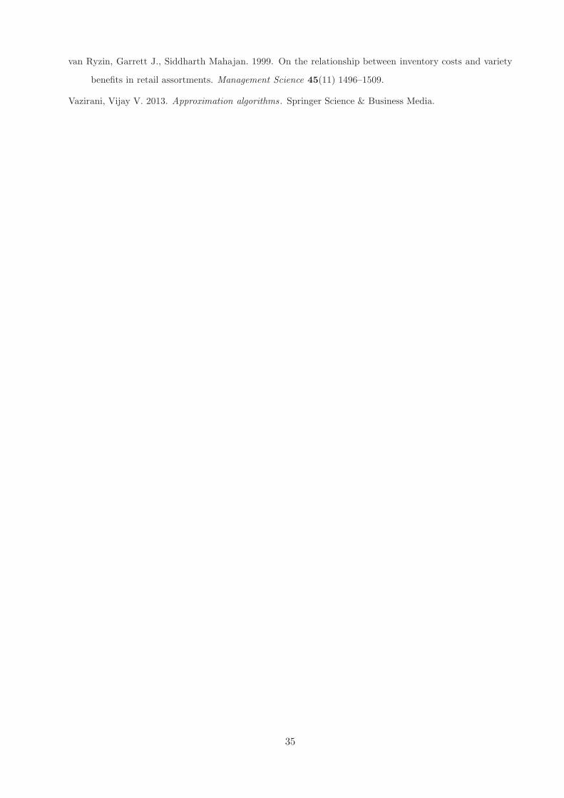
Lemma 2 below states that the problem maxt∈[l,u]Πκ(t) can be solved efficiently, essentially in

closed form.

Lemma 2. Let t∗ = argmaxt∈[l,u]Πκ(t). If ∆κ ≤ 0, then t∗ = u. Otherwise, t∗ = max {l,min {t∗, u}}

where

t∗ =

√

cκ/vκ∆κ

. (16)

We thus have the following proposition.

Proposition 1. ZUB can be obtained in a running time of O(n3).

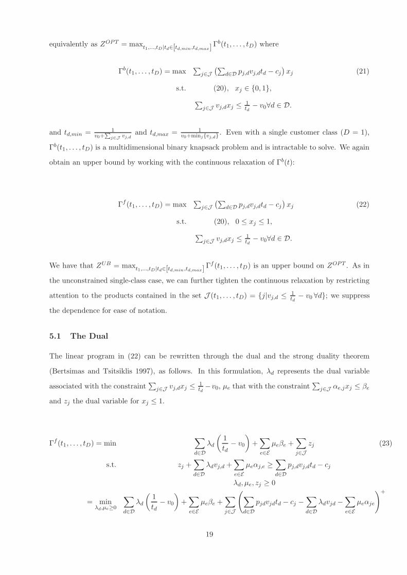
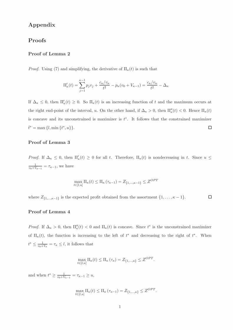
0.1 0.15 0.2 0.25 0.3

t

1.2

1.4

1.6

1.8

2

Pro

fit

Upper bound

Figure 1: Example with n = 3 products. Product characteristics are v0 = 1, v1 = 2, v2 =3, v3 = 4, p1 = 3.2, p2 = 2.8, p3 = 2, c1 = 0.4, c2 = 0.3, c3 = 0. The curve cor-responds to Γf (t), while the dots correspond to the integer solutions, i.e., all the points(

1v0+

∑3j=1 vjxj

,∑

3j=1

pjvjxj

v0+∑3

j=1 vjxj−∑3

j=1 cjxj

)

for xj ∈ {0, 1}.

To illustrate this result, we describe the intervals and sub-intervals in the following example,

see Figure 1. In the example, higher profit margins are associated with higher fixed costs but lower

11

levels of attractiveness (smaller preference weights). It turns out the optimal integer solution is

to introduce product 2 (with weight of 3), which results in a profit of 1.8. In contrast, the upper

bound is reached at t = 0.213 with a value of 1.8238, an optimality gap of 1.32% above the true

integer optimum.

To calculate the upper bound, we first compute t1,2 = 0.25, t1,3 = 0.166, t2,3 = 0.125. In

addition, we note that J (t) = {1, 2, 3} for t ≤ 0.2, J (t) = {1, 2} for t ∈ [0.2, 0.25] while J (t) = {1}

for t ∈ [0.25, 0.333]. This means, that, given that tmax = 1v0+v1

= 0.333 and tmin = 1v0+v1+v2+v3

=

0.1, we must consider five intervals [0.1, 0.125], [0.125, 0.166], [0.166, 0.2], [0.2, 0.25] and [0.25, 0.333]

in computing the upper bound.

1. In the first interval [0.1, 0.125], we have J (t) = {1, 2, 3} and ρ3(t)/v3 ≥ ρ2(t)/v2 ≥ ρ1(t)/v1.

In this interval, we have x3 = x2 = 1 and x1 varies between 1 and 0 and Γf (t) is increasing

in t.

2. In the second interval [0.125, 0.166], we still have J (t) = {1, 2, 3}, but ρ2(t)/v2 ≥ ρ3(t)/v3 ≥

ρ1(t)/v1. In this interval x2 = 1, x1 = 0 and x3 varies between 1 and 1/3 and Γf (t) is still

increasing in t.

3. In the third interval [0.166, 0.2] we have J (t) = {1, 2, 3} and ρ2(t)/v2 ≥ ρ1(t)/v1 ≥ ρ3(t)/v3.

In this interval x2 = 1, x3 = 0 and x1 varies from 1 to 0.5 and Γf (t) is increasing in t.

4. In the fourth interval [0.2, 0.25], the profit-to-space ordering of the products remains un-

changed but J (t) = {1, 2}. So we have x2 = 1 in this interval while x1 varies from 0.5 to 0.

Γf (t) is concave with an interior maximizer at 0.213 (as identified by Lemma 2).

5. Finally, in the last interval [0.25, 0.333], J (t) = {1}, which means that in this range the

optimal fractional solution stays equal to x1 = 1 and Γf (t) is increasing.

4.2 Performance Guarantees

In this section, we discuss the tightness of the upper bound ZUB. Kunnumkal et al. (2009) describe

an approximation algorithm which obtains an assortment whose expected profit is within a factor

of 2 of the optimal value. The same line of analysis here implies that ZUB ≤ 2ZOPT . We briefly

outline the arguments which show the performance bound of 2 and we give an example which shows

that the gap of 2 is in fact tight. On the other hand, in our computational experiments, we observe

that the gaps between ZUB and ZOPT tend to be much smaller than the theoretical worst-case

12

bound. To explain this, we characterize problem parameter settings where the gaps tend to be

small and provide improved performance guarantees in such cases.

4.2.1 A General Bound of 2

The analysis in Kunnumkal et al. (2009) implies that ZUB ≤ 2ZOPT . We summarize the key

observation for completeness. By (13) and (8), it suffices to show that Γf (t) ≤ 2Γb(t). But

this follows from the well-known result that the optimal objective function value of the fractional

knapsack is within a factor of 2 of that of the binary knapsack; see for example Vazirani (2013).

We next give an example where the gap between ZUB and ZOPT asymptotically approaches

2. We note that it is not a direct extension of the classical knapsack example, since in our setting

the objective function coefficients of the products and the knapsack size both depend on the same

underlying parameter t.

Consider an assortment problem with two products so that J = {1, 2}. Let v2 > v1 and

p2 > p1 > p2v2v0+v2

. Let c1 = v1(v0+v2)(v0+v1+v2)

[p1(v0 + v2) − p2v2] and c2 = v2v0+v1+v2

[p2 − p1v1v0+v1

], and

note that c1, c2 > 0. Since v2 > v1, tmin = 1v0+v1+v2

, tmax = 1v0+v1

and ZUB = maxt∈[tmin,tmax] Γf (t).

It can be verified that ρ1(t)/v1 ≥ ρ2(t)/v2 > 0 for all t ∈ [tmin, tmax]. Therefore when t = 1v0+v2

,

the knapsack includes product 1 and a fractional amount of product 2, so that

Γf

(

1

v0 + v2

)

= ρ1

(

1

v0 + v2

)

+ ρ2

(

1

v0 + v2

)(

v2 − v1v2

)

= Z{1} −p1v1(v2 − v1)

(v0 + v1)(v0 + v2)+

(

1− v1v2

)

Z{2},

where we use ZS to denote the expected profit associated with offering assortment S and the last

equality follows from using (7) and rearranging terms. Therefore Z{1} = ρ1

(

1v0+v1

)

denotes the

expected profit from offering the assortment consisting of product 1 alone, while Z{2} = ρ2

(

1v0+v2

)

denotes the expected profit from offering the assortment consisting of product 2 alone.

Now set v0 = 1, v1 = ǫ2, v2 = ǫ, p1 = 1/ǫ2 and p2 = 1/ǫ3, where 0 < ǫ < 1. It can be verified

that Z{1} and Z{2} tend to 1 as ǫ approaches 0 and the limit of ZOPT as ǫ approaches 0 is 1. Since

ZUB ≤ 2ZOPT , it follows that the limiting value of ZUB is no more than 2. On the other hand,

the limit of Γf(

1v0+v2

)

as ǫ approaches 0 is 2. Since ZUB = maxt∈[tmin,tmax] Γf (t) ≥ Γf ( 1

v0+v2), it

follows that the limiting value of ZUB as ǫ approaches 0 is 2. Therefore, the gap between ZUB and

ZOPT approaches 2 asymptotically.

13

4.2.2 Performance on Randomly Generated Instances

The example in §4.2.1 requires the preference weights and the profit margins of the products to

differ by orders of magnitude and this may not be the case in many situations, especially when we

think of the products as being substitutes of each other. So we investigate the performance of the

upper bound ZUB on randomly generated test problems.

We generate our test problems in a manner similar to Feldman and Topaloglu (2015). We have

n = 10 products. We set the preference weight of product j as vj = Xj/∑n

k=1Xk, where Xj is

uniformly distributed on [0, 1]. We set v0 = Φ1−Φ

∑

j∈J vj , where Φ ∈ [0, 1] is a parameter that

we vary in our computational experiments. Note that the no-purchase probability when all the

products are offered is Φ. We sample pj from the uniform distribution on [0, 2000] and sample cj

from the uniform distribution on [0, γpjvj/(v0 + vj)], where γ ∈ [0, 1] is a second parameter that

we vary in our computational experiments. We note that if γ is small, then the fixed costs are

relatively small compared to the profits. On the other hand, if γ is large, then the fixed costs are

roughly comparable to the profits. We vary Φ ∈ {0.75, 0.50, 0.25} and γ ∈ {1.00, 0.50, 0.25}. For

each (Φ, γ) combination, we generate 50 test problems by following the procedure described above.

Table 1 compares the upper bound ZUB with the optimal expected profit ZOPT , obtained by

solving its linear mixed-integer programming formulation (2)-(6). The first column of Table 1 gives

the problem parameters (n,Φ, µ). As mentioned, for each (Φ, γ) pair we generate 50 test problems

and the second column of Table 1 gives the average percentage difference (i.e., ZUB/ZOPT − 1)

over the 50 test problems. The third column gives the 5th percentile of the difference, while the

fourth column gives the 95th percentile. The last column reports the fraction of instances where

ZUB coincides with ZOPT .

We observe that ZUB is remarkably close to ZOPT in our computational experiments. The

average percentage difference is at most 0.58% and the 95th percentile of the difference is no more

than 3.49%. Moreover, ZUB coincides with ZOPT for at least half of the test problems, and

specifically the solution of problem (10)-(12) is integral, hence identifying the optimal solution. We

next provide a theoretical basis for these observations.

4.2.3 A Bound of 3/2

The example in §4.2.1 indicates that the gap between ZUB and ZOPT is essentially 2. On the

other hand, our computational experiments in §4.2.2 indicate that the performance of ZUB tends

to be much better than the worst-case bound of 2. In this section, we establish conditions for an

14

Problem % difference between ZUB and ZOPT % optimal(n,Φ, γ) Avg. 5th percentile 95th percentile

(10, 0.75, 1.00) 0.32 0.00 2.16 64(10, 0.75, 0.50) 0.16 0.00 0.54 72(10, 0.75, 0.25) 0.03 0.00 0.18 82(10, 0.5, 1.00) 0.34 0.00 1.71 60(10, 0.5, 0.50) 0.18 0.00 1.33 64(10, 0.5, 0.25) 0.10 0.00 0.59 66(10, 0.25, 1.00) 0.58 0.00 3.49 60(10, 0.25, 0.50) 0.16 0.00 1.07 66(10, 0.25, 0.25) 0.21 0.00 0.87 58

Table 1: Performance gap between ZUB and ZOPT for test problems with 10 products.

improved performance guarantee on the upper bound ZUB.

By the discussion in §4.1, it follows that ZUB can be obtained by solving O(n3) problems of the

form maxt∈[l,u]Πκ(t) where Vκ−1 =∑κ−1

j=1 vj ≤ 1u − v0 and 1

l − v0 ≤ Vκ =∑κ

j=1 vj . Equivalently,

u ≤ τκ−1 =1

v0+Vκ−1and l ≥ τκ = 1

v0+Vκ. So, to bound the gap between ZUB and ZOPT , it suffices

to obtain a uniform bound on the gap between maxt∈[l,u]Πκ(t) and ZOPT . In the following analysis,

we assume that 1u − v0 > vmax and J (t) = J for all t ∈ [l, u]. We emphasize that the assumptions

are only to reduce the notational burden and that all of our results continue to hold on relaxing

them.

Lemma 3. If ∆κ ≤ 0, then maxt∈[l,u]Πκ(t) ≤ ZOPT .

Lemma 4. Let t∗ = argmaxtΠκ(t). If ∆κ > 0 and t∗ ≥ τκ−1 or t∗ ≤ τκ, then maxt∈[l,u]Πκ(t) ≤

ZOPT .

Lemma 5. Let t∗ = argmaxtΠκ(t). If ∆κ > 0, t∗ ∈ (τκ, τκ−1) and t∗ ≤ 1v0+vκ

, then maxt∈[l,u]Πκ(t) ≤32Z

OPT .

Note that the only case not covered by Lemmas 3-5 is when ∆κ > 0 and 1v0+vκ

< t∗ < τκ−1.

That is, Vκ−1 < 1t∗ − v0 < vκ. We note that for this situation to occur the preference weight of

product κ has to be greater than the sum of the preference weights of products {1, . . . , κ−1}. This

is unlikely to be the case if the preference weights of the products are roughly similar and κ is

relatively large. That is, we are considering assortments that include a large number of products.

In the cases that are covered by Lemmas 3-5, the gap between ZUB and ZOPT is no more than

3/2. More interestingly, in the cases covered by Lemmas 3 and 4, we have ZOPT = ZUB and there

is no gap between the optimal expected profit and the upper bound. This explains to a certain

degree the good performance of ZUB that we observe in our computational experiments.

15

4.2.4 A Parametric Bound

The performance guarantees in §4.2.1 and §4.2.3 do not depend on the problem parameters. In this

section, we establish a bound that depends only on the preference weights of the products (and is

independent of the margins and product costs) and that can be potentially much tighter.

Recall that we can partition the interval [tmin, tmax] into O(n2) subintervals where the profit-

to-space ordering of the products do not change. Let [tl, tu] be such a subinterval and suppose that

we have ρ1(t)/v1 ≥ . . . ≥ ρn(t)/vn > 0 for all t ∈ [tl, tu]. Let κu be the largest index such that

tu ≤ τk = 1v0+Vk

and κl be the smallest index such that tl ≥ τk = 1v0+Vk

and note that κl > κu. So we

can write [tl, tu] = ∪κ∈{κl,...,κu+1}Iκ where Iκl= [tl, τκl−1] , Iκ = [τκ, τκ−1] for κ ∈ {κl−1, . . . , κu+2}

and Iκu+1 = [τκu+1, tu] and maxt∈[tl,tu] Γf (t) = maxκ∈{κl,...,κu+1}

{

maxt∈Iκ Πκ(t)}

. Therefore, in

order to bound the gap between ZUB = maxt∈[tmin,tmax] Γf (t) and ZOPT , it suffices to bound the

gap between maxt∈Iκ Πκ(t) and ZOPT : for κ ∈ {κl, . . . , κu + 1}, let

rκ = min

{

maxt∈Iκ Πκ(t)

Z{1,...,κ−1},maxt∈Iκ Πκ(t)

Z{1,...,κ}

}

− 1. (17)

Recall that Πκ(t) gives the expected profit for the assortment comprising of products {1, . . . , κ−1}

along with a fractional amount of product κ. Therefore, rκ can be interpreted as a measure of

the local optimality gap between the continuous relaxation and assortments obtained by “rounding

down” and “rounding up” the fractional product. Since ZOPT ≥ max{Z{1,...,κ−1}, Z{1,...,κ}}, rκ is

thus an upper bound on the relative gap between maxt∈Iκ Πκ(t) and ZOPT .

In the remainder of this section, we establish a bound on rκ when κ ∈ {κl − 1, . . . , κu+2}. The

analysis can be adapted to the cases when κ ∈ {κl, κu + 1}; we defer the details to the Appendix.

We let κ ∈ {κl − 1, . . . , κu + 2} and consider different scenarios.

First, if ∆κ ≤ 0, then Πκ(t) is decreasing (Lemma 2) hence maxt∈Iκ Πκ(t) = Πκ (τκ−1) =

Z{1,...,κ−1} and rκ = 0. Otherwise, ∆κ > 0 and hence Πκ(t) is concave; let t∗ denote the uncon-

strained maximizer of Πκ(t) (Lemma 2). If t∗ ≥ τκ−1, then maxt∈Iκ Πκ(t) = Πκ (τκ−1) = Z{1,...,κ−1}

and rκ = 0. Similarly, if t∗ ≤ τκ, then maxt∈Iκ Πκ(t) = Πκ (τκ) = Z{1,...,κ} and again rκ = 0.

The three cases considered so far result in a trivial bound on rκ. To obtain a non-trivial bound,

we consider the last case where ∆κ > 0 and t∗ ∈ [τκ, τκ−1], so that maxt∈Iκ Πκ(t) = Πκ(t∗). Lemma

6 below shows that rκ is maximal when the assortments {1, . . . , κ− 1} and {1, . . . , κ} generate the

same expected profits.

Lemma 6. Let κ ∈ {κl − 1, . . . , κu + 2}. If ∆κ > 0 and t∗ ∈ [τκ, τκ−1], then rκ is maximal when

16

Z{1,...,κ−1} = Z{1,...,κ}.

Since we are interested in obtaining an upper bound on the gap between ZOPT and maxt∈Iκ Πκ(t) =

Πκ(t∗), we restrict ourselves to the case where rκ is maximal: Z{1,...,κ−1} = Z{1,...,κ} implies

cκvκ

=∆κ

(v0 + Vκ−1)(v0 + Vκ). (18)

which yields after some algebra - see Equation (31) in the Appendix:

rκ =∆κ

(√v0 + Vκ −

√v0 + Vκ−1

)2

(v0 + Vκ−1)(v0 + Vκ)Z{1,...,κ−1}. (19)

Lemma 7 below gives a lower bound on Z{1,...,κ−1} which we use, in turn, to bound rκ.

Lemma 7. Let κ ∈ {κl − 1, . . . , κu + 2}. If ∆κ > 0 and t∗ ∈ [τκ, τκ−1], then Z{1,...,κ−1} ≥∆κVκ−1

v0(v0+Vκ−1)

(

1−√

v0+Vκ−1

v0+Vκ

)

.

Using the lower bound from Lemma 7 in Equation (19), we obtain the following proposition.

Proposition 2. Let κ ∈ {κl − 1, . . . , κu + 2}. If ∆κ > 0 and t∗ ∈ [τκ, τκ−1], then

rκ ≤ v0vκ

Vκ−1

√v0 + Vκ(

√v0 + Vκ +

√v0 + Vκ−1)

.

Proposition 2 together with the observations preceding Lemma 6 provide a complete charac-

terization of the performance gap for the intervals Iκ with κ ∈ {κl − 1, . . . , κu + 2}: if ∆κ > 0

and t∗ ∈ [τκ, τκ−1], then the bound in Proposition 2 applies, otherwise rκ = 0. As mentioned, it

is possible to adapt the analysis to obtain similar bounds for the intervals Iκland Iκu+1; we defer

the details to the Appendix.

Applying the parametric bound to the example in Figure 1, we obtain a bound of 23√6(√6+

√3)

=

6.51%. This follows from using Proposition 2 to the interval where product 2 is fully included and

the marginal product is 1: v0 = 1, vκ = 2, Vκ−1 = 3.

We note that the numerator of the bound in Proposition 2 depends on the preference weight

of product κ, while the denominator is a function of the sum of the preference weights of products

{1, . . . , κ− 1}, Vκ−1, and the sum of the preference weights of products {1, . . . , κ}, Vκ. The bound

becomes large when vκ is much larger than Vκ−1 and its worst case value is not better than 2. On

17

the other hand, if the preference weights of the products are not dramatically different and we are

considering assortments with a relatively large number of products, then we expect the denominator

of the upper bounding term to dominate the numerator and rκ to be quite small. In such cases, we

expect ZUB to be quite close to ZOPT as well. The parametric bound thus provides more insight

into why the gap between ZUB and ZOPT is often small in our computational experiments.

5 Assortment Planning with Fixed Costs, Constraints and Multi-

ple Classes

In this section, we consider the assortment problem with fixed costs with additional constraints

on the assortment and multiple customer classes, i.e., mixture of logit demands. To solve this

more complex problem, we provide a dual formulation for our upper bound. We then study the

tractability of the solution method and discuss its performance guarantees.

We now add a total of E constraints that limit the assortments that can be offered:

∑

j∈Jαe,jxj ≤ βe ∀e ∈ E (20)

where E = {1, . . . , E} denotes the set of constraints.

We also consider multiple customer classes d ∈ D = {1, . . . ,D} and let θd denote the fraction

of customers belonging to class d so that∑

d∈D θd = 1. We let vj,d denote the preference weight

associated with class d for product j (we keep v0,d = v0 without loss of generality) and pj,d its

corresponding margin. Let Z(x) =∑

d∈D θd

∑j∈J pj,dvj,dxj

v0+∑

j∈J vj,dxj−∑j∈J cjxj =

∑

d∈D

∑j∈J pj,dvj,dxj

v0+∑

j∈J vj,dxj−

∑

j∈J cjxj, where pj,d = θdpj,d can be interpreted as the expected margin for product j from class

d. The optimal expected profits for this extension can be obtained by solving

(OPT ) ZOPT = max Z(x)

s.t. (20), xj ∈ {0, 1}.

Note that this formulation is generic enough to allow for the same product to be sold at different

prices to different customer classes. This may be useful in situations where the different classes are

mapped to different retail stores and there is flexibility in terms of setting the store prices.

As in the unconstrained case, we can write the constrained assortment optimization problem

18

equivalently as ZOPT = maxt1,...,tD |td∈[td,min,td,max] Γb(t1, . . . , tD) where

Γb(t1, . . . , tD) = max∑

j∈J(∑

d∈D pj,dvj,dtd − cj)

xj (21)

s.t. (20), xj ∈ {0, 1},∑

j∈J vj,dxj ≤ 1td

− v0∀d ∈ D.

and td,min = 1v0+

∑j∈J vj,d

and td,max = 1v0+minj{vj,d} . Even with a single customer class (D = 1),

Γb(t1, . . . , tD) is a multidimensional binary knapsack problem and is intractable to solve. We again

obtain an upper bound by working with the continuous relaxation of Γb(t):

Γf (t1, . . . , tD) = max∑

j∈J(∑

d∈D pj,dvj,dtd − cj)

xj (22)

s.t. (20), 0 ≤ xj ≤ 1,

∑

j∈J vj,dxj ≤ 1td

− v0∀d ∈ D.

We have that ZUB = maxt1,...,tD |td∈[td,min,td,max] Γf (t1, . . . , tD) is an upper bound on ZOPT . As in

the unconstrained single-class case, we can further tighten the continuous relaxation by restricting

attention to the products contained in the set J (t1, . . . , tD) = {j|vj,d ≤ 1td

− v0 ∀d}; we suppress

the dependence for ease of notation.

5.1 The Dual

The linear program in (22) can be rewritten through the dual and the strong duality theorem

(Bertsimas and Tsitsiklis 1997), as follows. In this formulation, λd represents the dual variable

associated with the constraint∑

j∈J vj,dxj ≤ 1td−v0, µe that with the constraint

∑

j∈J αe,jxj ≤ βe

and zj the dual variable for xj ≤ 1.

Γf (t1, . . . , tD) = min∑

d∈Dλd

(

1

td− v0

)

+∑

e∈Eµeβe +

∑

j∈Jzj (23)

s.t. zj +∑

d∈Dλdvj,d +

∑

e∈Eµeαj,e ≥

∑

d∈Dpj,dvj,dtd − cj

λd, µe, zj ≥ 0

= minλd,µe≥0

∑

d∈Dλd

(

1

td− v0

)

+∑

e∈Eµeβe +

∑

j∈J

(

∑

d∈Dpjdvjdtd − cj −

∑

d∈Dλdvjd −

∑

e∈Eµeαje

)+

19

where x+ = max{x, 0}. As we can see, this dual formulation only requires the optimization of a

piecewise-linear objective over λd, µe ≥ 0. This suggests that, given (t1, . . . , tD), the upper bound

can be computed quickly, by inspecting all the break-points of the piecewise-linear function.

5.2 Alternative View of the Single-class, Unconstrained Case

When we have a single class and no constraints (D = 1, E = 0), then we recover the continuous

knapsack problem described in §3: indeed the minimum of (23) is reached at λ equal to 0 or

[ρj(t)/vj ]+ = [pjt−cj/vj ]

+ for some j, where we drop the customer class index d from the subscripts

to simplify the notation. Assuming without loss of generality (as before in §4.1) that ρ1(t)/v1 ≥

. . . ≥ ρn(t)/vn ≥ 0, then the primal solution associated with λ = ρκ(t)/vκ is to select xj = 1 for

j ≤ κ− 1, a fractional value for xκ, and xj = 0 for j > κ, which results in an objective equal to

Gκ(t) =

κ−1∑

j=1

ρj(t)vj +ρκ(t)

vκ

1

t− v0 −

κ−1∑

j=1

vj

.

We define for completeness νn+1(t) = 0 so Gn+1(t) =∑

j∈J (ρj(t)vj − cj) and

Γf (t) = minκ∈J

Gκ(t). (24)

As a result, if we now want to maximize this value by changing t (within the interval such that

the order of ρj(t)/vj does not change), then the maximum over t can be either interior, i.e., there

is κ such that t∗ = argmax Gκ(t), in which case it is the same value identified in Lemma 2;

or at a breakpoint t such that Gκ(t) = Gκ+1(t). This is a quadratic equation in t, with roots

(pκ − pκ+1)t =cκvκ

− cκ+1

vκ+1, i.e., t = tκ,κ+1, and t = 1

v0+Vκ. We thus recover all the results presented

in §4.1.

5.3 General Case

In the general case with assortment constraints and multiple customer classes, the problem in (23)

is a minimization of a piecewise-linear function of {λd|∀d ∈ D} and {µe|∀e ∈ E}. Compared to

§5.2, instead of a search over one dimension (that of λ), we must now search a space of D + E

dimensions, so the number of breakpoints to consider for each (t1, . . . , tD) isn!

(D+E)!(n−D−E)! , thus

O(nD+E), polynomial in n but exponential in D +E. Still the structure conceptually remains the

same as the single-class unconstrained case. Lemma 8 below is the analog of Equation (24) in the

20

unconstrained case.

Lemma 8. Γf (t1, . . . , tD) is the minimum of O(nD+E) functions of the form

Gκ(t1, . . . , tD) =∑

d1,d2∈Dηκ,d1,d2

td1td2

+∑

d∈Dξκ,dtd +

∑

d∈Dχκ,d

1

td+ φκ, (25)

for appropriately defined ηκ,d1,d2 , ξκ,d, χκ,d, φκ.

Hence, in the general case, we find that Γf (·) can still be computed relatively easily for a given

(t1, . . . , tD). However, the existence of multiple classes complicates the functional shape of Gκ(·),

which are fractional functions of (t1, . . . , tD). The coefficients of Gκ(·), ηκ,d1,d2 , ξκ,d, χκ,d and φκ are

specified in the proof of the lemma and are more complex to compute since they require the inversion

of a square matrix of dimension D + E. This can be done in a complexity of O(

max(D,E)3)

, by

Gauss-Jordan elimination for example.

To generate the upper bound ZUB, we must now search for values of (t1, . . . , tD) that maximize

Γf (·). This is an easy task when there is a single class.

Lemma 9. When D = 1, Γf (t) is either maximized at:

1. t∗κ =√

χκ

ξκ(when the term inside the square root is positive);

2. or, tκ1,κ2one of the two solutions of

ηκ1+ φκ1

+ ξκ1t+ χκ1

1

t= ηκ2

+ φκ2+ ξκ2

t+ χκ2

1

t.

Hence, under a single customer class, it is sufficient to inspect a polynomial number of values of

t. The number to inspect is dominated by the number of tκ1κ2: O(n2+2E), the order of the square

of the number of functions Gκ(t) that we consider. For each of these values of t, we then need to

compare the O(n1+E) values of Gκ(t). Taking into account that matrix inversion in this case takes

O(E3), we thus have the following proposition.

Proposition 3. When D = 1, ZUB can be obtained in a running time of O(E3n1+E + n3+3E).

This extends Proposition 1 by incorporating assortment constraints. In the constrained case, we

obtain a pseudo-polynomial complexity. Given that typically the number of products is very large

but the number of constraints small (constraints on the total number of products and/or space

consumed by the products), this means that our method will run reasonably fast in an application.

21

When we have multiple classes, the problem becomes more complicated. Indeed, the maximizer

of Γf (t1, . . . , tD) can be of two kinds. One possibility is that it is the minimizer of a given Gκ, in

which case we need to first characterize such a minimizer (as in the first case of Lemma 9), and

then to guarantee that there is a polynomial number of those. The other possibility is that the

solution happens to be at a (t1, . . . , tD) such that multiple Gκ attain the same value (although

it is not a local minimum for any of the Gκ), in which case we need to solve equations such as

those in the second case of Lemma 9. There are some special cases where the problem is tractable

(when preference weights are identical across classes), but in general we need to resort to numerical

optimization methods when D ≥ 2.

5.4 Primal Solutions and Performance Guarantees

The dual approach outlined above provides a way of computing ZUB. However, it is not a priori

clear that we can generate primal solutions easily. In the unconstrained case, the upper bound was

associated with a fractional solution xj such that at most one product had a non-integer value. We

found that including or excluding this item in the assortment provided a solution with a guaranteed

performance (see §4.2). When there are multiple products with non-integer values, then one must

consider including or excluding any of them, and there may potentially an exponential number

of such combinations. This has two implications. First, there is no direct way to obtain a good

solution from the tractable computation of the upper bound. Second, we may not be able to

guarantee the performance of such a heuristic, as we did before.

Fortunately, we identify in this section some common cases where the “rounding” process can be

done in a simple way, without degrading the performance guarantee obtained for the unconstrained

case. Throughout we assume D = 1, t ≤ 1v0+max{vj} and J (t) = J .

5.4.1 Cardinality Constraints

Consider that we have a constraint on the size of the assortment, so that the total number of items

offered is no more than K:∑

j∈J xj ≤ K, where K ≥ 1. Cardinality constraints arise when there

is a need to limit the total number of products in the assortment for operational reasons; see e.g.,

Rusmevichientong et al. (2010), Gallego and Topaloglu (2014).

We show that Γf (t) ≤ 2Γb(t) when we have a cardinality constraint. The proof follows by

noting that an optimal solution to Γf (t) has at most two variables that assume fractional values.

By carefully rounding the fractional values, we obtain two integer solutions that are each feasible

22

to the binary knapsack problem; we defer the details to the Appendix. Using the two feasible

solutions we show that Γf (t) ≤ 2Γb(t). This implies the following result.

Proposition 4. For the assortment problem with fixed costs and a cardinality constraint, we have

ZUB ≤ 2ZOPT .

We note that the bound can be extended to the case with nested cardinality constraints. That

is, we have nested subsets of products S1 ⊂ . . . ⊂ Sm with cardinality restrictions K1 ≤ . . . ≤ Km,

respectively. The arguments also apply to the case where the products are partitioned into disjoint

subsets with associated restrictions on the cardinality of each subset; see Davis et al. (2013).

5.4.2 Product Precedence Constraints

Consider now that we have constraints which link the offer decisions for the different products. In

particular, associated with each product j, we have a subset Oj of products that have to be offered

if product j is offered. That is, we have xj − xi ≤ 0 for all i ∈ Oj . We follow the convention

that j ∈ Oj . We consider the case where the precedence constraints are nested in the following

sense: for two products j and k, we either have Oj ⊂ Ok or Ok ⊂ Oj or Oj ∩ Ok = ∅. Product

precedence constraints may arise in situations where say a more expensive variant or style cannot

be included in the assortment unless a basic version of the product is also part of the assortment;

see for example Davis et al. (2013).

We show that Γf (t) ≤ 2Γb(t) when we have nested product precedence constraints. The proof

follows from the observation that an optimal solution to Γf (t) has at most one distinct fractional

value. Moreover all the variables assuming this fractional value are contained in Oj for some

product j. By carefully rounding the fractional valued variables, we obtain two integer solutions

that are each feasible to the binary knapsack problem; we defer the details to the Appendix. We

stitch together the two feasible solutions to show that Γf (t) ≤ 2Γb(t), which in turn implies the

following result.

Proposition 5. For the assortment problem with fixed costs and nested product precedence con-

straints, we have ZUB ≤ 2ZOPT .

6 Computational Experiments

We now compare the performance of our tractable approximation method with that of benchmark

solution methods, on different test problems. We first consider the single-class unconstrained

23

assortment optimization problem with fixed costs, as studied in §4. Then we consider the fixed

costs model with a cardinality constraint that restricts the number of products that can be included

in the assortment, and the case where there are multiple customer classes, as analyzed in §5. All

of the above test problems use synthetic data. Finally, to further support the relevance of the

assortment problem with fixed costs and the value of our approach, we test the performance of our

method on a real instance, using demand, price and cost data from the soft drinks category of a

supermarket. In all cases, we find that our method provides very competitive upper bounds in

terms of performance and computational effort, and generates feasible solutions close to optimal.

6.1 Unconstrained Assortment Optimization with Fixed Costs

We first test the performance of our tractable approximation method on the single-class uncon-

strained assortment optimization problem with fixed costs. We generate our test problems in the

same manner as described in §4.2.2. We compare our upper bound, ZUB, with the upper bounds

obtained by three benchmark solution methods.

The first benchmark we use is the mixed integer program (2)-(6). We solve the mixed integer

program using GUROBI 7.0.1. The solution procedure involves keeping track of the best (small-

est) upper bound on the optimal profit and the best feasible solution (which obtains the largest

expected profit) and terminates when the relative gap between the two becomes smaller than a

given threshold, or if the computation time exceeds a given budget. We use the default value of

the relative gap from GUROBI and set the computation budget to be 1 hour. We let ZMIP denote

the best upper bound obtained by GUROBI and ZBestFeas denote the expected profit of the best

feasible assortment obtained by GUROBI given this termination criteria. We note that ZMIP and

ZBestFeas may not coincide with the optimal expected profit ZOPT , especially for large problems

which can take a long time to solve. In this case, GUROBI terminates because the computation

budget is exceeded; the relative gap between the best upper bound and the best feasible solution

may not have closed.

The second benchmark we use is the linear programming relaxation of problem (2)-(6). We let

ZLP denote the optimal objective function value of the linear programming relaxation. This gives

an upper bound on ZOPT and it can be obtained in a tractable manner.

As the third benchmark, we use the method proposed in Feldman and Topaloglu (2015) which in-

volves solving a relaxation of problem (10)-(12) over a discrete grid. Let T = {ts|s ∈ {1, . . . , s(σ)}}

be a set of s(σ) grid points which cover the interval [tmin, tmax] where σ > 0 is a parameter that

24

controls the size of the grid. Feldman and Topaloglu (2015) propose using an exponential grid so

that ts = (1+σ)ts−1. As σ becomes smaller, the spacing between the grid points decreases and we

obtain denser grids. Further, Feldman and Topaloglu (2015) propose solving a relaxation of prob-

lem (10)-(12) over the intervals defined by the grid points and take the maximum of these values

to obtain an upper bound on the optimal expected profit. We denote the upper bound obtained

by this method as ZDG(σ) where the argument emphasizes the dependence of the solution on the

density of the grid. In our computational experiments, we consider three different grid densities by

varying σ over the set {0.1, 0.01, 0.001}. Note that the grids get progressively denser as σ varies

from 0.1 to 0.001.

It is possible to show that ZUB is provably tighter than ZLP and ZDG(σ) for all σ > 0. In

our computational experiments we study the relative tightness of the upper bounds and how much

ZUB improves upon ZLP and ZDG(σ).

Table 2 shows the tightness of the upper bounds obtained by the different solution methods for

assortment problems with n = 100 products. The first column describes the problem characteristics

using (n,Φ, γ). For each parameter combination, we generate 50 test problems in the manner

described in §4.2.2. The second column of the table gives the average percentage difference between

ZUB and ZBestFeas. We note that this gap is an upper bound on the gap between ZUB and ZOPT

since the profit of the best feasible solution is no larger than ZOPT . The third column gives

the 95th percentile of the difference between ZUB and ZBestFeas. The fourth column reports

the value of the parametric bound described in §4.2.4 averaged over the 50 problem instances.

The remaining columns report the averages and the 95th percentiles of the gaps of ZMIP , ZLP ,

ZDG(0.1), ZDG(0.01) and ZDG(0.001) relative to ZBestFeas, respectively.

% difference with best feas. soln. from MIP

ZUB ZMIP ZLP ZDG(0.1) ZDG(0.01) ZDG(0.001)Problem Avg. 95% Param. Avg. 95% Avg. 95% Avg. 95% Avg. 95% Avg. 95%(n,Φ, γ) bound

(100, 0.75, 1.00) 0.01 0.06 0.60 0.00 0.01 27 42 15 18 1.53 1.79 0.16 0.19(100, 0.75, 0.50) 0.00 0.02 0.36 0.50 4.25 27 41 14 16 1.41 1.61 0.14 0.17(100, 0.75, 0.25) 0.00 0.03 0.23 0.00 0.01 16 26 12 13 1.24 1.30 0.13 0.14(100, 0.50, 1.00) 0.03 0.11 0.60 0.00 0.01 34 46 14 16 1.44 1.67 0.17 0.26(100, 0.50, 0.50) 0.01 0.02 0.65 0.31 2.78 29 41 13 15 1.34 1.50 0.14 0.16(100, 0.50, 0.25) 0.00 0.01 0.44 0.00 0.01 20 29 12 13 1.23 1.33 0.13 0.14(100, 0.25, 1.00) 0.02 0.09 1.73 0.00 0.00 35 47 14 16 1.36 1.56 0.15 0.22(100, 0.25, 0.50) 0.02 0.02 0.98 0.00 0.00 31 45 13 14 1.29 1.45 0.14 0.16(100, 0.25, 0.25) 0.01 0.06 0.65 0.00 0.01 24 38 12 13 1.23 1.32 0.14 0.18

Table 2: Comparison of upper bounds for assortment problems with n = 100 products.

We note that when the percentage difference between ZMIP and ZBestFeas is zero, it means that

25

GUROBI is able to solve the mixed integer program (2)-(6) within the given time limit and we have

ZMIP = ZBestFeas = ZOPT . One interesting observation is that this does not always happen: there

are test problems where the mixed integer program cannot be solved to optimality within 1 hour

and the gap between ZMIP and ZBestFeas can be as much as 4%. The percentage difference between

ZUB and ZBestFeas is around 0.02% on average. Since ZUB is an upper bound on the optimal profit

and ZBestFeas is a lower bound, we conclude that ZUB and ZBestFeas are near-optimal. Therefore,

the gap in the mixed integer program arises from the upper bound ZMIP being relatively loose.

The parametric bound of §4.2.4 gives a more accurate picture of the performance of ZUB compared

to the constant factor bounds of 2 and 3/2 (which would imply percentage differences of 100%

and 50%, respectively). This is in line with Proposition 2 which indicates that the gap between

ZUB and ZOPT is likely to be small for assortments including a large number of products. To our

knowledge, similar theoretical guarantees are not available for the other methods to obtain upper

bounds. The performance of the LP relaxation tends to be quite poor in comparison and the gaps

are around 25% on average. The quality of the upper bound obtained by the grid-based method,

ZDG(σ), improves as σ becomes smaller. ZDG(0.1) is somewhat loose, ZDG(0.01) is tighter and

ZDG(0.001) is quite close to ZUB.

Table 3 gives the CPU seconds required to obtain the different upper bounds for the test

problems with n = 100 products. We report both the average times as well as the maximum times

across the 50 instances for each parameter combination. All of our computational experiments are

carried out on a Core i7 desktop with 3.4-GHz CPU and 16-GB RAM. We use GUROBI 7.0.1

to solve all linear and mixed integer programs. ZLP and ZDG(0.1) can be obtained in less than

1/100 of a second. ZUB, ZDG(0.01) and ZDG(0.001) take slightly longer but all the upper bounds

can be obtained in a fraction of a second. The solution time of the grid-based method increases

as σ becomes smaller (and thus the number of grid points becomes larger). In contrast, the time

required to solve the mixed integer program is much longer and we observe instances where the

problem cannot be solved to optimality even after 1 hour. This is not surprising given that the

assortment optimization problem with fixed costs is an NP-hard problem. On the other hand, ZUB

can still be obtained in a fraction of a second.

Tables 4 and 5 give the different upper bounds and their computation times for the test problems

with n = 200 products. We observe that GUROBI is unable to solve the mixed integer program

even after 1 hour in many cases. The gap between the best upper bound it finds ZMIP and the

profit of the best feasible solution ZBestFeas can be as much as 16%. On the other hand, the gap

26

Problem CPU secs.ZUB ZMIP ZLP ZDG(0.1) ZDG(0.01) ZDG(0.001)

(n,Φ, γ) Avg. Max Avg. Max Avg. Max Avg. Max Avg. Max Avg. Max

(100, 0.75, 1.00) 0.04 0.08 6 95 0.00 0.02 0.00 0.01 0.00 0.01 0.02 0.05(100, 0.75, 0.50) 0.05 0.09 676 3600 0.01 0.02 0.00 0.00 0.00 0.01 0.02 0.09(100, 0.75, 0.25) 0.03 0.09 97 2211 0.01 0.01 0.00 0.00 0.00 0.01 0.02 0.06(100, 0.50, 1.00) 0.06 0.09 4 52 0.01 0.01 0.00 0.01 0.00 0.01 0.03 0.10(100, 0.50, 0.50) 0.06 0.09 701 3600 0.01 0.01 0.00 0.00 0.00 0.01 0.03 0.08(100, 0.50, 0.25) 0.05 0.11 42 661 0.01 0.01 0.00 0.00 0.00 0.01 0.03 0.09(100, 0.25, 1.00) 0.06 0.08 1 9 0.01 0.01 0.00 0.00 0.00 0.01 0.04 0.06(100, 0.25, 0.50) 0.07 0.09 7 23 0.01 0.01 0.00 0.00 0.00 0.01 0.04 0.07(100, 0.25, 0.25) 0.06 0.11 57 2192 0.01 0.01 0.00 0.00 0.00 0.01 0.04 0.08

Table 3: CPU seconds to obtain the different upper bounds for assortment problems with n = 100products.

between ZUB and ZBestFeas is essentially zero in almost all cases. Therefore, ZUB and ZBestFeas

coincide with ZOPT . Taken together, this means that while GUROBI is able to find the optimal

assortment, it does not terminate because the upper bound it obtains is weak. On the other hand,

ZUB is near optimal and can be computed in a fraction of a second.

% difference with best feas. soln. from MIP

ZUB ZMIP ZLP ZDG(0.1) ZDG(0.01) ZDG(0.001)Problem Avg. 95% Param. Avg. 95% Avg. 95% Avg. 95% Avg. 95% Avg. 95%(n,Φ, γ) bound

(200, 0.75, 1.00) 0.00 0.01 0.62 2.80 8.94 28 44 15 17 1.49 1.72 0.15 0.17(200, 0.75, 0.50) 0.00 0.01 0.18 7.28 14.42 26 38 14 15 1.40 1.53 0.14 0.15(200, 0.75, 0.25) 0.00 0.01 0.13 4.28 10.98 16 33 12 13 1.24 1.33 0.12 0.13(200, 0.50, 1.00) 0.00 0.01 0.55 3.87 9.32 31 39 14 17 1.41 1.66 0.14 0.17(200, 0.50, 0.50) 0.00 0.02 0.30 8.55 16.80 29 36 13 15 1.32 1.50 0.13 0.15(200, 0.50, 0.25) 0.00 0.01 0.20 6.53 12.48 22 32 13 13 1.26 1.33 0.13 0.13(200, 0.25, 1.00) 0.01 0.05 0.69 1.21 7.24 32 44 13 15 1.31 1.47 0.14 0.17(200, 0.25, 0.50) 0.00 0.02 0.51 7.09 15.64 31 39 13 14 1.27 1.38 0.13 0.15(200, 0.25, 0.25) 0.00 0.01 0.45 8.22 12.60 25 31 12 13 1.24 1.32 0.13 0.14

Table 4: Comparison of upper bounds for assortment problems with n = 200 products.

Problem CPU secs.ZUB ZMIP ZLP ZDG(0.1) ZDG(0.01) ZDG(0.001)

(n,Φ, γ) Avg. Max Avg. Max Avg. Max Avg. Max Avg. Max Avg. Max

(200, 0.75, 1.00) 0.24 0.39 2326 3600 0.02 0.03 0.00 0.02 0.00 0.01 0.03 0.12(200, 0.75, 0.50) 0.24 0.47 2838 3600 0.02 0.06 0.00 0.00 0.00 0.01 0.03 0.09(200, 0.75, 0.25) 0.17 0.50 2303 3600 0.03 0.05 0.00 0.00 0.00 0.01 0.03 0.10(200, 0.50, 1.00) 0.27 0.35 2270 3600 0.02 0.03 0.00 0.00 0.00 0.01 0.04 0.09(200, 0.50, 0.50) 0.36 0.50 2651 3600 0.02 0.03 0.00 0.00 0.01 0.01 0.04 0.11(200, 0.50, 0.25) 0.26 0.53 3207 3600 0.02 0.03 0.00 0.00 0.00 0.01 0.04 0.11(200, 0.25, 1.00) 0.30 0.38 1125 3600 0.01 0.02 0.00 0.01 0.01 0.01 0.05 0.10(200, 0.25, 0.50) 0.40 0.47 2509 3600 0.01 0.03 0.00 0.00 0.01 0.01 0.05 0.11(200, 0.25, 0.25) 0.36 0.53 3148 3600 0.02 0.03 0.00 0.00 0.01 0.01 0.05 0.12

Table 5: CPU seconds to obtain the different upper bounds for assortment problems with n = 200products.

Feldman and Topaloglu (2015) show that if the fixed costs satisfy a particular scaling property,

27

then no grid, no matter how dense, can improve upon ZDG(σ) by more than a factor of (1 + σ).

However, if the fixed costs do not satisfy the scaling property, then the performance guarantee in

Feldman and Topaloglu (2015) does not hold. In our test problems the product fixed costs do not

scale in the manner described in Feldman and Topaloglu (2015) and indeed, we observe that their

performance guarantee also does not hold. ZUB can be viewed as the limiting value of ZDG(σ) as

σ tends to zero and we have an infinitely dense grid. In tables 2 and 4 we observe that ZUB can

improve upon ZDG(0.1), ZDG(0.01) and ZDG(0.001) by more than 10%, 1% and 0.1%, respectively.

6.2 Cardinality Constraint

We test the performance of our tractable approximation method on the single-class assortment op-

timization problem with fixed costs and a cardinality constraint that limits the number of products

that can be included in the assortment. The parameters of our test problems are generated in the

same manner as before. In addition, we have a cardinality constraint which limits the number of

products in the assortment to be no more than half of the total number. We again compare our

upper bound, ZUB, with the upper bounds obtained by benchmark methods, adapted to handle

constraints on the assortment.

Table 6 compares the tightness of the upper bounds obtained by the different solution methods

for test problems with n = 100 products, while Table 7 gives the corresponding CPU seconds.

The upper bound, ZUB, is near optimal and can be computed in a matter of seconds. The mixed

integer programming formulation also obtains the optimal solution in most cases, although we

observe instances where the gap between ZMIP and ZBestFeas can be as much as 3% even after 1

hour. The linear programming relaxation bound continues to be quite loose. The quality of the

upper bound obtained by the discrete grid approximation improves with the density of the grid,

although this is accompanied by an increase in the solution time.

6.3 Multiple Segments

We next consider the unconstrained assortment optimization problem with fixed costs and multiple

customer classes. We have a total of D customer classes. We set the fraction of customers belonging

to class d ∈ {1, . . . ,D} θd = Yd/∑D

l=1 Yl, where Yd is uniformly distributed on [0, 1]. Each customer

class has an associated consideration set, the subset of products that it is interested in. We set the

size of the consideration set for each segment to be 25 and assign the products randomly to the

consideration sets. We generate the remaining problem parameters in the same manner as before.

28

% difference with best feas. soln. from MIPZUB ZMIP ZLP ZDG(0.1) ZDG(0.01) ZDG(0.001)

Problem Avg. 95% Avg. 95% Avg. 95% Avg. 95% Avg. 95% Avg. 95%(n,Φ, γ)

(100, 0.75, 1.00) 0.01 0.01 0.00 0.01 28 43 15 18 1.49 1.78 0.16 0.18(100, 0.75, 0.50) 0.00 0.01 0.10 0.49 26 37 13 15 1.34 1.48 0.14 0.16(100, 0.75, 0.25) 0.00 0.01 0.00 0.01 18 32 12 13 1.22 1.34 0.12 0.14(100, 0.50, 1.00) 0.01 0.04 0.00 0.01 30 43 14 16 1.40 1.61 0.15 0.18(100, 0.50, 0.50) 0.02 0.04 0.35 3.31 29 41 13 15 1.34 1.55 0.15 0.16(100, 0.50, 0.25) 0.00 0.01 0.00 0.01 18 26 12 13 1.24 1.30 0.12 0.13(100, 0.25, 1.00) 0.04 0.23 0.00 0.00 33 48 13 16 1.38 1.67 0.17 0.36(100, 0.25, 0.50) 0.02 0.06 0.00 0.00 32 49 13 14 1.29 1.41 0.14 0.18(100, 0.25, 0.25) 0.02 0.03 0.00 0.00 24 34 12 13 1.23 1.32 0.14 0.15

Table 6: Comparison of upper bounds for cardinality constrained assortment problems with n = 100products.

Problem CPU secs.

ZUB ZMIP ZLP ZDG(0.1) ZDG(0.01) ZDG(0.001)(n,Φ, γ) Avg. Max Avg. Max Avg. Max Avg. Max Avg. Max Avg. Max

(100, 0.75, 1.00) 0.18 3 6 102 0.01 0.01 0.02 0.07 0.14 0.67 1 5(100, 0.75, 0.50) 8 64 522 3600 0.01 0.02 0.02 0.06 0.15 0.48 1 4(100, 0.75, 0.25) 16 54 115 1216 0.01 0.02 0.02 0.07 0.17 0.82 2 6(100, 0.50, 1.00) 0.07 0.10 4 25 0.01 0.02 0.02 0.05 0.21 0.61 2 5(100, 0.50, 0.50) 1 21 656 3600 0.01 0.02 0.03 0.07 0.24 0.79 2 6(100, 0.50, 0.25) 8 49 72 1055 0.01 0.02 0.02 0.05 0.19 0.60 2 4(100, 0.25, 1.00) 0.07 0.11 0.66 3 0.01 0.02 0.03 0.07 0.34 0.68 3 5(100, 0.25, 0.50) 0.10 0.14 8 45 0.01 0.02 0.03 0.06 0.33 0.70 3 6(100, 0.25, 0.25) 0.10 0.15 15 274 0.01 0.02 0.03 0.07 0.32 0.79 3 7

Table 7: CPU seconds to obtain the different upper bounds for cardinality constrained assortmentproblems with n = 100 products.

29

We set γ = 0.5 in all of our test problems and vary D ∈ {50, 75, 100} and Φ ∈ {0.75, 0.50, 0.25} to

obtain different test problems.

We note that the assortment optimization problem with multiple customer classes is intractable

even in the absence of fixed costs; see Rusmevichientong et al. (2014). The assortment problem

can be formulated as a linear mixed integer program and its linear programming relaxation gives

an upper bound on the optimal expected revenue; see Miranda Bront et al. (2009).

We let ZMIP and ZLP denote the upper bounds obtained by the mixed integer and linear

programming formulations of the assortment optimization problem with multiple segments and

fixed costs. We let ZUB and ZDG(·) denote the upper bounds obtained by variants of the Lagrangian

relaxation approaches of Kunnumkal (2015) and Feldman and Topaloglu (2015) adapted to the case

with fixed costs, respectively. For both the methods, we use subgradient search to find the Lagrange

multipliers that results in the tightest upper bound. We use a step size of 100/(40+ k) at iteration

k and run the subgradient search algorithm for 200 iterations.

Table 8 compares the tightness of the upper bounds obtained by the different solution methods

for the test problems with n = 100 products, where as Table 9 gives the corresponding CPU seconds.

We use (n,Φ, γ,D) to describe the problem characteristics. GUROBI is able to solve the mixed

integer program to optimality in most cases. The average solution time varies from a few minutes

to as much as 20 minutes depending on the problem parameters. Still we observe instances where

the gap between ZMIP and ZBestFeas is as high as 2% even after 1 hour. On the other hand, the

upper bound ZUB is within a fraction of a percent of ZBestFeas in most cases and can be computed

in a matter of seconds. The discrete grid approximation method obtains bounds of comparable

quality for a grid density of σ = 0.001 although the solution times tend to be larger. The linear

programming relaxation bound is again fairly loose.

% difference with best feas. soln. from MIPZUB ZMIP ZLP ZDG(0.1) ZDG(0.01) ZDG(0.001)

Problem Avg. 95% Avg. 95% Avg. 95% Avg. 95% Avg. 95% Avg. 95%(n,Φ, γ,D)

(100, 0.75, 0.50, 50) 0.38 0.77 0.01 0.00 16.63 22.26 13.04 14.26 1.69 2.12 0.52 0.88(100, 0.50, 0.50, 50) 0.47 1.19 0.00 0.00 18.14 23.64 13.27 14.57 1.77 2.55 0.60 1.33(100, 0.25, 0.50, 50) 0.80 1.66 0.00 0.00 18.66 26.73 13.44 14.90 2.07 3.02 0.93 1.80(100, 0.75, 0.50, 75) 0.45 0.76 0.00 0.01 16.67 22.51 13.23 14.46 1.78 2.12 0.58 0.89(100, 0.50, 0.50, 75) 0.51 1.06 0.09 0.01 18.39 25.91 13.35 14.96 1.83 2.34 0.65 1.16(100, 0.25, 0.50, 75) 0.77 1.70 0.00 0.00 17.40 23.82 13.30 14.65 2.02 2.96 0.88 1.81(100, 0.75, 0.50, 100) 0.51 0.90 0.00 0.00 16.24 21.25 13.27 14.35 1.83 2.30 0.64 1.04(100, 0.50, 0.50, 100) 0.54 1.06 0.25 2.33 18.69 24.27 13.44 14.70 1.86 2.44 0.66 1.20(100, 0.25, 0.50, 100) 1.03 2.17 0.09 0.00 19.01 25.63 13.80 15.43 2.30 3.43 1.15 2.20

Table 8: Comparison of upper bounds for assortment problems with multiple customer classes andn = 100 products.

30

Problem CPU secs.ZUB ZMIP ZLP ZDG(0.1) ZDG(0.01) ZDG(0.001)

(n,Φ, γ,D) Avg. Max Avg. Max Avg. Max Avg. Max Avg. Max Avg. Max

(100, 0.75, 0.50, 50) 11 14 277 3600 0.09 0.17 5 5 10 10 58 67(100, 0.50, 0.50, 50) 13 14 256 2379 0.09 0.17 5 5 11 13 74 86(100, 0.25, 0.50, 50) 14 15 135 548 0.07 0.09 6 6 14 15 99 110(100, 0.75, 0.50, 75) 16 23 563 2614 0.19 0.34 6 6 13 15 84 101(100, 0.50, 0.50, 75) 18 20 798 3600 0.20 0.28 7 7 16 17 109 124(100, 0.25, 0.50, 75) 20 22 253 1552 0.14 0.22 8 8 20 21 149 164(100, 0.75, 0.50, 100) 19 22 817 2869 0.32 0.51 6 6 15 17 113 131(100, 0.50, 0.50, 100) 22 24 1359 3600 0.37 0.59 7 7 19 21 144 162(100, 0.25, 0.50, 100) 25 26 622 3600 0.26 0.36 7 8 24 26 197 217

Table 9: CPU seconds to obtain the different upper bounds for assortment problems with multiplecustomer classes and n = 100 products.

6.4 Supermarket Data

We test the performance of our method on product data obtained from a large European supermar-

ket chain. The data set includes the unit profit, listing fee and weekly sales for around 100 products

in the soft drinks category. We use the weekly sales for a product as a proxy for its attractiveness

and take the fixed cost as the corresponding listing fee. The profit function (1) assumes that the

market size is normalized to 1. Now, we vary the market size parameter from 1 to 10,000. We note

that if the market size is small, then the fixed costs play a relatively more important role since

they constitute a significant portion of the overall profit. On the other hand, if the market size is

large, then the fixed costs become less important and the problem becomes closer to the revenue

optimization problem. We also vary the preference weight of the no-purchase alternative between

0 and 1,000 to obtain different test problems. We note that the ranges for the market size and the

no-purchase alternative are guided by the values of the observed sales in our data set.

We test the performance of the different upper bounds and find that both ZMIP and ZUB

are within 0.01% of ZBestFeas. The gap for ZLP is about 2%, while those for ZDG(0.1), ZDG(0.01)

and ZDG(0.001) are about 10%, 1% and 0.1%, respectively. These results further reinforce the

observation that ZUB tends to obtain very tight bounds in practice.

In addition to the upper bounds, we also compare the assortments obtained by the 2-approximation

algorithm of Kunnumkal et al. (2009) – which coincide with the rounding of the fractional solu-

tions obtained in the computation of the upper bound – with revenue-ordered assortments. If the

products are indexed such that p1 ≥ . . . ≥ pn, then a revenue-ordered assortment is of the form

{1, . . . , k} for k ∈ {1, . . . , n}. Revenue-ordered assortments are known to be optimal for the revenue

maximization problem under the MNL model (Talluri and van Ryzin 2004). We note that both

31

the 2-approximation algorithm as well as the revenue-ordered criterion obtain feasible assortments

and so their profits are lower bounds on the optimal expected profit. Figure 2 compares the sizes

of the assortments obtained by the 2-approximation, which in this case is identical to the optimal

solution, and the best revenue-ordered solution; the percentage differences in revenue and cost are

also displayed. Interestingly, revenue-ordered assortments may include more or less items and lead

to higher or lower revenue compared to our solution and the optimum. On the other hand, it tends

to include more costly items, as fixed costs are systematically higher. For lower market sizes, cost

increases reduce profit significantly: for instance, when market size is equal to 10, it is optimal to

include one item in the assortment, while all revenue-ordered assortments deliver negative profits,

so the best revenue-ordered assortment is empty. These observations highlight the importance of

modeling fixed costs and having tailored solution methods.

Finally we note that while the assortments obtained by the 2-approximation algorithm are

essentially optimal in our test problems, their theoretical worst-case performance guarantee would

only imply that they obtain at least 50% of the optimal profit, an optimality gap of 100%. We use

our upper bound to assess the optimality gap of the 2-approximation assortments and find that the

average optimality gap is within 0.01%. Our upper bound is therefore useful in providing a much

better assessment of the performance of the 2-approximation assortments.

7 Conclusion

This paper has developed a new continuous relaxation of the assortment planning problem with

product fixed costs. This formulation uses a parameter related to the total assortment attrac-

tiveness, and simplifies the problem into a parametric continuous knapsack. We prove that this

approach requires evaluating a finite and polynomial number of values for the parameter, which

means that the upper bound can be calculated in polynomial time, while the original integer pro-

gram is NP-hard. We also prove that the heuristic based on the relaxation obtains an optimality

gap equal to 2 in general, but much tighter when products are all similar. In numerical experi-

ments with random instances, the gap is still tighter, below 1%. Moreover, our methodology can

be extended to consider multiple classes and constraints on the assortment.

Our results can be exploited further. One future line of research is to employ our parametric

formulation to other assortment demand models, in particular nested demand models. Another

direction of work is to develop stronger parametric formulations for the mixed MNL model, where

32

010203040 Items in best revenue�ordered Items in optimum / our approximation

�20%0%20%40%1 2 5 10 20 50 100 200 500 1000 2000 5000 10000Market size

Revenue ratio Cost ratioFigure 2: In the top panel, comparison of number of items chosen in the optimum and our approx-imation solution (solid line) vs. the best revenue-ordered solution (dashed line). In the bottompanel, ratio of revenues and costs of the best revenue-ordered solution compared to the optimum.

it might be possible to relate through simple relationships the variables (t1, . . . , tD), thereby reduc-

ing the number of dimensions of the problem and allowing us to provide stronger heuristics and

performance guarantees.

Acknowledgements

The authors would like to thank three anonymous referees and an associate editor for their helpful

comments and insights.

References

Anderson, Simon P., Andre De Palma, Jacques-Francois Thisse. 1992. Discrete choice theory of product

differentiation. MIT Press.

Atamturk, Alper, Andres Gomez. 2017. Maximizing a class of utility functions over the vertices of a polytope.

Operations Research 65(2) 433–445.

33

Bertsimas, Dimitris, John N. Tsitsiklis. 1997. Introduction to linear optimization, vol. 6. Athena Scientific

Belmont, MA.

Caro, Felipe, Victor Martınez-de Albeniz. 2015. Fast fashion: Business model overview and research oppor-

tunities. Narendra Agrawal, Stephen A. Smith, eds., Retail Supply Chain Management: Quantitative

Models and Empirical Studies, 2nd Edition. Springer, New York, 237–264.

Davis, James M., Guillermo Gallego, Huseyin Topaloglu. 2013. Assortment planning under the multinomial

logit model with totally unimodular constraint structures. Working paper, Cornell University.

Davis, James M., Guillermo Gallego, Huseyin Topaloglu. 2014. Assortment optimization under variants of

the nested logit model. Operations Research 62(2) 250–273.

Feldman, Jacob B., Huseyin Topaloglu. 2015. Bounding optimal expected revenues for assortment optimiza-

tion under mixtures of multinomial logits. Production and Operations Management 24(10) 1513–1674.

Gallego, Guillermo, Huseyin Topaloglu. 2014. Constrained assortment optimization for the nested logit

model. Management Science 60(10) 2583–2601.

Kok, A. Gurhan, Marshall L. Fisher, Ramnath Vaidyanathan. 2009. Assortment planning: Review of

literature and industry practice. Retail supply chain management . Springer, 99–153.

Kunnumkal, Sumit. 2015. On upper bounds for assortment optimization under the mixture of multinomial

logit models. Operations Research Letters 43(2) 189–194.

Kunnumkal, Sumit, Paat Rusmevichientong, Huseyin Topaloglu. 2009. Assortment optimization under the

multinomial logit model with product costs. Technical report, Cornell University.

Kunnumkal, Sumit, Huseyin Topaloglu. 2008. A refined deterministic linear program for the network revenue

management problem with customer choice behavior. Naval Research Logistics Quarterly 55 563–580.

Miranda Bront, Juan Jose, Isabel Mendez-Dıaz, Gustavo Vulcano. 2009. A column generation algorithm for

choice-based network revenue management. Operations Research 57 769–784.

Rusmevichientong, Paat, Zuo-Jun Max Shen, David B. Shmoys. 2010. Dynamic assortment optimization

with a multinomial logit choice model and capacity constraint. Operations research 58(6) 1666–1680.

Rusmevichientong, Paat, David B. Shmoys, Chaoxu Tong, Huseyin Topaloglu. 2014. Assortment optimiza-

tion under the multinomial logit model with random choice parameters. Production and Operations

Management 23(11) 2023–2039.

Schon, Cornelia. 2010. Optimal dynamic price selection under attraction choice models. European Journal

of Operational Research 205(3) 650–660.

Talluri, Kalyan, Garrett J. van Ryzin. 2004. Revenue management under a general discrete choice model of

consumer behavior. Management Science 50(1) 15–33.

Topaloglu, Huseyin. 2013. Joint stocking and product offer decisions under the multinomial logit model.

Production and Operations Management 22(5) 1182–1199.

34

van Ryzin, Garrett J., Siddharth Mahajan. 1999. On the relationship between inventory costs and variety

benefits in retail assortments. Management Science 45(11) 1496–1509.

Vazirani, Vijay V. 2013. Approximation algorithms . Springer Science & Business Media.

35

Appendix

Proofs

Proof of Lemma 2

Proof. Using (7) and simplifying, the derivative of Πκ(t) is such that

Π′κ(t) =

κ−1∑

j=1

pjvj +cκ/vκt2

− pκ(v0 + Vκ−1) =cκ/vκt2

−∆κ

If ∆κ ≤ 0, then Π′κ(t) ≥ 0. So Πκ(t) is an increasing function of t and the maximum occurs at

the right end-point of the interval, u. On the other hand, if ∆κ > 0, then Π′′κ(t) < 0. Hence Πκ(t)

is concave and its unconstrained is maximizer is t∗. It follows that the constrained maximizer

t∗ = max {l,min {t∗, u}}.

Proof of Lemma 3

Proof. If ∆κ ≤ 0, then Π′κ(t) ≥ 0 for all t. Therefore, Πκ(t) is nondecreasing in t. Since u ≤

1v0+Vκ−1

= τκ−1, we have

maxt∈[l,u]

Πκ(t) ≤ Πκ (τκ−1) = Z{1,...,κ−1} ≤ ZOPT

where Z{1,...,κ−1} is the expected profit obtained from the assortment {1, . . . , κ− 1}.

Proof of Lemma 4

Proof. If ∆κ > 0, then Π′′κ(t) < 0 and Πκ(t) is concave. Since t∗ is the unconstrained maximizer

of Πκ(t), the function is increasing to the left of t∗ and decreasing to the right of t∗. When

t∗ ≤ 1v0+Vκ

= τκ ≤ l, it follows that

maxt∈[l,u]

Πκ(t) ≤ Πκ (τκ) = Z{1,...,κ} ≤ ZOPT .

and when t∗ ≥ 1v0+Vκ−1

= τκ−1 ≥ u,

maxt∈[l,u]

Πκ(t) ≤ Πκ (τκ−1) = Z{1,...,κ} ≤ ZOPT .

1

Proof of Lemma 5

Proof. We begin with some observations. Since t∗ is the unconstrained maximizer of Πκ(t), we

have Π′κ(t

∗) = 0 and so

∆κ(t∗)2 =

cκvκ

. (26)

Let Z{1,...,κ−1}, Z{1,...,κ} and Z{κ}, respectively, denote the expected profits associated with the

assortments {1, . . . , κ− 1}, {1, . . . , κ} and {κ}. We have

Πκ(t∗)− Z{1,...,κ−1} =

∑κ−1j=1 ρj(t

∗) + ρκ(t∗)( 1

t∗−v0−Vκ−1

vκ

)

−∑κ−1j=1 ρj (τκ−1)

=(

1t∗ − v0 − Vκ−1

)

(

pκ(v0+Vκ−1)−∑κ−1

j=1pjvj

v0+Vκ−1t∗ − cκ

vκ

)

=(

1t∗ − v0 − Vκ−1

)2 cκvκ(v0+Vκ−1)

(27)

where the first equality uses τκ−1 =1

v0+Vκ−1, the second equality uses (7) and the last equality uses

(15) and (26). In a similar manner, we have

Πκ(t∗)− Z{1,...,κ} =

(

Vκ + v0 −1

t∗

)2 cκvκ(v0 + Vκ)

. (28)

Finally, we note that

Πκ(t∗) ≤ ∑κ−1

j=1 ρj (τκ−1) + ρκ

(

1v0+vκ

)( 1

t∗−v0−Vκ−1

vκ

)

= Z{1,...,κ−1} + Z{κ}( 1

t∗−v0−Vκ−1

vκ

)

(29)

where the inequality holds since 1t∗ − v0 ≥ max{Vκ−1, vκ} and ρj(t) is an increasing function of t.

We are now ready to prove the lemma. We consider two cases.

Case 1: 1t∗ − v0 ≤ Vκ−1 +

vκ2 . In this case 1

t∗ − v0 − Vκ−1 ≤ vκ2 and (29) implies that Πκ(t

∗) ≤

Z{1,...,κ−1} + Z{κ}( 1

t∗−v0−Vκ−1

vκ

)

≤ 32Z

OPT .

2

Case 2: 1t∗ − v0 > Vκ−1 +

vκ2 . Using (27) and (29) we have

Z{1,...,κ−1} +

(

1

t∗− v0 − Vκ−1

)2 cκvκ(v0 + Vκ−1)

= Πκ(t∗) ≤ Z{1,...,κ−1} + Z{κ}

(

1t∗ − v0 − Vκ−1

vκ

)

,

which in turn implies that

cκ ≤ Z{κ}v0 + Vκ−1

1t∗ − v0 − Vκ−1

. (30)

Using (30) in Equation (28) we have

Πκ(t∗) ≤ Z{1,...,κ} + (Vκ + v0 − 1

t∗ )2Z{κ}

v0+Vκ−1

( 1

t∗−v0−Vκ−1)vκ(v0+Vκ)

≤ Z{1,...,κ} + (vκ2 )2Z{κ}

v0+Vκ−1

(vκ/2)vκ(v0+Vκ)

≤ Z{1,...,κ} + Z{κ}v0+Vκ−1

2(v0+Vκ)

≤ 32Z

OPT ,

where the second inequality uses the fact that 1t∗ − v0 > Vκ−1 +

vκ2 .

Proof of Lemma 6

Proof. Using Equation (16) in (27), we have

Πκ(t∗)− Z{1,...,κ−1} =

(√

∆κ

v0 + Vκ−1−√

cκvκ

(v0 + Vκ−1)

)2

. (31)

Similarly, using Equation (16) in (28), we have

Πκ(t∗)− Z{1,...,κ} =

(

√

cκvκ

(v0 + Vκ)−√

∆κ

v0 + Vκ

)2

. (32)

Now, if Z{1,...,κ−1} > Z{1,...,κ}, then rκ =(√

∆κ

v0+Vκ−1−√

cκvκ(v0 + Vκ−1)

)2/Z{1,...,κ−1}. Since

1t∗ − v0 ≥ Vκ−1, we have using (16) that

√

∆κvκcκ

= 1t∗ ≥ v0 + Vκ−1. It follows that

(√

∆κ

v0 + Vκ−1−√

cκvκ

(v0 + Vκ−1)

)2

is a decreasing function of cκ. Since Z{1,...,κ−1} does not depend on cκ, rκ can be increased by

decreasing cκ.

3

On the other hand, if Z{1,...,κ−1} > Z{1,...,κ}, then rκ =(√

cκvκ(v0 + Vκ)−

√

∆κ

v0+Vκ

)2

/Z{1,...,κ}.

Since 1t∗ −v0 ≤ Vκ,

√

∆κvκcκ

= 1t∗ ≤ v0+Vκ. Therefore,

(√

cκvκ(v0 + Vκ)−

√

∆κ

v0+Vκ

)2

is an increasing

function of cκ. Since Z{1,...,κ} is decreasing in cκ, it follows that rκ is increasing in cκ and can be

increased by increasing cκ.

Therefore, rκ is maximal when Z{1,...,κ−1} = Z{1,...,κ}.

Proof of Lemma 7

Proof. Since t∗ ∈ [τκ, τκ−1] ⊂ [tl, tu], we have ρj(t∗)/vj ≥ ρκ(t

∗)/vκ > 0 for all j ∈ {1, . . . , κ − 1}.

Multiplying the jth inequality by vj/Vκ−1, using (7) and adding up the κ− 1 inequalities have

∑κ−1j=1 pjvj

Vκ−1t∗ −

∑κ−1j=1 cj

∑κ−1j=1 vj

≥ pκt∗ − cκ

vκ.

Dividing both sides of the above inequality by t∗

∑κ−1j=1 pjvj

Vκ−1−∑κ−1

j=1 cj∑κ−1

j=1 vj

1

t∗≥ pκ −

cκvκ

1

t∗=

∆κ +∑k−1

j=1 pjvj

v0 + Vκ−1− cκ

vκ

1

t∗, (33)

where the equality follows from the definition of ∆κ. Using (18), we have t∗ =√

ck/(∆kvk) =

1√(v0+Vκ−1)(v0+Vκ)

=√τκ−1

√τκ. Equivalently 1

t∗ =√

(v0 + Vκ−1)(v0 + Vκ). Using this in (33) and

rearranging, we have

−∑κ−1

j=1 cj

Vκ−1

√

(v0 + Vκ−1)(v0 + Vκ) ≥∆κ

v0 + Vκ−1

(

1−√

v0 + Vκ−1

v0 + Vκ

)

−v0∑κ−1

j=1 pjvj

(v0 + Vκ−1)Vκ−1. (34)

We have

Z{1,...,κ−1} =κ−1∑

j=1

ρj(Vκ−1) =

∑κ−1j=1 pjvj

v0 + Vκ−1−

κ−1∑

j=1

cj ≥∑κ−1

j=1 pjvj

v0 + Vκ−1−

κ−1∑

j=1

cj

√

(v0 + Vκ−1)(v0 + Vκ)

v0

≥ ∆κVκ−1

v0(v0 + Vκ−1)

(

1−√

v0 + Vκ−1

v0 + Vκ

)

where the first equality uses that Vκ−1, Vκ ≥ 0, and the last inequality follows from (34).

Proof of Lemma 8

Proof. Given (t1, . . . , tD), we can partition the positive quadrant RD+E+ into O(nD+E) regions

4

(polyhedrons) limited by the n hyperplanes∑

d∈D pj,dvj,dtd −∑d∈D λdvj,d −∑e∈E µdαj,e = cj .

Consider one such region P

P =

λ1, . . . , λD,

µ1, . . . , µE

≥ 0

∣

∣

∣

∣

∣

∣

∣

∣

∣

∑

d∈Dpj,dvj,dtd −

∑

d∈Dλdvj,d −

∑

e∈Eµeαj,e ≥ cj for j ∈ J+

P ;

∑

d∈Dpj,dvj,dtd −

∑

d∈Dλdvj,d −

∑

e∈Eµeαj,e ≤ cj for j ∈ J−

P

,

where J+P and J −

P are disjoint and J +P ∪ J−

P = J . Thus the objective in (23) can be written as

∑

d∈Dλd

(

1

td− v0

)

+∑

e∈Eµeβe +

∑

j∈J+

P

(

∑

d∈Dpj,dvj,dtd − cj −

∑

d∈Dλdvj,d −

∑

e∈Eµeαj,e

)

. (35)

Within P , (35) must be minimized at an extreme point, because the objective is linear in (λ1, . . . , λD, µ1, . . . , µE).

At this extreme point we have a total of D + E constraints that are active and satisfied as equal-

ities. Suppose for instance that a total of D + E constraints in J+P ∪ J −

P are active and without

loss of generality assume that they are numbered consecutively so that {1, . . . ,D + E} repre-

sents the set of constraints which define the particular extreme point. As a result we can obtain

(λ1, . . . , λD, µ1, . . . , µE) by solving

v1,1 . . . v1,D α1,1 . . . α1,E

.... . .

......

. . ....

.... . .

......

. . ....

vD+E,1 . . . vD+E,D αD+E,1 . . . αD+E,E

λ1

...

λD

µ1

...

µE

=

p1,1v1,1 . . . p1,Dv1,D...

. . ....

.... . .

...

pD+E,1vD+E,1 . . . pD+E,DvD+E,D

t1...

tD

−

c1...

...

cD+E

.

We can write the above equations in matrix form as A

~λ

~µ

= B~t−~c, so

~λ

~µ

= A−1B~t−A−1~c.

Therefore, we can express (λ1, . . . , λD, µ1, . . . , µE) as a linear function of (t1, . . . , tD).

5

Hence, at this vertex of P , (35) is equal to

Gκ(t1, . . . , tD) =

(

1

t1− v01 . . .

1

tD− v0D β1 . . . βE

)

(

A−1B~t−A−1~c)

+∑

j∈J+

P

(∑

d∈Dpj,dvj,dtd − cj)

where v0,d = v0 +∑

j∈J+

Pvj,d and βe = βe −

∑

j∈J+

Pαj,e. This is the form expressed in Equation

(25).

Parametric Bounds for the Intervals Iκland Iκu+1

We bound the gap between maxt∈Iκ Πκ(t) and ZOPT for κ ∈ {κl, κu + 1}. All the results from

§4.2.4 carry over if ∆κ ≤ 0. So we focus on the case ∆κ > 0. Let

rκ = min

{

Πκ(t∗)

Z{1,...,κ−1},Πκ(t

∗)Z{1,...,κ}

}

− 1 (36)

where t∗ is the unconstrained maximizer of Πκ(t) (Lemma 2). Since maxt∈Iκ Πκ(t) ≤ Πκ(t∗),

we have rκ ≤ rκ. We establish a bound on rκ, which also bounds rκ and thus the optimality

gap. Moreover, just like in §4.2.4, when bounding rκ we restrict attention to the case where rκ is

maximal. It is possible to show that rκ is maximal when Z{1,...,κ−1} = Z{1,...,κ}. In this case, we

have t∗ =√τκ−1

√τκ = 1√

v0+Vκ−1

1√v0+Vκ

and

rκ =∆κ

(√v0 + Vκ −

√v0 + Vκ−1

)2

(v0 + Vκ−1)(v0 + Vκ)Z{1,...,κ−1}. (37)

Analysis for the interval Iκl

We first consider the interval Iκl= [tl, τκl−1]. If t∗ ≥ tl, then it can be verified that the bound

described in Proposition 2 applies. So we consider the case when t∗ < tl. We have the following

lower bound on Z{1,...,κl−1}.

Lemma 10. If ∆κl> 0 and t∗ < tl, then

Z{1,...,κl−1} ≥∆κl

Vκl−1

v0(v0 + Vκl−1)

(

1− t∗

tl

√

v0 + Vκl−1

v0 + Vκl

)

.

6

Proof. The proof follows by noting that ρj(tl)/vj ≥ ρκl(tl)/vκl

for all j ∈ {1, . . . , κl − 1} and using

the same arguments as in the proof of Lemma 7.

Using the lower bound from Lemma 10 in Equation (37), we have the following bound on rκl.

Since rκl≤ rκl

, Proposition 6 implies a bound on rκlas well when ∆κl

> 0 and t∗ < tl. Since

t∗ < tl, the bound in Proposition 6 is in fact stronger than that in Proposition 2.

Proposition 6. If ∆κl> 0 and t∗ < tl then

rκl≤ v0vκl

Vκl−1

√

v0 + Vκl(√

v0 + Vκl+√

v0 + Vκl−1)

1−√

v0+Vκl−1

v0+Vκl

1− t∗

tl

√

v0+Vκl−1

v0+Vκl

.

To summarize the analysis for the interval Iκl, if ∆κl

> 0 and t∗ < tl, then we bound rκlusing

Proposition 6. Otherwise, the bounds in §4.2.4 apply.

Analysis for the interval Iκu+1

Now we consider the interval Iκu+1 = [τκu+1, tu]. It can be verified that the bound described in

Proposition 2 continues to apply if t∗ ≤ tu. So we consider the case when t∗ > tu. We have the

following analog of Lemma 10.

Lemma 11. If ∆κu+1 > 0 and t∗ > tu, then

Z{1,...,κu} ≥∆κu+1Vκu

v0(v0 + Vκu)

(

1− t∗

tu

√

v0 + Vκu

v0 + Vκu+1

)

. (38)

Lemma 11 together with Equation (37) implies the following proposition, which is the direct

counterpart of Proposition 6.

Proposition 7. If ∆κu+1 > 0 and t∗ > tu, then

rκu+1 ≤v0vκu+1

Vκu

√

v0 + Vκu+1(√

v0 + Vκu+1 +√

v0 + Vκu)

1−√

v0+Vκu

v0+Vκu+1

1− t∗

tu

√

v0+Vκu

v0+Vκu+1

.

7

Since rκu+1 ≤ rκu+1, Proposition 7 bounds rκu+1 as well when ∆κu+1 > 0 and t∗ > tu. Since

t∗ > tu, t∗/tu > 1. As the ratio t∗/tu gets close to 1, the bound in Proposition 7 tends to that in

Proposition 2. However, the bound in Proposition 7 can be quite loose if the ratio t∗/tu is large.

We provide an alternative bound on rκu+1 that may be more useful in such situations.

We continue to focus on the case where ∆κu+1 > 0, rκu+1 is maximal and t∗ > tu. Since

∆κu+1 > 0, Πκu+1(t) is concave (Lemma 2). Using the subgradient inequality

Πκu+1(tu) ≤ Z{1,...,κu+1} +∆κu+1(Vκu+1 + v0 − 1

tu)vκu+1

(v0 + Vκu+1)2(v0 + Vκu). (39)

Since Πκu+1(t) is concave and t∗ > tu, the function is increasing on Iκu+1 and maxt∈Iκu+1Πκu+1(t) =

Πκu+1(tu). This together with Z{1,...,κu} = Z{1,...,κu+1} (since rκu+1 is maximal) implies

rκu+1 =Πκu+1(tu)− Z{1,...,κu+1}

Z{1,...,κu}. (40)

Using (39) and (38) in Equation (40), we obtain an alternative bound on rκu+1 given in Proposition

8 below. We expect the bound in Proposition 8 to dominate that in Proposition 7 when t∗/tu is

large.

Proposition 8. If ∆κu+1 > 0 and t∗ > tu, then

rκu+1 ≤v0vκu+1

(v0 + Vκu+1)Vκu

.

To summarize the analysis for the interval Iκu+1, if ∆κu+1 > 0 and t∗ > tu, then we use the

minimum of the bounds in Propositions 7 and 8 as our bound on rκu+1. Otherwise, the bounds in

§4.2.4 apply.

Performance Guarantees for Assortment Planning with Fixed Costs

and Constraints

Cardinality Constraints

We show below that Γf (t) ≤ 2Γb(t) when there is a cardinality constraint∑

j∈J xj ≤ K on the

assortment. For a given t, let x denote an optimal primal solution to Γf (t). If constraint (20) is

8

non-binding, then the problem reduces to the unconstrained case and we have Γf (t) ≤ 2Γb(t) from

the arguments for the unconstrained assortment problem with fixed costs. On the other hand, if

constraint (11) is non-binding, then Γf (t) = Γb(t) and the result again follows.

So we consider the case where both constraints (11) and (20) are binding. Therefore, we must

have at least n − 2 of the remaining constraints (0 ≤ xj ≤ 1) binding, which implies that at least

n − 2 of the variables are either at their upper or lower bounds. Equivalently there are at most

two variables that take fractional values. Let F = {j | 0 < xj < 1} so that Fc = {j | xj ∈ {0, 1}}.

Assume without loss of generality that F = {1, 2}. We have v1x1 + v2x2 = y and x1 + x2 = K,

where y = 1t− v0 −

∑

k∈Fc vkxk and K = K −∑k∈Fc xk. Note that K ∈ {0, 1, 2}. If K = 0 or

K = 2, then x1 and x2 are integer, which contradicts F = {1, 2}. So it must be the case that

K = 1. Solving for x1 and x2, we have x1 = (y − v2)/(v1 − v2) and x2 = (v1 − y)/(v1 − v2). Since

x1 ≥ 0 and x2 ≥ 0, we must either have v1 ≥ y ≥ v2 or v2 ≥ y ≥ v1. Let us assume that v1 ≥ y ≥ v2

(the other case is symmetric). We show that Γf (t) ≤ 2Γb(t) by constructing two solutions x and x

from x that are feasible to Γb(t).

We construct the solution x in the following manner. We set x1 = 0, x2 = 1 and xj = xj

for j ∈ Fc. We argue that x is feasible to Γb(t). We have∑

j∈J vjxj = v2 +∑

j∈Fc vjxj ≤

y +∑

j∈Fc vj xj = 1t− v0, where the inequality holds since v2 ≤ y. We also have

∑

j∈J xj =

x2 +∑

j∈Fc xj = K +∑

j∈Fc xj = K, where we use x2 = 1 = K. Therefore x is feasible to Γb(t)

which implies ρ2(t) +∑

j∈Fc ρj(t)xj =∑

j∈J ρj(t)xj ≤ Γb(t).

We next construct a second solution x. We set x1 = 1, x2 = 0 and xj = 0 for all j ∈ Fc. By

assumption v1 ≤ maxj vj ≤ 1t−v0 and so

∑

j∈J vj xj ≤ 1t−v0. The cardinality constraint is trivially

satisfied by x. Therefore the solution x is feasible to Γb(t) and we have ρ1(t) =∑

j∈J ρj(t)xj ≤

Γb(t).

Putting the above inequalities together, Γf (t) = ρ1(t)x1 + ρ2(t)x2 +∑

j∈Fc ρj(t)xj ≤ ρ1(t) +

ρ2(t) +∑

j∈Fc ρj(t)xj ≤ 2Γb(t). Proposition 4 now follows immediately.

Product Precedence Constraints

We show below that Γf (t) ≤ 2Γb(t) when we have nested product precedence constraints. For

a given t, we let S(t) = {j | ∑i∈Ojvi ≤ 1

t − v0} and note that if j /∈ S(t), then the precedence

constraints for product j preclude it from being a part of an optimal solution to Γb(t). Therefore,

we can restrict ourselves to products in S(t) while solving the continuous relaxation Γf (t) as well.

For ease of notation, we assume that S(t) = J , but this is without loss of generality and our results

9

continue to hold even on relaxing this assumption.

Fix t and let x denote an optimal solution to Γf (t). To avoid trivial cases, we assume that

constraint (11) and at least one of the product precedence constraints are binding at t. Let F =

{j | 0 < xj < 1} denote the set of variables assuming fractional values and assume that F is

nonempty. We start with an auxiliary lemma that shows that the optimal solution has at most one

distinct fractional value.

Lemma 12. If 0 < xj, xk < 1, then xj = xk.

Proof. Let Fj = {i | xi = xj}, vj =∑

i∈Fjvi, pj =

∑

i∈Fjpivi/vj and cj =

∑

i∈Fjcj . We define

Fk, vk, pk and ck in an analogous manner.

Suppose xj 6= xk. Therefore Fj ∩ Fk = ∅. We construct a solution x whose objective function

value is strictly larger than that of x, thus yielding a contradiction. Suppose

pjt− cj/vj < pkt− ck/vk. (41)

We set xi = xi + ǫ for all i ∈ Fk, xi = xi − (vk/vj)ǫ for all i ∈ Fj and xi = xi for all i /∈ Fj ∪Fk. It

follows that for sufficiently small ǫ > 0, x is a feasible solution to Γf (t). In particular, constraint

(11) is satisfied by x. All the binding precedence constraints at x continue to remain binding at x.

Moreover, since Fj ∩ Fk = ∅ none of the non-binding precedence constraints become binding for

sufficiently small ǫ. On the other hand, we have

∑

i∈(Fj∪Fk)c

[

pivit− ci

]

xi +∑

i∈Fj

[

pivit− ci

]

xj +∑

i∈Fk

[

pivit− ci

]

xk

>∑

i∈(Fj∪Fk)c

[

pivit− ci

]

xi +∑

i∈Fj

[

pivit− ci

]

xj +∑

i∈Fk

[

pivit− ci

]

xk

where the inequality follows from (41). This contradicts x being an optimal solution to Γf (t). The

case where pjt − cj/vj > pkt − ck/vk is symmetric and can be handled in a similar manner. By

perturbing the profit margins and the costs by infinitesimally small amounts if required, we can

assume that the case where the two terms are equal does not occur.

We also show that all the variables assuming fractional values are contained in Oj for some

product j. We first define the notion of a maximal element of the set F . We say that i ∈ F is a

maximal element of F if j /∈ F for all j such that i ∈ Oj . That is, if product i is required to be

offered if product j is offered, then j /∈ F .

10

Lemma 13. There exists a unique maximal element of F .

Proof. It can be verified that F has at least one maximal element. We show that there is exactly

one maximal element. By Lemma 12, we have xj = xk for all j, k ∈ F . Now suppose that we

have j, k ∈ F such that both are maximal. Since j is maximal and k ∈ F , we have j /∈ Ok. By a

similar argument, we have k /∈ Oj . Since the precedence constraints are nested, this means that

Oj ∩ Ok = ∅. Let Fj = {i ∈ Oj |xi = xj} and Fk = {i ∈ Ok|xi = xk}. Since Oj ∩ Ok = ∅, we have

Fj ∩Fk = ∅. By following the same steps as in the proof of Lemma 12 we can construct a solution

x which strictly improves the objective function value, thus yielding a contradiction.

Corollary 1. Let i denote the unique maximal element of F .

1. F ⊂ Oi.

2. If j ∈ Oci , then xj ∈ {0, 1}.

3. If i ∈ Oj , then xj = 0.

4. If j ∈ Oi\F , then xj = 1.

5.∑

j∈F ρj(t) ≥ 0.

Proof. The first part of the corollary follows by noting that if j ∈ F but j /∈ Oi, it implies that i

is not the unique maximal element of F , contradicting Lemma 13.

Since F ⊂ Oi and F contains all the products assigned fractional values, we have xj ∈ {0, 1}

for j ∈ Oci . This proves the second statement.

If j is such that i ∈ Oj , then Oi ⊂ Oj . The second part of the corollary implies that xj ∈ {0, 1}.

But the constraint xj − xi ≤ 0 together with 0 < xi < 1 implies that xj = 0, proving the third

statement.

Coming to the next statement, if j ∈ Oi\F , then xi − xj < 0, which implies that xj = 1.

The last statement follows by noting that if∑

j∈F ρj(t) =∑

j∈F [pjvjt − cj/vj ] < 0, then we

can construct a solution x which obtains a larger objective function value that x in the following

manner. We set xj = xj − ǫ for all j ∈ F , where ǫ > 0 is sufficiently small. We set xj = xj for

all j ∈ Fc. It can be verified that the solution x is feasible and improves on the objective function

value compared to x yielding a contradiction.

We are now ready to show that Γf (t) ≤ 2Γb(t). We show the bound by constructing two

solutions x and x from x that are feasible to Γb(t).

11

We construct the solution x in the following manner. We set xj = xj for j ∈ Oci and xj = 0

for j ∈ Oi, where i is the unique maximal element of F . By the second statement of Corollary

1, xj ∈ {0, 1} for all j. Since xj ≤ xj for all j, we have that x satisfies constraint (11). Next we

verify that x satisfies the product precedence constraints. Since xj = 0 for all j ∈ Oi, the product

precedence constraints are satisfied as equalities for all j ∈ Oi. Next, for j such that i ∈ Oj , using

the third statement of Corollary 1 we have xj = xj = 0 and so that product precedence constraints

xj − xk ≤ 0 are satisfied for all k ∈ Oj . Finally, if Oi ∩Oj = ∅, then xk = xk for all k ∈ Oj and the

product precedence constraints are trivially satisfied for all k ∈ Oj . It follows that x is a feasible

solution to Γb(t) and we have

∑

j∈Oci

ρj(t)xj =∑

j∈Jρj(t)xj ≤ Γb(t). (42)

Next we describe how we construct the solution x. We set xj = 0 for all j ∈ Oci and xj = 1 for

all j ∈ Oi. Since i ∈ S(t) we have∑

k vkxk =∑

k∈Oivk ≤ y and so x satisfies constraint (11). We

clearly have xj − xk = 0 for all j ∈ Oi. On the other hand for j ∈ Oci , we have xj = 0 and so the

constraint xj − xk ≤ 0 is trivially satisfied for all k ∈ Oj . Therefore, x is also feasible to Γb(t) and

we have

∑

j∈Oi

ρj(t)xj =∑

j∈Jρj(t)xj ≤ Γb(t). (43)

Putting everything together we

Γf (t) =∑

j∈J ρj(t)xj

=∑

j∈Ociρj(t)xj +

∑

j∈Oiρj(t)xj

≤ Γb(t) +∑

j∈F ρj(t)xi +∑

j∈Oi\F ρj(t)

≤ Γb(t) +∑

j∈F ρj(t)xj +∑

j∈Oi\F ρj(t)xj

≤ 2Γb(t)

where the second equality follows from the fact that xj = xj for all j ∈ Oci . The first inequality uses

(42), the fact that xj = xi for all j ∈ F and the fourth statement of Corollary 1 which implies that

xj = 1 for j ∈ Oi\F . The last statement of Corollary 1 implies that∑

j∈F ρj(t) ≥ 0. This together

with the facts that xi < 1 = xj for all j ∈ F yields the second inequality. The last inequality

follows from (43). The above chain of inequalities shows that Γf (t) ≤ 2Γb(t) and this now implies

12

Proposition 5.

13