ASTR 1100 Lab and Observing Manual - Astronomy & Physics

ASTR 1100.2

Introduction to Astrophysics

LABORATORY AND OBSERVING MANUAL

Third Edition, January 2014

Compiled by

David G. Turner

Professor Emeritus

Department of Astronomy and Physics

Saint Mary’s University

Halifax, Nova Scotia

Canada

2

2

3

3

Contents

Table of Contents.................................................................................................................................. 3

Introduction........................................................................................................................................... 5

Guidelines for Writing Laboratory Reports.................................................................................. 6

Observing Exercise 1: The Stonehenge Experiment.................................................................... 9

Observing Exercise 2: Planetary Motion........................................................................................ 13

Observing Exercise 3: The Moon’s Motion.................................................................................... 15

Observing Exercise 4: Star Trail Photography............................................................................. 17

Observing Exercise 5: Observing the Surface of the Sun........................................................... 19

Observing Exercise 6: Observing with the 0.4-m Telescope...................................................... 21

Observing Exercise 7: Variable Star Observing.......................................................................... 23

Observing Exercise 8: Independent Study..................................................................................... 27

Laboratory Exercise 1: The Length of a Sidereal Day................................................................ 29

Laboratory Exercise 2: Using the Celestial Globe........................................................................ 31

Laboratory Exercise 3: The Sidereal Period of Revolution for the Moon.............................. 35

Laboratory Exercise 4: The Orbit of the Planet Mercury.......................................................... 39

Laboratory Exercise 5: Black Body Radiation.............................................................................. 43

Laboratory Exercise 6: The Refracting Telescope....................................................................... 47

Laboratory Exercise 7: Lunar Topography................................................................................... 51

Laboratory Exercise 8: The Orbit of the Earth about the Sun.................................................. 55

Laboratory Exercise 9: The Sun’s Rotation................................................................................... 61

Laboratory Exercise 10: The Hertzsprung-Russell Diagram..................................................... 65

Laboratory Exercise 11: The Hyades Moving Cluster................................................................. 69

Laboratory Exercise 12: Open Cluster Colour-Magnitude Diagrams..................................... 73

Laboratory Exercise 13: Spectral Classification............................................................................ 77

Laboratory Exercise 14: Investigation of a Star Field in Cygnus.............................................. 79

Laboratory Exercise 15: Cepheids and the Distance Scale......................................................... 83

Laboratory Exercise 16: The Absolute Magnitude of a Quasar................................................ 87

4

4

5

5

Introduction

Astronomy is for the most part an observational science. It relies heavily upon observational data for the interpretation of the universe around us, as it has since its earliest roots. For that reason it is

difficult to gain a proper appreciation for astrophysics as a science without becoming involved in

astronomical observations of some type. That philosophy lies at the root of the design of ASTR 1100.2,

the introductory course in astrophysics for science students offered at Saint Mary’s University. The course outline is heavily weighted towards astronomy as an observational science, and the basis for the

final assigned grade reflects the performance of each student in various components of the course. One of

those components consists of observing exercises that are done as homework. The other component consists of laboratory exercises that can also be done as homework and make use of equipment or

observations to provide greater instruction in specific sections of the material covered.

The observing exercises are contained in the first part of the manual. They are designed to involve students in the practical aspects of astronomical observation, and at least two of them can be done

at a computer terminal, without the necessity of obtaining actual observations of celestial objects and

putting up with the vagaries of weather so common to a seacoast climate. There are eight observing

exercises listed here, of which students are expected to have completed successfully at least two by the end of the course. Each exercise has a specific due date, which is indicated on a separate class handout.

Completed exercises handed in after the due date do not contribute to the final grade in the observing

component of the course. The laboratory exercises are contained in the second part of the manual. They are designed to

provide greater insight into specific portions of the material covered in the course, through hands-on

experimentation. As is the case for any experimental science, the exercises are to be treated as proper

scientific laboratory experiments, which means that they should be written up as such. A guideline for writing up laboratory exercises is provided below, but students should also be aware that most of the

exercises come with printed “solutions” sheets that serve as guides for the collection of data. They should

be attached to the laboratory write-ups when they are submitted for grading. Most of the fundamental material needed to complete the experiments is also replicated with the “solutions” sheets, for example

the image of circumpolar star trails in exercise 1, the Moon images in exercise 3, the chart of the Earth’s

orbit in exercise 4, etc. In similar fashion to the observing exercises, each laboratory exercise has a specific due date indicated on a separate class handout, and completed labs handed in after the due date

do not contribute to the final grade in the laboratory component of the course.

Most of the laboratory exercises can be done as homework problems, but a few require the use of

equipment that is available only in the Astronomy Lab. The hours of availability for the Astronomy Lab will be arranged at the beginning of the year, during which times the Lab will also be manned by the

instructor. The Lab will also be available for completing some of the observing exercises, since it contains

a computer loaded with a copy of Earth Centered Uinverse® software. The instructor is also available to act as a tutor for students requiring assistance with various aspects of the course, from directions for

laboratory exercises to indirect help with assignment problems. Students should also feel free to consult

the course instructor regarding problems with assignments, observing exercises, or laboratory exercises, or with specific sections of the course material that is covered.

6

6

Guidelines for Writing Laboratory Reports

1. At the beginning of each report provide:

a title for the experiment

the date

a list of your laboratory partner(s), if any

2. Purpose. Summarize in a few words the purpose of the experiment, including any modifications made

as the exercise progressed.

3. References. If any references other than those given in the laboratory guide were used, list them.

4. Procedure. Summarize in a few lines the basic procedure used. If any substantial changes from the

procedure suggested in the laboratory guide were made, note them.

5. Data:

label all data

provide units for all data gathered

list data in tabular form (i.e. in data tables)

if possible, take several readings for each quantity measured, and use the average value

6. Graphs:

plot each graph to as large as scale as is practical, although not necessarily filling a complete page of

graph paper

title each graph, with a title chosen to be descriptive, but without simply stating “y versus x,” which

adds no information to what is evident from the axes labels

label the quantities plotted on each axis, along with their units of measurement

provide unit values at specific tick marks on the axes, using tick marks for the 10s unit located at

“reasonable” values of the grid pattern, i.e. every 10, 20, 50, or 100 units

where appropriate, draw a smooth curve or straight line through the data points [DO NOT

CONNECT THE POINTS IN A DOT-TO-DOT MANNER. Actual data points do not have infinite accuracy, and may therefore not lie exactly on a proper trend line. Draw a smooth relationship (curve

or straight line) through the data points such that positive and negative deviations from the

relationship are about equal in number and such that the curve matches the general trend of the data.

Such a process averages the experimental fluctuations, and the results deduced from the curve are usually more accurate than those deduced from individual measurements.]

7. Calculations

list calculations for quantities in a logical order down a page, and indicate the equation(s) being used

or the mathematical operation(s) being done at each step

supply proper units for the quantities calculated at each step (Keeping close track of units may often

help you to avoid errors in your results.)

if one method of calculation is repeated several times for different values, give a sample calculation

and tabulate the results of the repeated calculations

if a standard value (accepted quantity) is available for the quantity you have calculated, compare your

experimental value with the standard value and compute your “error,” which is the difference in

absolute units between the standard value and the experimental value, i.e. xstd – xexp

7

7

most measured quantities also have associated experimental uncertainties, i.e. xstd x, where x is the uncertainty, and the experimental error calculated above is only significant if the experimental “error”

is larger than the experimental uncertainty, x (In most scientific experiments there is no known

“standard value.” After all, that is what the experiment hopes to determine. There are associated experimental uncertainties, however, which may consist of the smallest units by which one can read

the measuring device, or, more likely, the scatter in the individual measurements. A useful method to

estimate the experimental scatter in a set of individual measurements is to compute half the difference between the largest and smallest values in the set — the “half-the-range rule.” Alternatively, you

should ask your instructor to explain to you all about the terms “standard deviation” and “standard

error.”)

uncertainties calculated from a combination of two or more uncertain quantities combine in the

following fashion: (i) where the quantities represent the sum or difference between two or more

uncertain quantities, the total uncertainty is given by the sum of the absolute uncertainties (i.e. y = x +

or – z, y = x + z), and (ii) where the quantities represent the product or dividend between two or

more uncertain quantities, the total relative uncertainty is given by the sum of the relative uncertainties (i.e. y = xz or y = x/z, y/y = x/x + z/z)

8. Conclusions. Supply a brief statement summarizing your conclusions and final results.

9. Discussion. Answer all questions asked in the laboratory guide, as well as any others that your instructor presents, as concisely and completely as possible. THINK before you write.

8

8

9

9

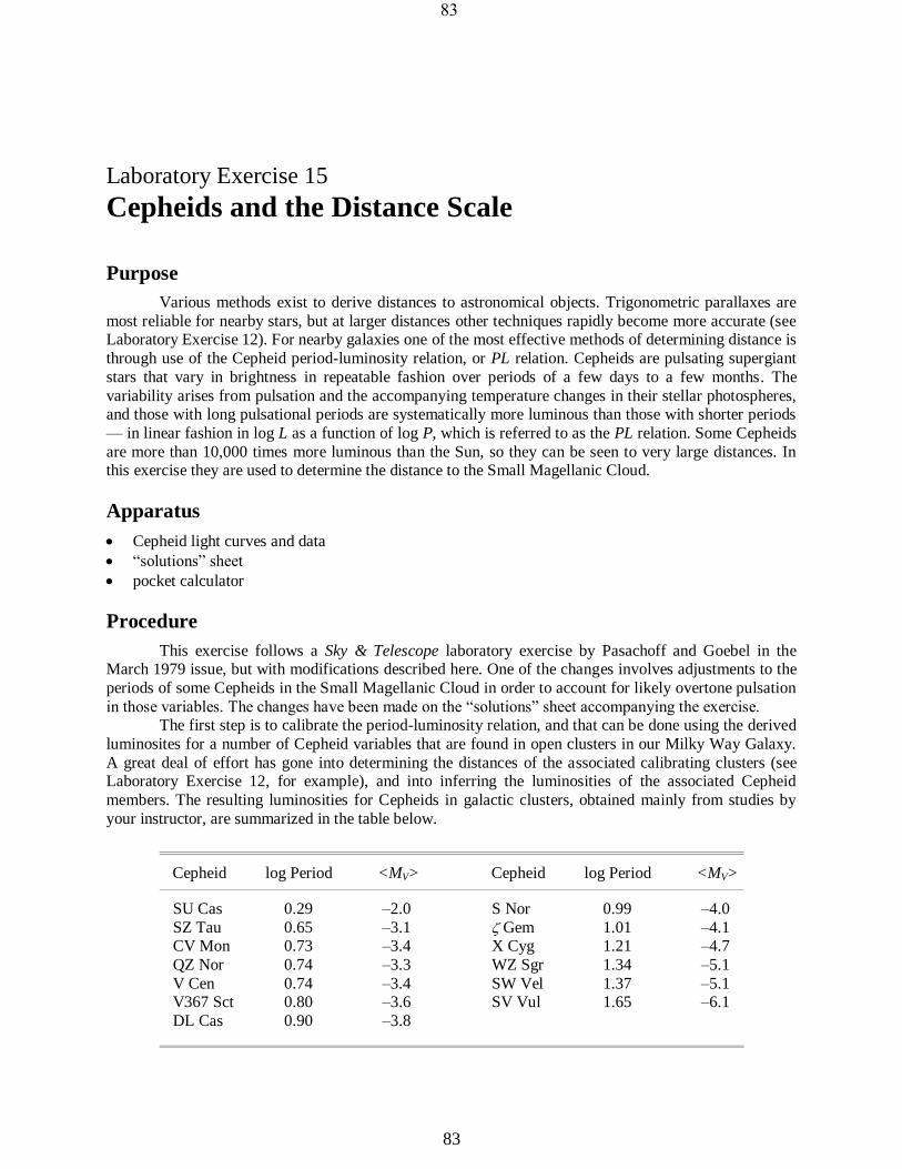
Observing Exercise 1

The Stonehenge Experiment

Purpose

This is a homework exercise intended to introduce you to some observable consequences of the

Sun’s daily (diurnal) and yearly (annual) motion across the celestial sphere. It requires a few hours of careful observing on your part at the times of local sunset (or sunrise if you prefer). During the exercise

you are duplicating a small portion of the observations made by the Bronze Age sky watchers of the

British Isles who constructed Stonehenge.

Apparatus

drawing pad (or overhead transparencies)

pen or pencil

protractor (for measuring angles)

observing site with a clear view of the western (or eastern) horizon)

Procedure

Locate a suitable site from which you have a relatively unobstructed view of the western (or, for

sunrise observers, eastern) horizon. Use the site as a fixed base for your observations, which entail carefully constructed, neatly labelled drawings to illustrate clearly the objects visible along the horizon.

Be as accurate as possible in making your observations. Best results are generally obtained by: (i) using a

ruler held at arm’s length to accurately scale the sizes and separations of objects in the field of view, (ii)

using a fixed window site with overhead transparencies and drawing pens to make accurate sketches of the visible horizon, or (iii) taking photographic exposures with a permanently mounted tripod on the

different dates.

NOTE. DIRECT SUNLIGHT IS VERY HARMFUL TO UNPROTECTED EYES. AVOID

STARING AT THE SUN FOR ANY LENGTH OF TIME DURING THE OBSERVATIONS. THE

SUN’S LOCATION IN THE SKY CAN BE DETERMINED FAIRLY ACCURATELY FROM

BRIEF INDIRECT SIGHTINGS ALONE.

Use the objects visible from your observing site as reference points, and plot the location of the

Sun in the sky as it sets, making note of the times for individual observations and the date for each

sequence. You should start about 30 to 45 minutes prior to sunset (or at sunrise and for 30 to 45 minutes thereafter) and record the Sun’s location at intervals of about 5 or 10 minutes, including the instant of

sunset (or sunrise) itself. Each drawing should include the following: date, location of your observing site,

correct times for each observation (AST or ADT) including sunset (or sunrise), the Sun’s location plotted

or shown on your drawings or photographs at those times, a dashed line to connect the individual observations for that day (i.e. the Sun’s path as it sets or rises), and the identification of specific features

on the horizon that served as reference points. All of the listed items are used to grade the exercise, so

omit them at your peril! You will need to make sunset (or sunrise) observations on at least two separate dates, preferably

separated by about a week in time, in order to detect the effects of annual motion. Observations on only

one date are not sufficient to answer all of the questions accompanying this exercise. You may also do the

10

10

experiment in small groups if you wish, although each individual in the group is required to submit a

separate account of the events as well as separate responses to the questions. You may even take along an “observing assistant.” Sunset observations for ASTR 1100 are an excellent excuse for a date!

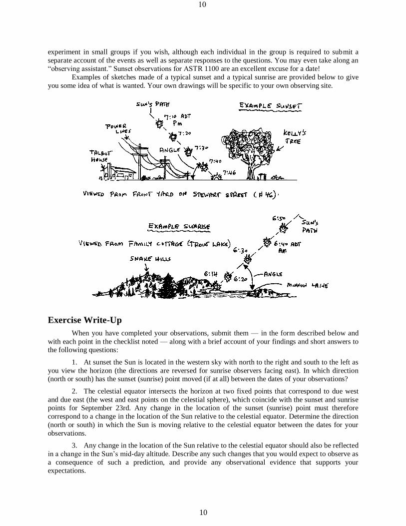
Examples of sketches made of a typical sunset and a typical sunrise are provided below to give

you some idea of what is wanted. Your own drawings will be specific to your own observing site.

Exercise Write-Up

When you have completed your observations, submit them — in the form described below and

with each point in the checklist noted — along with a brief account of your findings and short answers to the following questions:

1. At sunset the Sun is located in the western sky with north to the right and south to the left as

you view the horizon (the directions are reversed for sunrise observers facing east). In which direction (north or south) has the sunset (sunrise) point moved (if at all) between the dates of your observations?

2. The celestial equator intersects the horizon at two fixed points that correspond to due west

and due east (the west and east points on the celestial sphere), which coincide with the sunset and sunrise points for September 23rd. Any change in the location of the sunset (sunrise) point must therefore

correspond to a change in the location of the Sun relative to the celestial equator. Determine the direction

(north or south) in which the Sun is moving relative to the celestial equator between the dates for your

observations.

3. Any change in the location of the Sun relative to the celestial equator should also be reflected

in a change in the Sun’s mid-day altitude. Describe any such changes that you would expect to observe as

a consequence of such a prediction, and provide any observational evidence that supports your expectations.

11

11

4. The Sun’s path at sunset (sunrise) makes a specific angle with respect to the horizon (see

example sketches). Does the angle appear to change with time? Use a protractor to determine the approximate size of the angle in degrees.

Observing Exercise Check List

date for each set of observations

location of your observing site

correct times for individual observations including sunset (or sunrise)

the Sun’s location plotted at those times

a dashed line to connect the individual observations for each date

the identification of reference points on the horizon

12

12

13

13


Planetary Motion

Purpose

This is a homework observing exercise that is intended to introduce you to the constellations of

the Winter Sky and to the observable motions of a superior planet. Many centuries before the height of the Greek influence in astronomy, observers of the night sky knew of five celestial objects, in addition to

the Sun and the Moon, which wandered across the background of stars. Those objects are called planets,

from the Greek word for wanderers. They follow nearly the same path as the Sun and the Moon, generally

moving from west to east in the sky near the ecliptic relative to the fixed stars. Such motions of the planets is usually quite slow, and should not be confused with the daily (or diurnal) east-to-west motion

of the entire sky resulting from the Earth’s rotation on its axis.

Sometimes planets appear to move backwards in the sky, that is, in an east-to-west direction relative to the fixed stars. Such east to west motion is called retrograde motion, whereas west to east

motion is called direct or prograde motion. Planets appear to make slow loops in the sky relative to the

fixed stars during the retrograde phase. That occurs when the planet is opposite the Sun in the sky for superior planets (Mars, Jupiter, and Saturn) visible to the unaided eye. In the present exercise you are to

observe planetary motion for yourself either by making regular observations of one of the bright and easy-

to-find planets or by using The Starry Night® software that comes with the course textbook.

Apparatus

ecliptic star chart (provided)

calibrated “hand” gauge (see below) or transparent ruler to measure angular separations

sharp pencil

warm clothes

clear weather, and/or The Starry Night® software (for optional method)

14

14

Procedure

Take advantage of any clear nights available to go outside and observe either one or more of the

planets that are visible. The exact location of the planet on the star chart provided can be determined by means of triangulation with respect to stars in the same field. The major difficulties to be overcome are

the identification of the constellations and their bright stars, and the proper calibration of your measuring

device. While a properly calibrated “hand” gauge may allow you to pinpoint the separation of a planet

from surrounding identified stars on each night, you will more likely have to exercise your own creative skills in using other means to locate the planet on the star chart provided. One trick is to use a transparent

ruler to “scale” the position of the planet relative to stars you have identified, and then to transfer the

derived location to your ecliptic star chart. Another is to identify specific patterns that a planet makes with nearby stars, for example halfway between two specific stars, one-third of the way between one star and

another, etc. Whichever method you adopt, you must include a brief description of the method used on

each night. That is best accomplished by keeping a log of your observations for each night you go out. Record the dates of the observations on the ecliptic star chart provided as well as in your log.

Repeat the exercise every week or two (or even every clear night, particularly for observations of a

rapidly-moving planet) in order to obtain enough data points to answer the questions below for each

object observed.

Optional Method

Use The Starry Night® software package that comes with the course textbook to identify a bright

planet, and use the same techniques as given above (omitting the keeping of an observing log) to plot the location of the planet over a period of several months (enough to establish the entire retrograde loop).

You should plot the planet’s location on each of every other night or so, whatever seems appropriate to

avoid undue congestion on your plot. For this option you may prefer to identify only the night for specific

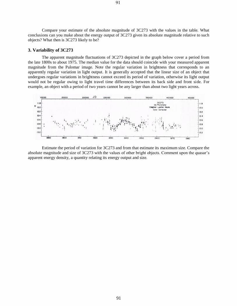
dates, e.g. October 1, 15, 31, etc. If you do select to use this option for observing planets, you should also make note of the phases

of the object on each night, i.e. record the apparent illumination of the planet’s disk. In most cases a

planet’s phases do not change significantly over a period of observation. Superior planets can only be seen in full or gibbous phases, for example. But inferior planets go through a complete cycle of phases

much like those of the Moon. That option is available with The Starry Night® software.

Questions to Answer

1. Does the orbit of the planet through the sky coincide with the ecliptic (the centre line of the ecliptic star charts)? If not, how far in degrees does it stray from the ecliptic? That value indicates the tilt

of the planet’s orbit relative to the orbit of the Earth.

2. What is the current direction of motion of the planet (as of the date you handed in the completed observing exercise)?

3. Roughly what amount of the sky (in degrees) did the planet pass through during the period of

observation?

4. Part of the exercise is to familiarize you with the bright winter constellations. How many

were you able to recognize?

15

15


The Moon’s Motion

Purpose

This is a homework observing exercise that is intended to introduce you to the constellations of

the Winter Sky and to the observable motion of the Moon from one night to the next. Observers of the night sky are familiar with seven celestial objects that wander across the background of stars. One of them

is the Moon. During the course of an evening, or even over the course of a few minutes, it is possible to

observe both the diurnal (daily) motion of the Moon, caused by the Earth’s rotation, and the orbital

motion of the Moon about the Earth. The orbital motion of the Moon is quite rapid, since it moves by more than 13º over the course of one day. In the present exercise you are to observe the Moon’s orbital

motion for yourself either by making regular observations of the Moon every clear evening or by using

The Starry Night® software that comes with the course textbook.

Apparatus

ecliptic star chart (provided)

calibrated “hand” gauge (see Observing Exercise 2)

transparent ruler to measure angular separations

sharp pencil

warm clothes

clear weather, and/or The Starry Night® software (for optional method)

Procedure

Take advantage of any clear nights available to go outside and observe the Moon. Because the

Moon’s location in the sky varies with its phase of illumination, it may be easiest to begin observations near First Quarter phase, when the Moon is located in the early evening sky. The exact location of the

Moon on the star chart provided can be determined by means of triangulation with respect to stars in the

same field. The major difficulties to be overcome are the identification of the constellations and their bright stars, and the proper calibration of your measuring device. While a properly calibrated “hand”

gauge may allow you to pinpoint the separation of the Moon from surrounding identified stars on each

night, you will more likely have to exercise your own creative skills to use other means of locating the Moon on the star chart provided. One trick is to use a transparent ruler to “scale” the position of the Moon

relative to stars you have identified, and then to transfer the derived location to your ecliptic star chart.

Another is to identify specific patterns that the Moon makes with nearby stars, for example halfway

between two specific stars, one-third of the way between one star and another, etc. Such a method can be difficult to apply near Full Moon, since the sky glow surrounding the Moon can be so bright that even

bright stars are difficult to make out. Whichever method you adopt, however, you must include a brief

description of the method used on each night. That is best accomplished by keeping a log of your observations for each night you go out.

Record the dates of the observations on the ecliptic star chart (as indicated by the initial

observations provided to you) as well as in your log. Repeat the exercise every clear night in order to obtain enough data points to answer the questions at the end of the exercise.

16

16

Optional Method

Use The Starry Night® software package that comes with the course textbook to locate the Moon,

and use the same techniques as given above to plot the location of the Moon over a period of roughly two months or so (enough to establish the entire orbit). You should plot the Moon’s location on each of every

other night or so, whatever seems appropriate to avoid undue congestion of your plot. For this option you

may prefer to use the same time for each date of observation, in which case you can turn off the Sun and

daylight to allow bright stars to be visible. If you do select to use this option for observing the Moon, you should also make note of the phase

of the Moon on each date of observation, i.e. record the apparent illumination of the Moon’s disk. That is

an option available with The Starry Night® software. Those observing either with the unaided eye or with The Starry Night® software can easily make such a record. That is, provide sketches of the Moon’s

appearance for each night that it is observed.

Questions to Answer

1. What is the inclination of the Moon’s orbit to the ecliptic according to your observations of its orbit?

2. What is the length of the synodic month according to your observations, i.e. what is the

number of days (nights) that elapsed between dates when the Moon was in the same phase, for example First Quarter phase?

3. What is the length of the sidereal month according to your observations, i.e. what is the

number of days (nights) elapsed between dates when the Moon was at the same point in the star chart?

4. Eclipses of the Sun and Moon can only occur when the Sun passes through the region near

the nodes of the Moon’s orbit. Now that you have established the Moon’s orbit from observation, you can

identify the nodes from where the orbit crosses the centre line of the ecliptic star charts. The corresponding dates specified on the ecliptic portion of the star chart indicate when the Sun will be at that

location. According to your observations, when is the next eclipse season expected?

17

17


Star Trail Photography

Purpose

The object of this exercise is to photograph star fields using a 35-mm camera, and to make use of

the resulting images to identify specific constellations and bright stars, as well as to correlate star colours with spectral types. Examples are available. The camera equipment needed is fairly standard, but you may

need to find a friend or acquaintance to borrow the necessary items. The Department of Astronomy and

Physics does not have equipment available for loan.

Apparatus

a 35-mm camera with a standard 50-mm lens

a sturdy tripod that will mate with the camera, or some other means of rigidly mounting the camera to

image the sky

a cable release to lock open the shutter of the camera for time exposures

35-mm film (for black and white shots, Kodak T–MAX 400 film or the equivalent is recommended

— for colour shots any 400 ASA film should suffice)

Procedure

Set up your camera on a tripod at your chosen observing site, and use clear nights to photograph

two or three constellations using short exposures. Good star trails can be obtained with exposures of 10–

30 minutes. Any longer and you risk building up the background sky glow, particularly if your site suffers

from light pollution. Keep an accurate record of the date and times for your exposures, as well as of your observing location. You should then be able to identify a few stars on the prints by making use of The

Starry Night® software to correlate where the camera was pointing with an image of the sky at the same

instant. You can record short star trails for just about any constellation, but you will need longer star trails when the camera is pointed towards the north celestial pole. Try to identify a range of stellar colour on

your photographs. Can you correlate the observed colours with the known spectral types of stars?

Reference to the Observer’s Handbook will help answer that question.

General Guidelines for Success

Avoid areas near the centre of cities if possible. The darker the site the better.

Avoid times when the Moon is up and relatively bright (First Quarter to Last Quarter).

Be sure you know how to use the camera properly. In particular, become familiar with the time-

exposure option that most cameras have. Also learn how to use the shutter timer if your camera has

one. That feature opens the shutter after a few seconds delay, allowing time for the vibration caused

by touching the camera to subside. If your camera does not have a timer, you can achieve the same result by holding dark cardboard just in front of the camera lens for a few seconds after opening the

shutter.

Your results will be more interesting if you know what the camera was pointing at when the image

was taken. Try using The Starry Night® software or the Department’s monthly sky charts to identify the constellations you are imaging.

18

18

Suggested Exposure Times

Be sure the lens is wide open during the exposure, which means that the f–stop should be adjusted to its lowest value. Of course, the focus should always be set for infinity. Under such conditions

exposures around 30 seconds are good for making recognizable photos of star patterns. Longer exposures

of up to 30 minutes will record the arc-like paths caused by the Earth’s rotation.

Write-Up

Submit your best prints along with information on the exposure times and other camera settings.

Indicate the dates and times of your observations and the location of the observing site. Summarize

weather information, and briefly discuss the procedure you followed. Identify the constellations and the brightest stars on your prints.

19

19


Observing the Surface of the Sun

Purpose

The object of this exercise is to observe the solar photosphere and to generate regular records of

active regions in the photosphere. From such records it is possible to learn a lot about the properties of features on the Sun, as well as about the Sun’s rotation.

Apparatus

a telescope equipped with either a solar filter or a means of solar projection (either the 0.4-m reflector

in the Burke-Gaffney Observatory or one of the Department’s portable telescopes)

recording paper pre-drawn with a circle representing the Sun’s disk

pen and pencil

Procedure

Before attempting this project you should read the section of your textbook that discusses the

Sun’s surface features. You will then be prepared to record intelligently the view through the telescope.

You should not expect to see immediately all of the features described in the textbook. Prominences and sunspots are transitory — none may be visible when you are observing. That is one reason why you are

expected to observe on several occasions. Some features, such as granulation, are not easy to observe

visually. The solar photographs in your textbook were made with large special-purpose telescopes, and

are therefore somewhat misleading as examples of what you can expect to observe. Make careful sketches of the view through the eyepiece. Standard observing sheets can be used,

or you may prefer to use your own sketchpad, pre-drawn with a circle representing the Sun’s disk. Use a

soft lead pencil and try to shade your sketch to illustrate the different brightness levels in the image. If the telescope is equipped with a Hydrogen-alpha filter (H), you will be observing in deep red light, so

everything will appear the same shade of red.

Your sketches should be accompanied by various items of supplementary information. Report the dates and times of your observations. Mention which telescope was used (there are various possibilities

for solar observing), and which filter was used. Try to identify the types of features you observed. Use the

known diameter of the Sun’s disk (32 arcminutes — 32 ,́ or 1,392,000 km) as a yardstick to estimate the

actual sizes of some of the features in kilometres. Sunspots sometimes last for a month or more, so you may observe the same ones on different dates, although in different locations since spots take only two

weeks to traverse the visible hemisphere of the Sun.

Questions to Answer

1. Did you detect the photospheric limb-darkening during your viewing sessions? What physical

process is responsible for the phenomenon?

2. How large (in kilometres) are the various features — i.e. sunspots — you observed in the solar photosphere? How do they compare in size to the dimensions of the Earth?

3. How active was the Sun during your period of observation? How will that change with time?

20

20

21

21


Observing with the 0.4-m Telescope

Purpose

The goal of evening observing sessions with the 0.4-m reflecting telescope of the Burke-Gaffney

Observatory is to obtain images of at least two different types of objects that can be viewed through the telescope, something that requires more than one observing session. You are expected to relate your

observations to the knowledge of such objects gained in class. Telescopic views and images do not

always record the same information that is provided in some textbook images, so the project is in part a

learning exercise as to what exactly can be detected with a small telescope

Apparatus

0.4-m reflecting telescope equipped with CCD camera

recording paper pre-drawn for telescope observing

pen and pencil

warm clothing

Procedure

The Telescope Operator will set the telescope on selected objects that can be imaged with the CCD camera, unless you have a good alternative object in mind (if so, you are expected to provide co-

ordinates and other information to the Telescope Operator). Images obtained with the CCD camera will

be made available to you later. For extended objects that cannot be imaged with the camera, be prepared

to sketch the field of view through the telescope eyepiece. When sketching, try to shade the sketch to indicate different brightness levels in the object. If you are looking at a star cluster, indicate brighter stars

using larger dots (the custom for astronomical sketching). Try to produce a realistic impression of what

you saw. Indicate the orientation of your sketch by locating the directions north (N) and east (E) at the appropriate points on the edge of the drawing, and note the time and date of each observation.

Write-Up

You should provide supplementary information about each object on a separate sheet along with each sketch. Describe some of the general properties of the type of object you observed, and compare

your image with any existing photographs that are available of the object, either in your textbook or in

library sources. Explain what useful scientific function could be gained from imaging the two (or more)

objects you studied. Be specific. A long, drawn-out description of the specific type of object observed, as can be found in any textbook for example, is not what is wanted. Rather, your description should address

the nature of the individual object of observation, and what purpose is served, or can be served, by

imaging that object. What can be learned about the object through imaging, and how is such information of use to astronomers?

22

22

23

23


Variable Star Observing

Purpose

The object of this exercise is to make observations of a bright variable star in order to examine its

light curve. Such observations are done by thousands of variable star enthusiasts — both professional and amateur — every clear night. The observations are also useful for tackling a variety of unanswered

questions about the nature of light variability in such stars. Although a variety of bright objects could be

chosen for such a study, the easiest to observe is Cephei, the name star for the Cepheid variables.

Cepheids are stars that are used as the standard candles for determining distances to other galaxies, as well as to establish the distance scale and expansion rate for the universe.

Apparatus

finder chart for Cephei, complete with reference star magnitudes (see below)

access to a computer running Microsoft Excel

warm clothing and clear evenings

Procedure

Locate a suitable site from which you have ready access to the night sky. It is not necessary for

the site to be completely free from light pollution, although a relatively dark site is of some advantage.

The project is also completed most easily if the observing site is adjacent to your living quarters. That

way, you can obtain the necessary observations relatively efficiently by stepping outside to your observing site for a brief period — no longer than 5–10 minutes a night.

You should observe your target variable star — in this case Cephei — as frequently as possible,

since it is possible to notice differences in brightness from one night to the next. It is even possible to observe the variable on partly clear evenings by taking advantage of breaks in the clouds. Estimate the

brightness of Cephei — its magnitude — by comparing the variable with the reference stars in its

vicinity. A reference chart for the variable is provided below, but you can also obtain a smaller hand chart from the instructor that is easier to use in the field.

The eye is capable of distinguishing brightness differences of as little as ±0.1 magnitude under

the proper circumstances. Those circumstances appear to consist of (i) an observer with some experience

in observing variable stars, and (ii) eyes that are working close to the instantaneous limit of vision for night-time viewing. Thus, your observations are best done by (i) initially gaining some experience in

viewing the field and roughly estimating magnitudes so that your eyes are more properly “calibrated”

when you begin observing in earnest, and (ii) observing the star for only as long as it takes for it and the reference stars to become visible in your gradually dark-adapting eyes. If you stay out too long your eyes

will become thoroughly dark-adapted. By that time the variable will likely be several magnitudes brighter

than the limit of your vision, and you will then have great difficulty in estimating its brightness accurately. Although that seems contradictory, it is borne out by practical experience.

The simplest way to estimate the brightness of Cephei is to watch for it to appear in the field

along with the comparison stars. You should note the instants at which each of the reference stars

becomes visible in the field, from brightest to faintest. At the same time you can note where in that sequence Cephei becomes visible. Direct comparison of Cephei with its reference stars is only

24

24

possible by placing both stars symmetrically in the line of sight about the centre of your retina — the

fovea. In other words, both stars should be placed symmetrically about the direct line of sight to your eyes. That assures that the images of both stars lie on the most sensitive part of the retina, in which case

any slight differences in apparent brightness will be easy to detect. You should be able to make a

magnitude estimate for Cephei by using the known magnitudes of the stars that compare most

favourably in brightness with it (in which case you assign a magnitude to the variable equal to that for the comparison star — rounded to one decimal accuracy), or which straddle it in brightness (in which case

you assign a magnitude to the variable using linear interpolation between the magnitudes of the two

reference stars). See your instructor if you uncertain of how to proceed.

Data Compilation

You should enter each night’s observation of Cephei into an Excel spreadsheet. For that you

need to record the date and time of your observation (to the nearest minute). That information can be converted to a Julian date (a sequential running number beginning on January 1, 4713 BC) by a standard

procedure (see instructor), or through an Internet site at http://www.phy.vill.edu/astro/links/jd.htm. The

phase of Cephei can be determined from its ephemeris, which is:

JDmax = 2442756.490 + 5

d.366270 E,

where 5.366270 days is the period of variability for Cephei and E is the number of elapsed cycles from the reference time of maximum light that occurred on Julian Date 2442756.490 (= Tuesday, December 9,

1975 at 23:45:36 Universal Time). There is nothing special about that date. It is simply a convenient point

of reference.

Keep track of your observations in a format that consists of: date and time of observation, estimated magnitude (brightness), calculated Julian Date (see above), calculated number of elapsed cycles

(E), and phase of variability (from above equation). Once you have a fairly complete data set, you can

make use of the features of Excel to graph the Cepheid’s light curve.

Reference Chart

25

25

Questions to Answer

1. Examine your resulting light curve for Cephei, the plot of magnitude as a function of

pulsational phase. How would you describe the shape of the light curve, i.e. sinusoidal, asymmetric, etc.?

2. Determine as best you can where during its cycle the Cepheid went through light maximum.

Although you might expect that to occur at phase “0.00” or phase “1.00,” many Cepheids undergo slow

period changes that result in the times of light maximum drifting further and further away from the times

predicted by a linear ephemeris (the equation for JDmax given previously). Does the phase of light maximum for Cephei occur at the expected time, or slightly earlier or later? If the latter, by how much

earlier or later does light maximum occur (i.e. as a phase shift, , or in absolute terms in units of days)?

3. Were you able to observe the Cepheid on any nights when it went through light maximum or light minimum? Did you experience any problems in estimating Cephei’s brightness on those nights?

4. Given what you have learned from the course textbook about the linear relationship that

exists between the period of pulsation of a Cepheid variable and its luminosity, what would you predict for the absolute magnitude MV of Cephei according to its observed period of variability?

5. From your observations you should be able to estimate the mean brightness of Cephei

during its light cycle, i.e. a rough estimate for <V>. Based on your resulting value for <V> and the estimate for MV obtained in the previous question, you should be able to establish the distance modulus

for the Cepheid, i.e. <V> – MV (the same as m – M). How distant is Cephei in parsecs?

26

26

27

27


Independent Study

Purpose

The goal of this exercise is to give individual students the freedom to create their own observing

projects, within the constraints of rigour associated with a standard scientific exercise. Although some potential projects are identified below, the intent is for individual students to fashion their own projects

based upon some field of astronomy or astrophysics that captures their interest. Projects can be done

individually or in small groups, but it is expected that completed projects will be written up by individual

students rather than as group reports.

Potential Projects

Binocular Observations of the Moon (with an aim to making sketches of the Moon’s disk, at different

times and at different phases, and comparing the sketches with published lunar charts — in such

fashion searching for evidence of the Moon’s libration in longitude and latitude)

Binocular or Telescope Observations of Jupiter’s Galilean Satellites (with the aim of identifying the

individual moons of Jupiter and verifying that they obey Kepler’s Third Law for orbital motion)

Globular Cluster Survey (with the goal of using a telescope to make images or sketches of all globular

clusters visible from the latitude of Halifax, and then comparing the images to detect differences in

general appearance, richness, size, and resolvability)

Aurora Search (with the aim of searching for displays of the aurora borealis on clear nights, and tying

the frequency and appearance of such displays to solar activity)

Double Star Observing (with the aim of observing a variety of different double stars having different

angular separations for their components, and using the systems to infer the angular resolution of

different observing instruments on different nights)

Procedure

Create your own observing project in consultation with the course instructor. Do your own

background research on the project using available library resources, and then carry out the project with

available facilities. Your project should have specific scientific goals that will enable you to learn something from the study. Those goals must be indicated to the course instructor beforehand.

Write-Up

Write up the results of your observing exercise much as you would any other observing exercise.

Be certain to include the educational and observational goals of the exercise, a description of how it was carried out, and the results you obtained. Tie the results to the specific educational goals originally

envisaged.

Questions to Answer

1. Were you successful or not?

2. How would you redesign the exercise to make it more successful?

28

28

29

29

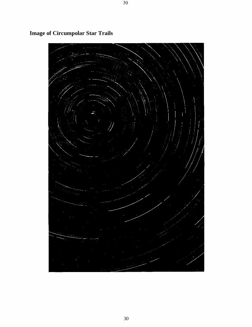
Laboratory Exercise 1

The Length of a Sidereal Day

Purpose

This exercise is aimed at determining the length of the sidereal day (the “star” day) from an

image of the circumpolar region of the sky. The length of the sidereal day is defined as the time interval between two successive transits of the vernal equinox across the meridian. It is time based upon the

Earth’s rotation on its axis with respect to the celestial sphere, or stars, rather than with respect to the Sun,

as is the case for solar time. In order to measure the length of the sidereal day, it is necessary to measure

the apparent motion of the stars around the sky. Since that is difficult to do for a full day, it is convenient to image the motion of the stars for a shorter, but well-established, time duration.

Apparatus

image of circumpolar star trails (next page)

protractor for measuring angles

“solutions” sheet

Procedure

The image depicted on the next page is a photograph of the circumpolar region obtained by Dean

Ketelsen using Tri-X film. The shutter was opened initially for 15 minutes, the lens cap was replaced for

5 minutes, and then the lens cap was removed again for a second exposure of 90 minutes duration. The

resulting star trails on the image therefore correspond to a time duration of 110 minutes from beginning to end, 95 minutes from the end of the first exposure to the end of the second exposure, and 90 minutes from

the beginning to the end of the second part of the exposure.

Measure the lengths of a variety of star trail images using a protractor, and devise a method to determine the length of the sidereal day as accurately as possible. The use of several different measures is

recommended, since that way you can obtain a mean value from several independent estimates, can

identify any obvious “outliers” in your data, and can obtain a reasonable estimate of your measuring uncertainty using the “half-the-range rule” used in PHY 205. In order to assist you, a “solutions” sheet is

provided to guide you. A sheet of polar co-ordinate tracing paper might make measurements easier, but is

not essential.

Questions to Answer

1. Does your measured value for the length of the sidereal day agree with the accepted value of

1436 minutes to within experimental uncertainty?

2. Compare your value for the length of the sidereal day with the length of the solar day, 1440 minutes. Would you expect the two values to be equal? Why or why not?

3. What is the rotational velocity of the Earth at the equator? The Earth’s equatorial radius is

6378 km.

30

30

Image of Circumpolar Star Trails

31

31


Using the Celestial Globe

Purpose

This exercise is intended to familiarize students with some of the aspects of the celestial sphere

that are represented on a celestial globe. Celestial globes are like miniature planetariums and are used to demonstrate features of the sky that are not apparent to the casual observer. Several are demonstrated in

the present laboratory exercise.

Apparatus

celestial globe (available for use only in MM 310)


Before you begin, carefully examine a celestial globe. The Department of Astronomy and Physics has a variety in the astronomy lab room, but the ones recommended for the exercise are those with shaded

plastic globes mounted on wooden bases. Each globe is free to rotate about two pivot points that represent

the celestial poles. The north celestial pole is located in the constellation of Ursa Minor at the end of the handle of the Little Dipper. The south celestial pole is located in the constellation of Octans. The

celestial equator is the great circle that runs midway between the poles, and is represented by a seam in

the plastic where the two hemispheres of the globe have been cemented together. The globe has reference lines similar to those on world globes. The lines running north-south

from one celestial pole to the other are analogous to lines of constant longitude on the Earth. They are

hour circles, all of which are great circles on the sphere. The lines that run in an east-west direction

parallel to the celestial equator are analogous to lines of constant latitude on the Earth. They are declination circles, and, except for the celestial equator itself, represent small circles on the sphere.

The globe is rectified for an observer’s location on the Earth by setting the altitude (horizon

system “up-down” co-ordinate) of the north celestial pole to the observer’s latitude. That is readily accomplished for the latitude of Halifax (45ºN) by finding the north point on the wooden base of the

globe located at azimuth 0º (horizon system directional co-ordinate), placing the north celestial pole of

the globe at that point, and adjusting the metallic band holding the globe until the 45º indicator is flush

with the wooden base (representing the horizon). The metallic band represents the observer’s meridian, which is the north-south line running through the zenith (the point directly overhead). Once the globe is

oriented, you should note the angle at which the celestial equator intercepts the east point (azimuth 90º)

and the west point (azimuth 270º). The angle relative to the horizon is 45º, which in this case represents 90º – observer’s latitude.

Procedure

1. The Sun’s annual path among the stars is represented by a series of blue dots on the globe marked 5, 10, 15, 20, 25, 30 for the corresponding calendar date of each month of the year. The line of

dots is also a great circle that intersects the celestial equator at an angle of 23º.5, an angle referred to as

the obliquity of the ecliptic. The ecliptic is the name given to the Sun’s annual path among the stars,

which does not change perceptibly from one year to another. Notice that the path is inclined to the celestial equator so that one half lies in the northern half of the sky while the other half lies in the

southern half of the sky. During the course of the year the Sun moves among the stars from a point on the

32

32

celestial equator (declination 0º) at the vernal equinox (March 21), 23º.5 north of the celestial equator

(declination +23º.5) at the summer solstice (June 22), back to the celestial equator (declination 0º) at the autumnal equinox (September 23), 23º.5 south of the celestial equator (declination –23º.5) at the winter

solstice (December 22), and back to the celestial equator at the following vernal equinox. The Sun is in

the northern half of the sky from March 21 through June 22 to September 23, and is in the southern half

of the sky from September 23 through December 22 to March 21. Find each of the equinox and solstice points on the celestial globe and record on the associated “solutions” page the designation (number) for

the hour circle passing through them. Each designation represents the right ascension of the

corresponding hour circle.

2. Take a fingertip and place it at the Sun’s location on the celestial globe corresponding to the

time of the summer solstice. Move that point so that it coincides with the eastern horizon (wooden base

for azimuth between 0º and 180º). Note on the “solutions” page the azimuth of the Sun at that instant (the

sunrise point) and the designation for the hour circle that is coincident with the meridian. You will

probably have to estimate the last value — which is the local sidereal time at the instant — by

interpolating between the two hour circles nearest to meridian. You should be able to determine the value

to within about 5 minutes of right ascension. Now move the same point (i.e. your finger on the Sun’s location) so that it coincides with the western horizon (wooden base for azimuth between 180º and 360º).

Note on the “solutions” page the azimuth of the Sun at that instant (the sunset point) and the designation

for the hour circle (local sidereal time) that is now coincident with the meridian. The difference between the local sidereal time at the instant of sunset and the local sidereal time

at the instant of sunrise is the duration of daylight for an observer in Halifax on the date of the summer

solstice. Calculate the value using the relationship given on the “solutions” page. You should also be able to estimate on the “solutions” page the compass points corresponding to the sunrise and sunset points on

that date (see attached diagram for the compass rose). Note that the points do not correspond to the east

and west points!

Now move the position corresponding to the Sun’s location (i.e. your finger on the Sun’s

location) so that it is on the meridian. Use the angular grid pattern on the metal frame to estimate the

33

33

altitude of the Sun above the southern horizon at that time. Enter the value on the “solutions” page. The

resulting value represents the Sun’s mid-day altitude.

3. Repeat the exercise from part 2 for the Sun’s location on the celestial globe corresponding to

the time of the winter solstice. Enter all values on the “solutions” page, making note of the difference in

the calculation for the duration of daylight. Sidereal time is not the same as solar time — sidereal time tracks the rate at which the stars cross the sky, whereas solar time tracks the rate at which the Sun crosses

the sky (the latter rate is slightly slower than the former) — since the Sun is moving slowly eastward

relative to the stars. But the two are close enough that your calculations for the duration of daylight are

effectively in units of solar time. Based upon the results of the exercise you should be able to describe in your own words on the “solutions” page the major differences in the Sun’s diurnal (daily) path and hours

of daylight for an observer in Halifax between the dates of the summer and winter solstices. Pay particular

attention to such details as the location of the sunrise and sunset points, the Sun’s mid-day altitude, and the duration of daylight hours on each of the two dates.

4. The celestial globe is a good tool for estimating what time of year is best for viewing various

objects of interest. Locate on the globe the three stars Deneb, Vega, and Altair, belonging to the group known as the summer triangle. The stars lie in the constellations of Cygnus, Lyra, and Aquila,

respectively. Place the group so that it is reasonably coincident with the meridian, and then note on the

“solutions” page the point on the ecliptic that coincides with the portion of the meridian (metal frame)

that lies below the horizon (under the wooden frame). That corresponds to the location of the Sun at local midnight. The corresponding calendar date (determined from the blue dots) is the date on which the

stars of the summer triangle would transit (cross the meridian) at midnight. Do you understand now why

the group is referred to as the summer triangle? Do the same exercise for the stars in the constellation of Orion. Orion is a winter constellation for

northern hemisphere observers, so it should be well placed for evening observing during the cold winter

months. Check that that is the case.

5. As a final exercise, find the constellation of Crux, the southern cross, on the celestial globe.

Now alter the setting for the altitude of the north celestial pole until all of the stars in the constellation sit

above the horizon at upper culmination (meridian crossing above the horizon). We cannot see any of the

stars in Crux at any time during the year from our location in Halifax. However, there are a few places in North America where they can be seen. Calculate the latitude for the northernmost point on the Earth’s

surface where one can see all of the bright stars of Crux, find a city in North America that lies close to

that latitude (please consult an atlas map of North America), sketch the appearance of the constellation as it would appear at upper culmination for an observer in that city (you can do that by looking through the

globe from the north side), and determine on which date the stars would be on the meridian at midnight

(i.e. what blue dot falls on the lower section of the meridian).

6. If you have time, you will find it instructive to vary the location of the north celestial pole on

the globe so that it is rectified for imaginary observers located at: (i) the North Pole (latitude 90ºN), (ii)

the South Pole (latitude 90ºS), and (iii) the Equator (latitude 0º) of the Earth. The direction in which the

stars move in their diurnal paths can be established by spinning the globe in a clockwise sense as viewed from the north celestial pole. Note how observers at the North and South Poles of the Earth are restricted

to seeing only half of the stars in the sky (a different half for each), whereas observers at the Equator get

to see all of the stars in the sky passing overhead. This is a common demonstration used in planetariums as well, except that the view of the sky is from the inside rather than the outside!

34

34

35

35


The Sidereal Period of Revolution for the Moon

Purpose

The purpose of this exercise is to determine the sidereal (orbital) period of the Moon from a series

of images showing its motion with respect to the planet Venus on April 16, 1972. The Moon undergoes two fundamental cycles: its cycle of phases (its synodic period), and its cycle of passage relative to the

stars (its sidereal period). The latter represents its true orbital period of revolution about the Earth.

Occasionally the Moon passes near a bright planet or star, which provides a good opportunity to

observe and image its angular motion in the sky. It is easy even for beginners to photograph such an event, from which direct measurements can be made to calculate the Moon’s sidereal period. In this

exercise, images of the crescent Moon passing the planet Venus obtained by Darrell Hoff from Iowa on

the evening of April 16, 1972, are used for the intended purpose. You could obtain similar images yourself, but Darrell Hoff’s images are more than adequate for the intended purpose.

Apparatus

images of the Moon taken at 7:30, 8:00, 9:00, and 10:00 p.m. (local time) on the evening of April 16,

1972 using a single lens reflex camera and a 135-mm lens with Tri-X film at f/3.5 with exposure

times of 1/30th of a second


Procedure

A visual examination of the images (following pages) reveals the rapid angular motion of the

Moon relative to the planet Venus, which is the bright spot on the right side of the images. The images were obtained with the camera facing west, and the motion of the Moon relative to Venus is eastwardly

— to the upper left in the images. Since Venus was nearly at greatest elongation east at the time the

images were obtained, it had little tangential or crosswise motion relative to Earth, and most of its motion was radial (directed along the line of sight) — see figure below. Most of the observed motion of the Moon

relative to Venus was therefore produced by the actual motion of the Moon in its orbit about Earth.

Despite that, it is still necessary to make a small correction for the motion of the Earth about the Sun

during the two and a half hours over which the images were obtained.

36

36

1. Use of sheet of tracing paper to trace the outline of the Moon from the first image at 7:30

p.m., and mark the position of the planet Venus with a plus sign (“+”) centred on the image. Move the tracing paper to each successive image, readjust the orientation so that the crescent shape of the Moon has

the same orientation as in the first tracing (there were small changes in the orientation of the camera

between exposures), and mark the position for Venus in each in the same manner as for the first image.

Your data should produce a sketch similar to that below.

Even though it is the Moon that is moving, the measurements are interpreted more easily when that motion is transferred to Venus. The image of the Moon is larger, and, and provides a more direct way

of orienting the sketch. The image of Venus is nearly a point, so it is easier to use it to trace out the

straight-line path of its relative motion.

2. Determine the scale of the images in order to translate linear measurement from the tracing

paper into angular measurements in the sky. Using a compass, trace out a full circle that best fits the

circumference of the Moon. That may involve some trial and error, but a good start can be made by

choosing a radius that is at least one half the distance between the two ends of the crescent Moon. The angular diameter of the Moon for the date of observation was 31 arcminutes (31´). Measure the diameter

(in millimetres) of the circle that best matches the size of the Moon’s disk, and calculate an image scale in

units of arcminutes per millimetre ( ́mm–1

).

3. Measure the distance (in millimetres) between each of the points representing the location of

the planet Venus at 7:30 (A), 8:00 (B), 9:00 (C), and 10:00 p.m. (D). Convert the values to arcminutes

using the image scale determined above, and obtain estimates for the angular velocity of the Moon corresponding to each of the six possible estimators: A–B, A–C, A–D, B–C, B–D, and C–D. Find the

average of the six values (the mean), and calculate the uncertainty in the result using the “half-the-range

rule” used in PHY 205. The resulting values represent your best estimate for the angular velocity of the

Moon, along with its measuring uncertainty.

4. With respect to the original drawing indicating the motions of Earth, Venus, and the Moon at

the time the images were obtained, one can see that a portion of the motion of the Moon arises can be

attributed to the orbital motion of the Earth about the Sun. The angular velocity of the Earth relative to Venus, E, is roughly that of the Earth with respect to the Sun, which equals 360° year

–1, or about 0°.985

day–1

. The value can also be expressed as E = 2 .́46 hour–1

. Add the angular velocity of the Earth to the

measured angular velocity of the Moon, , to obtain the angular velocity of the Moon relative to a non-moving Earth, 0:

0 = + E ,

where 0 = angular velocity of the Moon with respect to Earth, = measured angular velocity of the

Moon with respect to Venus, and E = angular velocity of Venus with respect to the Earth = 2 .́46 hour–1

.

5. An entire orbit for the Moon comprises 360° or 21,600 ,́ so the orbital period (sidereal

period) for the Moon is obtained by dividing 21,600´ by the value of 0 calculated above. Since the

37

37

resulting value results from a division, the uncertainty can be propagated through the calculations by

simply equating the relative uncertainty in the measured angular velocity to the relative uncertainty in the period.

Moon Images

7:30 p.m. 8:00 p.m.

9:00 p.m. 10:00 p.m.

38

38

Questions to Answer

1. Compare your resulting value for the sidereal period of the Moon with the accepted value of

27.32 days. Do the results agree, to within experimental uncertainty?

2. What are some possible sources of error in your work? Estimate the magnitudes of such errors,

and determine how they will affect your value for the Moon’s sidereal period.

3. How would your result be affected by not correcting for the Earth’s orbital velocity about the Sun? Calculate the Moon’s period without the correction, and compare your result with the known value

of 29.53 days for the synodic period of the Moon. Discuss your results.

39

39


The Orbit of the Planet Mercury

Purpose

This exercise makes use of observations for the planet Mercury to determine the size and shape of

the planet’s orbit, as well as the temporal properties of the planet as it describes its orbit. The exercise repeats some of the calculations performed by Johannes Kepler when he formulated his laws of planetary

motion. Kepler made his discoveries about planetary orbits while determining the orbit of the planet

Mars, and later extended his analysis to the other known planets. The present exercise demonstrates the

same principles applied to the planet Mercury.

Apparatus

protractor for measuring angles

millimetre ruler (a transparent ruler works best)

sharp (!) pencil


Procedure

1. Observational Material

Using the records of Tycho Brahe (the astronomer with the metal nose and aggressive drinking

habits), Kepler was able to calculate the maximum angular distance from the Sun reached by Mercury

during its orbit about the Sun. You could make similar observations yourself, but to save time a list of such angles, called maximum elongations, is given in the table below. The data were taken from the

Observer’s Handbook for the years 1967 to 1969. Similar data could be obtained from more recent

editions of the Handbook. The data tabulated give the date on which Mercury was at its maximum elongation from the Sun, its angular distance from the Sun (in degrees), and the direction of the planet

relative to the Sun.

Maximum Elongations of Mercury

Date Elongation Date Elongation

February 16 1967 18º east September 20 26º east March 31 28º west October 31 18º west

June 12 25º east January 13 1969 18º east

July 30 20º west February 23 26º west

October 9 25º east May 6 21º east November 18 19º west June 23 23º west

January 31 1968 18º east September 3 27º east

March 13 27º west October 15 18º west May 24 23º east December 28 19º east

July 11 21º west

40

40

2. The Orbit

The diagram below illustrates the orbit of the Earth as drawn on a flat surface, with dates marked

to represent the Earth’s position in its orbit throughout the year. The scale below the orbit is in

astronomical units, A.U. The Sun is considered to be located at the centre of the Earth’s orbit for this

exercise.

Astronomical Units (A.U.)

A critical feature of this exercise is that, when you draw on the diagram, you should be sure to

use a very sharp pencil so that you obtain the most precise results possible. Carelessness in this aspect of

41

41

the exercise results in poor results later, since the width of a sharp pencil line at this scale is about

150,000 km! Plot each of the elongations on the diagram as follows:

i. Locate the date for the maximum elongation on the orbit of the Earth, and draw a light

pencil line connecting that point to the Sun (the centre of the circle), as illustrated below.

ii. Centre a protractor at that point in the Earth’s orbit (the point where the light pencil line intersects the circle representing Earth’s orbit) and draw a straight line that deviates from the Earth-Sun

line by an angle exactly equal to the maximum elongation of Mercury on that date (see below). Note:

Eastern elongations occur to the left of the Earth–Sun line that you have drawn and western elongations occur to the right of the Earth–Sun line.

iii. Extend the line well across the diagram, but not so far that it intercepts the Earth’s orbit

again (see below). The line you have drawn represents the direction to Mercury on that date. As you draw more and more lines you will see the orbit taking form. When you have used all of

the data, lightly sketch the complete orbit of Mercury about the Sun (again using a sharp pencil). The

orbit must be a smooth ellipse that just touches each of the elongation lines you have drawn. The orbit

does not cross any of those lines.

An example of how to draw the line for greatest

elongation east on February 16, 1967.

An example of how to draw the line for greatest

elongation west on March 13, 1968.

Questions to Answer

1. Measure the semi-major axis, a, of Mercury’s orbit from your graph, i.e. one-half of the

maximum diameter of its orbit. Express the value as a fraction of an astronomical unit using the scale of the orbit along the bottom of the page. Compare your value with the expected value of 0.387 A.U. Do the

results agree, or do they differ significantly?

2. Calculate the expected value for the orbital period of Mercury using Kepler’s Third Law and

your observed value for the semi-major axis of the orbit, a:

i.e. P2 (years

2) = a

3 (A.U.

3) .

Compare your result with the accepted value of 0.2408 year. Do the results agree, or do they differ significantly?

42

42

3. Use the data given in the Table on the first page to calculate the synodic period of Mercury in

days. The synodic period refers to intervals between identical phases of the planet, such as greatest elongation east to greatest elongation east, or greatest elongation west to greatest elongation west. You

will need to use as many estimates of the parameter as there are estimating pairs available in the Table

(exactly 17 pairs!). Be very careful about calculating elapsed days between like phases. The year 1968

was a leap year in which there were 29 days in February. Find the average of the 17 possible values in order to get the best estimate of the synodic period. Compare your value with the textbook value of

115.85 days. Do the results agree, or do they differ significantly?

4. Measure the eccentricity, e, of Mercury’s orbit as follows:

a. Find the centre of the ellipse representing Mercury’s orbit by bisecting the major axis.

The distance from that point to the Sun’s position is the centre distance of the ellipse, c. Be sure to express the value as a fraction of an astronomical unit. Calculate the ratio:

a

ce 1 .

b. Plot the minor axis of the ellipse for Mercury’s orbit by drawing a line perpendicular to

the major axis (at an angle of 90º to it) from the centre of the ellipse. Measure the semi-minor axis, b, of

Mercury’s orbit from your graph, i.e. one-half of the minor diameter. Once again, the value should be expressed as a fraction of an astronomical unit. Calculate the parameter:

2

2

2 1a

be .

Compare e1 with e2. If the orbit is truly an ellipse, the two values should be identical and

also equal to the known value of e = 0.206 for Mercury’s orbit. Do the results agree within reasonable uncertainty limits, or do they differ significantly?

5. From what you have accomplished in the exercise, you should have a better appreciation for

Kepler’s work centuries ago. Are your values close to the textbook values, or are there differences that would make it difficult for you to confirm Kepler’s laws from the observations? What would you do to

improve upon the results you obtained in this exercise?

43

43


Black Body Radiation

Purpose

The present exercise deals with the concept of black body radiation. Black body radiation is

important in astronomy because nearly all stars radiate energy in a fair approximation to that of black bodies. As demonstrated in the exercise, hot stars radiate more of their energy at shorter wavelengths than

cool stars. The total energy radiated by black bodies of different temperatures can also be compared using

black body curves.

Apparatus

millimetre ruler (a transparent ruler works best)

sharp (!) pencil


Procedure

1. Black Body Radiation

One may think of a black body as a hypothetical object that absorbs all radiant energy incident

upon it and re-radiates such energy in accordance with its temperature. The scientist Max Planck, about

the year 1900, determined how the radiated energy of a black body is related to its temperature and to the

wavelength of the radiation. The Planck equation specifies the amount of energy E radiated at a

wavelength by a black body of temperature T (in degrees Kelvin) as:

scm

ergs

1e

12),(

35

2

kThc

hcTE

,

where h is Planck’s constant, k is the Boltzmann constant, c is the velocity of light, and e (= 2 .71828…)

is the base for natural logarithms. Although the equation above is not used for any calculations in the

present exercise, you should notice that it specifies that a black body with a temperature other than zero must radiate some energy at all wavelengths.

If the temperature of a black body is given, it is a simple matter to use the Planck equation to

calculate E, the amount of energy radiated at any given wavelength in each second by one square

centimetre of its surface. A plot of E as a function of wavelength results in a black body curve such as the one depicted in the graph on the next page. The continuous line is a black body curve corresponding

to a temperature of T = 5000 K. The table below contains the data used to construct the curve, as well as

data for two other black bodies with temperatures of 5500 K and 6000 K. Plot the data for the two other

black bodies on the graph on the “solutions” page, and sketch in smooth curves to connect the plotted points. The wavelengths are specified using Ångstrom units (Å), and one unit of energy E in the table and

graph represents 1013

ergs cm–2

s–1

of energy for each centimetre interval of wavelength.

Notice that, at a wavelength of 1000 Å, the amount of energy radiated by all of the objects is so small that one cannot graph it, and it is recorded as 0.00 in the table. It should be clear, however, that the

objects must radiate some energy at that wavelength. Only at the hypothetical wavelength of 0 Å do

objects radiate no energy at all.

44

44

Graph of Black Body Radiant Flux as a Function of Wavelength

Black Body Radiation, E, as a Function of Wavelength

(Å) 5000 K 5500 K 6000 K (Å) 5000 K 5500 K 6000 K (Å) 5000 K 5500 K 6000 K

0 0.00 0.00 0.00 5500 4.00 6.46 9.63 11,000 1.83 2.38 2.96

500 0.00 0.00 0.00 6000 4.01 6.24 9.02 11,500 1.66 2.13 2.64

1000 0.00 0.00 0.00 6500 3.90 5.87 8.27 12,000 1.50 1.92 2.36

1500 0.00 0.01 0.06 7000 3.71 5.44 7.49 12,500 1.36 1.73 2.11

2000 0.07 0.24 0.73 7500 3.48 4.98 6.73 13,000 1.24 1.56 1.89

2500 0.39 1.10 2.62 8000 3.22 4.52 6.00 13,500 1.12 1.40 1.70 3000 1.05 2.52 5.21 8500 2.96 4.08 5.34 14,000 1.02 1.27 1.53

3500 1.92 4.05 7.56 9000 2.70 3.67 4.75 14,500 0.93 1.15 1.38

4000 2.75 5.30 9.14 9500 2.46 3.29 4.21 15,000 0.85 1.04 1.25

4500 3.40 6.09 9.90 10,000 2.23 2.95 3.74

5000 3.81 6.44 9.99 10,500 2.02 2.65 3.33

2. Wien’s Law

Wien’s law states that the wavelength at which the maximum amount of radiant energy is emitted

by a black body varies inversely as the temperature of the black body. Wien’s law can be derived directly

from Planck’s law. If one denotes the wavelength at which the maximum amount of energy of a black

body is radiated by max

, then Wien’s law is written as:

8

max 102897.0

T

Å.

For each black body listed in the table and depicted in the graph, estimate from the continuous curve that

you have drawn for each black body the wavelength (to the nearest 100 Å) of maximum radiant energy

45

45

emission, and enter the value on the “solutions” page. Also determine using a calculator and Wien’s law

as expressed above the individual values of max

for each black body (to the nearest Å only), and enter the

values on the “solutions” page. You should find good agreement between the two sets of numbers.

3. Stefan–Boltzmann Law

The Stefan–Boltzmann law states that the total amount of energy radiated each second at all

wavelengths by one square centimetre on the surface of a black body is proportional to the fourth power of the temperature of the black body. The exact equation is:

scm

ergs)(

2

4TTE ,

where , the Stefan-Boltzmann constant, is 5.672 × 10–5

ergs cm–2

deg–4

s–1

, and T is the black body temperature in degrees Kelvin. The total amount of energy radiated at all wavelengths corresponds to the

area under the black body curve. The greater the area under the curve, the more energy the body radiates. There are several ways to compare the total amount of radiation emitted by two black bodies at

different temperatures. One approximation is obtained by counting the number of squares under each of

the two curves and then forming the ratio of the two numbers.

Interpretation of the Black Body Radiation Curves

Examination of the three curves in the graph leads directly to the following conclusions:

1. The curves do not intersect anywhere. For example, the curve for T = 5500 K lies entirely above the curve for T = 5000 K, and likewise the curve for T = 6000 K lies

entirely above the curves for both T = 5000 K and T = 5500 K.

2. For any wavelength greater than = 0 Å, E is greater than zero.

3. The value of max

for T = 6000 K is less than the value of max

for T = 5500 K, which

in turn is less than the value of max

for T = 5000 K.

Questions to Answer

1. Suppose that star A has a surface temperature of 6000 K and star B of the same size has a

surface temperature of 5000 K. Compare the total energy emitted by star A with that of star B by counting

the squares under the appropriate curves in the graph. Estimate areas to the nearest tenth of a square unit.

2. Use the Stefan Boltzmann equation to compute the ratio of the total radiation emitted by the

two stars.

3. Calculate, using the Stefan–Boltzmann equation, the factor by which the radiation increases if the temperature of a black body is increased by a factor of three.

4. It is possible to interpret each of the previous conclusions in physical terms. For example, the

first conclusion (#1) may be interpreted as “a hotter black body (or star) emits more radiation at all

wavelengths than a cooler black body (or star).” Express each of the remaining two conclusions in physical terms on the “solutions” page.

5. Complete the following sentence on the “solutions” page: “Hot stars appear blue in colour

because they emit most of their energy at short wavelengths (in the blue portion of the spectrum). Cool stars appear red in colour because…”

6. The visible spectrum lies approximately between 4000 Å and 7500 Å. For the black body

curve of T = 5000 K in the graph, lightly shade in the appropriate area representing the visible portion of the spectrum.

46

46

47

47


The Refracting Telescope

Purpose

This is a laboratory exercise that is intended to familiarize students with some of the properties of

convex lenses as they apply to the construction of a simple refracting telescope. The manner in which a telescope gathers and focuses light from celestial sources should be better understood after you have

completed the experiments described on the following pages.

Apparatus

metre stick

optical bench

two optical lenses

adjustable lens and screen holders

cardboard mask


Procedure

1. Images Formed by a Convex Lens

You will use two lenses in the experiment. The larger lens of the two is called the objective, while the smaller is called the eyepiece.

Carefully mount the objective lens on the optical bench in its holder. (Ask for help if you are

uncertain of what to do. The lab instructor may have already done it for you.) It helps for later

calculations to line up the holder with a distinct measuring mark on the bench. Place a light source about two to three metres from the end of the bench, with its front towards the objective lens. Next mount a

white screen behind the objective. Line up the bench with the source by sighting down its length towards

the source, with your eye at the position of the screen. Locate the image of the source on the white screen and carefully bring it into focus by adjusting the position of the screen on the bench. The separation of the

screen from the objective will probably be of the order of 50 to 60 cm (~2 feet). If you cannot find the

image, it is probably because the optical bench is not aligned closely enough with the light source.

a. Once you have located and focused the image of the source on the screen, follow the

procedure described below and answer the associated questions on the “solutions” page.

1. Estimate the ratio of the actual size of the source to that of its image. One way to do that is by

measuring the size of both with a ruler. 2. Describe the orientation of the image relative to the source, as viewed from behind the screen

relative to the objective. The four possibilities are: upright and in the same orientation as the source,

upright and reversed in orientation from the source, inverted (upside down) and in the same orientation as the source, and inverted and reversed in orientation from the source. Be very careful how you describe the

image according to the above possibilities. It pays to be absolutely precise in any scientific description. If

all else fails, sketch the appearance of both the source and the image.

48

48

b. You will be provided with a piece of cardboard having a hole in it. It is known as a mask.

Hold the mask next to the objective and slowly move the hole around in front of it. Be sure that no light passing through the objective gets by the edge of the mask. Meanwhile, carefully watch the image and

answer the following questions.

1. Is the image on the screen brighter, dimmer, or about the same brightness as it was before the

mask was used? (Remember to keep the hole in front of the lens.) Explain what might produce any change in image brightness.

2. When the hole is placed directly in front of (or directly behind) the objective lens, does the

image remain complete, or does part of it disappear? Move the hole around next to the lens and describe how the motion affects the completeness of the image. What can you conclude from the experiment about

how lenses form images?

3. Does moving the mask around cause the image to move appreciably — i.e. by the same amount as the size of the hole in the mask?

4. Does the presence of the hole in the mask cause the edges of the image to become noticeably

sharper or fuzzier?

2. The Focal Length of a Convex Lens

The focal length of a convex lens is the distance between the lens and its image when the source is (essentially) an infinite distance away. It is easy, therefore, to find the focal length of any lens by

viewing something very remote, like the Sun or the Moon. That is not easy to arrange for our exercise,

however, so we will use another method to estimate the focal length of the objective.

As the source is moved towards the lens from a large distance, the image formed by the lens moves progressively further from the lens, beyond its focal length. If the lens-image separation is called i

and the lens-source separation is called o, then the focal length of the lens, which we call f, is given by the

thin lens equation:

oif

111 .

You can use the equation to estimate the focal length of the objective.

a. Be sure that you see a sharply focused image on the white screen. Next measure the distance from the objective to the source using a metre stick. Estimate the distance to the nearest millimetre, and

record the value on the work sheet. The resulting quantity is the lens-source separation o.

b. Next estimate the lens-image separation i by using the scale on the optical bench. Assume that the objective and white screen are both centred in their mounts. Record the location of both sides of

each mount to the nearest half-millimetre, and find the average position of each mount. The value of i is

the difference between the average positions. Record all of the measurements, the average positions, and the final value of i on the work sheet.

c. Solve the thin lens equation to find the focal length of the objective. If you are uncertain of

how to do the calculations or need a pocket calculator, please ask the lab instructor for help. The manufacturer of the objective lens you are using states that the lens has a focal length of 500 millimetres

(although the actual value may differ depending upon what lens is used for the objective), and your

answer should be reasonably close. If you are not within 20 millimetres of the expected result, check your

measurements and calculations.

d. Find the percentage difference P between your result and the accepted value for the focal

length of the objective. The percentage difference is given by:

valueaccepted

valueacceptedvaluealexperiment%100

P .

49

49

3. A Simple Refracting Telescope

After removing the white screen and its holder, carefully mount an eyepiece lens on the optical

bench behind the objective. The focal length of the eyepiece is 150 millimetres (although the actual value

may differ depending upon what lens is used for the eyepiece). The correct location of the eyepiece is

behind (i.e. farther from the objective than) the position of the image by a distance equal to its focal length. Since you have found the image distance i, you should be able to place the eyepiece in roughly the

correct location on the optical bench.

You will not see an image unless the two lenses are aligned with the source. Sight down the bench from just behind the eyepiece and adjust the lenses in their holders until they are correctly aligned.

Ask for help if you need it.

If the optical components are correctly positioned, you should easily see a sharply focused image of the source by locating your eye 10 to 15 centimetres behind the eyepiece. Do not put your eye next to

the eyepiece, as you will then view the front of the optical bench rather than just the light from the

objective!

Because the eyepiece is rather small and the source is not very far from the objective, you may not be able to view the entire image at one time if, for example, you place your eye about 20 centimetres

from the eyepiece. The entire image is there nevertheless. Place your eye about 20 centimetres from the

eyepiece, and move the eyepiece sideways and up and down in order to verify that you can view all of the image even at that distance.

After locating the image proceed with the following exercises:

a. Describe the orientation of the image with respect to the source as in part 1(a) 2.

b. Position yourself so that you can view the source with one eye while simultaneously viewing

the image of the source with your other eye. Estimate the ratio of the apparent size of the image to the

apparent size of the source. The most effective way is to place a ruler in the common field of view of both

eyes and to measure the apparent sizes of the image and the source relative to the ruler scale. Your estimate of the magnification of the telescope m is defined as:

sourceofsizeapparent

imageofsizeapparentm .

c. Compute the magnification of the telescope using your value for the focal length of the objective and the given value for the eyepiece focal length, 150 millimetres. The recipe is:

eyepieceoflengthfocal

objectiveoflengthfocalm .

d. Compare the two estimates for the magnification of the telescope. Can you conclude that the recipe for m in part (c) gives a value that is reasonably close to the direct estimate from part (b)?

e. Quickly repeat the experiments in part 1b as follows. Have someone hold the mask next to

the objective and move it around slowly while you view the image. Alternatively, mount the mask in a spare screen holder and set it on the optical bench beside the objective so that the hole is next to the

objective. You can then move the mask by yourself. Try to keep your eye at the correct distance from the

eyepiece during the procedure. As the position of the mask is changed, you may have to move your eye slightly sideways or up and down to centre it on the image. Since you are looking at the same image now

as in part 1b, your results should be similar. The apparent movement of the image mentioned above, if

seen, arises from the fact that your eye is not located at precisely the correct distance behind the eyepiece.

(That location is known as the exit pupil.) Do not worry about it, as it is difficult to hold your eye in exactly the correct position during the experiment. Thus, the answer to part 1(b) 3 now depends to some

extent on factors difficult to control.

50

50

51

51


Lunar Topography

Purpose

This exercise illustrates how one can use images of the lunar surface to make actual

measurements — such as of diameter and height — for specific lunar features. The Moon has a great number of surface features available for observation. The large maria are visible with the unaided eye,

and craters are easily seen even through binoculars. With the greater magnification of telescopes and

satellite images, many other types of surface features can be identified. The shadows cast by mountain

peaks and crater walls are useful for mapping the three-dimensional lunar topography. The height of such features can be determined by triangulation once the shadow length and the local altitude of the Sun have

been measured.

Apparatus

image of the lunar surface

millimetre ruler

Procedure

Included below is an image of the Tycho region of the Moon taken just after First Quarter phase

by Larry Kelsey at the University of Iowa Observatory. The full-scale image has a scale of 6.12 km mm–1

,

while the image shown below has a scale of 12.24 km mm–1

. Beside the image is a finder chart that identifies the four major craters in the region: Clavius, Maginus, Tycho, and Pitatus. The uppermost part

of the image contains some of the lava plains of the Mare Nubium.

52

52

1. The Height of a Mountain or a Crater Wall

The determination of lunar feature heights is basically a two-step process. First, one determines

the height of the feature as it appears in the scale of the image (i.e. mm). That value is then converted to

the actual height of the feature on the Moon using the scale presented previously. The radius of the Moon,

for reference purposes, is 1737.9 km. In the diagram below left, let M be a surface feature whose height is to be measured. The

terminator is the sunset or sunrise line on the surface of the Moon. It is not a well-defined line, as

examination of the image on the previous page will show. It is necessary, however, to estimate its location to determine the heights of lunar features.

To understand more easily the method of measuring scale heights, visualize rotating the Moon so

that the feature M above is on the top edge of the Moon, as illustrated in the diagram above right. In the portion of the figure enlarged below, we see that triangles TOM and MAP are identical, except in scale,

since they have identical angles. The lines AP and TM are parallel, so the angle APM is equal to the

angle TMO.

The following ratios between corresponding sides of the triangles are therefore equivalent:

AP

MP

OM

TM ,

where TM represents the distance of the feature from the terminator, OM represents the radius of the

Moon, MP represents the height of the feature, and AP represents the length of the feature’s shadow. The

equation can be rearranged so that the height of the feature is on the left-hand side of the equation, namely:

OM

TMAPMP .

53

53

In order to measure the height of a feature, one must first measure the length of the feature’s

shadow, AP, in millimetres, convert that to kilometres using the scale given previously, then measure the distance of the feature from the terminator, TM, in millimetres, and convert that to kilometres using the

scale given previously. The height of the feature is then given by:

km 1737.9

(km)TM(km)AP(km)MP .

Measure heights for the following features using the above technique:

the central mountain peak of the crater Tycho

the central mountain peak of the crater Pitatus

the rightmost rim walls of the crater Tycho

the rightmost rim walls of the crater Clavius

the rightmost rim walls of the crater Pitatus

Show your calculations and enter your results on the “solutions” sheet.

2. The Diameter of a Mountain or a Crater

It is possible to measure the diameter of a lunar feature by establishing its apparent length in

millimetres in the image and then converting that to kilometres using the known scale of the image. Use

the technique to measure the diameters of the same features selected in part 1, i.e.:

the central mountain peak of the crater Tycho

the central mountain peak of the crater Pitatus

the rim of the crater Tycho

the rim of the crater Clavius

the rim of the crater Pitatus

Show your calculations and enter your results on the “solutions” sheet. Next produce properly scaled sketches of all five features as they would appear if seen in cross-

section. Compare the various features of the same type with one another, i.e. the central peak of Tycho

with the central peak of Pitatus, and the rims of the craters Tycho, Clavius, and Pitatus. Inspection of the original image of the Moon indicates that the three craters are not identical. Tycho appears to be a

relatively “young” crater because of the bright rays that originate from it on images taken at Full Moon.

Clavius, on the other hand, would appear to be fairly “old” on the basis of the numerous craters that litter its crater floor. Pitatus is somewhat more difficult to date, but must be older than the lava flows that cover

its crater floor. In terms of the central mountain peaks for Tycho and Pitatus, that of Pitatus may be

partially flooded by the lava flows that cover the interior of the crater. Is such a conclusions supported by

the sketches you have produced for the two craters?

Questions to Answer

1. This section has made a number of assumptions that may affect the result. We have, for

example, ignored the curvature of the lunar surface. Do you think that will be of any importance to the

conclusions reached here?

2. Given the results of the exercise with regard to your cross-sectional scale drawings of the features studied here, are they as rugged as they seem to appear in the image?

54

54

55

55


The Orbit of the Earth about the Sun

Purpose

This exercise introduces some of the different techniques used to infer a basic knowledge of the

Earth’s orbit about the Sun. The exercise is in three parts. Part one describes a method for determining the eccentricity of the Earth’s orbit. Part two describes a method for determining the Earth’s orbital speed.

And part three describes a method for estimating the mean distance of the Earth from the Sun, otherwise

known as the Astronomical Unit (A.U.). A variety of experiments of ever-increasing precision have

enabled us to derive a mean distance between the Earth and the Sun of 1 A.U. = 1.495978707 × 1011

metres. The value obtained in this exercise will be much less accurate.

Apparatus

images of the Sun taken near perihelion and aphelion

millimetre ruler

spectra of Arcturus taken at times of maximum and minimum approach speeds

pocket calculator

Procedure

1. Orbital Eccentricity

The orbit of the Earth about the Sun is not circular, but slightly eccentric. It means that the actual

distance of the Earth from the Sun varies according to what part of its orbit the Earth is in at the time. The semi-major axis a of an ellipse of eccentricity e, the aphelion distance of the Earth from the Sun ra, and

the perihelion distance of the Earth from the Sun rp are related through the equations:

ra = a(1 + e) and rp = a(1 – e) .

The semi-major axis for the Earth’s orbit can therefore be expressed as:

2

pa rra

, while the orbital eccentricity is given by:

pa

pa

rr

rre

.

Since the angular size of the Sun varies inversely as the distance of the Earth from the Sun, it is possible

to measure e directly from images of the Sun taken at perihelion and aphelion. The relationship using image diameter D rather than distance r is given by:

ap

ap

1

p

1

a

1

p

1

a

DD

DD

DD

DDe

. (1)

Illustrated in the middle of the next page are two images of the Sun: the left one taken on July 5th,

1994, when the Earth was at aphelion, and the right one taken on January 7th, 1995, when the Earth was

just three days past perihelion. It was not possible for the observer to obtain an image on the actual date of perihelion passage because of cloudy skies.

56

56

Measure the diameters of the two images as carefully as possible, averaging the values obtained

for a variety of different orientations of the measuring instrument (i.e. vertical diameter, horizontal diameter, diagonal diameter, etc.) in order to avoid problems arising from the stretching of the original

photographs during the printing stage. You should use a transparent ruler that is marked in millimetres,

and you should estimate the diameters to the nearest fraction (a tenth, say) of a millimetre whenever

possible. Once you have average values for Da and Dp, make use of the right part of equation (1) to obtain an estimate for e, the eccentricity of the Earth’s orbit. You should also propagate your measuring

uncertainties (i.e. how accurately you can measure the diameter) to determine the measuring uncertainty

for e. Use either the standard deviations of the mean values calculated for Da and Dp or use the “half-the-range rule” to establish Da and Dp, the measuring uncertainties in Da and Dp respectively. The final

uncertainty in e, i.e. e, is calculated using:

2ap

ap

p2DD

DDDe

.

Compare your estimate of eexp ±eexp with the published IAU value of e = 0.0167 for the eccentricity of

Earth’s orbit. Does your estimate agree with the accepted value to within experimental uncertainty?

2. Earth’s Orbital Speed

In 1842 Christian Doppler pointed out that when a wave source approaches us or recedes from us,

the apparent wavelengths of the waves change slightly. When a wave source approaches an observer, the

waves appear to be crowded more closely together, producing what appears to be a shorter wavelength for the waves. If the same source recedes from the observer, the waves appear to be more spread out,

producing what appears to be a longer wavelength for the waves. The magnitude of the effect is

proportional to the speed of the source relative to the speed of the waves. The same effect occurs for light, which can be considered as a wave phenomenon.

Doppler’s principle can also be applied to light received from stars, and can be used to determine

the relative velocity between a star and the observer. The orbital motion of Earth about the Sun produces

a changing Doppler effect on the apparent speeds of stars lying close to the plane defined by Earth’s orbit, i.e. stars lying near the ecliptic. When Earth’s orbital motion carries it toward a nearby star, the spectral

lines in the star’s spectrum are blue-shifted — they appear at wavelengths shorter than those at which

they were produced by the star. When Earth’s orbital motion carries it away from the same star, the spectral lines in the star’s spectrum are red-shifted — they appear at wavelengths longer than those at

which they were produced by the star. That allows us to determine the orbital speed of the Earth.

The effect is seen in the spectra of Arcturus reproduced on the next page. Shown here are four spectra (lower figure) and an identification grid for the comparison iron-arc lines (upper figure). The four

spectra in the lower figure consist of emission-line iron-arc spectra taken for comparison purposes (the

top and bottom spectra of the four), and two absorption-line spectra of Arcturus (the two inner spectra of

57

57

the four). The upper spectrum of Arcturus (the upper of the middle two spectral images) was taken on

July 1, 1939, when the Earth’s orbital motion carried it away from the star, and the bottom spectrum (the lower of the middle two spectral images) was taken on January 19, 1940, when the Earth’s orbital motion

carried it toward the star. The comparison iron-arc spectra were taken by briefly illuminating an iron arc

located on the telescope at the beginning and end of the stellar exposure, using a masking device to ensure

that the comparison spectrum bracketed the stellar spectrum rather than being superposed on top of it. For reference purposes, the rest wavelengths in Angstroms (Å) of the iron-arc emission lines are given in the

identification grid in the upper figure.

In dealing with line-of-sight motions, astronomers refer to speeds of approach using negative quantities, and to speeds of recession using positive quantities. The actual speed of a star obtained from

measurements of the positions of its spectral lines follows from the relation:

15

rest

restobserved skm1099792458.2 -

λv

, (2)

where v is the star’s speed, observed is the measured value for the wavelength of a spectral line in the star’s spectrum, and rest is the true wavelength of the spectral line in the absence of motion. If vE is the orbital

speed of the Earth and v* is the intrinsic space velocity of the star relative to the Sun, then the star’s

measured speed when the Earth’s motion is carrying it diametrically away from it is vA = vE + v*.

Similarly, its measured speed when the Earth’s motion is carrying it directly toward it is vB = v* – vE (see figure at top of next page), It follows that the Earth’s orbital speed and the star’s intrinsic space velocity

relative to the Sun are given by:

vE = ½(vA – vB) (3a)

and

v* = ½(vA + vB) (3b)

respectively.

58

58

Using a fine-scale ruler to measure the positions from the left edge of the diagram of each of the

iron-arc emission-line comparison lines in both the top and bottom spectra on the previous page, taking

care to measure the distance of the centroid of each line relative to the edge of the diagram. As

previously, estimate the distance to the nearest tenth of a millimetre if possible. Measure the top and bottom arc images separately, and refer measurements for the stellar lines to the top comparison lines for

the upper of the two middle spectra and to the bottom comparison lines for the lower of the two middle

spectra. Next plot the position of one set of lines as a function of their intrinsic wavelengths (given by the reference grid) using graph paper or an Excel spreadsheet, and fit the points with a straight line. [Many

pocket calculators contain statistical packages that allow you to find the slope and intercept of a straight

line that provides a “best fit” to data of this type using least squares techniques. Use of Microsoft Excel produces the same results. Your instructor will assist you if you would like to make use of such options.]

The resulting slope of the best fitting line is the scale of the spectral images in Å mm–1

(if you plot

reference wavelength in Angstroms as a function of line position in millimetres).

Make similar measurements for the two sets of absorption line spectra of Arcturus, the upper spectrum of the two corresponding to vA and the lower spectrum of the two corresponding to vB. Arcturus

is a cool star, and its spectrum contains many iron lines that have intrinsic wavelengths as indicated in the

reference grid. The lines appear slightly to the right (by slightly less than half a millimetre) of the comparison lines in the top spectrum, and slightly to the left (by slightly less than half a millimetre) of the

comparison lines in the bottom spectrum. Record your values for the positions of the sixteen iron lines

separately for the top and bottom stellar spectra. Next compute the individual positional differences for each line from the corresponding reference iron-arc emission lines (they should all be about half a

millimetre or less), and transform the values into wavelength differences using the image scale computed

above. The resulting numbers are the individual values for the parameter (observed – rest) for each line. Substitute them into equation (2) to obtain the speed corresponding to each of the sixteen spectral lines,

one set corresponding to the upper stellar spectrum, and the other set corresponding to the lower stellar spectrum. Average the results for all lines to obtain the speeds VA and VB indicated above (VA is measured

from the upper of the two middle spectra, and VB is measured from the lower of the two middle spectra),

along with their estimated uncertainties using the “half-the-range” rule.

In principle you should now be able to calculate both the Earth’s orbital speed and the radial velocity of Arcturus using equation (3). In practice the situation is complicated by the fact that Arcturus

does not lie in the plane of the ecliptic but 30°.8 away from it. Thus, both values — vE and v* — are

smaller than their true values as a consequence of foreshortening. The true values

59

59

smaller than their true values as a consequence of foreshortening. The true values are obtained by

dividing the numerical estimates above by cosine 30°.8, or 0.85896. You can now compare your estimates for vE and v*, along with their measuring uncertainties, vE

and v*, to the accepted values of 29.786 km s–1

and –5 km s–1

, respectively. Do your computed values

agree with the accepted values to within experimental uncertainty?

3. The Astronomical Unit

Once we have established the Earth’s orbital speed, since we also know its orbital period we can

find the radius of its orbit (the Astronomical Unit) from simple Newtonian mechanics. Since:

periodorbital

orbitofncecircumfere

time

distanceVelocity

for a circular orbit, it follows that:

P

Rv

2E ,

where vE is the orbital speed of the Earth, R is the radius of its orbit (= 1 A.U.), and P is the orbital period

(365.256363 days). Use the known value of P with the estimate for vE obtained in the previous section to

estimate a value for the Astronomical Unit. The appropriate rearrangement of the equation is:

PvR E2 ,

and the uncertainty in the estimate is given by:

PvR E2 .

Does your computed value for the size of the Astronomical Unit agree with the accepted value to within experimental uncertainty?

60

60

61

61


The Sun’s Rotation

Purpose

The purpose of this exercise is to examine evidence that the Sun rotates and to determine its

approximate period of rotation.

Apparatus

images of the Sun taken at the Hale Observatories during March and April 1947

tracing paper

spectrum of the Sun taken along the solar equator

Procedure

In the early 1600s Galileo first observed the Sun telescopically and discovered sunspots. His discovery was very disturbing to his contemporaries since the Sun was thought to be a perfect

“unblemished” celestial body. In his classic Letters on Sunspots, Galileo demonstrated by a very rigorous

argument that the spots were on the surface of the Sun and that their motion was evidence of solar rotation. He produced the first estimate for the period of the Sun’s rotation. In what was one of the earliest

quantitative determinations for the Sun, he found that “… they [sunspots] have in common a general

uniform motion across the face of the Sun in parallel lines. From special characteristics of that motion,

one may learn that the Sun is absolutely spherical, that it rotates from west to east around its centre, carries the spots along with it in parallel circles, and completes an entire revolution (sic) in about one

lunar month.” It was not until the late 1800s, however, that an English amateur astronomer, R. C.

Carrington, reported that sunspots at different solar latitudes require different times to complete one rotation.

We know now that sunspots are large areas of the solar photosphere that are relatively cooler, and

therefore, darker, than their surroundings. They are observed to last for a few days to several weeks, and

are often accompanied by large outbursts of optical, radio, X-ray, and charged particle radiation.

Another way to determine the rate of solar rotation is to use a spectrum taken with the

spectrograph slit aligned along the solar equator. Since one limb is approaching us, the solar spectral lines

imaged by the spectrograph at that end of the spectrogram will exhibit a Doppler shift towards more

negative wavelengths — a blue shift. Likewise, solar spectral lines from the limb that is receding from us will exhibit a Doppler shift towards more positive wavelengths — a red shift. That portion of the spectral

62

62

lines originating from the centre of the disk will not be Doppler shifted, since the rotational velocity of the

Sun at such points is directed transverse, or perpendicular, to our line of sight. The net result of the Sun’s rotation is that the spectral lines are tilted slightly with respect to lines originating in our own atmosphere

(see figure). The amount of tilt is proportional to the difference between the velocities of the two limbs,

and the period of rotation can be calculated.

The figure above shows a series of images of the Sun taken at the Hale Observatories during

March and April 1947. Cover a photograph with a sheet of tracing paper, and carefully trace the edge of the Sun’s disk. Sketch the outlines of the prominent spots, and record the date of the picture. Move the

sketch to successive images until you find one on which your spot tracing lines up with the spots visible

on the second date. Record the date for the second observation and calculate the number of elapsed days

between the images. It may be necessary to interpolate between dates, i.e. to calculate the number of elapsed days using fractions of a day. Repeat the procedure for at least two more sets of images, and

calculate the average value for the number of elapsed days.

The resulting value provides an estimate for the synodic period of rotation for the Sun, but not its actual, or sidereal, period of rotation. The two are related by:

63

63

sidsynrot

111

PPP , or

syn

syn

rot365.2564

2564.365

P

PP

,

where Psid is the orbital period of the Earth about the Sun (= 365.2564 days), and Prot and Psyn are in days.

Calculate the period of rotation for the Sun that results from inspection of sunspot images.

The two images above show a spectrum of the Sun around 6300 Å (lower image) along with a

schematic illustration (upper image) illustrating which features in the solar spectrum originate from

neutral iron atoms (Fe I) in the solar photosphere (wide black features) and which originate from molecular oxygen (O2) in the Earth’s atmosphere (narrow features). The rest wavelengths (in Å) of the

different lines are shown. Since the atmospheric oxygen lines are vertical, they provide excellent

reference features for measuring the tilt (x) of the solar iron lines. Simply measure from the top of an atmospheric oxygen line to the top of a solar iron line, and from the bottom of the same oxygen line to the

bottom of the same solar iron line. The difference is x. Measure the tilt of several solar lines — there are

about a dozen visible in the solar spectrum — being careful to follow the same procedure throughout.

Average the resulting values of x. Determine the dispersion of the spectrogram — the scale of the spectrum image in Å mm

–1 — by

measuring the positions of the various atmospheric oxygen lines from some reference feature in the

spectrum, say the left-hand edge of the spectrogram. Construct a graph that plots the wavelength of the oxygen line as a function of its measured position. The slope of the best-fitting relation is the image scale.

Use that value to convert your average value of x from millimetres to Ångstroms. Next recall the

Doppler relation from the previous exercise:

15

rest

skm1099792458.2 -

λv

,

where v is the speed of the an object, is the wavelength sift in Å just calculated, and rest is a suitably

selected rest wavelength. For the latter, choose a value appropriate for the middle of the spectrogram, or a value representative of the average for the lines studied. The resulting value for the speed, v, represents

the difference in velocity between the two limbs of the Sun along its equator — one limb of which is

64

64

receding from us and the other of which is approaching us. The rotational speed at each limb is therefore

one-half of that value. The rotational period of the Sun’s rotation at the equator can be calculated from the relationship

between the speed of rotation and the circumference of the Sun, i.e. from:

1

5

s km

km1096265.62Sun theof nceCircumfere(seconds) Period Rotational

-vv

.

Convert the resulting value for the rotational period from a value in units of seconds to a value in units of

days.

Next compare the result just obtained for Prot with the value obtained from images of sunspots. The two values may not be exactly the same because of differential rotation in the Sun. Rather than

rotating like a solid body, regions closer to the equator of the Sun rotate more rapidly than regions

towards the poles. Is there any evidence for such an effect in your calculations? Comment upon your findings.

65

65


The Hertzsprung-Russell Diagram

Purpose

The Hertzsprung-Russell (H-R) diagram is a graph that plots, for individual stars or groups of

stars, a parameter related to stellar luminosity (e.g. log L/L

, Mbol, or MV) versus a parameter related to stellar temperature (e.g. log Teff, colour index (B–V)0, or spectral type — OBAFGKM). Such a diagram is

one of the most useful graphs available to astronomers, because a star’s position in the graph provides

useful information about the star’s intrinsic brightness, temperature, distance, mass, radius, and age.

Apparatus

chart of the Hertzsprung-Russell diagram


Procedure

1. The Nearest Stars

The data available for 65 of the 72 known stars closest to the Earth are tabulated below. Plot the

data either on the graph that accompanies the exercise and that represents a typical H-R diagram, or using

your own Microsoft Excel spread sheet. Be careful to plot the individual data points as accurately as you

can. The white dwarfs are difficult to plot accurately since the corresponding temperature types in their spectral sequence are not on the same system as the others. Try to include them as best you can. Star Sp. Type MV Star Sp. Type MV Star Sp. Type MV

Sun G2 V +4.82 BD+59°1915A M3.5 V +11.18 LP731–58 M6.5 V +17.32

Proxima Centauri M5.5 Ve +15.45 BD+43°44A M2 V +10.33 CD–46°11540 M3 V +11.10

Cen A G2 V +4.34 BD+43°44B M4 V +13.34 G208–45 M6 Ve +15.70

Cen B K1 V +5.70 G51–15 M6.5 Ve +17.01 G208–44AB M6 Ve +15.12

Barnard’s Star M5 V +13.24 Ind K4 Ve +6.89 L145–141 DC: +13.18

Wolf 359 M6.5 Ve +16.57 Cet G8 V +5.68 G158–27 M5–5.5 V +15.38 BD+36°2147 M2 V +10.46 L372–58 M4.5 V +15.21 BD–15°6290 M5 V +11.80

Sirius A A1 Vm +1.45 L725–32 M5.5 Ve +14.25 BD+44°2051A M1 V +10.40 Sirius B DA2 +11.33 BD+5°1668 M4 V +11.94 BD+44°2051B M5de +15.93 L726–8A M5.5 Ve +15.42 Kapteyn’s Star M1 VIp +10.89 BD+50°1725 K7 V +8.16 L726–8B M5.5 Ve +15.82 CD–39°14192 M0 Ve +8.71 BD+20°2465 M3.5 Ve +10.99 Ross 154 M3.6 Ve +13.00 Krüger 60A M3.5 V +11.58 CD–49°13515 M2 V +10.19

Ross 248 M5.5 Ve +14.77 Krüger 60B M4 Ve +13.30 LP944–20 M9 V +17.00

Eri K2 V +6.18 Ross 614A M4 Ve +13.05 CD–44°11909 M4 V +12.43

CD–36°15693 M2 V +9.76 BD–12°4523 M4 V +11.95 2 Eri A K1 V +5.92

Ross 128 M4 V +13.50 CD–37°15492 M2 V +10.36 2 Eri B DA +11.01

L789–6ABC M5 V +14.63 Wolf 424A M5 Ve +14.89 2 Eri C M4.5 Ve +12.66

61 Cyg A K5 V +7.49 van Maanen’s Star DG +14.15 BD+43°4305A M4 Ve +11.77 Procyon A F5 IV–V +2.68 L1159–16 M4.5 Ve +14.01 70 Oph A K0 V +5.67 Procyon B DF +13.00 L143–23 M4 +15.60 70 Oph B K4 V +7.46 61 Cyg B K7 V +8.33 CD–25°10553B M1.5 +13.80 Altair A7 V +2.20 BD+59°1915B M4 V +11.97 BD+68°946 M3.5 V +10.87

66

66

As you include more and more points on the graph, you will notice that most stars fall along a

single curved band. That band is called the main sequence. The location of a star on the main sequence is specified almost entirely by its mass and its chemical composition, with differences between stars of

similar chemical composition depending almost exclusively upon differences in their masses. For

reference purposes, the masses of stars of known spectral type on the main sequence are roughly: O5 (~30

M

), B0 (14 M

), A0 (2 M

), F0 (1.5 M

), G2 (1 M

), K0 (0.8 M

), and M0 (0.5 M

). Once a star forms and begins to fuse hydrogen to helium in its core, it shines with an absolute magnitude (luminosity) and

spectral type (temperature) determined by that point on the main sequence corresponding to the amount of

matter it contains — its mass. The main sequence therefore does not represent how the parameters of stars vary as they age, which was an early idea that was discredited decades ago. Rather, as a star consumes its

core supply of hydrogen, its surface temperature drops and its luminosity increases, which moves it

upwards and to the right in the H-R diagram. That explains why some stars are found to the upper right of the main sequence.

Stars that fall above the main sequence in the H-R diagram are called giants (luminosity class III)

and supergiants (luminosity class I), which are much more luminous than main sequence stars, or dwarfs

(luminosity class V), of the same temperature. Stars that fall below the main sequence on the lower left portion are called white dwarfs, or degenerate stars, and are much smaller and less luminous than the Sun.

They are typically about the same size as the Earth. Refer to your completed H-R diagram and the

“solutions” sheet in answering the questions listed there about the nearest stars.

2. The Stars in Orion

The table below contains data for the parameters of the bright stars in the constellation of Orion. Plot the data for the stars in the graph representing the H-R diagram along with the nearest stars, but use

different symbols to denote the second group. Some stars fall above the top of the diagram, but you

should still include them using the space available above the top of the graph. The stars in Orion differ

from the group of nearest stars in that they are characterized by quite different properties — they are bright, visible to the unaided eye, and lie in one small portion of the night sky. In that sense they represent

a group of stars selected on the basis of intrinsic brightness rather than proximity to the Sun. Their

characteristics therefore differ from those of the nearest stars. Refer to your completed H-R diagram and the accompanying work sheet to answer the questions listed there about the stars in Orion. Star Sp. Type MV Star Sp. Type MV Star Sp. Type MV

Ori M2 Ib –5.14 1 Ori D B0.5 Vp –2.09 3 Ori F6 V +3.67

Ori B8 Ia –6.69 2 Ori O9.5 Vep –2.43 4 Ori B2 III –4.25

Ori B2 III –2.72 Ori O9 III –5.30 5 Ori B2 III –4.36

Ori O9.5 II –4.99 Ori B0.5 Ia –4.65 6 Ori K2 II –2.86

Ori B0 Ia –6.38 Ori O8 IIIe –4.16 Ori O9.5 V –3.96

Ori O9.5 Ib –5.26 Ori A2 Vm +0.78 Ori B5 III –2.56

Ori B1 V + B2e –3.86 Ori B3 IV –1.65 1 Ori B0 IV –3.01

1 Ori A O7 V –3.69 Ori B3 IV –2.00 2 Ori G8 III–IV +1.33

1 Ori B B1 V –1.46 1 Ori A0 V +1.53 1 Ori G0 V +4.70

1 Ori C O6 V –4.23 2 Ori A1 Vn +0.48 2 Ori B2 Ia –7.82

Questions to Answer

General

On your completed graph, sketch lightly a shaded band that represents the location of main

sequence stars (dwarfs). Since the H-R diagram in this exercise plots observational parameters (MV and

spectral type) rather than theoretical parameters (log L/L

and log Teff), the main sequence band should be

67

67

curved rather than straight. Check to see if that is the case. Next answer the following questions on the

“solutions” sheet.

1. Identify from the H-R diagram a star that is a white dwarf (degenerate star). What is the name

of the star in the tables?

2. Identify from the H-R diagram a star that is a red supergiant. What is the name of the star in the tables?

3. Identify from the H-R diagram a star that is a blue supergiant. What is the name of the star in

the tables?

4. Identify from the H-R diagram a star that is a red giant. What is the name of the star in the

tables?

5. Identify from the H-R diagram the star that is most similar to the Sun in terms of its

luminosity and spectral type (it need not be identical). What is the name of the star in the tables?

The Nearest Stars

6. Are there any giant or supergiant stars located near the Sun?

7. Identify from the H-R diagram the hottest star in the Sun’s vicinity. What is the name of the

star in the tables?

8. Identify from the H-R diagram the most luminous star in the Sun’s vicinity. What is the name

of the star in the tables?

9. Identify from the H-R diagram the coolest star in the Sun’s vicinity. What is the name of the star in the tables?

10. Roughly what proportion of stars in the Sun’s vicinity are similar to the Sun in temperature

and luminosity?

11. Are white dwarfs (degenerate stars) a common constituent of the solar neighbourhood:

a. relative to supergiant stars?

b. relative to M dwarfs?

c. relative to stars like the Sun?

12. What is the approximate mass of the most typical type of star found in the Sun’s

neighbourhood, in solar units?

The Stars in Orion

13. Identify from the H-R diagram the hottest star in Orion. What is the name of the star in the tables?

14. Identify from the H-R diagram the star in Orion that has the lowest surface temperature. What

is the name of the star in the tables?

15. For stars in Orion that fall on the main sequence, which one is the most massive? Identify it

by name.

16. Roughly what is the mass of the star identified in question 15?

17. For stars in Orion that fall on the main sequence, which one is the least massive? Identify it

by name.

18. What is the mass of the star identified in question 17?

68

68

19. What is the name and spectral type of the intrinsically least luminous star in Orion?

20. What is the name and spectral type of the intrinsically most luminous star in Orion?

21. What is the name of the largest star in Orion?

22. What proportion (percentage) of the bright stars in Orion are over 100 times (5 magnitudes)

brighter than the Sun?

23. In terms of the Sun’s radius, how large is the star in question 21? (You will have to calculate

the value using suitable values for the temperature of the Sun and the star.)

69

69


The Hyades Moving Cluster

Purpose

The purpose of this exercise is to determine the distance to the Hyades cluster independent of

trigonometric parallaxes. In the case of a moving cluster, it is possible to determine the individual distances to cluster stars using proper motion and radial velocity data, which are often established with

greater precision than trigonometric parallaxes. The technique works only if the motion of a star cluster

has a sizeable component in the line of sight. Of the various moving clusters recognized, that is the case

only for the Hyades cluster, the V-shaped group surrounding the red giant Aldeberan. This exercise demonstrates how the method is applied to Hyades stars.

Apparatus

chart of proper motion as a function of spatial location on the sky for Hyades cluster stars (provided)

pocket calculator

sharpened pencil

transparent ruler

Procedure

The Hyades cluster is of particular interest to astronomers because of its richness and close

proximity to the Sun. Cluster stars are dispersed over a fairly large area of sky, but their proper motions

and radial velocities are sufficiently well determined that they can be combined to produce a reliable

estimate for the distance to the cluster using the moving cluster method. The stars of the cluster travel through space along parallel paths, and their direction of motion is evident from their proper motions.

70

70

The graph provided plots using arrows the proper motion vectors for a large selection of Hyades

members on a rectilinear grid of cos versus , where is the right ascension (not labelled on the diagram) and is the declination (the two together are the rectilinear space co-ordinates). It would be

advantageous to have the arrows drawn to a larger scale, but that would not influence the results of the

exercise significantly since the scatter introduced by measuring uncertainties in the proper motions is

appreciable. The uncertainties can be reduced by isolating small samples of stars in different areas of the cluster and drawing proper motion vectors representative of each sample. A clear ruler produces good

results. Select stars or vectors for which the proper motions appear to represent the surrounding stellar

group, and extend the vectors towards the left side of the figure using considerable care and a well-sharpened pencil. In precise studies of the Hyades moving cluster, one must take into account that the

vectors represent portions of great circles rather than straight lines, so your results for the location of the

cluster convergent point may differ from literature findings. That need not concern you.

1. Plot as many lines (typically 20 to 30) as seem reasonable to delineate the cluster convergent

point, and tabulate the resulting values for the co-ordinates and for the location of the point that seems

closest to the true convergent point. There will be some uncertainty associated with your resulting co-ordinates because of scatter in the intersection points of the proper motion vectors. The best eyeball

estimate of the convergent point’s location should have about two-thirds of the proper motion vectors

passing within a small error circle about that point. The parameter is the angular distance of a cluster star from the convergent point. Here we also use to denote the angular distance of the cluster centre

from the convergent point. Make a reasonable estimate for the uncertainty in the location of the

convergent point using the radius of the error circle. Use the scale of the -axis to convert from millimetres (as measured with your measuring device) to angular units (degrees and decimal fractions).

2. Assume that measuring uncertainties in the stellar proper motions and radial velocities have

an insignificant effect on the uncertainty in the cluster’s distance relative to the uncertainty in specifying the location of the cluster’s convergent point. The relative uncertainty in distance d that applies under

such conditions is given by:

cossin3.57

d

d , for in degrees.

3. Estimate d/d for the Hyades cluster using the results you obtained in part 1. Adopt a value of

appropriate for the distance to the centre of the cluster by measuring the distance of the convergent point from a point located near the optical centre of the cluster (where most of the stars congregate).

Convert the value to degrees using the scale on the right axis of the graph.

4. Derive individual distances for the eight stars in the accompanying table using the given values of proper motion , distance from the convergent point , and radial velocity VR. The appropriate

formula is given in your textbook, and is:

74.4

tanRVd ,

for VR in kilometres per second, in seconds of arc per annum, and d in parsecs. Assume that the stars

have been selected at random from known cluster members (i.e. they are randomly distributed about the

cluster centre), and use them to obtain a new best estimate (including its associated uncertainty using the “half-the-range” rule) for the distance d to the Hyades cluster. Simply calculate the average value for the

individual distances, and use the “half-the-range” rule to estimate the uncertainty d.

71

71

Star VR Star VR

6 0".151 year–1

37°.5 31.6 km s–1

104 0".103 year–1

26°.0 44.4 km s–1

14 0".152 year

–1 32°.5 35.8 km s

–1 112 0".074 year

–1 24°.0 38.2 km s

–1

33 0".114 year–1

30°.5 36.1 km s–1

129 0".079 year–1

23°.5 42.5 km s–1

74 0".115 year–1

29°.0 40.5 km s–1

131 0".094 year–1

26°.5 41.3 km s–1

5. Compare the results from parts 3 and 4 in terms of both the derived distance d to the cluster

and the uncertainty d/d, noting any similarities or differences. How distant is the Hyades cluster according to your work?

72

72

73

73


Open Cluster Colour-Magnitude Diagrams

Purpose

The purpose of this exercise is to study the relative H-R diagrams (or colour-magnitude diagrams)

of three open clusters to determine their ages and distances, and to compare the method of cluster parallax with that of trigonometric parallax.

Apparatus

colour-magnitude diagrams of three open clusters (NGC 6087, NGC 6531, and Collinder 285) and a

calibrated ZAMS mounted on acetate sheets (see below)

pocket calculator

74

74

Procedure

The colour-magnitude diagram, or H-R diagram, of a star cluster allows astronomers to determine

directly some fundamental properties of open clusters, such as distance and age. The study of open clusters in general has also generated some very important results in astronomy, of which proof for the

existence of interstellar reddening and a means of calibrating the Cepheid period-luminosity relation are

but two examples.

When one compares the colour-magnitude diagrams of open clusters, an essential tool is a calibrated zero-age main sequence (ZAMS), which is the locus of points on the H-R diagram where stars

of different masses first begin to generate all of their energy through hydrogen fusion. The calibrated

ZAMS used in this exercise was generated through use of the unreddened colour-magnitude diagrams of several young open clusters, all of which have been linked to the main sequences for the Hyades and

Pleiades clusters, all corrected to a metallicity scale close to the solar value. The age calibration for the

main sequence turnoff point was tied to the results for stellar evolutionary models.

1. Distance Determination

Provided with this exercise, in addition to a ZAMS calibrated to solar metallicity and to stellar evolutionary models, are the reddening-corrected colour-magnitude diagrams for three open clusters:

NGC 6531, NGC 6086, and Collinder 285 (also known as the Ursa Major moving cluster). The method of

ZAMS fitting is to use the calibrated ZAMS to find the best-fitting match to the least-evolved main-sequence stars in a cluster. The exercise comes equipped with copies of the colour-magnitude diagrams

and the ZAMS on acetate sheets, and are all on the same scale, so it is a simple matter to match the left

and right borders of the graph for the ZAMS to the left and right borders of the graphs for each open

cluster colour-magnitude diagram, and to slide one on top of the other vertically until a good match is found for cluster main-sequence stars.

A good match is one where there is a tight fit of most of the least-luminous main-sequence stars

with the calibrated ZAMS, with all deviant points lying above the calibrated ZAMS. Do not try to match all points to the ZAMS, since that will invariably produce lots of data points lying below the ZAMS. Such

a result is nonsense for main-sequence stars, since there is no known physical mechanism for making

stars less luminous than their main-sequence luminosities. On the other hand, there are several mechanisms that can make stars appear more luminous than their main-sequence luminosities, including

unresolved binary companions, rapid rotation, and evolution away from the ZAMS. The last mechanism,

in particular, is expected to predominate for the most luminous main-sequence stars, which are closest to

the end of the hydrogen-burning stage. When a good match has been found, compare the values of V0 for cluster stars with the values of

MV for the corresponding ZAMS. Find the point on the V0-axis of the cluster colour-magnitude diagram

that corresponds to MV = 0 for the ZAMS. You should be able to identify the point to the nearest tenth of a magnitude in V0, i.e. to ±0.1 magnitude, although individual results may vary. In any case you should

record both the value of V0–MV for the cluster, i.e. the value of V0 corresponding to MV = 0, and its

uncertainty according to your ability to discern the best fit. Follow the same procedure for each cluster,

being careful with NGC 6531, since for this cluster it is the least luminous stars that deviate most from the ZAMS.

The value of V0–MV for a star cluster is equivalent to an estimate of its distance modulus, m–M.

Since the distance modulus m–M = 5 log d – 5, it follows that the distance to an open cluster in parsecs can be established from:

52.010 Mmd .

Note that the uncertainty in the distance, d, follows from the derivative of the distance modulus relation,

i.e. from:

d

d

d

d

d

deMm

1715.2

4343.05log5 10 ,

75

75

which simplifies to:

d

Mmd

1715.2

.

The value of (m–M) is just the uncertainty in the ZAMS fit that you found previously, i.e. ±0.1 or ±0.2,

or whatever, whichever value applies to you own results. Use the technique as described above to determine the distances to the three clusters, along with

their associated uncertainties. (In general, an uncertainty can only be quoted to at most two significant

figures, so your values of d ±d should be rounded appropriately at the end of your calculations. Once you have obtained distances for all three clusters, rank them in order of increasing distance. There is a

second method of determining the distance to the cluster NGC 6087, since it contains the Cepheid

variable S Normae. S Normae was observed by the Hipparcos satellite, and the star’s trigonometric

parallax was found to be 0.00119 ±0.00075 arcsecond. The distance to an object obtained from its trigonometric parallax, , is given by:

1d , with dd

.

Obtain a second estimate for the distance to the open cluster NGC 6087 using the trigonometric parallax

for its member Cepheid variable S Normae.

Questions to Answer

1. Which cluster is closest?

2. Which cluster is most distant?

3. Which estimate of distance for the cluster NGC 6087 is more precise, the method of ZAMS

fitting or the method of trigonometric parallax?

4. From the results for the previous question, what can you say about the usefulness of cluster

parallaxes?

2. Cluster Ages

In addition to a best match of the ZAMS to the main sequence for each cluster, you should also be

able to establish the cluster main-sequence turnoff point from where luminous cluster stars begin to deviate systematically away from the ZAMS. Use the age calibration with the ZAMS, which cites the

logarithm of the age in years from stellar evolutionary models for the ZAMS turnoff points, to estimate

the ages of the three clusters in this exercise. Be careful for NGC 6531. You may have to estimate where the turnoff point for the cluster lies on the basis of only one or two stars. Do not confuse its turn-on point

for a turnoff point. Once you have obtained ages for all three clusters, rank them in order of increasing

age.

Questions to Answer

5. Which cluster is youngest?

6. Which cluster is oldest?

7. Consider the Cepheid S Normae in the open cluster NGC 6087. You know the likely age of

the cluster from the cluster turnoff point. Given the location of the star in the cluster colour-magnitude diagram, however, what can you say about its stage of evolution? Comment on what is likely to be

happening in the core of the star? Is S Normae likely to be still undergoing hydrogen fusion in its core?

76

76

77

77


Spectral Classification

Purpose

Astronomers classify spectra in order to learn more about the basic characteristics of stars, such

as their temperatures, surface gravities, chemical compositions, and rates of rotation. The purpose of this exercise is to classify the spectra of five stars on the OBAFGKM system used by astronomers, thereby

establishing approximate effective temperatures for the stars. The classification is done using trailed

grating spectra of unknown stars and an atlas of representative stellar spectra.

Apparatus

stellar spectral atlases (available only in MM 310)

spectra of five unknown stars

Procedure

Presented below are grating spectra for five stars. They have all been reduced to the same scale

on the page, and have also been aligned vertically so that the Balmer lines of hydrogen are at the same locations in each spectrum. They are the sequence of spectral lines with decreasing separation to the left.

See you textbook for similar spectra. The goal of this exercise is to establish the spectral types of the stars

as accurately as possible. Once that is done, it is possible to determine the effective temperatures of the

stars using the table in the textbook.

Star 1

Star 2

Star 3

Star 4

Star 5

When you examine the spectra of stars, you notice the various vertical lines — some broad, some narrow — that are used for detailed spectral classification. They appear dark in the actual stellar spectra

since they represent a loss of light from those wavelengths, the light having been absorbed by gas atoms

to excite the atoms to higher atomic energy levels. The spectra above are reproduced from negative images of the original spectra, so they appear white against the dark gray stellar continuum. As noted

above, one particularly prominent set of lines of decreasing spacing to the left in the spectra can readily

be identified. They are the Balmer lines of hydrogen, which are visible in most spectra. In the spectra

78

78

reproduced here, the prominent lines from right to left are H, H, H, H, etc. Although the Balmer lines

are useful for spectral classification, the main criteria used for such purposes are often the strengths of weaker spectral lines of other elements, including both neutral and ionized species, seen between the

Balmer lines. The variation of their strengths with temperature is governed primarily by the Saha and

Boltzmann equations, which provide the needed physical basis for derived relationships between spectral

type and photospheric temperature. O-type stars are the hottest with photospheric temperatures of 50,000 K or more, and M-type stars are the coolest with photospheric temperatures of 3000 K or less.

The techniques of spectral classification consist primarily of tricks of visual perception that are

difficult to teach except by way of actual hands-on experience. The objective of this exercise is to introduce the field through the problem of classifying the spectra for the five stars illustrated here.

Carefully match each spectrum with one or more standards in the spectral atlas, in the process assigning a

single spectral type and subtype (e.g. A5, G8, etc.) to each star. The actual stars range over a variety of luminosity classes, from main-sequence stars of class V to supergiants of class Ib, so do not constrain

your search only to stars of one luminosity class. Although you are not expected to classify the stars in

terms of luminosity, you should be aware that such differences will effect the appearance of some spectral

lines — narrow versus broad Balmer lines in supergiants, for example — as well as their relative strengths.

You must provide a brief justification for each classification. That involves identifying prominent

lines in each spectrum and finding standard star spectra that are a good match in relative line strength to those features. Be careful however. The hydrogen Balmer lines are present in all stellar spectra, for

example, but they vary greatly in strength (width and depth) according to properties such as surface

gravity (luminosity) and rotational velocity, and not just photospheric temperature. Become experienced with the appearance of a wide variety of spectra before beginning to classify the stars in this exercise. The

resolution of the spectra is relatively low, but is sufficient to classify the associated stars visually in terms

of their different temperature classes — the O B A F G K M types — and subtypes — e.g. B2, B5, G8,

etc. Be sure to include your best estimate of the spectral subtypes for each star, and not just the main spectral class.

Your laboratory write-up should consist of a list of the stars, an assigned spectral type for each, a

detailed description for each star of why that particular spectral type and subtype was assigned, and an estimate of the star’s photospheric temperature made on the basis of its spectral type. Spectral

classification is done best by examining line ratios rather than simply the overall appearance of spectra.

Not everyone is blessed with the necessary visual acuity, so there is no reason to be concerned if your

results do not match those of your classmates. You may find, however, that discussing the spectra of specific stars with classmates or with the lab demonstrator provides insights into the proper classification

of the stars. But remember that the final classifications should be your own. Your grade will be based

upon the general accuracy of your classifications as well as your descriptions of the features pertinent to the classifications of the stars.

79

79


Investigation of a Star Field in Cygnus

Purpose

This exercise involves the exploration of a region of the Milky Way that passes through the

constellation of Cygnus. The four images used in the exercise show two adjacent areas of the sky. Each area was photographed in both red light and blue light using different combinations of film and filters.

The original photographs were made on 14 × 14-inch glass plates with the 48-inch Schmidt telescope on

Mount Palomar. A Schmidt telescope is a special type of reflecting telescope with correcting lens

designed to produce images of the highest quality showing large areas of the sky. The negative reproductions used here show stars as black images against a white background. The reproductions were

painstakingly made from the original glass negatives at the Hale Observatories, and represent a tiny part

of a larger survey of the northern sky completed by the Observatory in the 1950s using the 48-inch Schmidt telescope. The collection forms an invaluable research tool for astronomers; images such as these

are in routine use at major observatories around the world. One of their most important uses is to aid in

locating and identifying interesting stars and galaxies. There is such an overwhelming wealth of information on the images that astronomers will be discovering new and curious objects on them for years

to come. In fact, the curiosity of many astronomers often leads them to “browse” through the Sky Survey

during off-hours just to see what they will stumble across.

The prints cover a square on the sky that is six degrees (12 apparent Moon diameters) on a side, for a total of 36 square degrees per print. The scale on the prints is 67.14 seconds of arc per millimetre. At

that scale the Full Moon would appear as a circle with a diameter of 27 millimetres.

Apparatus

Palomar Observatory Sky Survey images (available only in MM 310)

grid overlays


Procedure

1. Identifying the Parameters of the Photographs

Separate the red and blue print of the two star fields. Use the fact that hot hydrogen clouds (called

H II Regions) radiate strongest at red wavelengths (the H Balmer line) to decide which print of each pair

is the one taken in red light. If you have problems, an O in the upper left-hand corner of the print designates the blue image while an E designates the red image.

2. Noting the Effects of Brightness Differences on the Images

Carefully examine the images on the photographic prints, noting the difference in appearance

between stars (point sources) and diffuse nebulae (extended sources). Observe the differences between the

images of stars of different brightness. Stars are point sources of light because of their great distances. Also observe the difference between the images of extended sources (nebulae) of different brightness.

80

80

Stars

Note that the images of very faint stars remain about the same size, yet grow blacker as the brightness increases. The images of the bright stars are entirely black, and for them the diameter of the

image increases as the brightness increases. That is purely a photographic effect.

Nebulae

In the case of nebulae the diameters never change with a change in brightness. That is because the

light coming from nebulae is not concentrated into a tiny area of the film as it is for stars. The brighter

nebulae, therefore, always have darker images.

3. Identification of Red and Blue Stars

Locate one obviously red star and one obviously blue star on each pair of prints — designated by

the numbers 0754 and 1099. Record on your work sheet the co-ordinates of the stars in the manner

illustrated by the lab instructor (using the reference grid provided).

4. Obscuration of Starlight by Interstellar Dust Clouds

Compare the star densities (i.e. number of stars per unit area) along the top edge of print 0754 with those within the white dust clouds. You need not record actual numbers of stars. Under the

assumption that stars are actually distributed uniformly all over the prints, do you find any evidence for

obscuration by the dust? What form does the evidence take? Answer the questions on your “solutions” sheet.

5. Estimating the Relative Distances to Two Dust Clouds

Consider the clouds located at co-ordinates 7–1 and 9–4 on prints 0754. Assume that each is

completely opaque. If so, and if stars are uniformly distributed in space in front of the clouds, then clouds

at different distances should appear to have different numbers of stars in front of them. On such a basis, which cloud should have the greatest number of stars per unit area in front of it, a remote cloud or one

relatively close to us? Which of the two clouds above do you estimate to be the more distant? Answer the

questions also on your “solutions” sheet.

6. Identifying Dark Globules

Clouds of dust appear to be associated with gas and with young stars. Stars in the process of forming are often embedded in tiny, especially dense, dust clouds. They are called “globules,” and show

up as small rounded white spots on the prints. Locate the smallest globule you can find and record its

position on your work sheet. CAUTION: Avoid mistaking photographic flaws for globules. A flaw will

not show up on both prints. Estimate the actual size of the globule in parsecs. First, measure its size in millimetres (estimate

to the nearest ±0.1 mm). Then convert the value to its apparent size in arcseconds using the scale of the

prints, 67.14 arcsec mm–1

. The actual size in parsecs, L, may now be estimated if the distance d (also in parsecs) is known. A relationship between the quantities that bypasses the need for trigonometric

functions is:

206265

arcsecondsin sizeapparent dL ,

where a reasonable distance estimate is 930 parsecs. Be sure to include on your “solutions” sheet all of

the calculations used in finding the actual size L.

81

81

7. Estimating the Relative Ages of H II Regions: Method 1

New stars are continually being born from the vast clouds of interstellar hydrogen gas in the

Galaxy. When a new star begins to shine, its radiation heats up any leftover gas that surrounds it. The hot

gas emits Balmer line radiation, and appears as a so-called H II region (the symbol “H II” stands for

hydrogen atoms that have been stripped of their electrons). When any gas is heated, the speeds of its molecules increase, and as a result the higher pressure

within the gas tends to make it expand outward. An H II region also behaves in the same way. As the H II

region expands, the density of hydrogen within it naturally decreases. Since the hydrogen produces the light we see from the H II region, it is evident that the brightness per unit area of the region must also

decrease. In general, therefore, astronomers believe that older H II regions appear less black on the prints.

With that in mind, carefully examine both of the E (red) prints — E0754 and E1099. Record on your “solutions” sheet the positions of what you believe to be the youngest H II region on each print.

Which of the two, in your opinion, is the younger?

8. Estimating the Relative Ages of H II Regions: Method 2

In general the leftover hydrogen gas will be spread throughout the space surrounding the newly

formed star in a rather complex fashion. When first heated by the star, the gas may thus show very fine “hair-like” filamentary structure. But as it expands, such fine structure is gradually obliterated. We

therefore expect that the youngest H II regions should probably be those that display exceedingly fine

filamentary structure.

On that basis re-examine both E (red) prints and record on your “solutions” sheet the co-ordinates of the H II region on each print that seems to be youngest based on the second criterion. Have you

identified the same H II region on both prints as you did before? (Do not worry if you have not!) Which

of the two H II regions is younger?

9. Discovering Reflection Nebulae

If a cloud of dust happens to be close to a hot, young star, but to one side of our line of sight to the star, we will observe the dust by reflected starlight. In such a situation the dust particles act like those

in a smoke-filled room or like the molecules in the Earth’s atmosphere. That is, they scatter (and

therefore, reflect) the shorter blue wavelengths more effectively than the red ones. So, like the smoke in a smoky room or our atmosphere on a clear day, the dust cloud appears blue.

Given those facts, locate the two reflection nebulae on prints 0754 and record their locations on

your “solutions” sheet. Hint: First consider how reflection nebulae will differ from H II regions when compared on the red and blue prints. The nebulae you are looking for are rather small compared to the

H II regions.

82

82

83

83


Cepheids and the Distance Scale

Purpose

Various methods exist to derive distances to astronomical objects. Trigonometric parallaxes are

most reliable for nearby stars, but at larger distances other techniques rapidly become more accurate (see Laboratory Exercise 12). For nearby galaxies one of the most effective methods of determining distance is

through use of the Cepheid period-luminosity relation, or PL relation. Cepheids are pulsating supergiant

stars that vary in brightness in repeatable fashion over periods of a few days to a few months. The

variability arises from pulsation and the accompanying temperature changes in their stellar photospheres, and those with long pulsational periods are systematically more luminous than those with shorter periods

— in linear fashion in log L as a function of log P, which is referred to as the PL relation. Some Cepheids

are more than 10,000 times more luminous than the Sun, so they can be seen to very large distances. In this exercise they are used to determine the distance to the Small Magellanic Cloud.

Apparatus

Cepheid light curves and data


pocket calculator

Procedure

This exercise follows a Sky & Telescope laboratory exercise by Pasachoff and Goebel in the March 1979 issue, but with modifications described here. One of the changes involves adjustments to the

periods of some Cepheids in the Small Magellanic Cloud in order to account for likely overtone pulsation

in those variables. The changes have been made on the “solutions” sheet accompanying the exercise. The first step is to calibrate the period-luminosity relation, and that can be done using the derived

luminosites for a number of Cepheid variables that are found in open clusters in our Milky Way Galaxy.

A great deal of effort has gone into determining the distances of the associated calibrating clusters (see Laboratory Exercise 12, for example), and into inferring the luminosities of the associated Cepheid

members. The resulting luminosities for Cepheids in galactic clusters, obtained mainly from studies by

your instructor, are summarized in the table below.

Cepheid log Period <MV> Cepheid log Period <MV>

SU Cas 0.29 –2.0 S Nor 0.99 –4.0

SZ Tau 0.65 –3.1 Gem 1.01 –4.1 CV Mon 0.73 –3.4 X Cyg 1.21 –4.7

QZ Nor 0.74 –3.3 WZ Sgr 1.34 –5.1

V Cen 0.74 –3.4 SW Vel 1.37 –5.1 V367 Sct 0.80 –3.6 SV Vul 1.65 –6.1

DL Cas 0.90 –3.8

84

84

Plot the data for the calibrating galactic cluster Cepheids (table on previous page) in the upper

section of the graph provided with the exercise (small version shown below). Refer to the scale indicated on the right-hand side of the graph (Absolute Magnitude) when plotting the values.

Examine the light curves plotted on the next page for four Cepheids in the Small Magellanic

Cloud. Derive for each Cepheid the parameters indicated on the “solutions” sheet, i.e. pulsational period along with values for the magnitudes at maximum and minimum light, as carefully as possible, and copy

your values into the “solutions” sheet in the blank spaces provided. Be careful in this portion of the

exercise, since the precision of your results is directly proportional to the care taken. Convert the derived pulsational periods into equivalent logarithmic values on the “solutions” sheet. When done, plot the data

for all Small Magellanic Cloud Cepheids in the table (including the data for the 17 others provided) in the

lower section of the graph provided, using the scale on the left-hand side of the graph (Apparent

Magnitude) when plotting these particular values. Use different symbols for the Galactic calibrators and Small Magellanic Cloud Cepheids. Remember that you use the right-hand grid when plotting data for the

cluster Cepheids and the left-hand grid when plotting data for Small Magellanic Cloud Cepheids.

When all of the data have been plotted, draw a straight line (the Cepheid period-luminosity, or PL, relation) with a transparent ruler that passes through the middle of the scatter in the data points for

each separate group of Cepheids. The lines should have identical slopes, i.e. the two lines should be

parallel, something that is easy to check with a transparent ruler. Once completed, read from the graph the Apparent Magnitude and Absolute Magnitude for Cepheids having a period of 10 days (log P = 1.0). For

the Absolute Magnitude one reads from the right-hand side of the graph the value corresponding to

galactic calibrating Cepheids plotted in the upper portion of the graph. For the observed Apparent

Magnitude one reads from the left-hand side of the graph the value corresponding to Small Magellanic Cloud Cepheids plotted in the lower portion of the graph. Enter the data on the “solutions” sheet, then use

the given relationship for distance modulus to derive the distance to the Small Magellanic Cloud.

Recall from Laboratory Exercise 12 that the distance to a group of stars at a common distance, as is the case for the Small Magellanic Cloud, is given by:

52.010 Mmd .

where d is the distance in parsecs and m–M is the distance modulus. The uncertainty in distance is

computed from the relation:

d

Mmd

1715.2

.

85

85

In other words, the precision of your estimate for the distance to the Small Magellanic Cloud, d, is

computed from a knowledge of the scatter in your data for the calibrating Cepheids and Small Magellanic Cloud Cepheids. Examine the data plotted in your graph, and estimate a reasonable value for (m–M)

from the observed scatter. The “half-the-range rule” is very useful here. From that establish a “best

estimate” for the distance to the Small Magellanic Cloud, i.e. d ±d. Current best estimates for the

distance to the Small Magellanic Cloud embrace a range of values between 53,000 parsecs and 66,000 parsecs. Compare your value with the current estimates.

Given that the diameter of our Milky Way Galaxy is about 35,000 parsecs, does the distance you

derived for the Small Magellanic Cloud indicate that it lies within or outside of our Galaxy? Explain your conclusion.

Observed light variations for four “Harvard Variables” in the Small Magellanic Cloud.

86

86

87

87


The Absolute Magnitude of a Quasar

Purpose

The purpose of this exercise is to show how a variety of astronomical techniques can be applied

to the single problem of determining the absolute magnitude, luminosity, of a quasar. Similar techniques are used regularly by astronomers to determine distances and luminosities for a variety of extragalactic

objects, including galaxies themselves.

Apparatus

spectrum of 3C273

image of the field of 3C273 from the Palomar sky survey

graph paper

Procedure

Stars generate electromagnetic radiation over a wide range of wavelengths. The Sun, for example,

radiates energy in the ultraviolet, visible, infrared, and radio regions of the spectrum. If the Sun were

placed at stellar distances, however, we would not expect to detect the comparatively feeble radio waves that it generates. It was therefore with considerable surprise in 1960 that two radio sources were found to

be coincident with star-like objects. The sources, unlike a variety of other sources known at the time,

could be positively associated with the star-like images that had previously been imaged photographically

at visible wavelengths. The two sources were first named quasi-stellar radio sources, a name later shortened to quasars.

Quasar observations were also perplexing for a second reason. Their visible spectra exhibited

emission lines that could not be identified with known chemical elements. In 1963 Marten Schmidt solved part of the problem by recognizing that the mysterious emission lines would be identical to known

lines such as those of hydrogen provided that they were shifted to the red end of the spectrum by large

amounts. If quasars obey accepted physical laws, however, such large red shifts would indicate that they must lie in a part of the universe that is expanding away from us at great velocities. Provided that they

conform to Hubble’s Law, all quasars must therefore be at great distances from the Earth. Provided that a

quasar obeys Hubble’s Law, it is possible to find its distance from the amount that its spectrum is

redshifted. We can then observe the apparent magnitude of the object and calculate its absolute magnitude from the distance modulus relation. Such calculations produce rather dramatic results.

The interpretation of quasar data is one of the most interesting subjects in astronomy. If we use

Hubble’s Law to interpret the red shifts of quasars, it turns out that they produce more energy than most known sources in the universe. If instead it is assumed that quasars are much closer to us, then the

incredibly large red shifts are difficult to explain with known physical laws. In either case, accepted

physical laws and fundamental astronomical assumptions are in question. In doing this exercise we investigate the properties of 3C273, one of the first two quasars

discovered. It will be assumed that it follows Hubble’s Law and that its red shift is indicative of its

distance. Remember, however, that there are a small number of astronomers who disagree with such a

procedure and its basic assumptions.

88

88

1. Distance to 3C273

The image below displays the spectrum of 3C273 (marked) along with the emission-line

spectrum of the comparison arc used for calibration. The upper part of the image is the spectrum of the

quasar, while the lower part of the image displays the spectrum of a comparison source, which contains

helium in emission. The location of the hydrogen Balmer lines H, H, and H are displayed for both where they lie in the quasar spectrum (as emission features) and where they would lie relative to the

comparison spectrum (which corresponds to the rest positions of all lines).

Proceed as in Laboratory Exercise 8 by determining the scale of the image in Å mm

–1. That is

done by measuring the positions of several comparison lines from the left side of the spectrum. The

leftmost spectral line in the comparison spectrum acts as a handy reference feature for such measurements. Next use Microsoft Excel or millimetre graph paper to construct a graph of the wavelength

of each measured comparison emission line as a function of its measured position in millimetres from the

leftmost reference line. The slope of the best-fitting relation is the image scale in Å mm–1

. Right below the comparison spectrum is a reference guide (at prism dispersion rather than grating dispersion,

unfortunately) to the helium and hydrogen lines in the comparison spectrum. Their actual wavelengths in

Ångstroms are given below.

Line Actual Rest Wavelength Line Actual Rest Wavelength

3888 3888.65 Å 4387 4387.93 Å

3965 3964.73 Å 4471 4471.48 Å 4026 4026.19 Å 4713 4713.14 Å

4102 4101.74 Å 4861 4861.33 Å

4120 4120.81 Å 4922 4921.93 Å 4143 4143.76 Å 5015 5015.67 Å

4340 4340.47 Å

89

89

Now repeat the process for the spectrum of 3C273 by measuring the positions of the marked

emission features attributed to the hydrogen Balmer lines H, H, and H relative to the same leftmost spectral line in the comparison spectrum. This step may involve a bit of care since the emission features

in the spectrum of 3C273 are not particularly well defined. Once you have measured the positions of the

three Balmer lines, the observed wavelengths can be calculated using the best-fitting relationship derived

for the comparison spectrum. The rest wavelengths for the three Balmer lines are as follows:

H 4861.33 Å

H 4340.47 Å H 4101.74 Å

You can now calculate the velocities associated with each of the three Balmer lines using the Doppler relation:

Now average the three velocities to obtain a mean velocity for the quasar 3C273. The Hubble

Law can now be used to estimate the distance to 3C273 in Megaparsecs, i.e.:

0H

vd ,

where d is the distance in Mpc, v is the velocity in km s–1

, and H0 can be assumed to be 65 km s–1

Mpc–1

for this exercise. How distant is 3C273 according to these calculations?

2. Luminosity of 3C273

The image on the next page is a portion of the Palomar Observatory Sky Survey that contains 3C273, marked by a black cross. The image is a negative print on which bright objects appear black and

vice versa. Other stars in the field are marked with letters of the alphabet. Their apparent magnitudes are

given below.

Star Apparent Magnitude Star Apparent Magnitude

a 12.5 e 13.2 b 13.1 f 12.8

c 12.1 g 13.7

d 12.6 h 14.0

Apparent photographic magnitudes are roughly inversely proportional to image size on

photographic plates. Therefore, measure the apparent diameters of the images of the eight reference stars

a, b… h in millimetres, and make a similar measurement for the diameter of the image of 3C273. Construct a graph of the magnitude of the object as a function of the image diameter and fit the resulting

relationship with a straight line. You can now estimate the apparent magnitude of 3C273 using its

measured image diameter. Compare your resulting value with the values depicted in the graph in the next section. Even though 3C273 appears to vary in brightness with time, the value of its apparent magnitude

obtained from the Palomar image should be close to the average value observed for 3C273 with time. Is

that the case?

Now calculate the absolute magnitude for 3C273 using the distance modulus relation:

m – M = 5 log d – 5 ,

90

90

where m is the apparent magnitude (derived above), M is the absolute magnitude, and d is the distance in

parsecs. The last point is emphasized so that you do not forget to convert your derived distance to 3C273 in Megaparsecs to its distance in parsecs, i.e. by multiplying the previous answer by 10

6.

The table below gives typical absolute magnitudes for a variety of astronomical objects.

Object Absolute Magnitude Object Absolute Magnitude

Sun +4.8 Globular Cluster –9

Sirius +1.5 Irregular Galaxy –18 Canopus –5.0 Spiral Galaxy –21

Deneb –7.0 Elliptical Galaxy –23

91

91

Compare your estimate of the absolute magnitude of 3C273 with the values in the table. What

conclusions can you make about the energy output of 3C273 given its absolute magnitude relative to such objects? What then is 3C273 likely to be?

3. Variability of 3C273

The apparent magnitude fluctuations of 3C273 depicted in the graph below cover a period from

the late 1800s to about 1975. The median value for the data should coincide with your measured apparent

magnitude from the Palomar image. Note the regular variation in brightness that corresponds to an apparently regular variation in light output. It is generally accepted that the linear size of an object that

undergoes regular variations in brightness cannot exceed its period of variation, otherwise its light output

would not be regular owing to light travel time differences between its back side and front side. For example, an object with a period of two years cannot be any larger than about two light years across.

Estimate the period of variation for 3C273 and from that estimate its maximum size. Compare the

absolute magnitude and size of 3C273 with the values of other bright objects. Comment upon the quasar’s apparent energy density, a quantity relating its energy output and size.

92

92

Date post:	12-Mar-2022
Category:	Documents
Upload:	others
View:	2 times
Download:	0 times

ASTR 1100 Lab and Observing Manual - Astronomy & Physics

Documents