A&A 462, 731–741 (2007)DOI: 10.1051/0004-6361:20054159c© ESO 2007

Astronomy&

Astrophysics

Analysis of broad-band Hα coronagraphic observations

D. Romeuf1 ,4, N. Meunier2, J.-C. Noëns2, S. Koutchmy3, R. Jimenez2, O. Wurmser4,S. Rochain4, and “Observateurs Associés” Team4

1 Centre de Ressources Informatiques, Université Lyon I, 8 avenue Rockfeller, 69373 Lyon Cedex 08, Francee-mail: David.Romeuf@recherche.univ-lyon1.fr

2 Laboratoire d’Astrophysique de l’Observatoire Midi-Pyrénées, 57 avenue d’Azereix, BP 826, 65008 Tarbes Cedex, Francee-mail: [noens;meunier]@ast.obs-mip.fr

3 Institut d’Astrophysique de Paris, CNRS and UPMC, 98 bis boulevard Arago, 75014 Paris, Francee-mail: koutchmy@iap.fr

4 Observateurs associés/FIDUCIAL, Team of observers at the Pic du Midi coronagraph, http://www.astrosurf.com/oae-mail: Odile.Wurmser@wanadoo.fr; s.rochain@aliceadsl.fr

Received 6 September 2005 / Accepted 23 September 2006

ABSTRACT

Context. Daily broad-band full-limb Hα images of the inner corona were obtained during solar cycle 23 (1994–2005) using the 15 cmPic-du-Midi coronagraph.Aims. We want to automatically extract the properties and evolutions of the observed cool HI coronal structures over a wide range ofsizes and light fluxes, from small jets and/or spikes to large prominences.Methods. A tool was developed to process the complete set of stored images. This paper describes the recognition techniques imple-mented in our software and discusses its use. It includes the removal of the parasitic diffraction ring produced by the set of differentocculting disks used throughout the year.Results. We present and discuss selected results from a statistical analysis of the occurrence of parameters characterizing the observedstructures applied to a large sample of observations. It illustrates the capabilities of this software when applied to our database. Strongasymmetries of the activity level over the solar poles become evident, confirming similar results from previous works. We also discussthe distribution of relative light fluxes of these structures over a wide range of sizes.Conclusions. The complete series of FITS and calibrated images, the list of the detected structures, and their geometric and luminos-ity evolutions are stored in the BASS2000 solar database catalogue (http://bass2000.bagn.obs-mip.fr) and are made publiclyavailable. The Hα HI structures observed over the limb of the sun present statistical properties of great interest for understanding itseruptive activity.

Key words. Sun: activity – Sun: corona – Sun: prominences – Sun: coronal mass ejections (CMEs)

1. Introduction

Since 1994, the 15 cm coronagraph at the Pic-du-MidiObservatory (Niot & Noëns 1997), called “HACO” (H AlphaCOronagraph), has been used to perform a daily survey of theevolution of the cool structures in the inner corona. Cool coro-nal structures were episodically studied in the past (Leroy 1972),but no systematic quantitative analysis seems to exist. This is es-pecially true when light fluxes of chromospheric and cool coro-nal HI structures, as measured over their entire line profiles, areconsidered.

Our full-limb coronagraphic Hα images are being collectedusing a broad-band filter, with a time cadence that depends onthe observed events. This program has provided a database ofmore than 185 000 images covering the solar cycle XXIII. Itwas necessary to build special software in order to extract use-ful information about the HI structures and their time evolutionsfrom this long time series. Tools generally used to treat the fulldisk images produced by solar telescopes are unfortunately notadapted to processing the full-limb images produced by coron-agraphs. The difficulties come essentially from the non uniformdistribution of the background intensity in the images producedby the sky brightness and from seeing effects, convolved withthe instrumental background, and especially from the bright ring

produced in the inner parts by the occulting system of the coro-nagraph. The objectives are to permit an automatic treatment ofall images obtained by the daily survey. It must produce bothseries of calibrated images in relative units, corrected from theinstrumental and seeing effects, and a list of the positions of thedetected structures, in addition to their brightness and geomet-ric properties. It must be able to show the time evolutions of allthese parameters and must indicate about the activity in the de-tected regions at the time of observations.

Automatic recognition techniques have already been appliedto Hα full disk images taken with narrower pass-bands by Collin& Nesme-Ribes (1995). Recent work has been done on thissubject in the context of EGSO1 by Zharkova et al. (2003).They studied a way to standardize such full narrow pass-banddisk images with the purpose of performing some automaticrecognition, for filaments in particular (Fuller et al. 2005). Toour knowledge the only study aimed at automatically detect-ing coronal structures (outside the disk) is that of Robbrecht& Berghmans (2004), who propose a technique for recogniz-ing CMEs on LASCO/SOHO images, i.e. much farther from thelimb than what is considered here with HACO images. Here webuilt an automatic recognition software, called SCANPROTU,

1 European Grid for Solar Observations.

Article published by EDP Sciences and available at http://www.aanda.org or http://dx.doi.org/10.1051/0004-6361:20054159

732 D. Romeuf et al.: Analysis of broad-band Hα coronagraphic observations

in order to extract all data from the complete set of images pro-vided by the daily survey, such as their behavior, size, luminos-ity, height, etc. This software includes a calibration procedure ofimages. All calibrated images, along with the raw data, will bemade publicly available in the BASS2000 database in Tarbes–France2. The database containing the identified structures willbe available in an SQL archive3. A large amount of informationwill be available on line (such as JPEG files or movies and someproperties of the detected structures), while the original FITSfiles can be requested by all users.

This database enables the comparison of the time evolutionof a given structure with other observations at various wave-lengths (more particularly those obtained using SOHO instru-ments such as EIT, SUMER, UVCS, CDS, and LASCO). Forexample, a small sub-sample has been used by Innes et al. (1999)to perform a multi-wavelength study of a coronal mass ejection,including the dynamical “disparition brusque” (DB) events thatplay a fundamental role during CMEs. In addition, this databasemakes it possible to perform a statistical study of the cool struc-tures of the lower corona. As an example of a study that is moreextended in time, the initial years of this time series data wereused by Noëns & Wurmser (2000), who identified small short-lived polar Hα spikes or cool “jets”. They observed a ratherstrong asymmetry between the North and South Polar Regionsand a possible relationship with the polar magnetic field reversalrelated to the solar cycle. However, considering the amount ofdata, it is clearly necessary to introduce some more automaticrecognition software in order to extract as many structures aspossible, using a single identification procedure. It is also im-portant to be able to retrieve as much information as possiblefrom the smallest and finest structures detected with our instru-ment, such as spikes in addition to large prominences. These finestructures are poorly understood but may take part in the generalmass transport of material in the inner corona (Dere et al. 1989;Koutchmy & Loucif 1991; Delannée et al. 1998; Loucif et al.1998).

The processing described in this paper may also be applied toseries of full images produced by other coronagraphs, includingspace-borne ones (Koutchmy 1987). But it is not suitable forthe usual images of the hot corona obtained in emission lines,partly because the structures of this part of the corona are oftenmore diffused and larger in size compared to the dense Hα coolstructures. In this paper, we describe observations (Sect. 2), theimage processing, and the algorithm allowing the detection ofthe structures (Sects. 3 and 4). Then, in Sect. 5, we present afew new results to illustrate an efficient use of this database toanalyze the so-called cool corona. Perspectives are discussed inSect. 6.

2. Observations

The HACO coronagraph provides full-disk broad-band Hα im-ages above the limb, covering a field up to 1.3 solar radius. Theocculting disk is changed every month so as to adjust the amountof occultation to the changing apparent size of the solar imagedue to the yearly motion of the Earth around the sun along itselliptical orbit. Files are written in FITS format, with a set ofkeywords corresponding to the standards of solar databases likeBASS2000, SOHO, and MEDOC. The instrument has evolved

2 BASS2000 is a database for groundbased solar observations:http://bass2000.obs-mip.fr/pageac_ang.htm

3 http://bass2000.obs-mip.fr/New2003/Pages/Coro/interro_scanprotu.html

Table 1. Number of observing days, number of images, and averagenumber of images per day for each year from 1994 to 2004.

Year # days # images Av. # images/day1994 82 4635 56.51995 128 8175 63.81996 187 9363 50.11997 101 6281 62.21998 58 3075 53.01999 90 8502 94.52000 168 13 535 80.62001 191 27 170 142.22002 162 23 308 139.62003 182 31 754 174.52004 169 43 979 260.2

over time. Two CCD cameras have been successively used. A1024 × 1024 Wright CCD 16 bits camera was used from 1994till 2001. Since 2001, a 2048×2048, 14-bit, CCD Apogée AP10camera is used. With the former camera, the pixel size corre-sponded to 2.8 arcsec. With the present camera, the pixel size is1.4 arcsec. The theoretical angular resolution is 1.1 arcsec, al-though the actual angular resolution is often worse due to theseeing. Several Hα filters were successively used in order to op-timize the S/N ratio, keeping in mind that the light fluxes wemeasure should not be too affected by effects due to Dopplershifts of the emission line when dynamical events are picked up.The former filter had a 1 nm FWHM. It was used from 1994 tothe end of 1995. A second filter with a 0.33 nm FWHM wasthen used during the period 1995–2000. Finally, a third filterwith a 0.17 nm FWHM, thermally stabilized, was used in theperiod 2000–2003. Since 2003 a new “improved in quality” (ho-mogeneity, transparency) 0.15 nm FWMH filter is used. Thesoftware SCANPROTU takes these different parameters into ac-count to provide homogeneous quantitative data.

A team of observers, led by one of the authors (J.-C. Noëns),performs daily observations. The evolution of the capabilitiesof the coronagraph led to an improvement of the time resolu-tion of the recorded images, see also Table 1. The frames arenot taken with a fully automatic procedure: the observers indeedselect the optimum rate adapted to the individual evolution ofeach observed dynamic event in real time, up to 5 images/minwhen a fast-evolving structure is identified. Only 1 image/minis taken during a period without any dynamical event. In addi-tion, data is obtained for making the flat-field correction and thephotometric calibration. For the flat-field measurement, five im-ages are obtained using a white screen illuminated by the sun infront of the entrance objective of the coronagraph. Calibrationimages are obtained every hour by directly measuring the suncenters intensity through a neutral density placed in front of theobjective. Dark currents are automatically corrected for each im-age. More details about the observations were given by Niot &Noëns (1997). Table 1 shows the number of observing days andthe number of images produced annually, as well as the averagenumber of images per day. The rate of observations clearly in-creased over time so more data was obtained for highly variablephenomena. The gap in the number of observing days in the pe-riod 1997–99 is due to a break in scientific activities during thereshaping of the Pic-du-Midi observatory.

3. Flat-fielding and calibrations

Each image is first accurately flat-fielded using a specially de-signed method. For this purpose, the five flat-field images are

D. Romeuf et al.: Analysis of broad-band Hα coronagraphic observations 733

normalized and reduced to a single flat-field image by taking,for each pixel, the median of the values over the five images atthat pixel. Then, they are calibrated to remove the diurnal vari-ations in the Earth atmospheric transmission. For this purpose,solar disk images are produced with a calibrated neutral densityin order to provide intensities in units of the disk center intensityas measured with a 1 Å wide filter. We also removed effects dueto the slow drifts of the narrow interference filters that were suc-cessively used. Finally, intensities are expressed in millionths ofthe solar central intensity of 10−5 times its surface, i.e. the lumi-nance of a given pixel is a fraction of 10−11 Ls, with Ls the sundisk center’s intensity at this wavelength, over a 1 Å passbandand taken over a pixel. The purpose of this unit is to optimize thenumber of bits used to save the rather large number of images.Sources of uncertainties in this calibration are of two kinds. Ona time scale of years, they include the replacements of the Hαfilters, the filter aging and the effect of dust accumulation insidethe instrument. On a time scale of a few hours, they include thevariable atmospheric transmission due to the height of the sunin the sky, which is removed during the processing, and to localweather conditions. Our calibration is well-adapted to short termvariation, but is more uncertain for long-term variations.

4. The SCANPROTU algorithm

The data is processed one image at a time, but a code is indeedapplied to the whole daily time series. After the calibrations de-scribed above, the software SCANPROTU is used. It containsthe following steps:

– 1. find the disk center and the solar radius in arbitrary units;– 2. transform into polar coordinates;– 3. compute the wavelet planes;– 4. suppress the artefacts and parasitic fringes created by the

occulting disk;– 5. determine an average profile around the limb and filtering

processing;– 6. perform a “pyramidal” analysis;– 7. compute a calibrated image;– 8. analyze the properties of each detected structure.

Note that steps 3 to 6 are applied to the polar coordinate images,which are only used to determine the geometry of the structures(position, size). Step 7 is applied to the original image in orderto get the intensities associated to each structure.

4.1. Disk center coordinates, radii of the occulting disk, andsolar image

The image of the occulting disk is surrounded by a very brightfringe (Fig. 1) of parasitic origin, which is usually slightly asym-metric since the occulting disk and the solar disk do not have pre-cisely the same center. This fringe is due to the light diffracted bythe occulting disk. Therefore, the actual radius of the sun doesnot correspond to the size of this fringe, but is smaller, as il-lustrated in Fig. 2. For example, simultaneous observations ofSOHO/EIT images and HACO images performed on June 14,1999 (Noëns et al. 2004) have shown that there was a factor of∼0.985 between the estimated solar radius and the true solar ra-dius.

First, the position and radius of the occulting disk is deter-mined. Starting from the approximate image center, we searchfor the first maximum along each radial intensity profile. Thecenter of gravity of the area enclosed inside the inner part of

Fig. 1. Upper panel: raw image after the calibration described in Sect. 3obtained on August 2, 2000 with the North pole at the top. Lower panel:same image in polar coordinates. The abscissa scale of the lower panelfigure covers 360 degrees, and the ordinate scale covers 0.32 solar ra-dius. On both panels the white arrow indicates the location of the brightfringe described in Sect. 4.1 and removed in Sect. 4.4.

Fig. 2. Schematic to show the various elements to take into account: theocculting disk, the solar disk, the bright parasitic “diffraction” ring dueto combined effects inside the instrument and to the seeing.

the bright fringe defined by the positions of these maximum val-ues is used to determine the precise center and the radius of theocculting disk (Fig. 2). Note that the occulting disk may not beperfect and that its effective radius may change in time, due to di-latation and thermal shocks in case of interruption during cloudperiods.

The second step is to determine the coordinates of the suncenter and its radius. We search for its contour by fitting an

734 D. Romeuf et al.: Analysis of broad-band Hα coronagraphic observations

Fig. 3. Example of wavelet planes obtained for a part of the image of Fig. 1. The spatial scale changes by a factor of two between maps. Thefirst map at the top is built with the finest details, including the noise. The last map at the bottom is built with larger structures. The middle mapcorresponds to intermediate scales. The bright limb fringe is visible on all the maps. Note also the dark artefact at the edges of the structures (Gibbseffect). The height is positive outward the sun.

ellipse using a least-square technique (Fitzgibbon et al. 1999)on the inflexion points along the external part of each radial pro-file (the inflexion points after the maximum intensity are consid-ered). The parameters of the ellipse are used to define the centerand the radius of the solar disk. This method proved to be robustto provide the best image-motion compensation. Normalized andcompressed images remapped to 2048 × 2048 pixels, with theNorth Pole at the top, are used to create movies with differentthresholds available at BASS2000.

4.2. Transformation into polar coordinates

Each image is transformed into polar coordinates. An exampleis shown at the bottom of Fig. 1. The x-axis represents the po-lar angle with a resolution of 0.1 degrees. The y-axis representsthe distance from disk center, with values from 0.98 to 1.3 solarradius. The first column is centered on the North Pole, the an-gles being counted counter-clockwise. The algorithm describedbelow to detect and select structures is based on the polar pro-files deduced from this polar coordinates field. In the case of the1024 × 1024 camera, the typical sun radius is around 400 pix-els and 0.1 degrees then represents 0.7 pixels. In the case ofthe 2048 × 2048 camera, it represents 1.4 pixels, so there is aslight degradation of the spatial resolution in the second case.However, it is important to keep in mind that the polar coordi-nate images will be used only to identify structures and never

to determine intensities. Furthermore, because of the seeing, thisslight degradation is no concern for determining the geometry ofthe structures.

4.3. Wavelet plane analysis

Coronagraphic images contain details at various spatial scales(quiescent prominences, eruptive prominences, jets, spikes)from a few Mm to more than 50 Mm. The dynamical range ofintensities can reach 4 orders of magnitude. Furthermore, thesestructures at different scales are often superimposed on eachother. Since it is necessary to extract all the structures, even thesmall ones, a simple threshold on the images could be used, buta specific technique was developed. It was chosen to add to theimage those wavelet planes corresponding to the finest detailsin order to increase the detection capabilities. This step is cru-cial for determining the positions of the structures. The result isan increased contrast and a better signal-to-noise ratio for finestructures, which will make the determination of the position ofthe structures more precise. Evidently the resulting image cannotbe used for any photometric purpose.

Wavelet planes are computed using the classical “à trou”algorithm (Holschneider & Tchamitchian 1990; Shensa 1992).More details about wavelet techniques were published by Starck& Murtagh (1994). Illustrations of some of the obtained waveletplanes are shown in Fig. 3. The plan corresponding to the

D. Romeuf et al.: Analysis of broad-band Hα coronagraphic observations 735

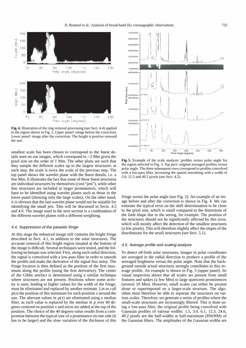
Fig. 4. Illustration of the ring removal processing (see Sect. 4.4) appliedto the region shown in Fig. 3. Upper panel: image before the correction.Lower panel: image after the correction. The height is positive outwardthe sun.

smallest scale has been chosen to correspond to the finest de-tails seen on our images, which correspond to ∼2 Mm given thepixel size on the order of 1 Mm. The other plans are such thatthey sample the different scales up to the largest structures: ateach step, the scale is twice the scale of the previous step. Thetop panel shows the wavelet plane with the finest details, i.e. afew Mm. It illustrates the fact that some of these finest structuresare individual structures by themselves (cool “jets”), while otherfine structures are included in larger prominences, which willhave to be identified using wavelet planes such as those in thelower panel (showing only the large scales). On the other hand,it is obvious that the last wavelet plane would not be suitable foridentifying the small jets. This will be discussed in Sects. 4.5and 4.6. The image used in the next section is a combination ofthe different wavelet planes with a different weighting.

4.4. Suppression of the parasitic fringe

At this stage the enhanced image still contains the bright fringedescribed in Sect. 4.1, in addition to the solar structures. Theaccurate removal of this bright region situated at the bottom ofthe image is difficult. Several techniques were tested, and the fol-lowing technique was selected. First, along each radial direction,the signal is convolved with a low-pass filter in order to smooththe profile and make the derivative of the signal less noisy. Thefringe location is then defined as the position of the first max-imum along the profile (using the first derivative). The centerof the Gibbs artefact is determined using a similar techniquewhere structures are not present. Positions where some activ-ity is seen, leading to higher values for the width of the fringe,must be eliminated and replaced by another estimate. Let us callp(x) the position of this minimum for each position x around thesun. The aberrant values in p(x) are eliminated using a medianfilter, as each value is replaced by the median in p over 40 de-grees centered on position x and zeros are added at the top of theposition. The choice of the 40 degrees value results from a com-promise between the typical size of a prominence on one side (ithas to be larger) and the slow variation of the thickness of this

Fig. 5. Example of the scale analysis: profiles versus polar angle forthe region selected in Fig. 3. Top part: original averaged profiles versuspolar angle. The three subsequent rows correspond to profiles convolvedwith a low-pass filter, increasing the spatial smoothing with a width of3.0, 12.3 and 49.2 pixels (see Sect. 4.5).

fringe versus the polar angle (see Fig. 2). An example of an im-age before and after the correction is shown in Fig. 4. We canestimate the typical error on the shift determination to be closeto the pixel size, which is small compared to the distortions ofthe limb shape due to the seeing, for example. The position ofthe structures should not be significantly affected by this error,which will mostly affect the detection of the smallest structures(a few pixels). This will therefore slightly affect the slopes of thedistributions for the small structures (see Sect. 5.1).

4.5. Average profile and scaling analysis

To detect off-limb solar structures, images in polar coordinatesare averaged in the radial direction to produce a profile of theaveraged brightness versus the polar angle. Note that the back-ground outside actual structures strongly contributes to this av-erage profile. An example is shown in Fig. 5 (upper panel). Itsvisual inspection shows that all scales are present from smallfeatures and spikes (a few Mm) to large quiescent prominences(several 10 Mm). However, small scales can either be presentalone or superimposed on a larger-scale structure. The algo-rithm must therefore be able to separate the structures on var-ious scales. Therefore, we generate a series of profiles where thesmall-scale structures are increasingly filtered. This is done us-ing a low-pass filter, the original profile being convolved withGaussian profiles of various widths: 1.5, 3.0, 6.1, 12.3, 24.6,49.2 pixels are the half-widths at half-maximum (HWHM) ofthe Gaussian filters. The amplitudes of the Gaussian widths are

736 D. Romeuf et al.: Analysis of broad-band Hα coronagraphic observations

chosen to cover the range of scales of the structures we haveto identify (see in particular Fig. 3), from small structures (aHWHM of 1.5 pixels corresponds to a width of about 2 Mm)to large structures (49.2 pixels corresponds to a width of about120 Mm).

An example of the processing is shown in Fig. 5. For eachprofile, the detection of structures is performed by detecting theprofile maximum, derived from the first derivatives, and the lo-cation of their inflexion points, derived from the second deriva-tives. Note that in the case of very large eruption events, we mustvisually impose the position. This second step is important forstudying evolution, such as the total brightness in the case ofa large prominence leading to a CME. At this stage, we obtainfor each profile 3 values of polar angles determining a struc-ture: the center position and the upper and lower limit positions.A fourth quantity is also computed: we call it the “strength”of the detected structure. It is the sum of the absolute valuesof the derivative over the entire structure inside the upper andlower limits. This quantity is useful for determining the thresh-old between background values and actual solar structures. Sucha threshold is experimentally defined for each spatial smooth-ing, as we visually checked on a small data set that we have noteliminated actual structures. Structures whose strengths are be-low the threshold are eliminated to avoid any false detection.The choice of the threshold has been made in a conservativeway, as another algorithm will be applied in Sect. 4.8 to the dailytime series in order to eliminate structures that might appear onlyonce.

4.6. Pyramidal analysis

Structures detected on various scales must be analyzed in orderto provide a single list of structures. Starting with the largestscale, a pyramidal analysis allows the elimination of the smallstructures located in a zone where a structure has already beendetected at the upper level. More specifically, we first considerthe structures defined on the largest scale. This identifies thelargest structures, the smallest ones being absent. Then, at thefollowing step (on a smaller scale), two categories of structuresare present: those that overlaps an already identified large struc-ture (therefore they are not to be considered) and those not over-lapping such structures (they are added to the list of structures).This is repeated until the smallest scale is reached. This is calledthe “extraction process” or simply the “extraction” further on. Alist of positions is derived from this analysis, and it provides thelocation of the structures described in Sect. 4.8.

4.7. Final products

To produce calibrated images in Cartesian coordinates and toprecisely estimate the intensities of the structures, the originalimages (obtained at the end of Sect. 4.1) are normalized to thesame standard. After properly subtracting the background, thedata is made available at BASS2000. An example is shown inFig. 6, where the bright fringe and the background were sub-tracted. In addition, the average activity level and its standarddeviation (showing the temporal variability of the activity level)over a day are computed in order to use this as a selection cri-terion in database requests. These images are used to extract F s,the light flux integrated over the whole structure, by summingthe intensities of each pixel between the two limits determiningthe structure (see Sect. 4.8).

Fig. 6. Upper panel: the background with the ring computed from theimage shown in Fig. 1 (see Sect. 4.7). Lower panel: the cleaned imageobtained after applying the background plus ring correction.

4.8. Structure parameters

In addition to the positions of each detected structure (lower andupper limits P1 and P2, and central positions Pc), several param-eters are computed using the images in polar coordinates, aftersuppression of the parasitic fringe:

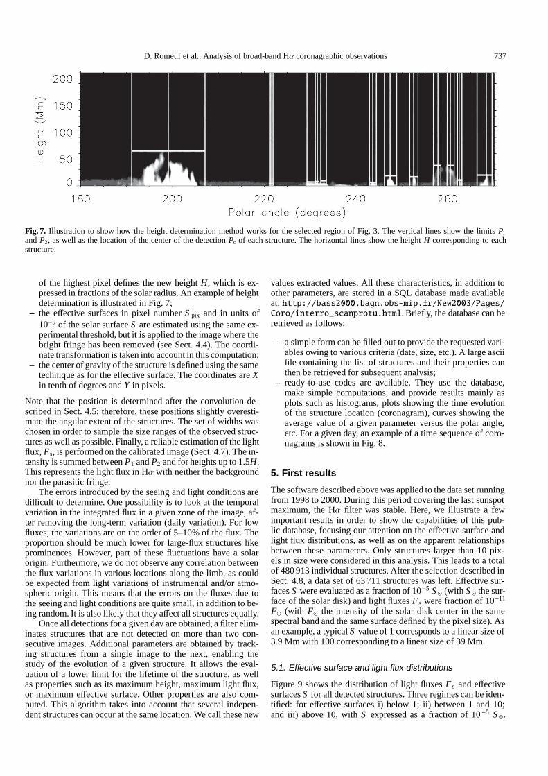
– the height H determined in two steps. First, a fast algorithmprovides an estimation by using the radial profile averagedbetween P1 and P2. Starting from the maximum of the inten-sity profile, the height where the profile reaches 10% of themaximum intensity gives a first estimate, H0. This value isarbitrary in some cases when a prominence is very complexand presents fine structure in the radial direction. A thresh-old is therefore experimentally defined in order to extract thepixels belonging to the structure. To eliminate possible con-tamination from the parasitic fringes occurring far from thelimb, only pixels below 2H0 are considered. The position

D. Romeuf et al.: Analysis of broad-band Hα coronagraphic observations 737

Fig. 7. Illustration to show how the height determination method works for the selected region of Fig. 3. The vertical lines show the limits P1

and P2, as well as the location of the center of the detection Pc of each structure. The horizontal lines show the height H corresponding to eachstructure.

of the highest pixel defines the new height H, which is ex-pressed in fractions of the solar radius. An example of heightdetermination is illustrated in Fig. 7;

– the effective surfaces in pixel number S pix and in units of10−5 of the solar surface S are estimated using the same ex-perimental threshold, but it is applied to the image where thebright fringe has been removed (see Sect. 4.4). The coordi-nate transformation is taken into account in this computation;

– the center of gravity of the structure is defined using the sametechnique as for the effective surface. The coordinates are Xin tenth of degrees and Y in pixels.

Note that the position is determined after the convolution de-scribed in Sect. 4.5; therefore, these positions slightly overesti-mate the angular extent of the structures. The set of widths waschosen in order to sample the size ranges of the observed struc-tures as well as possible. Finally, a reliable estimation of the lightflux, Fs, is performed on the calibrated image (Sect. 4.7). The in-tensity is summed between P1 and P2 and for heights up to 1.5H.This represents the light flux in Hα with neither the backgroundnor the parasitic fringe.

The errors introduced by the seeing and light conditions aredifficult to determine. One possibility is to look at the temporalvariation in the integrated flux in a given zone of the image, af-ter removing the long-term variation (daily variation). For lowfluxes, the variations are on the order of 5–10% of the flux. Theproportion should be much lower for large-flux structures likeprominences. However, part of these fluctuations have a solarorigin. Furthermore, we do not observe any correlation betweenthe flux variations in various locations along the limb, as couldbe expected from light variations of instrumental and/or atmo-spheric origin. This means that the errors on the fluxes due tothe seeing and light conditions are quite small, in addition to be-ing random. It is also likely that they affect all structures equally.

Once all detections for a given day are obtained, a filter elim-inates structures that are not detected on more than two con-secutive images. Additional parameters are obtained by track-ing structures from a single image to the next, enabling thestudy of the evolution of a given structure. It allows the eval-uation of a lower limit for the lifetime of the structure, as wellas properties such as its maximum height, maximum light flux,or maximum effective surface. Other properties are also com-puted. This algorithm takes into account that several indepen-dent structures can occur at the same location. We call these new

values extracted values. All these characteristics, in addition toother parameters, are stored in a SQL database made availableat: http://bass2000.bagn.obs-mip.fr/New2003/Pages/Coro/interro_scanprotu.html. Briefly, the database can beretrieved as follows:

– a simple form can be filled out to provide the requested vari-ables owing to various criteria (date, size, etc.). A large asciifile containing the list of structures and their properties canthen be retrieved for subsequent analysis;

– ready-to-use codes are available. They use the database,make simple computations, and provide results mainly asplots such as histograms, plots showing the time evolutionof the structure location (coronagram), curves showing theaverage value of a given parameter versus the polar angle,etc. For a given day, an example of a time sequence of coro-nagrams is shown in Fig. 8.

5. First results

The software described above was applied to the data set runningfrom 1998 to 2000. During this period covering the last sunspotmaximum, the Hα filter was stable. Here, we illustrate a fewimportant results in order to show the capabilities of this pub-lic database, focusing our attention on the effective surface andlight flux distributions, as well as on the apparent relationshipsbetween these parameters. Only structures larger than 10 pix-els in size were considered in this analysis. This leads to a totalof 480 913 individual structures. After the selection described inSect. 4.8, a data set of 63 711 structures was left. Effective sur-faces S were evaluated as a fraction of 10−5 S � (with S � the sur-face of the solar disk) and light fluxes F s were fraction of 10−11

F� (with F� the intensity of the solar disk center in the samespectral band and the same surface defined by the pixel size). Asan example, a typical S value of 1 corresponds to a linear size of3.9 Mm with 100 corresponding to a linear size of 39 Mm.

5.1. Effective surface and light flux distributions

Figure 9 shows the distribution of light fluxes F s and effectivesurfaces S for all detected structures. Three regimes can be iden-tified: for effective surfaces i) below 1; ii) between 1 and 10;and iii) above 10, with S expressed as a fraction of 10−5 S �.

738 D. Romeuf et al.: Analysis of broad-band Hα coronagraphic observations

Fig. 8. “Coronagrams” to show the time variations in the location of the detected structures for a continuous typical observing sequence from 6:10to 14:50 UT, taken on Aug. 2, 2000. The diagram shows all the recorded detections. Solar latitudes are shown along the vertical axis and the timeruns along the horizontal axis. The structures are selected using the filtering process described on Sect. 4.8. For this day a “coherence” of the largeprominence around the polar angle 48 degrees has been imposed (see Sect. 4.5).

For example, a small cool “jet”, such as those observed in theright part of Fig. 3 (between polar angles 90 and 110 ◦), cor-responds to an effective surface S on the order of 10 to 20.Similarly three regimes can be seen in the flux distribution.Distributions are also shown for the values after the “extrac-tions”. In this case, the fluxes and effective surfaces correspondto the maximum value over the day and therefore each structureis counted only once a day.

Different regimes can also be observed there, although theyare shifted slightly toward lower values. In the case of the distri-bution of effective surfaces S after selection (bottom of Fig. 9),we observe a power law for S in the range 0.2–30 and anotherpower law, much steeper, for S larger than ∼30, i.e. structuresdefinitely larger than jets. This could be due to the fact that theyare related to active regions rather than to the chromospheric net-work, as is the case for the smallest structures.

5.2. Relationships between structure parameters

Figure 10 shows the relationships between effective surfaces Sand fluxes Fs on a log-log scale. The relationship is found tobe approximately linear over almost three orders of magnitudes.It corresponds to a power law with a slope of 5/4. For largerstructures (i.e. for S larger than ∼60), the flux is smaller thanexpected from the linear fit. When looking into more details,there seems in fact to be two regimes in the linear domain, withtwo distinct slopes below an effective surface of 1 and aboveit. Below effective surfaces of 1, the slope is 1.108 ± 0.003 forall structures (0.999 ± 0.007 for the maximum values after the“extractions”), and it becomes 1.312 ± 0.001 (1.362 ± 0.007 forthe maximum values after the “extractions”) for S larger than 1.The slope is in general larger than 1, showing that in the lin-ear regime, larger structures have a larger flux per square pixelthan smaller ones. The exception is for small structures, witha slope consistent with 1, indicating a constant flux per square

D. Romeuf et al.: Analysis of broad-band Hα coronagraphic observations 739

Fig. 9. Upper panel: distribution of light fluxes Fs for all structures(solid lines) and the maximum light flux per structure after the selec-tion (dashed line), with Fs expressed as a fraction of 10−11 F� , duringthe period 1998–2000. Lower panel: distribution in effective surface Sfor all structures (solid lines) and the maximum total light flux per struc-ture after the selection (dashed line), with S expressed as a fraction of10−5 S �.

pixel for S up to 1. For large structures, the slope is significantlylarger after the “extractions”, showing that these parameters aremore pronounced when considering only the maximum duringthe lifetimes of the structures. This suggests different evolutionsfor the structures depending on their size and a possible influenceof the optical thickness on prominence elements. It could also beinteresting to look further at the relationship with the level of ac-tivity of the analyzed prominences, with their latitudes, etc. Weleave this research for a forthcoming paper. Finally, Fig. 10 alsoshows the variations with size of the rms dispersion of Log(F s)in each size bin. It shows that the dispersion is much larger forsmall structures, as can also be seen on the 2D distribution show-ing the number of structures versus S and F s. It is interesting tonotice that for small structures, the total extension of F s valuesfor a given size can reach 4 orders of magnitude, including a longweak tail toward weak light fluxes, which can be seen at the topof Fig. 10.

5.3. Polar angle distribution

Figure 11 shows the distributions versus polar angle for var-ious categories of sizes. The top row shows the distributionsfor structures identified on all images (i.e. before the selection

Fig. 10. Upper panel: light flux Fs versus effective surface S after theselection (maximum values over the lifetime are used), with S ex-pressed as a fraction of 10−5 S � and Fs expressed as a fraction of10−11 F�, for the period 1998–2000. The levels correspond to 1 struc-ture (black), 10 (blue), 50 (purple), 100 (red), 500 (orange), and 800(yellow). Middle panel: light fluxes Fs versus the effective surface Safter averaging in boxes of constant size in Log(S ), for all structures(solid line) and after the extraction process (dashed line). The two dot-ted lines correspond to the linear fits over S in the range 0.1–1 and Slarger than 1. Lower panel: rms dispersion of Log(Fs) in each S bin, forall structures (solid line) and after the selection (dashed line).

described in Sect. 4.8). In this case, a given structure is countedas many times as it appears. On the other hand, the distributionsin the bottom row correspond to structures after the selection:this eliminates a few uncertain structures and, more important,a given structure is now counted only once per day. The differ-ences between the two approaches is not easy to interpret, but itis in part related to the respective lifetimes of each category ofstructures. We are concentrating our analysis on the distributionafter selection.

Let us first consider the smallest structures, with S smallerthan 1. We observe a large number of structures in the activity

740 D. Romeuf et al.: Analysis of broad-band Hα coronagraphic observations

Fig. 11. Distribution of the number of structures versus the polar angle (counted positive counter-clockwise from the North pole), for all structures(top) and after the extraction, see 4.8 (bottom) over the period 1998–2000, for various size range S : smaller than 1 × 10−5 S � (le f t), between1 × 10−5 S � and 1 × 10−5 S � (middle) and larger than 10 × 10−5 S � (right). The vertical dashed lines represent the solar South pole position, andthe dotted lines represent the equator. Note the N-S asymmetry especially strong in polar regions for S smaller than 10 × 10−5 S �.

belts, with a gap at the equator. A smaller gap is observed be-tween the activity belts and the poles, which is much more pro-nounced in the Northern hemisphere as there is a very strongasymmetry between the two poles (twice as many structuresat the Northern pole). The number of structures is also greaterclose to the poles than at lower latitudes. When consideringlarger structures, for S in the range 1–10, we observe a simi-lar pattern in the activity belt, with the same gap at the equa-tor. The gap poleward of the activity belts is quite pronounced,again with a definite asymmetry between the numbers of struc-tures at the poles. However, the number of structures is nowquite small, as the distribution is dominated by the activitybelts. Large structures (S larger than 10) follow a pattern closeto the structures in the 1–10 S range. In particular, they alsoshow strong peaks in the 70–80◦ latitude range (especially inthe Southern hemisphere), in addition to the activity belts andstrong gaps at the poles. However, the distributions show a largerdispersion.

The dominating features for all structures are therefore smallgaps in activity at the equator and just above the activity belt,as well as a strong asymmetry between hemispheres, especiallyclose to the poles. Very small features are definitely more presentat the poles, and they have their highest rate of occurence there.

The gap at intermediate latitudes could be related to the factthat it has been difficult to establish a connection between thehigh latitude branch of solar activity (observed in the corona andusing filaments as tracers) and the low latitude one (activity belt),as illustrated for example in Leroy & Noëns (1983). This is ofparticular interest to the solar dynamo theories as it providessome constraints on the behavior of the dynamo waves. TheNorth-South asymmetry may also be related to the dynamo ac-tion. The fact that it is more pronounced at high latitudes showsthat the different components of the solar cycle (here the low-latitude branch and the high-latitude one) do not behave in thesame way. We cannot go further because the data considered inthis paper cover just a part of the solar cycle. It is our objectiveto study the evolution of the North-South asymmetry of the dis-tribution of small structures during the whole solar cycle and itspossible relationship with the polar magnetic field reversal in aforthcoming paper.

6. Conclusion

Special software was developed to process the large data set ofcoronagraphic data collected since 1994 in daily surveys at thePic du Midi Observatory. This software allows the detection ofstructures over a wide range of sizes, from small spikes to large

D. Romeuf et al.: Analysis of broad-band Hα coronagraphic observations 741

prominences. The preliminary results indicate interesting prop-erties over this wide range of light fluxes, i.e. over almost eightorders of magnitude and over more than three orders of magni-tude in effective surfaces.

The distributions of fluxes and effective surfaces show threedifferent regimes. The variations in fluxes with structure size isclose to linear over three orders of magnitude, with two slightlydifferent slopes for structures below or above 1 (this thresholdcorresponds to a linear size of 3.9 Mm). The large amount ofsamples also allows the study of the latitude distribution for thedifferent categories of set and shows a well-structured organi-zation, as well as asymmetries between hemispheres, as alreadyobserved by Noëns & Wurmser (2000). This database can there-fore potentially be used to study the parameters of small-scalestructures in detail, such as their spatial distribution in latitude,their lifetime distribution, as well as the variation in their prop-erties over the solar activity cycle and the relationship with theclosest active regions, eruptions, etc., taking the difference be-tween the Northern and Southern hemisphere distributions intoaccount. In this context, we recall that prominences have disk-filament counterparts and, accordingly, they are good proxies ofmagnetic neutral sheets well inside the inner corona. This willbe the subject of future work.

The statistical study of large structures such as prominencesis then made possible, as it will be easy to follow their variationsin brightness and height, including those leading to CMEs. Inaddition, these observations can easily be used in comparison toother data, such as that obtained by EIT and SUMER on SOHOin EUV and by LASCO at a much higher altitude above thelimb. Finally, the tool developed in this work could be appliedto any other coronagraphic data in Hα and partly to other coron-agraphic data, including those obtained with externally occultedinstruments in space (see Koutchmy 1988). It will, of course,be extensively used to process the data from the new corona-graphic and chromospheric instruments currently being devel-oped for the corona at the Pic du Midi Observatory.

Acknowledgements. Living expenses of the large number of associated ob-servers (O.A.) and most of the new equipment were covered by FIDUCIAL.Observations are also supported by PNST of the CNRS and INSU,Observatoire Midi-Pyrénées, Laboratoire d’Astrophysique of OMP and Institutd’Astrophysique de Paris, CNRS, and UPMC. We thank the BASS2000 tech-nical staff, as well as the technical teams of the Pic du Midi Observatory, fortheir help. We thank C. Latouche for his permanent interest and confidence, G.Stellmacher for reviewing the manuscript, Th. Roudier for useful discussions,J.-M. Abbadie for help running Pic du Midi facilities for us, J.-C. Vial for hisinterest and the anonymous referee for meaningful suggestions that led to sub-stantial improvements in the paper.

References

Collin, B., & Nesme-Ribes, E. 1995, C. R. Acad. Sci. Paris, 321(IIb), 77Delannée, C., Koutchmy, S., Delaboudinière, J.-P., et al. 1998, in Solar jets and

coronal plumes, ESA SP-421, 129Dere, K. P., Bartoe, J. F., Brueckner, G. E., & Recely, F. 1989, ApJ, 95, L345Fitzgibbon A., Pilu, M., & Fisher, R. B. 1999, IEEE Transactions on pattern

analysis and machine intelligence, 21(5), 476Fuller, N., Aboudarham, J., & Bentley, R. D., 2005, Sol. Phys., 227, 61Innes, D. E., Inhester, B., Srivastava, N., et al. 1999, Sol. Phys., 186, 337Koutchmy, S. 1988, Space Sci. Rev., 47, 95Koutchmy, S., & Loucif, M. L. 1991, in Mechanism of chromospheric and coro-

nal heating, Heidelberg Conf., ed. Ulmschneider, et al., 152Leroy, J.-L. 1972, Sol. Phys., 25, 413Leroy, J.-L., & Noëns, J.-C. 1983, A&A, L1Loucif, M. L., Koutchmy, S., Stellmacher, G., et al. 1998, in Solar jets and coro-

nal plumes, ESA SP-421, 299Niot, J. M., & Noëns, J.-C. 1997, Sol. Phys., 173, 53Noëns, J.-C., & Wurmser, O. 2000, Ap&SS, 273, 17Noëns, J.-C., Balestat, M.-F., Jimenez, R., et al. 2004, in Multi-Wavelength

Investigations of Solar Activity, Saint-Petersburg 14-19 june 2004,(Cambridge University Press), IAU Symposium, 223, 291

Holschneider, M., & Tchamitchian, P. 1990, Les ondelettes en 1989, ed. P.GLemarié, (Springer Verlag), 102

Robbrecht, E., & Berghmans, D. 2004, A&A, 425, 1097Romeuf, D., Rochain, S., Jimenez, R., et al. 2004, Atelier PNST, 26–29 Jan.

2004, Autrans, Livre des résumés, 109Shensa, J. 1992, IEEE. Trans. Signal Process., 40(10), 2464Starck, J.-L., & Murtagh, F. 1994, A&A, 288, 342Zharkova, V. V., Ipson, S. S., Zharkov, S. I., et al. 2003, Sol. Phys., 214, 89