ASTROPHYSICAL HIGH-ENERGY PHENOMENA DETECTED IN THE EARTH’S IONOSPHERE 4th School on Cosmic Rays and Astrophysics – UFABC – Sto André – 28/08/2010 4th School on Cosmic Rays and Astrophysics – UFABC – Sto André – 28/08/2010 Jean-Pierre Raulin Jean-Pierre Raulin Centro de Radioastronomia e Astrofísica Mackenzie, Universidade Presbiteriana Mackenzie, Escola de Engenharia, São Paulo, SP, Brasil
Transcript
ASTROPHYSICAL HIGH-ENERGY PHENOMENA DETECTED IN THE EARTH’S
IONOSPHERE
4th School on Cosmic Rays and Astrophysics – UFABC – Sto André – 28/08/20104th School on Cosmic Rays and Astrophysics – UFABC – Sto André – 28/08/2010
Jean-Pierre RaulinJean-Pierre Raulin
Centro de Radioastronomia e Astrofísica Mackenzie, Universidade Presbiteriana Mackenzie, Escola de Engenharia, São Paulo, SP, Brasil
Scientific Research at CRAAM/EE/UPM
SOLAR PHYSICS
IONOSPHERIC PHYSICS
GALACTIC AND EXTRAGALACTIC RADIO ASTROPHYSICS
SPACE GEODESICS
SOLAR-TERRESTRIAL RELATIONSHIP
ROEN
SST
ROI
COMTE. FERRAZ
SAVNET
CARPET + EFM 100
4th School on Cosmic Rays and Astrophysics – UFABC – Sto André – 28/08/2010
SST
Photosphere
H = 500 km ; T ~ 6000 K
Few Gauss < B < ~ 2500 G
4th School on Cosmic Rays and Astrophysics – UFABC – Sto André – 28/08/2010
TRACE 171 Ang. << 1
>> 1 = Pgas/Pmag
Solar Flares
1032 erg in few sec. to few min.
1041 e-/s > 20 keV
Solar Flares
Eth few 10 MK
Ek few 10 MeV
Emec CMEs4th School on Cosmic Rays and Astrophysics – UFABC – Sto André – 28/08/2010
Few 104 km
4th School on Cosmic Rays and Astrophysics – UFABC – Sto André – 28/08/2010
Solar Flares
Solar Flares
JTVkNE Beth2110.6~
2
3
thgr EE
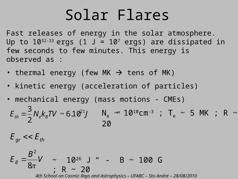
Fast releases of energy in the solar atmosphere. Up to 1032-33 ergs (1 J = 107 ergs) are dissipated in few seconds to few minutes. This energy is observed as :
• thermal energy (few MK tens of MK)
• kinetic energy (acceleration of particles)
• mechanical energy (mass motions - CMEs)
Ne ~ 1010cm-3 ; Te ~ 5 MK ; R ~ 20”
VB
EB 8
2
~ 1026 J - B ~ 100 G ; R ~ 20”
4th School on Cosmic Rays and Astrophysics – UFABC – Sto André – 28/08/2010
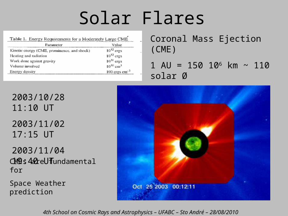
Coronal Mass Ejection (CME)
1 AU = 150 106 km ~ 110 solar Ø
Arrival time at 1 AU ~ 1.5 – 3 d
2003/10/28 11:10 UT
2003/11/02 17:15 UT
2003/11/04 19:40 UT
CMEs are fundamental for
Space Weather prediction
Solar Flares
4th School on Cosmic Rays and Astrophysics – UFABC – Sto André – 28/08/2010
CSR P4
CSR P1
ISR P1
ISR P4
ISR(?) pulses
Laboratory accelerators
4 November 2003 solar flare
4th School on Cosmic Rays and Astrophysics – UFABC – Sto André – 28/08/2010
The ionization of the neutral component of the Earth’s atmosphere is done through 2 processes
Photo-ionization (Chapman) and collision
4th School on Cosmic Rays and Astrophysics – UFABC – Sto André – 28/08/2010
The Earth Ionosphere
Inte
nsid
ade
da
Atm
osfe
ra N
eutr
a D
ecre
sce
Pic
os d
e D
ensi
dad
e O
casi
onad
as P
ela
Rad
iaçã
o S
olar
D en sid a d e E le trô n ica (cm -3 )
Alt
itud
e (k
m)
1 0 4 1 0 6
10 2
10 3
F 2
F 1
E
D
Pic
os d
e D
ensi
dad
e Io
nos
féri
ca
Inte
nsid
ade
da
Atm
osfe
ra N
eutr
a D
ecre
sce
Pic
os d
e D
ensi
dad
e O
casi
onad
as P
ela
Rad
iaçã
o S
olar
D en sid a d e E le trô n ica (cm -3 )
Alt
itud
e (k
m)
1 0 4 1 0 6
10 2
10 3
F 2
F 1
E
D
Pic
os d
e D
ensi
dad
e Io
nos
féri
ca
Inte
nsid
ade
da
Atm
osfe
ra N
eutr
a D
ecre
sce
Pic
os d
e D
ensi
dad
e O
casi
onad
as P
ela
Rad
iaçã
o S
olar
D en sid a d e E le trô n ica (cm -3 )
Alt
itud
e (k
m)
1 0 4 1 0 6
10 2
10 3
F 2
F 1
E
D
Pic
os d
e D
ensi
dad
e Io
nos
féri
ca
Inte
nsid
ade
da
Atm
osfe
ra N
eutr
a D
ecre
sce
Pic
os d
e D
ensi
dad
e O
casi
onad
as P
ela
Rad
iaçã
o S
olar
D en sid a d e E le trô n ica (cm -3 )
Alt
itud
e (k
m)
1 0 4 1 0 6
10 2
10 3
F 2
F 1
E
D
Pic
os d
e D
ensi
dad
e Io
nos
féri
ca
Inte
nsid
ade
da
Atm
osfe
ra N
eutr
a D
ecre
sce
Pic
os d
e D
ensi
dad
e O
casi
onad
as P
ela
Rad
iaçã
o S
olar
D en sid a d e E le trô n ica (cm -3 )
Alt
itud
e (k
m)
1 0 4 1 0 6
10 2
10 3
F 2
F 1
E
D
Pic
os d
e D
ensi
dad
e Io
nos
féri
ca
Inte
nsid
ade
da
Atm
osfe
ra N
eutr
a D
ecre
sce
Pic
os d
e D
ensi
dad
e O
casi
onad
as P
ela
Rad
iaçã
o S
olar
D en sid a d e E le trô n ica (cm -3 )
Alt
itud
e (k
m)
1 0 4 1 0 6
10 2
10 3
F 2
F 1
E
D
Pic
os d
e D
ensi
dad
e Io
nos
féri
ca
Inte
nsid
ade
da
Atm
osfe
ra N
eutr
a D
ecre
sce
Pic
os d
e D
ensi
dad
e O
casi
onad
as P
ela
Rad
iaçã
o S
olar
D en sid a d e E le trô n ica (cm -3 )
Alt
itud
e (k
m)
1 0 4 1 0 6
10 2
10 3
F 2
F 1
E
D
Pic
os d
e D
ensi
dad
e Io
nos
féri
ca
Inte
nsid
ade
da
Atm
osfe
ra N
eutr
a D
ecre
sce
Pic
os d
e D
ensi
dad
e O
casi
onad
as P
ela
Rad
iaçã
o S
olar
D en sid a d e E le trô n ica (cm -3 )
Alt
itud
e (k
m)
1 0 4 1 0 6
10 2
10 3
F 2
F 1
E
D
Pic
os d
e D
ensi
dad
e Io
nos
féri
ca
Inte
nsid
ade
da
Atm
osfe
ra N
eutr
a D
ecre
sce
Pic
os d
e D
ensi
dad
e O
casi
onad
as P
ela
Rad
iaçã
o S
olar
D en sid a d e E le trô n ica (cm -3 )
Alt
itud
e (k
m)
1 0 4 1 0 6
10 2
10 3
F 2
F 1
E
D
Pic
os d
e D
ensi
dad
e Io
nos
féri
ca
Inte
nsid
ade
da
Atm
osfe
ra N
eutr
a D
ecre
sce
Pic
os d
e D
ensi
dad
e O
casi
onad
as P
ela
Rad
iaçã
o S
olar
D en sid a d e E le trô n ica (cm -3 )
Alt
itud
e (k
m)
1 0 4 1 0 6
10 2
10 3
F 2
F 1
E
D
Pic
os d
e D
ensi
dad
e Io
nos
féri
ca
Inte
nsid
ade
da
Atm
osfe
ra N
eutr
a D
ecre
sce
Pic
os d
e D
ensi
dad
e O
casi
onad
as P
ela
Rad
iaçã
o S
olar
D en sid a d e E le trô n ica (cm -3 )
Alt
itud
e (k
m)
1 0 4 1 0 6
10 2
10 3
F 2
F 1
E
D
Pic
os d
e D
ensi
dad
e Io
nos
féri
ca
Inte
nsid
ade
da
Atm
osfe
ra N
eutr
a D
ecre
sce
Pic
os d
e D
ensi
dad
e O
casi
onad
as P
ela
Rad
iaçã
o S
olar
D en sid a d e E le trô n ica (cm -3 )
Alt
itud
e (k
m)
1 0 4 1 0 6
10 2
10 3
F 2
F 1
E
D
Pic
os d
e D
ensi
dad
e Io
nos
féri
ca
Inte
nsid
ade
da
Atm
osfe
ra N
eutr
a D
ecre
sce
Pic
os d
e D
ensi
dad
e O
casi
onad
as P
ela
Rad
iaçã
o S
olar
D en sid a d e E le trô n ica (cm -3 )
Alt
itud
e (k
m)
1 0 4 1 0 6
10 2
10 3
F 2
F 1
E
D
Pic
os d
e D
ensi
dad
e Io
nos
féri
ca
Inte
nsid
ade
da
Atm
osfe
ra N
eutr
a D
ecre
sce
Pic
os d
e D
ensi
dad
e O
casi
onad
as P
ela
Rad
iaçã
o S
olar
D en sid a d e E le trô n ica (cm -3 )
Alt
itud
e (k
m)
1 0 4 1 0 6
10 2
10 3
F 2
F 1
E
D
Pic
os d
e D
ensi
dad
e Io
nos
féri
ca
Ionization due to solar radiation
70
100
400
1000
Height (km)
4th School on Cosmic Rays and Astrophysics – UFABC – Sto André – 28/08/2010
The Earth Ionosphere
cos
:
:
:
:
:
:
dhds
N
s
I
Q
n
Rate of e- - ion production (cm-3s-1)
Intensity of radiation (energy flux in eV/m2/s)
Line-of-sight path length
Zenith angle
Photon absorption cross-section (m2)
Density of neutral
Ground
Sun
h
s
4th School on Cosmic Rays and Astrophysics – UFABC – Sto André – 28/08/2010
The Earth Ionosphere
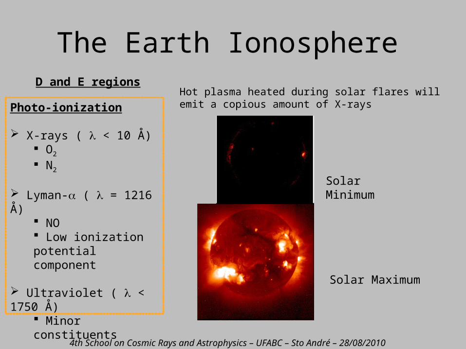
Hot plasma heated during solar flares will emit a copious amount of X-raysPhoto-ionization
X-rays ( < 10 Å) O2 N2
Lyman- ( = 1216 Å) NO Low ionization potential component
Ultraviolet ( < 1750 Å) Minor constituents
Solar Minimum
Solar Maximum
D and E regions
4th School on Cosmic Rays and Astrophysics – UFABC – Sto André – 28/08/2010
The Earth Ionosphere
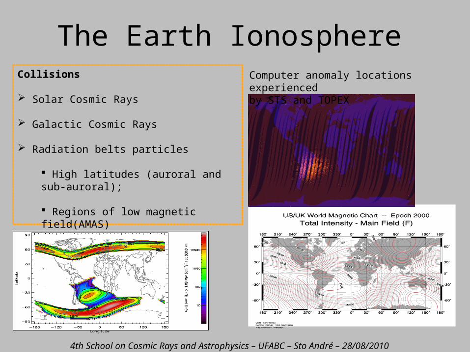
Collisions
Solar Cosmic Rays
Galactic Cosmic Rays
Radiation belts particles
High latitudes (auroral and sub-auroral);
Regions of low magnetic field(AMAS)
Computer anomaly locations experienced by STS and TOPEX
4th School on Cosmic Rays and Astrophysics – UFABC – Sto André – 28/08/2010
The Earth Ionosphere
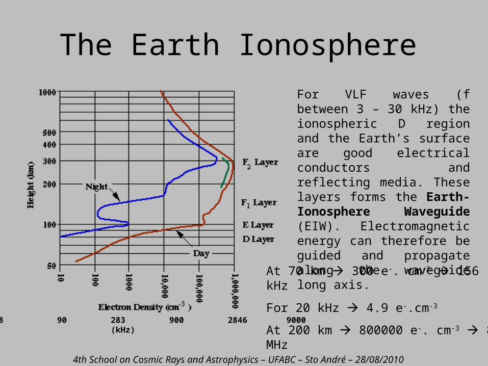
28 90 283 900 2846 9000 (kHz)
For VLF waves (f between 3 – 30 kHz) the ionospheric D region and the Earth’s surface are good electrical conductors and reflecting media. These layers forms the Earth-Ionosphere Waveguide (EIW). Electromagnetic energy can therefore be guided and propagate along the waveguide long axis.
4th School on Cosmic Rays and Astrophysics – UFABC – Sto André – 28/08/2010
The Earth Ionosphere
At 70 km 300 e-. cm-3 156 kHz
For 20 kHz 4.9 e-.cm-3
At 200 km 800000 e-. cm-3 8 MHz
XU
YT
2
sin 22 2
2
pX iZU 1
Z
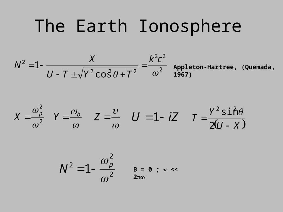
Appleton-Hartree, (Quemada, 1967)
bY
2
22
222
2
cos1
ck
TYTU
XN
2
22 1
pN B = 0 ; << 2
The Earth Ionosphere
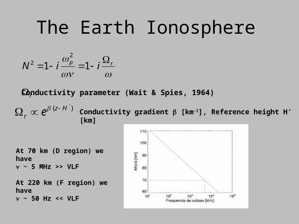
rp iiN
112
2
r Conductivity parameter (Wait & Spies, 1964)
)( 'Hzr e Conductivity gradient [km-1], Reference height H′ [km]
At 70 km (D region) we have ~ 5 MHz >> VLF
At 220 km (F region) we have ~ 50 Hz << VLF
The Earth Ionosphere
Increases of incoming X-ray fluxes during flares and increasing particle precipitations during geomagnetic storms produce ionization excesses and change of the electrical properties of the lower ionosphere D region. Then changing:
conductivity gradient [km-1] and reference height H′ [km]
Excesses of ionization can be monitored using the phase of long distance VLF propagating waves
r Conductivity parameter (Wait & Spies, 1964)
)( 'Hzr e Conductivity Gradient (sharpness) [km-1]
Reference height H′ [km]
4th School on Cosmic Rays and Astrophysics – UFABC – Sto André – 28/08/2010
The Earth Ionosphere
Wait 1950s-60s; Budden, 1961; Wait,1962
60 km
90 km
70 km
60 km
Δh
Solar flare
Ref. Height
Perturbed Ref. height
The lowering of H produces a change of the phase of the VLF wave. This change is measured by the VLF receiver, and can be expressed in terms of h. The change is proportional to the VLF path.
4th School on Cosmic Rays and Astrophysics – UFABC – Sto André – 28/08/2010
The Earth Ionosphere
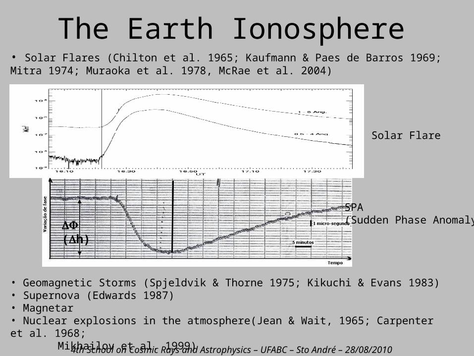
• Solar Flares (Chilton et al. 1965; Kaufmann & Paes de Barros 1969; Mitra 1974; Muraoka et al. 1978, McRae et al. 2004)
• Geomagnetic Storms (Spjeldvik & Thorne 1975; Kikuchi & Evans 1983)• Supernova (Edwards 1987)• Magnetar• Nuclear explosions in the atmosphere(Jean & Wait, 1965; Carpenter et al. 1968;
Mikhailov et al. 1999)
(h)
Solar Flare
SPA(Sudden Phase Anomaly)
4th School on Cosmic Rays and Astrophysics – UFABC – Sto André – 28/08/2010
The Earth Ionosphere
Raulin et al. 2006; Pacini & Raulin 2006
R > 0.95
~ 1 km
The low ionosphere is more sensitive during minimum of solar activity
Ionospheric indice for monitoring of the long-term solar radiation
McRae & Thomson 2000, 2004 showed that the quiescent (undisturbed) ionospheric D region reference height is higher during solar activity minimum periods by about ~ 1 km
For a given solar flare the lowering of the reference height is higher (by about 1 km) during solar minimum
hha
d
.
162
1360
3
2
t
dtdtRX
),(
4th School on Cosmic Rays and Astrophysics – UFABC – Sto André – 28/08/2010
The Earth Ionosphere Sensitivity
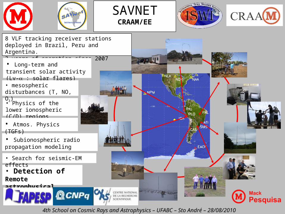
SAVNETCRAAM/EE
8 VLF tracking receiver stations deployed in Brazil, Peru and Argentina.3 years of operation since 2007
• Long-term and transient solar activity (Ly- ; solar flares)
• Physics of the lower ionospheric (C/D) regions
• mesospheric disturbances (T, NO, O3)
• Detection of Remote astrophysical objects
• Subionospheric radio propagation modeling
• Search for seismic-EM effects
4th School on Cosmic Rays and Astrophysics – UFABC – Sto André – 28/08/2010
• Atmos. Physics (TGFs)
Characteristics of the sensorsb ; A ; Ae
4th School on Cosmic Rays and Astrophysics – UFABC – Sto André – 28/08/2010
SAVNET: The basics
São Martinho da Serra, RS, 2007, May 1- 5
Punta Lobos, 2007, April 1- 8
Palmas, TO, 2007, May 21-26
Piura, 2007, June 5-11
CASLEO, 2007, Julio 1- 07
4th School on Cosmic Rays and Astrophysics – UFABC – Sto André – 28/08/2010
4th School on Cosmic Rays and Astrophysics – UFABC – Sto André – 28/08/2010
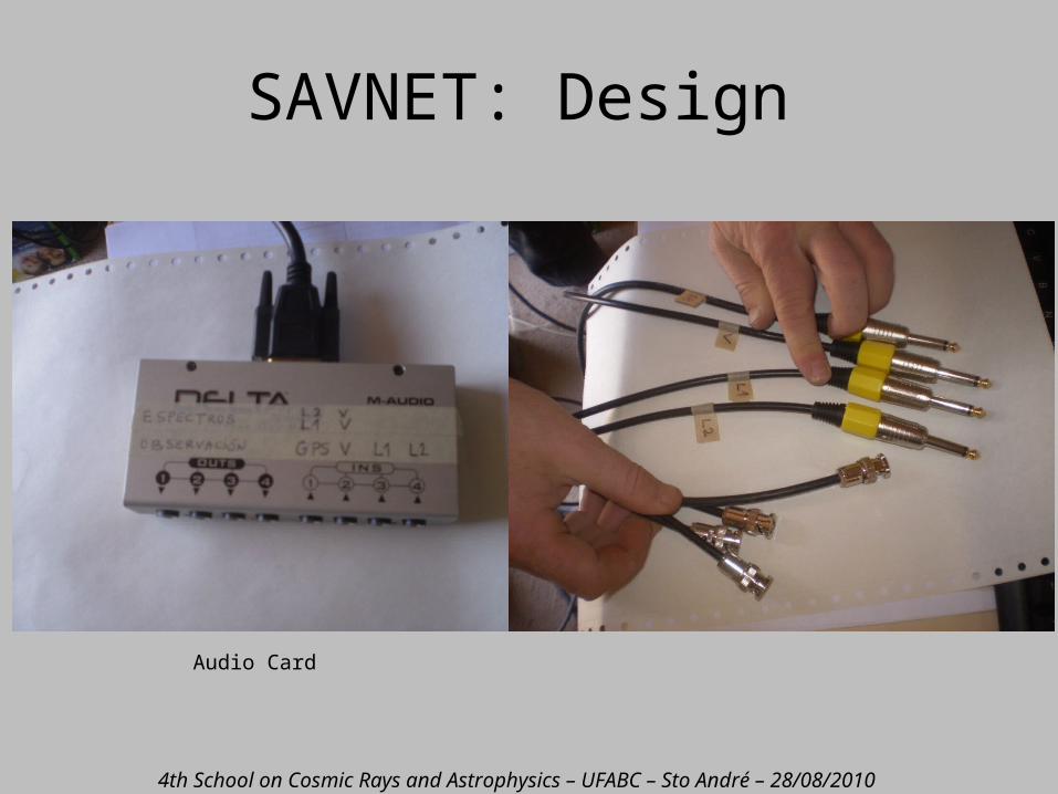
SAVNET: Design
Audio Card
4th School on Cosmic Rays and Astrophysics – UFABC – Sto André – 28/08/2010
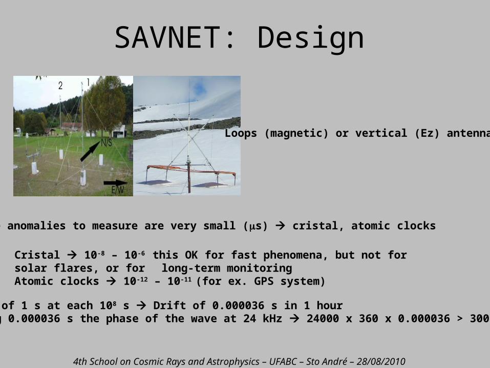
Loops (magnetic) or vertical (Ez) antennae
Phase anomalies to measure are very small (s) cristal, atomic clocks
Cristal 10-8 – 10-6 this OK for fast phenomena, but not for solar flares, or for long-term monitoring
Atomic clocks 10-12 – 10-11 (for ex. GPS system)
Drift of 1 s at each 108 s Drift of 0.000036 s in 1 hourDuring 0.000036 s the phase of the wave at 24 kHz 24000 x 360 x 0.000036 > 300 grados
SAVNET: Design
4th School on Cosmic Rays and Astrophysics – UFABC – Sto André – 28/08/2010
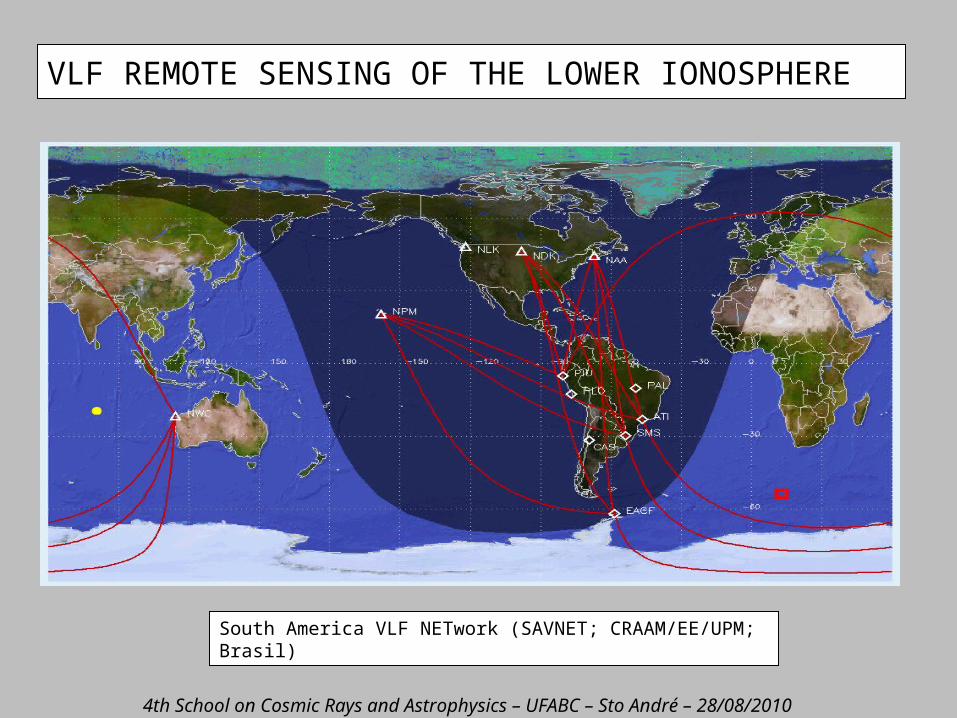
VLF REMOTE SENSING OF THE LOWER IONOSPHERE
South America VLF NETwork (SAVNET; CRAAM/EE/UPM; Brasil)
4th School on Cosmic Rays and Astrophysics – UFABC – Sto André – 28/08/2010
SENSITIVITY OF THE LOWER IONOSPHERE
4th School on Cosmic Rays and Astrophysics – UFABC – Sto André – 28/08/2010
(Raulin et al. 2010)
SENSITIVITY OF THE LOWER IONOSPHERE
4th School on Cosmic Rays and Astrophysics – UFABC – Sto André – 28/08/2010
(Raulin et al. 2010)
SENSITIVITY OF THE LOWER IONOSPHERE
4th School on Cosmic Rays and Astrophysics – UFABC – Sto André – 28/08/2010
Baker et al. 2004: Period of strong geomagnetic disturbances (Out-
Dez/2003): sucessive intense solar events with particles, shock waves
and CMEs
Important changes of Van Allen
radiation belts and intense precipitation of electrons from
these regions.
(Pacini, 2006)
GRBs and SGRs FLARES
• Soft Gamma-ray repeaters repeat sporadically from the same source (SNRs, AXPs), while Gamma-Ray Bursts have never been verified to come more than once from the same spot in the sky
• GRB are numerous while we know about 6 SGRs sources
• SGR are softer than GRB (less mean energy per photon)
• photon flux is generally higher for SGR
• SGR outbursts occur in group
• duration ranges from < 1 s to few minutes in average
• SGRs do produce some spectacular giant flares (3 known in 30 years)
• SGRs more probably originate in Magnetars (rotating neutron stars with B ~ 1015 G)
Observing and instrumental limitations:
• saturation during giant flares (problems to recover photon spectra)
• off-pointing (problems to recover photon spectra)
• Earth occultation (no observations)
4th School on Cosmic Rays and Astrophysics – UFABC – Sto André – 28/08/2010
SENSITIVITY OF THE LOWER IONOSPHERE
• The daytime sensitivity of the low ionospheric plasma has been estimated for daytime conditions, using solar flares as external forcing (Pacini & Raulin, 2006; Raulin et al. 2010)
- Minimum peak power detected at Earth orbit for [1.5 – 24 keV] photons : 2.7 10-4 erg/cm2/s (solar min.) and 10-3 erg/cm2/s (solar max.)
- Fluence > 14 keV, for 10 min. accumulated times:~ 10-7 erg/cm2 (solar min.) and few 10-7 erg/cm2 (solar max.)
• The nighttime sensitivity has been estimated to 10 times less than that during daytime (Tanaka, Raulin, Bertoni et al. 2010).
Therefore we do expect the VLF technique to detect intermediate-to-low SGRs and GRBs outbursts.
4th School on Cosmic Rays and Astrophysics – UFABC – Sto André – 28/08/2010
So far (30 years) , we know of 3 giant flares from SGRs. The most spectacular event occurred on 2004, December 27 at about 21:30 UT, from SGR 1806-20:
• estimated distance 15 kpc
• main peak (0.2 s) : rise < 1 ms, decay < 65 ms
• periodic tail (400 s), P ~ 7.56 s
• main peak satured all onboard -ray sensors
• Emain peak ~ total energy released by the Sun in
250 .103 years ~ 1010 times E (largest solar flares)
• lowering of daytime ionosphere ~ 10 km
• Magnetar, B ~ 1015 G
GIANT SGRs FLARES
RHESSI
4th School on Cosmic Rays and Astrophysics – UFABC – Sto André – 28/08/2010
VLF propagation path from NPM transmitter (Hawaii) to ATI observing station (São Paulo, Brazil). Also shown are the locations of other four VLF transmitters (NLK, NDK, NAA, and NAU). Shaded hemisphere indicates the night side part of the Earth at 06:48 UT, when the largest burst occurred. The part of the Earth illuminated by -rays at 6:48 UT is also drawn by dashed area. Although not shown, bursts were also detected by other SAVNET bases at Palmas, TO (PAL), São Martinho da Serra, RS (SMS), and Piura, Peru (PIU).
22-Jan. 2009, 0648 UT, larger burst
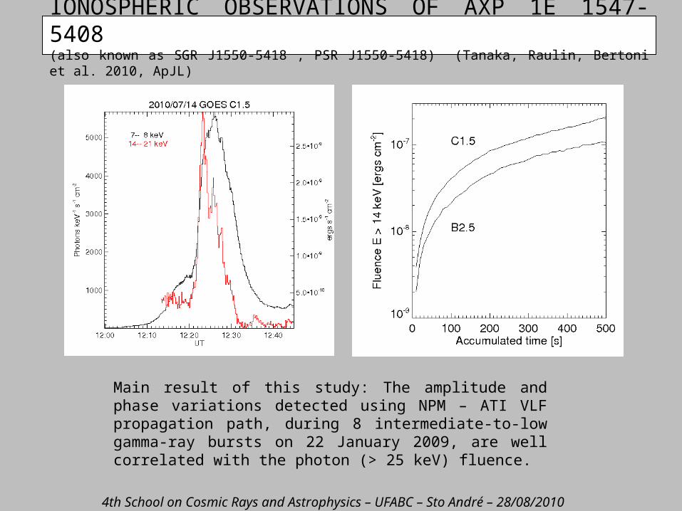
IONOSPHERIC OBSERVATIONS OF AXP 1E 1547-5408(also known as SGR J1550-5418 , PSR J1550-5418) (Tanaka, Raulin, Bertoni et al. 2010, ApJL)
4th School on Cosmic Rays and Astrophysics – UFABC – Sto André – 28/08/2010
IONOSPHERIC OBSERVATIONS OF AXP 1E 1547-5408(also known as SGR J1550-5418 , PSR J1550-5418) (Tanaka, Raulin, Bertoni et al. 2010, ApJL)
Over 100 -ray bursts were observed in the (South America) night of 22 January, 2009. Amplitude and phase variations of a VLF signal from NPM transmitter (21.4 kHz) are shown, which were observed at ATI from 04:00 UT to 10:00 UT. Lower figures are background-subtracted blown-ups at time ranges during which short repeated SGR bursts were detected.
22-Jan. 2009 bursts
4th School on Cosmic Rays and Astrophysics – UFABC – Sto André – 28/08/2010
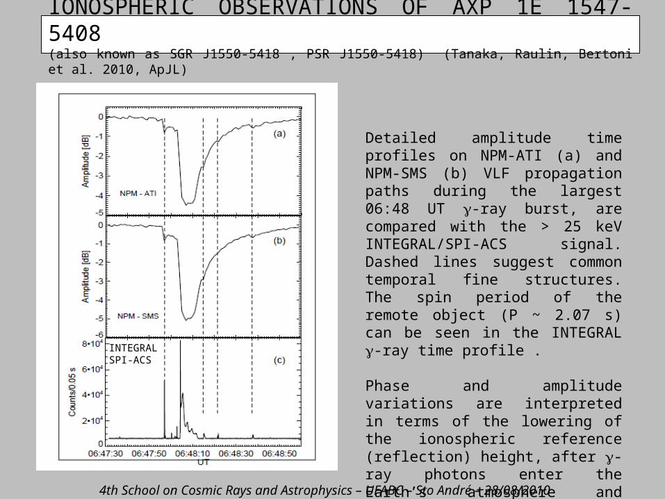
IONOSPHERIC OBSERVATIONS OF AXP 1E 1547-5408(also known as SGR J1550-5418 , PSR J1550-5418) (Tanaka, Raulin, Bertoni et al. 2010, ApJL)
Detailed amplitude time profiles on NPM-ATI (a) and NPM-SMS (b) VLF propagation paths during the largest 06:48 UT -ray burst, are compared with the > 25 keV INTEGRAL/SPI-ACS signal. Dashed lines suggest common temporal fine structures. The spin period of the remote object (P ~ 2.07 s) can be seen in the INTEGRAL -ray time profile .
Phase and amplitude variations are interpreted in terms of the lowering of the ionospheric reference (reflection) height, after -ray photons enter the Earth’s atmosphere and ionize the neutral component at and below ~ 85 km.
INTEGRALSPI-ACS
4th School on Cosmic Rays and Astrophysics – UFABC – Sto André – 28/08/2010
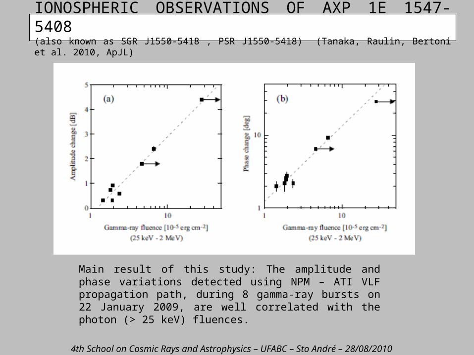
IONOSPHERIC OBSERVATIONS OF AXP 1E 1547-5408(also known as SGR J1550-5418 , PSR J1550-5418) (Tanaka, Raulin, Bertoni et al. 2010, ApJL)
Main result of this study: The amplitude and phase variations detected using NPM – ATI VLF propagation path, during 8 gamma-ray bursts on 22 January 2009, are well correlated with the photon (> 25 keV) fluences.
4th School on Cosmic Rays and Astrophysics – UFABC – Sto André – 28/08/2010
IONOSPHERIC OBSERVATIONS OF AXP 1E 1547-5408(also known as SGR J1550-5418 , PSR J1550-5418) (Tanaka, Raulin, Bertoni et al. 2010, ApJL)
Main result of this study: The amplitude and phase variations detected using NPM – ATI VLF propagation path, during 8 intermediate-to-low gamma-ray bursts on 22 January 2009, are well correlated with the photon (> 25 keV) fluence.
4th School on Cosmic Rays and Astrophysics – UFABC – Sto André – 28/08/2010
SUMMARY
The lower ionosphere plasma is a very sensitive medium to external forcing: radiation, energetic particle fluxes, atmospheric variability. It is therefore a unique laboratory to better track the Space Weather conditions and study the coupling with the upper and lower atmosphere.
The timescales involved give new insights on the monitoring of the long-term and transient solar activities, the episodic geomagnetic disturbances, and upper propagating phenomena in the neutral atmosphere.
We have detected, for the first time, ionospheric disturbances caused by intermediate-to-low short repeated gamma-ray bursts from a Magnetar. Amplitude and phase changes of Very Low Frequency propagating waves are well correlated with gamma-ray fluences. This can be understood in terms of the lowering of the ionospheric reflection height due to excesses of ionization at and below ~ 85 km.
While satellites in space cannot continuously observe the whole sky due to Earth occultation, the Earth’s ionosphere can monitor it without interruption. Very Low Frequency observations provide us with a new method, cheap and easy to implement, to monitor high energy transient phenomena of astrophysical importance.
Therefore, the Very Low Frequency diagnostic of high-energy astrophysical processes is, at least, a complementary information to space detections, and, sometimes, it may be the only way of recovering the incident photon spectrum at low energies.
4th School on Cosmic Rays and Astrophysics – UFABC – Sto André – 28/08/2010