Astudyof the

effects of waveson evaporation

fromfree water

surfaces

Research Report No. 18 • A WATER RESOURCES TECHNICAL PUBLICATION

Astudyof theeffects of waveson evaporationfromfree watersurfaces

prepared by Calvin C. Easterbrook,

Cornell Aeronautical Laboratory, Inc.,

for the Bureau of Reclamation

UNITED STATES DEPARTMENT OF THE INTERIOR

BUREAU OF RECLAMATION

As the Nation's principal conservation agency, the Department of theInterior has basic responsibilities jor water, fish, wildlife, mineral, land,park and recreational resources. Indian and Territorial affairs are othermajor concerns of America's "Department of Natural Resources."The Department works to assure the wisest choice in managing all ourresources so each will make its jull contribution to a better United States­now and in the juture.

First Printing: 1969

U.S. GOVERNMENT PRINTING OFFICE

WASHINGTON: 1969

For sale by the Superintendent of Documents, U.S. Government Printing Office, Washington, D.C.20402, or the Chief Engineer, Bureau of Reclamation, Attention 841, Denver Federal Center, Denver,Colo. 80225. Price 65 cents.

PREFACE

For several years, the Bureau of Reclamation hasconducted research in the use of monomolecularfilms (monolayers) of fatty alcohols and similar ma­terials placed on water surfaces to retard evaporation.The incentive for this research is to reduce the greatevaporation losses from large lakes and reservoirs inthe 17 western United States, estimated at morethan 14 million acre-feet annually, and at the sametime to improve the quality of the water in the lakesand reservoirs.

The Bureau's research program in evaporation re­duction is being carried out at selected field sites and inthe Bureau's Engineering and Research Center at Den­ver, as well as through contracts with educationalinstitutions, other government agencies, and com­mercial research organizations. Among these activ­ities is the investigation to determine the quantita­tive relationship between wave and air flow character­istics and the evaporation rate, and to increase under­standing of the microphysical processes that controlthe rate of mass transport across a water surface. Suchan investigation, described in this Research Report, isimportant because, as the author states, " ...waves

on a water surface have a significant effect on theevaporation rate from that surface".

The work described herein was carried out byCalvin C. Easterbrook of the Cornell AeronauticalLaboratory, Inc., of Cornell University at Buffalo,N. Y., under research contract No. 14-06-D-5764with the Bureau of Reclamation. The original reportwas given limited distribution under its designation,CAL Report No. RM-2151-P-l, dated April 15,1968. As Mr. Easterbrook's research work is of con­tinuing interest to researchers studying the use ofmonolayers, it is reprinted here as a Bureau of Rec­lamation Water Resources Technical Publication.

Included in this publication is an informativeabstract with a list of descriptors, or keywords, and"identifiers". The abstract was prepared as part ofthe Bureau of Reclamation's program of indexingand retrieving the literature of water resources de­velopment. The descriptors were selected from theThesaurus oj Descriptors, which is the Bureau's stand­ard for listing of keywords.

Other recent issues in the Water Resources Tech­nical Publications group are listed on the inside backcover of this report.

ACKNOWLEDGMENTS

I wish to express sincere appreciation for theassistance and cooperation given by Dr. BradfordBean, Mr. Ray McGavin, and several other membersof the Radio Meteorology Section, TroposphericTelecommunications Laboratory, of the Environ­mental Science Services Administration. Withoutthe meteorological data supplied by the ESSA group,the CAL study of wave-evaporation interaction atLake Hefner would not likely have been possible. Ialso wish to thank the many people from the Bureauof Reclamation for their continued interest in and

support of this work and for their willing assistanceduring the Lake Hefner field program.

This report has been approved by George E. Mc­Vehil, Head, Dynamic Meteorology Section, andRoland J. Pilie, Assistant Head, Applied PhysicsDepartment of the Cornell Aeronautical Laboratory,Inc.

CALVIN C. EASTERBROOK.

iii

CONTENTSPage

Preface_ ___________________________________________________________ iiiAcknowledgments_____ _____ __ __ __ __ __ __ __ __ __ __ __ __ __ __ __ __ __ __ __ __ _ iiiSummary__________________________________________________________ 1Introduction _______________________________________________________ 3

The wave tank evaporation experiments________________________________ 5Evaporation tank design and instrumentation _______________________ 5Development of evaporation tank theory___________________________ 7Results of the wave tank evaporation experiments ___________________ 10Investigation of evaporation controlling mechanisms_ _________ __ __ __ _ 12Conclusions ____________________________________________________ 21

The Lake Hefner evaporation study___________________________________ 22Instrumentation at Lake Hefner___________________________________ 22Data acquisition ________________________________________________ 24Processing and analysis of Lake Hefner data_ _______________________ 25

Comparison of the laboratory and field results_ __________________________ 33

Evaporation estimates and waves______________________________________ 35

Conclusions and recommendations_ ____________________________________ 39

References_________________________________________________________ 41

Appendix:

A. Bridge circuit used for thermistor temperature measurements in windtunnel________________________________________________________ 43

B. Solution of wave tank electrical analog____________________________ 45C. Design and construction details of the wave probe____________________ 47D. Basic data from the wave tank evaporation experiments _______________ 51E. Reduced Lake Hefner data________________________________________ 53

Abstract___________________________________________________________ 58

FIGURESNumber

1. Schematic diagram of evaporation tank_ ____________________________ 52. Evaporation tank in final stages of construction ______________________ 63. Wave generating assembly________________________________________ 64. High capacity fan installation_ ____________________________________ 6

v

Number

5. The return duct observed through fan blades _6. Beach trap modification _7. Electrical analog of evaporation experiment- _8. Normalized specific humidityas a function of time _9. Evaporation coefficient D in feet per second as a function of wind speed

and wave parameter HI T _

10. Evaporation coefficient as a function of wave parameter for constantwind speeds- _

11. Temperature and humidity as a function of time, experiment No. 108__12. Helium bubble stationary behind wave crest- _13. Bubble trajectories over surface with only wind-driven capillary waves

present _

14. Bubble trajectories over well-developed waves- _15. Smoke tracers over well-developed waves- _16. Smoke tracers over breaking waves- _17. Smoke bubble released from under water- _

18. Smoke tracers showing reverse flow of air near surface ahead of ap-proaching wave cresL _

19. Model of air flow over well-developed waves- _20. Map of Lake Hefner, Oklahoma City, Okla. _21. Basic wave probe configuration _22. Wave probe installation at Lake Hefner, 1966 _23. Wave probe installation at the Mid-lake tower, 1967 _24. Sample wave spectra, August 1966 _

25. Evaporation coefficient D as a function of wind speed, Mid-lake tower __26. Evaporation coefficient D as a function of wind speed, Intake tower _27. Total wave energy as a function of the 2-meter wind speed _28. Wave parameter HIT as a function of the 2-meter wind speed _29. Evaporation coefficient D as a function of the wave parameter HIT for

the 2-meter level at the Intake tower _

30. Contours of constant D as a function of wave parameter HIT and windspeed-Contours adjusted to fit the Lake Hefner results _

31. Mass transfer coefficient N as a function of wind speed - _- __32. Mass transfer coefficient N as a function of wind speed-Curve adjusted

to fit water budget data - - _- _- - - __

Page

679

10

11

131415

1616171819

2021232425262728293031

31

3437

38

vi

A-1. Schematic diagram of pulsed thermistor bridge _____________________ 43B-1. Electrical analog of evaporation experimenL _______________________ 45C-1. Block diagram of probe system ___________________________________ 47C-2. Schematic diagram of wave probe system_ __ __ __ ____ ____ __ __ __ __ __ _ 48C-3. Wave probe calibration curve____________________________________ 49C-4. Wave measuring probe__________________________________________ 50

SUMMARY

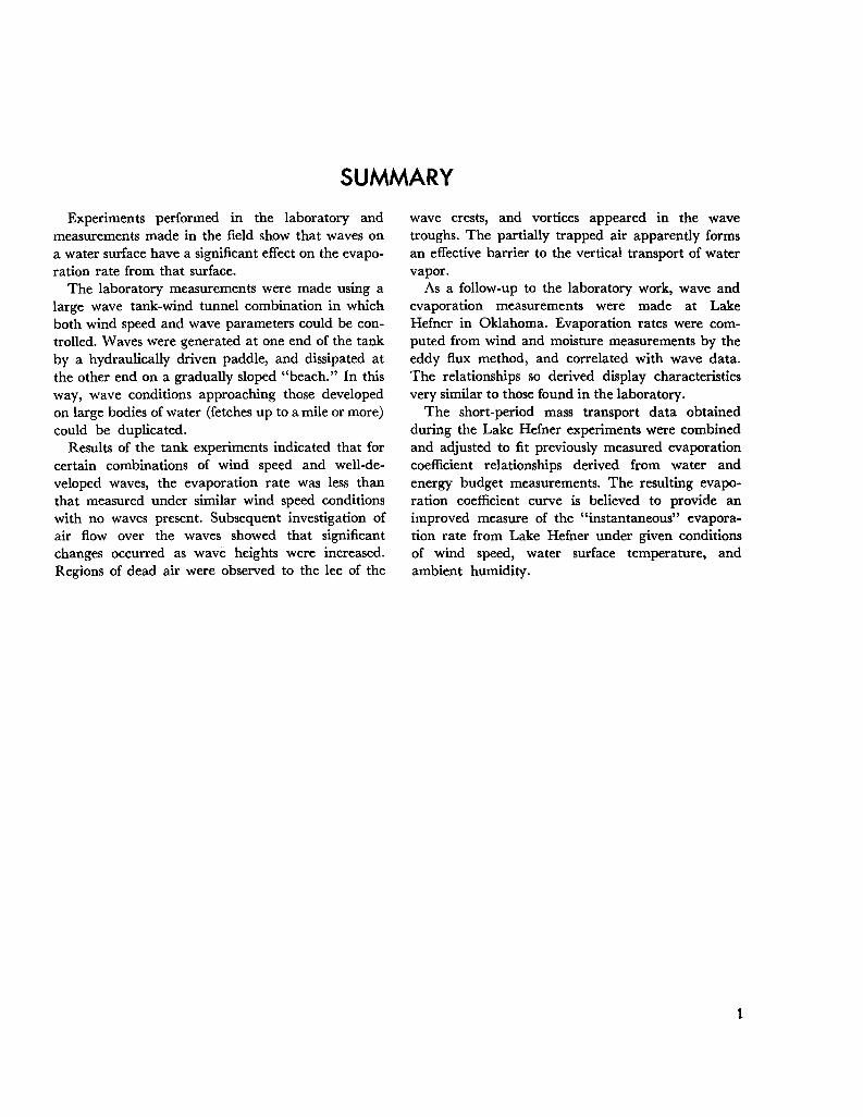
Experiments performed in the laboratory andmeasurements made in the field show that waves ona water surface have a significant effect on the evapo­ration rate from that surface.

The laboratory measurements were made using alarge wave tank-wind tunnel combination in whichboth wind speed and wave parameters could be con­trolled. Waves were generated at one end of the tankby a hydraulically driven paddle, and dissipated atthe other end on a gradually sloped "beach." In thisway, wave conditions approaching those developedon large bodies of water (fetches up to a mile or more)could be duplicated.

Results of the tank experiments indicated that forcertain combinations of wind speed and well-de­veloped waves, the evaporation rate was less thanthat measured under similar wind speed conditionswith no waves present. Subsequent investigation ofair flow over the waves showed that significantchanges occurred as wave heights were increased.Regions of dead air were observed to the lee of the

wave crests, and vortices appeared in the wavetroughs. The partially trapped air apparently formsan effective barrier to the vertical transport of watervapor.

As a follow-up to the laboratory work, wave andevaporation measurements were made at LakeHefner in Oklahoma. Evaporation rates were com­puted from wind and moisture measurements by theeddy flux method, and correlated with wave data.The relationships so derived display characteristicsvery similar to those found in the laboratory.

The short-period mass transport data obtainedduring the Lake Hefner experiments were combinedand adjusted to fit previously measured evaporationcoefficient relationships derived from water andenergy budget measurements. The resulting evapo­ration coefficient curve is believed to provide animproved measure of the "instantaneous" evapora­tion rate from Lake Hefner under given conditionsof wind speed, water surface temperature, andambient humidity.

1

INTRODUCTION

where E= evaporation rateVa = mean wind speed at level ae. = saturation vapor pressure at temperatUl e

of the water surfaceea = mean vapor pressure at level aN= constant.

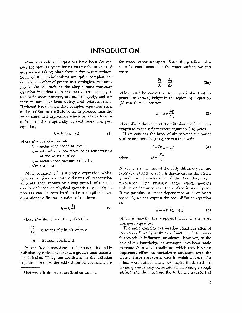
While equation (1) is a simple expression whichapparently gives accurate estimates of evaporationamounts when applied over long periods of time, itcan be defended on physical grounds as well. Equa­tion (1) can be considered to be a simplified one­dimensional diffusion equation of the form

Many methods and equations have been derivedover the past 100 years for estimating the amount ofevaporation taking place from a free water surface.Some of these relationships are quite complex, re­quiring a number of precise meteorological measure­ments. Others, such as the simple mass transportequation investigated in this study, require only afew basic measurements, are easy to apply, and forthese reasons have been widely used. Marciano andHarbeck l have shown that complex equations suchas that of Sutton are little better in practice than themuch simplified expressions which usually reduce toa form of the empirically derived mass transportequation,

(5)

(3)

(4)

(2a)aq ~q-=-az ~

~qE=Kw ­

~z

E=NV.(q,-q.)

KwD=­

z

E=D(q,-q.)

where

D, then, is a measure of the eddy diffusivity for thelayer (0 - z) and, as such, is dependent on the heightZ and the characteristics of the boundary layerturbulence. The primary factor which governsturbulence intensity near the surface is wind speed.If we postulate a linear dependence of D on windspeed V., we can express the eddy diffusion equationas

where Kw is the value of the diffusion coefficient ap­propriate to the height where equation (2a) holds.

If we consider the layer of air between the watersurface and some height Z, we can then write

which must be corf(,:ct at some particular (but ingeneral unknown) height in the region ~. Equation(2) can then be written

for water vapor transport. Since the gradient of qmust be continuous near the water surface, we canwrite

(1)

(2)aq

E=K­azwhere E= flux of q in the Z direction

aq d' f' d' .- = gra lent 0 q 10 lrectlOn ZazK = diffusion coefficient.

In the free atmosphere, it is known that eddydiffusion by turbulence is much greater than molecu­lar diffusion. Thus, the coefficient in the diffusionequation becomes the eddy diffusion coefficient Kw

1 References in this report are listed on page 41.

which is exactly the empirical form of the masstransport equation.

The more complex evaporation equations attemptto express D analytically as a function of the manyfactors which influence turbulence. However, to thebest of our knowledge, no attempts have been madeto relate D to wave conditions, which may have animportant effect on turbulence structure over thewater. There are several ways in which waves mightaffect evaporation. First, we might think that in­creasing waves may constitute an increasingly roughsurface and thus increase the turbulent transport of

3

water vapor. Also, the existence of bubbles, breakingon the wave crests, might constitute a significant de­crease in the surface resistance to mass flux, thus in­creasing evaporation. Associated with this lattermechanism is another which might be even more im­portant; that is, the creation of a vapor source aboveZ = 0 due to spray blown off breaking waves.

It is also possible to envision an effect opposite tothe first suggestion above: instead of waves makingthe surface aerodynamically more rough, just theopposite may be true. A suggestion along these lineshas been proposed by Stewart. Stewart presents ar­guments to show that traveling and developingwaves on a water surface may give rise to an or­ganized air flow pattern near the surface. This or­ganized flow, while being able to transport mo­mentum, would act as a barrier to heat and masstransport. A further argument related to the above issuggested by a postulate put forward by Phillips.Phillips found that waves develop most rapidly by aresonance mechanism which occurs when a compo­nent of the surface pressure distribution moves at thesame speed as the free surface wave with the samewave number. Phillips' results suggest that certaincombinations of wave conditions and wind speedmight favor the development of organized flow asdiscussed by Stewart.

Because of the many unknowns in the evaporationprocess and its relation to waves on the evaporatingsurface, Cornell Aeronautical Laboratory undertook

4

a combined laboratory and field study of waveeffects on evaporation for the Bureau of Reclamation.The study began in September 1965 and continuedthrough January 1968 under two extensions to theoriginal contract. The overall objectives of the workwere as follows:

1. Determine the quantitative relationship betweenwave characteristics, air flow characteristics, andevaporation rate.

2. Investigate the microphysical processes thatcontrol the rate of mass transport across the watersurface and the way in which these processes changewith wave activity.

3. Develop methods for applying laboratory re­sults to field situations.

4. Develop a general evaporation prediction tech­nique and formulate simple expressions that makeuse of data from routinely available observations toobtain an estimate of the evaporation loss from un­treated open water surfaces.

The work has progressed in two separate phases.Phase 1, completed in July 1966, consisted entirelyof laboratory measurements and was directed mainlytoward objectives 1 and 2. Phase 2 was a field studyof evaporation processes at Lake Hefner, and wasaimed at satisfying objectives 3 and 4. This documentis the final report under the contract and describesthe results of all work performed during the contractperiod.

THE WAVE TANK EVAPORATION EXPERIMENTS

The laboratory experiments described herein werecarried out in a wave tank, originally constructed atCAL for use in the study of water waves by Dopplerradar. The wave tank consists of a large open trough,40 feet long, 4 feet wide, and 3 feet deep with anelectrically driven paddle at one end of the tank. Thepaddle generates waves which travel down thetrough and are dissipated on a gently sloping "beach".

For the evaporation experiments the wave tankWas enclosed and a large fan was installed to circu­late air over the water surface. Instruments wereinstalled to make measurements of the moisture con­tent, temperature, and speed of the air moving overthe evaporating surface. Details of the evaporationexperiments are given below.

Evaporation Tank Design andInstrumentation

A diagram of the combination wave and evapora­tion tank is shown in figure 1. A return duct con­structed on top of the existing wave tank carries the

output air back to the input forming a closed recircu­lating system. A high capacity, variable speed faninstalled in the return duct provides the controlledwind speed along the evaporation section of the tank.The ports at the beach end of the structure permitthe system to be charged with dry air at the beginningof each experiment. Closing port C and openingports A and B allows dry air to be drawn in throughA while the tank is being purged of moist air throughB. Wave generation is accomplished in the tank witha motor driven paddle, as shown in figure 1. Theamplitude and frequency of the paddle excursioncan be controlled in the paddle drive system, thussetting the desired wave parameters. Details of thepaddle drive may be seen in figure 3. The evaporationtank in its final stages of construction is shown infigure 2.

During initial trial experiments with the completedtank it became apparent that the "beach" was in­troducing some undesirable effects. Waves whichwere stable down the main section of the tank beganbreaking on approaching the beach. Increasing the

0J DATA RECORDING STATIONS

CDVARIABLE

SPEEDPULLY

..EVAPORATION SECTION

.. BEACH TRAP ----:==-_--'111

•

INSTRUMENTSTATI ON 2

-_---..j

---

ijO FEET

•..---- 2.5 FEET

3 FEET----<-

WAVE GENERATINGPADDLE

INSTRUMENTSTATION 1

Figure I.-Schematic diagram of evaporation tank.

5

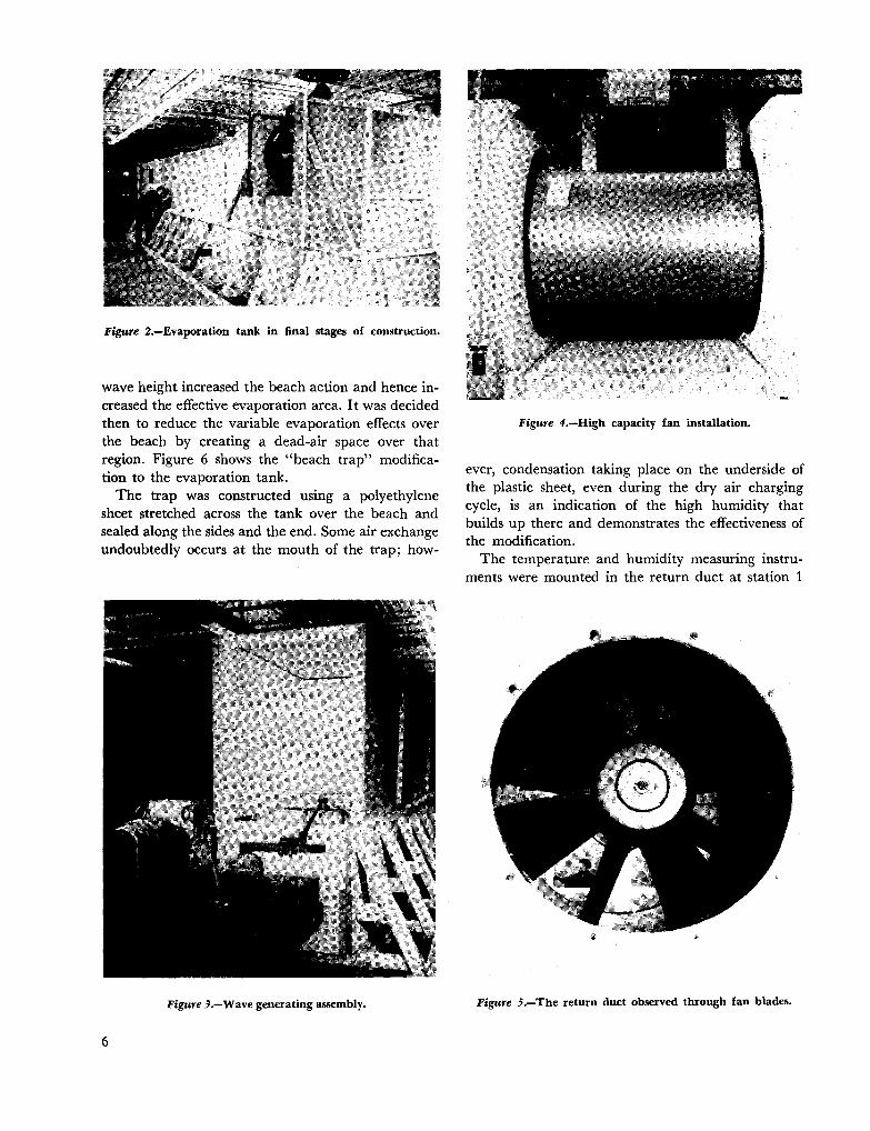
Figure 2.-Evaporation tank in final stages of construction.

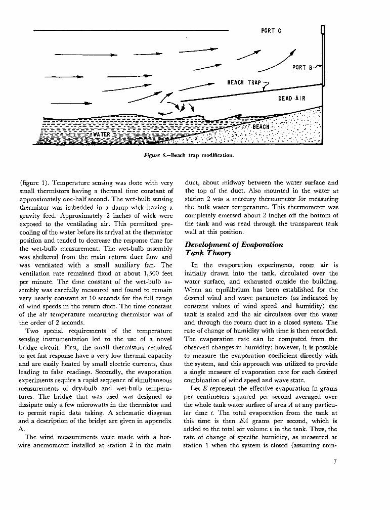
wave height increased the beach action and hence in­creased the effective evaporation area. It was decidedthen to reduce the variable evaporation effects overthe beach by creating a dead-air space over thatregion. Figure 6 shows the "beach trap" modifica­tion to the evaporation tank.

The trap was constructed using a polyethylenesheet stretched across the tank over the beach andsealed along the sides and the end. Some air exchangeundoubtedly occurs at the mouth of the trap; how-

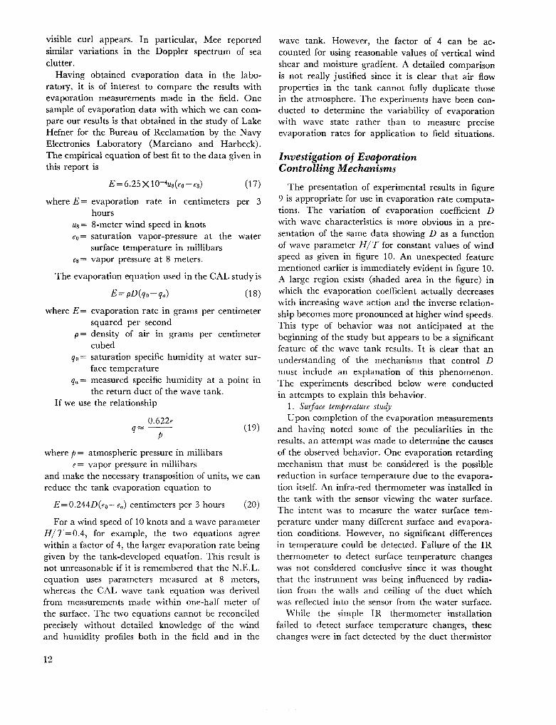
Figure J.-Wave generating assembly.

6

Figure 4.-High capacity fan installation.

ever, condensation taking place on the underside ofthe plastic sheet, even during the dry air chargingcycle, is an indication of the high humidity thatbuilds up there and demonstrates the effectiveness ofthe modification.

The temperature and humidity measuring instru­ments were mounted in the return duct at station 1

Figure 5.-The return duct observed through fan blades.

to - -----

Figure 6.-Beach trap modification.

PORT C

~~ORTB

(figure 1). Temperature sensing was done with verysmall thermistors having a thermal time constant ofapproximately one-half second. The wet-bulb sensingthermistor was imbedded in a damp wick having agravity feed. Approximately 2 inches of wick wereexposed to the ventilating air. This permitted pre­cooling of the water before its arrival at the thermistorposition and tended to decrease the response time forthe wet-bulb measurement. The wet-bulb assemblywas sheltered from the main return duct flow andwas ventilated with a small auxiliary fan. Theventilation rate remained fixed at about 1,500 feetper minute. The time constant of the wet-bulb as­sembly was carefully measured and found to remainvery nearly constant at 10 seconds for the full rangeof wind speeds in the return duct. The time constantof the air temperature measuring thermistor was ofthe order of 2 seconds.

Two special requirements of the temperaturesensing instrumentation led to the use of a novelbridge circuit. First, the small thermistors requiredto get fast response have a very low thermal capacityand are easily heated by small electric currents, thusleading to false readings. Secondly, the evaporationexperiments require a rapid sequence of simultaneousmeasurements of dry-bulb and wet-bulb tempera­tures. The bridge that was used was designed todissipate only a few microwatts in the thermistor andto permit rapid data taking. A schematic diagramand a description of the bridge are given in appendixA.

The wind measurements were made with a hot­wire anemometer installed at station 2 in the main

duct, about midway between the water surface andthe top of the duct. Also mounted in the water atstation 2 was a mercury thermometer for measuringthe bulk water temperature. This thermometer wascompletely emersed about 2 inches off the bottom ofthe tank and was read through the transparent tankwall at this position.

Development of EvaporationTank Theory

In the evaporation experiments, room air isinitially drawn into the tank, circulated over thewater surface, and exhausted outside the building.When an equilibrium has been established for thedesired wind and wave parameters (as indicated byconstant values of wind speed and humidity) thetank is sealed and the air circulates over the waterand through the return duct in a closed system. Therate of change of humidity with time is then recorded.The evaporation rate can be computed from theobserved changes in humidity; however, it is possibleto measure the evaporation coefficient directly withthe system, and this approach was utilized to providea single measure of evaporation rate for each desiredcombination of wind speed and wave state.

Let E represent the effective evaporation in gramsper centimeters squared per second averaged overthe whole tank water surface of area A at any particu­lar time t. The total evaporation from the tank atthis time is then EA grams per second, which isadded to the total air volume v in the tank. Thus, therate of change of specific humidity, as measured atstation 1 when the system is closed (assuming com-

7

and (10) and differentiate with respect to t, we ob­tain the differential equation

plete mixing in the return duct), is

dq AE-d = - grams per gram per second

t vp

(6)

V d2q dq--+D-=OA dt 2 dt

(11)

Equation (7) then permits a computation of evapora­tion rate from the slope of the measured q(t) curveif the air volume in the tank and the effective watersurface area are known.

Let us next consider the simple bulk aerodynamicevaporation equation

q=O for t=O

for the boundary conditions of our experiment, i.e.,

for t= IX)q=q.

vThe quantity DA is the time constant of the evapora-

q(t) =q. [1- exp ( - D:t)] (12)

This result is obtained under the assumptions thatq. is constant (water temperature remains constant)and D is a constant for a particular experiment.Equation (11) has the solution

(7)

(8)

E= vp dqA dt

or

where p = density of airq= specific humidity.

Here, q(t) is the instantaneous value of q measuredat station 1 in the tank. If we combine equations (7)

In the wave tank experiment, equation (9) canonly be applied on an instantaneous basis since qaand E change with time. Thus, for the tank experi­ment we can write equation (9) as

where E= evaporation rate, grams per centimetersquared per second

p= air density, grams per centimeter cubedq. = specific humidity of saturated air at the

temperature of the water surface, gramsper gram

qa = specific humidity at some fixed level a

Va = wind velocity at level aN = evaporation coefficient.

where v= effective volume of air in tankA = effective evaporation areaD = evaporation coefficient (with units of

velocity)T = time constant of experiment.

tion experiment under the particular wave and airvelocity conditions set and we can write

vD= - (13)

AT

Thus, D can be computed directly from measurementof the experimental time constant.

There are two sources of error inherent in theactual tank apparatus that are not accounted for inthe simple solution above. First, the humidity meas­uring instruments at station 1 do not respond in­stantaneously, but have a finite time constant as dis­cussed in the preceding section on instrumentation.Also, the tank is not completely air tight. There is asmall amount of air leakage around the fan bearings,the paddle drive seal, and the intake and exhaustports. It is possible to take these effects into accountin the final analysis of the tank experiment.

Considering the evaporation process and the re­sulting solution, equation (12), it is readily seen thatthe recirculating tank experiment is directly anal­ogous to charging a capacitor through a resistance.Here the time constant v/DA is equivalent to RC inthe electrical circuit, R is equivalent to 1/DA, and Cis represented by the tank volume v. With this inmind we can set up an electrical analog of the evapo-

(9)

(10)E(t) = pD[q. - q(t) ]

The evaporation coefficient N is normally treated asa constant but it is known to be dependent uponatmospheric stability and, as shown in our pre­liminary experiments, is dependent upon wavestructure. Furthermore, equation (8) breaks downwhen the wind velocity approaches zero, sinceevaporation does not stop entirely under zero windvelocity provided that qa <q•. We elect, therefore, toincorporate the wind velocity dependence into thefactor D. D now has units of velocity and is a func­tion of V as well as other parameters describing thewave characteristics and turbulent transport. Equa­tion (8) then may be written in the form

8

-=-v

TANK WET BULB ASSEMBLY

Figure 7.-Electrical analog of evaporation experiment.

Equation (16) produces a straight line with slope

- ~ when plotted on semi-log paper. The quantityrr

rr is the actual measured time constant, which caneasily be obtained from the semi-log plots. The timeconstant r that would have existed without leakageinto the tank may be computed using the measuredvalue qm and tabular values for q. at the watertemperature.

With the analysis of the evaporation experimentcomplete, it is then possible to set up the experi­mental procedure necessary to meet the specifiedboundary conditions. With reference to figure 1, theprocedure is as follows:

1. A sliding "valve" is closed over port C.2. Port A is opened to the room where the wave

tank is located so that room air can be drawn intothe tank.

3. Port B is opened and connected to a flexibleduct, which discharges outside the building.

4. The fan is started and set for the required windspeed. Dry air is thus circulated through the systemand exhausted outside the building.

5. Desired wave height and wave length are estab­lished by proper setting of the paddle drive controls.

6. Initial equilibrium is established at the humidityand temperature measuring station (station 1). Thisdetermines the initial value of humidity, qo.

7. Port C is then quickly opened and ports A andB closed. A stop watch is activated at this time,establishing to.

8. The wet- and dry-bulb temperatures at station 1

ration tank complete with air leakage and measuringinstrument time constant. This analog is shown infigure 7. The parallel resistance R 2 represents thetank leakage and RSC2 represents the time constantof the wet-bulb assembly. Amplifier A, which hasunity gain and an infinite input impedance, simplyisolates the measuring device from the driving circuit.The solution for this circuit is developed in appendixB. Applying the circuit solution to the evaporationexperiment, it is shown in appendix B that the com­plete expression for the specific humidity as a func­tion of time is given by

q=qo+(qm-qO) [1-~ exp (- ~)rr-rm rr

+~ exp (- .!-)J (14)rr-rm rm

where qm = measured specific humidity at the end ofan experiment

qo= measured qat t=toq. = saturation value of q at the water tem­

peraturer=qm/q.

r m = time constant of the wet-bulb assemblyr = desired time constant.

Considering the measured response time of thewet-bulb assembly and the approximate minimumexperimental time constants it is found that thethird term inside the square brackets in equation (14)is negligible for t<20 seconds. The theoretical ex­pression for the experiment then becomes

q=qo+(qm-qO) [1-~ exp (- ~)J (15)rr-rm rr

Rearranging equation (15) and taking logarithms we

have

In [1- q-qo]qm-qo

rr t= In-- -­rr-rm rr

(16)

9

1.0

.10

.-..~" r:::-o..

"-~~~"4""'- f'--...... u--....r--a.

'" I'...~ r-....""""'-( ''"-...r,

l~, ~ ........ ~

~~ "'~ ~

~

I~"""'l

~ ---o.....~~ k ~2'"-- 20

~~""""-I

~ Kla8 ::r-.... #SS

~~ ~ i'........

"- '''''?-'b.. ~ --...."'- ........ ee ......... $Sa f--~ ~ .r~C'

"- ~~~ """,-

f-- /135 - NO WAVE; V= 175 FT/MI N~

6'6' "$/153 - BREAKING WAVES: V= 175 FT/MIN ",oJ'~ <i'<I-- /132 - NO WAVES; V= 500 FT/MI N "<I'

/I~~ - BREAKING WAVES; V=900 FT/MIN$~~

.0 Io 2 3 ~

TIME IN MINUTES5 6

Figure S.-Normalized specific humidity as a function of time.

are recorded every 20 seconds during the first fewminutes of each experiment, and then less frequentlyas the evaporation rate falls off due to the increase inmoisture content of the air. The maximum equilib­rium value qm is obtained when the wet-bulb tem­perature ceases to increase.

9. The average wind speed at station 2 during theexperiment is recorded, along with the water tem­perature. The barometric pressure at the time of theexperiment is also recorded.

10 Th . 1 q(t) -qo . d r h. e quantity - -,-- IS compute lor eacqm-qo

data point and the values are plotted on semi­logarithmic graph paper. The slope of the resultingstraight line then represents the time constant of theexperiment. Note that the initial point qo is notused in determining the appropriate straight linethrough the data points. This is in keeping with theapproximation used when neglecting the last termof the solution, equation (14).

10

Results of the Wave TankEvaporation Experiments

A total of 108 experiments was completed in thewave tank, producing 76 useful samples of data. Thefirst 32 data runs were performed during the "shake­down" period of the evaporation-wave tank whilemodifications were still being made; hence, thesedata were not used in the final analysis.

Semi-log plots of the data from several representa­tive experiments are presented in figure 8. The fit ofthe data points to the theoretical straight line ofequation (16) is very good. From each semi-log plotthe experimental time constant rT was measured andreduced to the idealized time constant T by dividingby factor r = qmlq.. The evaporation coefficient Dwas computed using the relationship D =viAT. Thetank parameter viA, computed from careful measure­ments of the inside dimensions of the tank, was foundto be 5.8 feet. The measured time constants rangedfrom 38 to 218 seconds leading to a range of D

'-.....r-- r-- -..... r\ /:--- r-- -~ ~..... - IJ

1-... I-- r-- .- Jt-- I-- '--- ~ - J-r-- r--r--.. ...........~.

,,_... .-'\ / V 7- r-- r-.... \ I5 r---.. ..........

~~~ I V V /"" i'--- -- J / /

"'" --IT ) / v 1/ v V / / V/1--- 1'\ ...... /

~~ .... v v V / /V V V/I"'. I............

j,...- / / /.... "" ') / 1/ v 1/ / v V / / -/// / /3 1/ V / V / V V 1/ /" j / / / /

\ / / 1/ / I 1/ / / V VIV /I /

2

)0.l5 1/

0.£~ I J / / fill

f-D 0.03-0.0~ - f--------0.06- -0.08_0·C-- °T_0.\1_0.\LO.\3 o.\~ 0f-Y6

II

\ \ \ \ \1\ \ \ \ \

\ \ \ \,

1\ \ '\ \ 1\ 1\\ \

~o A '\. '" I\. r\o V 2 3 ~ 5 6 7 8 9 10 II 12 13 1~ 15 16 17 18 19 20 21 22 23

O.

0.7

O.

• O.f-­'"""'"to::E«~ o....'">«~

O.

0.6

WIND SPEED. ft/sec

Figure 9.-Evaporation coefficient D in feet per second as a function of wind speed and wave parameter H/T.

factors from 0.027 to 0.152 foot per second. All basicdata from the final 76 experiments were compiledand are included in appendix D of this report.

During the data analysis, two wave parameterswere considered: the wave steepness parameter HIL(wave height to length ratio) and the wave height toperiod ratio HI T. Correlation of either of these twoparameters with the evaporation data producedessentially the same results. We have chosen topresent the final results in terms of the wave param­eter HI T. This parameter seems more appropriatefor two reasons: (1) wave period is easier to measurethan wave length, and (2) the parameter HI T con­tains information on wave velocity as well as wavelength, both of which may be important outside thelaboratory.

Figure 9 shows the final results of the wave tankanalysis. This diagram was constructed by plottingthe measured values of the evaporation coefficient Dat the appropriate location in the HI T, V field anddrawing contours of constant D. The resulting iso­pleths display several interesting characteristics. Thefirst property one may note is that for a given value

of HI T the evaporation coefficient is a nearly linearfunction of wind speed. This result is not surprisingin view of the success with which the empirical equa­tion (8) has been applied in the past. Secondly, it isevident from figure 9 that D is not constant for agiven wind speed, but is also a function of wavecharacteristics. It is here that a rather unexpectedresult appears. Over a certain range of wave char­acteristics, the evaporation rate actually decreaseswith increasing wave height to period ratio. (Thisresult is discussed in some detail later.) Finally, thereis a break-over zone (shown on figure 9 as a dottedline) above which the D factor increases rapidly withincreasing HI T. This zone roughly coincides withthe initial appearance of a visible curl on the wavecrest, indicating wave breaking. The correspondencecan be described only as approximate because thecurl was never observed with HIT smaller than 0.5,but the evaporation data indicate that at low windvelocities the break-over zone does occur at values ofHI T as small as 0.3. In previous work we have notedthat other properties of waves in still air approachvalues characteristic of breaking waves before a

11

visible curl appears. In particular, Mee reportedsimilar variations in the Doppler spectrum of seaclutter.

Having obtained evaporation data in the labo­ratory, it is of interest to compare the results withevaporation measurements made in the field. Onesample of evaporation data with which we can com­pare our results is that obtained in the study of LakeHefner for the Bureau of Reclamation by the NavyElectronics Laboratory (Marciano and Harbeck).The empirical equation of best fit to the data given inthis report is

wave tank. However, the factor of 4 can be ac­counted for using reasonable values of vertical windshear and moisture gradient. A detailed comparisonis not really justified since it is clear that air flowproperties in the tank cannot fully duplicate thosein the atmosphere. The experiments have been con­ducted to determine the variability of evaporationwith wave state rather than to measure preciseevaporation rates for application to field situations.

Investigation of EvaporationControlling Mechanisms

where E= evaporation rate in centimeters per 3hours

Us = 8-meter wind speed in knotseo = saturation vapor-pressure at the water

surface temperature in millibarses= vapor pressure at 8 meters.

The evaporation equation used in the CAL study is

where E= evaporation rate in grams per centimetersquared per second

p = density of air in grams per centimetercubed

qo = saturation specific humidity at water sur­face temperature

qa = measured specific humidity at a point inthe return duct of the wave tank.

If we use the relationship

where p= atmospheric pressure in millibarse= vapor pressure in millibars

and make the necessary transposition of units, we canreduce the tank evaporation equation to

E=0.244D(eo-ea) centimeters per 3 hours (20)

For a wind speed of 10 knots and a wave parameterHjT=O.4, for example, the two equations agreewithin a factor of 4, the larger evaporation rate beinggiven by the tank-developed equation. This result isnot unreasonable if it is remembered that the N.E.L.equation uses parameters measured at 8 meters,whereas the CAL wave tank equation was derivedfrom measurements made within one-half meter ofthe surface. The two equations cannot be reconciledprecisely without detailed knowledge of the windand humidity profiles both in the field and in the

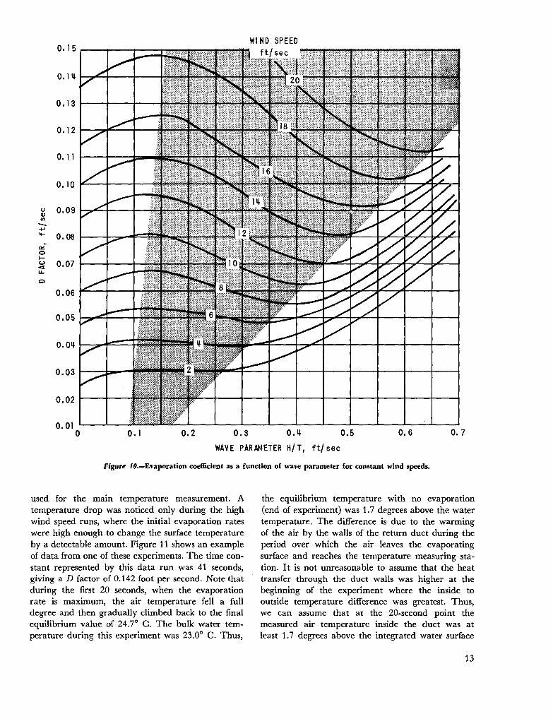
The presentation of experimental results in figure9 is appropriate for use in evaporation rate computa­tions. The variation of evaporation coefficient Dwith wave characteristics is more obvious in a pre­sentation of the same data showing D as a functionof wave parameter Hj T for constant values of windspeed as given in figure 10. An unexpected featurementioned earlier is immediately evident in figure 10.A large region exists (shaded area in the figure) inwhich the evaporation coefficient actually decreaseswith increasing wave action and the inverse relation­ship becomes more pronounced at higher wind speeds.This type of behavior was not anticipated at thebeginning of the study but appears to be a significantfeature of the wave tank results. It is clear that anunderstanding of the mechanisms that control Dmust include an explanation of this phenomenon.The experiments described below were conductedin attempts to explain this behavior.

1. Surface temperature studyUpon completion of the evaporation measurements

and having noted some of the peculiarities in theresults, an attempt was made to determine the causesof the observed behavior. One evaporation retardingmechanism that must be considered is the possiblereduction in surface temperature due to the evapora­tion itself. An infra-red thermometer was installed inthe tank with the sensor viewing the water surface.The intent was to measure the water surface tem­perature under many different surface and evapora­tion conditions. However, no significant differencesin temperature could be detected. Failure of the IRthermometer to detect surface temperature changeswas not considered conclusive since it was thoughtthat the instrument was being influenced by radia­tion from the walls and ceiling of the duct whichwas reflected into the sensor from the water surface.

While the simple IR thermometer installationfailed to detect surface temperature changes, thesechanges were in fact detected by the duct thermistor

(18)

(19)0.622e

q""'"--p

12

0.15

0.14

0.13

0.12

0.11

0.10

0 0.09Q)(/)-......... 0.08

0::0t-(.) 0.07«u..

c

0.06

0.05

0.04

0.03

0.02

0.010 0.1 0.2 0.3 0.4 0.5

WAVE PARAMETER HIT, ttl sec

0.6 O. 7

Figure lO.-Evaporation coefficient as a function of wave parameter for constant wind speeds.

used for the main temperature measurement. Atemperature drop was noticed only during the highwind speed runs, where the initial evaporation rateswere high enough to change the surface temperatureby a detectable amount. Figure 11 shows an exampleof data from one of these experiments. The time con­stant represented by this data run was 41 seconds,giving a D factor of 0.142 foot per second. Note thatduring the first 20 seconds, when the evaporationrate is maximum, the air temperature fell a fulldegree and then gradually climbed back to the finalequilibrium value of 24.7° C. The bulk water tem­perature during this experiment was 23.0° C. Thus,

the equilibrium temperature with no evaporation(end of experiment) was 1.7 degrees above the watertemperature. The difference is due to the warmingof the air by the walls of the return duct during theperiod over which the air leaves the evaporatingsurface and reaches the temperature measuring sta­tion. It is not unreasonable to assume that the heattransfer through the duct walls was higher at thebeginning of the experiment where the inside tooutside temperature difference was greatest. Thus,we can assume that at the 20-second point themeasured air temperature inside the duct was atleast 1.7 degrees above the integrated water surface

13

lpECIF!C HUML,TY

~,.-

~

v ,......

/\ /\ J

V

V TEMPERATURE[L--.Ir--*- ..... --1----_ 1--- ...~

-,"'-

t\ ..... -1~ .....

I.-'

\ ~ ..... ~

.//r"'- -

26

u0

lJJeo::::::>I-~eo::lJJQ..:z: 25lJJI-

eo::~

2~

o 2 3

TIME I N MINUTES

20

18

I ~

J~

01-'C-12 E01

>-10 l-

e%::::>

8 :z:uLL.

6 ulJJQ..

""~

2

o5

Figure ll.-Temperature and humidity as a function of time, Experiment No. 108.

temperature. This assumption is certainly on theconservative side, but it still places the water surfacetemperature at 22.5° C, or 0.5 degree below thebulk water temperature. Although the temperaturedrop is small and not likely to be significant in re­ducing evaporation rates, its presence is rather sur­prising in view of the violent water surface agitationby wind and waves taking place during the experi­ment.

2. Air flow tracingAnother possible reason for the decrease in evapo­

ration rate with increasing wave steepness is thereduction of vertical mass transport due to modifica­tion of the air flow and turbulence characteristics. Inorder to investigate this postulate, apparatus was setup in the wave tank to inject tracers into the airstream above the water.

The first method used was to inject neutrallybuoyant soap bubbles inflated with helium into theair flow above the water (Schooley). Movies weretaken with a 16 mm camera running at approxi­mately 50 frames per second. Displaying thesepictures at 8 frames per second uncovered some inter­esting flow structure around well-developed waves.

14

Figure 12 is an example of several consecutive framesshowing a bubble in a typical stationary position(relative to the wave) just in the lee of a wave crest.The same sequence shows other bubbles at higheraltitudes moving with the wind speed, which was 2to 3 times the wave phase velocity. Similar data wereanalyzed frame by frame, plotting bubble trajectories.Typical trajectories over small, wind-driven capillariesare shown in figure 13. Note the fairly uniform motionat all levels. Figure 14, in turn, shows bubble trajec­tories in the presence of well-developed waves. Notethat the upper flow is relatively undisturbed but thelow level circulation is completely changed. Circula­tion patterns coupled to the wave profile are im­mediately evident.

In another series of experiments, air motions weretraced by releasing chemical vapor plumes near thewaves and photographing- the plumes with thecamera. Air, saturated with titanium tetrachloride(TiCI4) , was pumped through the same bubblegenerators used in the bubble tests. TiCl4 reacts withwater vapor to form a fairly dense white cloud ofhydrogen chloride. The fumes are toxic, of course,but the experiments were carried out in the sealed

Figure 12.-Helium bubble stationary behind wave crest.

15

Figure H.-Bubble trajectories over surface with only wind-driven capillary waves present.

evaporation tank and no particular difficulties wereencountered. The tank environment was ideal forthis type of tracer since the experiments could be runat almost 100 percent relative humidity, the condi­tion necessary for maximum reaction of the TiCI4•

Figures 15, 16, 17, and 18 show typical frames fromthis series of pictures. In figure 15a, the vaporplume traces an upward flow as the wave crest ap­proaches. This flow continues to the front edge of thewave (figure 15c), then shifts to downward flow on

Figure H.-Bubble trajectories over weII-developed waves.

16

Figure H.-Smoke tracers over well-developed waves.

17

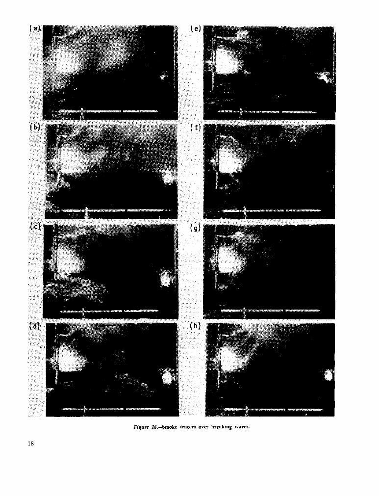
Figure 16.-Smoke tracers over breaking waves.

18

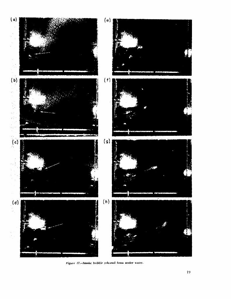
Figure J7.-Smoke bubble released from under water.

19

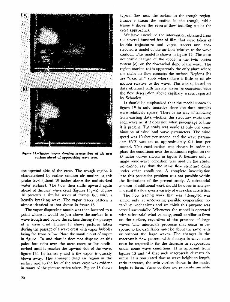
'ifure 1,.-Smoke tracers showing reverse How of air nearIUrfaee ahead of approaching wave crest.

the upwmd side of the crest. The trough region ischaracterized by rather random air motion at thisprobe level (about 10 inches above the undisturbedwater surface). The flow then shifts upward againahead of the next wave crest (figures 15g-h). Figure16 presents a similar series of frames but with aheavily breaking wave. The vapor tracer pattern isalmost identical to that shown in figure 15.

The vapor dispensing nozzle was then lowered to apoint where it would be just above the surface in awave trough and below the surface during the passageof a wave crest. Figure 17 shows pictures takenduring the passage of a wave crest with vapor bubblesbeing fed from below. Note the small cloud of vaporin figure 17a and that it does not disperse at thispoint but rides over the crest more or less undis­turbed until it reaches the upwind side of the wave,figure 17f. In frames g and h the vapor is quicklyblown away. This apparent dead air region at thesurface and to the lee of the wave crest was evidentin many of the picture series taken. Figure 18 shows

20

typical flow near the surface in the trough region.Frame a traces the motion in the trough, whileframe b shows the reverse flow building up as thecrest approaches.

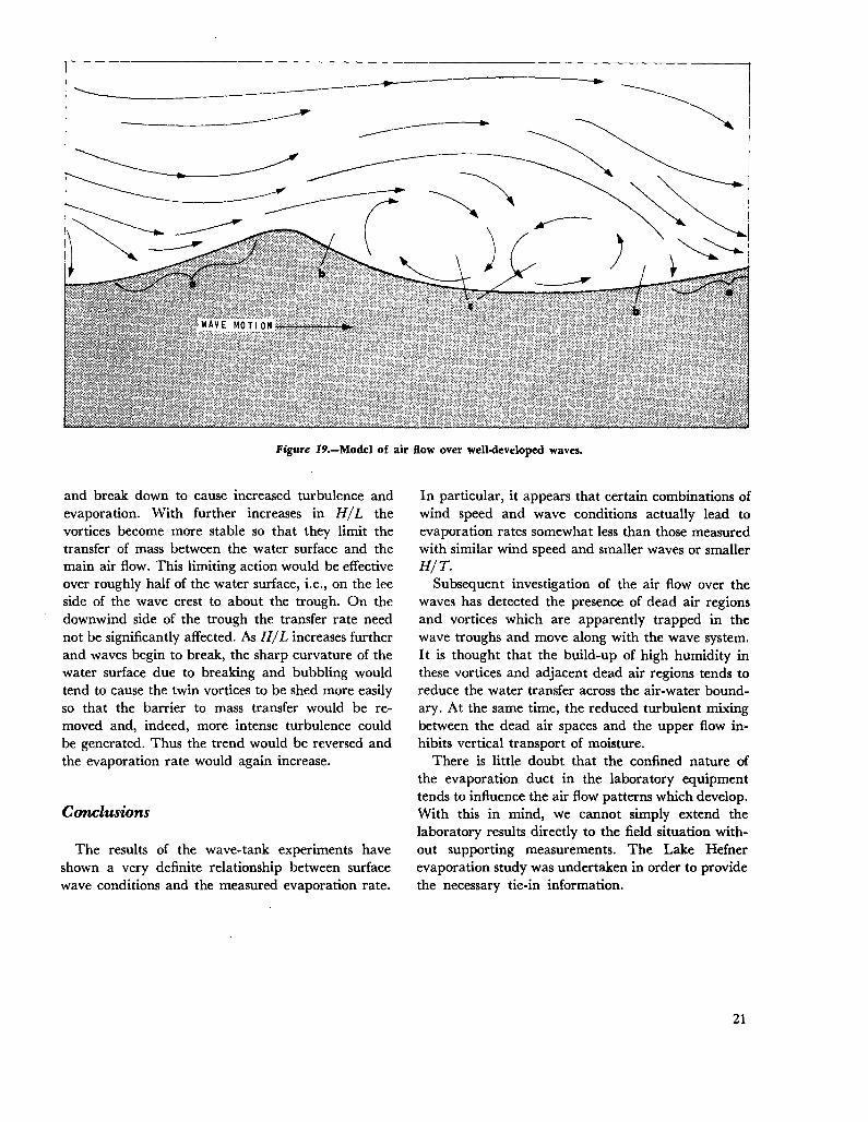
We have assembled the information obtained fromthe several hundred feet of film that were taken ofbubble trajectories and vapor tracers and con­structed a model of the air flow relative to the wavecontour. This model is shown in figure 19. The mostnoticeable feature of the model is the twin vortexsystem (c), on the downwind slope of the wave. Theregion marked (a) is apparently the only place wherethe main air flow contacts the surface. Regions (b)are "dead air" spots where there is little or no airmotion relative to the wave. This model, based ondata obtained with gravity waves, is consistent withthe flow description above capillary waves reportedby Schooley.

It should be emphasized that the model shown infigure 19 is only tentative since the data sampleswere relatively sparse. There is no way of knowingfrom existing data whether this structure exists overeach wave or, if it does not, what percentage of timeit is present. The study was made at only one com­bination of wind and wave parameters. The windspeed was 10 feet per second and the wave param­eter HI T was set at approximately 0.4 foot persecond. This combination was chosen in order toplace the conditions near the minimum region on theD factor curves shown in figure 9. Because only asingle wind-wave condition was used in the study,we cannot say that the same flow structure existsunder other conditions. A complete investigationinto this particular problem was not possible withinthe limitations of the present study. A substantialamount of additional work should be done to analyzein detail the flow over a variety of wave characteristics.

The flow tracing work that was attempted wasaimed only at uncovering possible evaporation re­tarding mechanisms and we think this purpose wasserved successfully. Whenever the tunnel is operatedwith substantial wind velocity, small capillaries formon the surface, regardless of the presence of largewaves. The microscale processes that occur in re­sponse to the capillaries must be about the same withor without the large waves. The changes in themacroscale flow pattern with changes in wave statemust be responsible for the decrease in evaporationunder some wave conditions. It is apparent fromfigures 13 and 14 that such macroscale changes dooccur. It is postulated that as wave height to lengthratio increases, the twin vortices shown in the modelbegin to form. These vortices are probably unstable

----~..-------------

Figure 19.-Model of air flow over well-developed waves.

and break down to cause increased turbulence andevaporation. With further increases in HIL thevortices become more stable so that they limit thetransfer of mass between the water surface and themain air flow. This limiting action would be effectiveover roughly half of the water surface, i.e., on the leeside of the wave crest to about the trough. On thedownwind side of the trough the transfer rate neednot be significantly affected. As HIL increases furtherand waves begin to break, the sharp curvature of thewater surface due to breaking and bubbling wouldtend to cause the twin vortices to be shed more easilyso that the barrier to mass transfer would be re­moved and, indeed, more intense turbulence couldbe generated. Thus the trend would be reversed andthe evaporation rate would again increase.

Conclusions

The results of the wave-tank experiments haveshown a very definite relationship between surfacewave conditions and the measured evaporation rate.

In particular, it appears that certain combinations ofwind speed and wave conditions actually lead toevaporation rates somewhat less than those measuredwith similar wind speed and smaller waves or smallerHIT.

Subsequent investigation of the air flow over thewaves has detected the presence of dead air regionsand vortices which are apparently trapped in thewave troughs and move along with the wave system.I t is thought that the build-up of high humidity inthese vortices and adjacent dead air regions tends toreduce the water transfer across the air-water bound­ary. At the same time, the reduced turbulent mixingbetween the dead air spaces and the upper flow in­hibits vertical transport of moisture.

There is little doubt that the confined nature ofthe evaporation duct in the laboratory equipmenttends to influence the air flow patterns which develop.With this in mind, we cannot simply extend thelaboratory results directly to the field situation with­out supporting measurements. The Lake Hefnerevaporation study was undertaken in order to providethe necessary tie-in information.

21

THE LAKE HEFNER EVAPORATION STUDY

(21)

Instrumentation at Lake Hefner

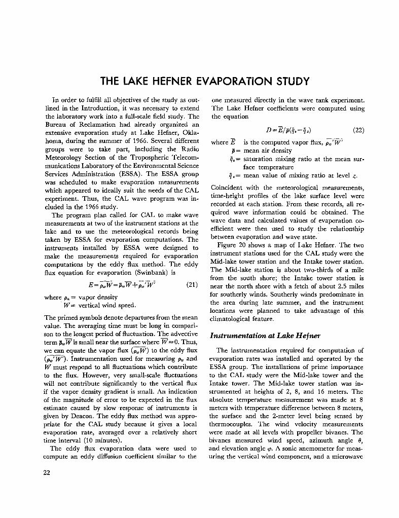
one measured directly in the wave tank experiment.The Lake Hefner coefficients were computed usingthe equation

The instrumentation required for computation ofevaporation rates was installed and operated by theESSA group. The installations of prime importanceto the CAL study were the Mid-lake tower and theIntake tower. The Mid-lake tower station was in­strumented at heights of 2, 8, and 16 meters. Theabsolute temperature measurement was made at 8meters with temperature difference between 8 meters,the surface and the 2-meter level being sensed bythermocouples. The wind velocity measurementswere made at all levels with propeller bivanes. Thebivanes measured wind speed, azimuth angle 8,and elevation angle 'P. A sonic anemometer for meas­uring the vertical wind component, and a microwave

(22)D=Ejp(q.-qz)

where E is the computed vapor flux, p,v' W'p= mean air density

q. = saturation mixing ratio at the mean sur­face temperature

qz = mean value of mixing ratio at level z.

Coincident with the meteorological measurements,time-height profiles of the lake surface level wererecorded at each station. From these records, all re­quired wave information could be obtained. Thewave data and calculated values of evaporation co­efficient were then used to study the relationshipbetween evaporation and wave state..

Figure 20 shows a map of Lake Hefner. The twoinstrument stations used for the CAL study were theMid-lake tower station and the Intake tower station.The Mid-lake station is about two-thirds of a milefrom the south shore; the Intake tower station isnear the north shore with a fetch of about 2.5 milesfor southerly winds. Southerly winds predominate inthe area during late summer, and the instrumentlocations were planned to take advantage of thisclimatological feature.

In order to fulfill all objectives of the study as out­lined in the Introduction, it was necessary to extendthe laboratory work into a full-scale field study. TheBureau of Reclamation had already organized anextensive evaporation study at Lake Hefner, Okla­homa, during the summer of 1966. Several differentgroups were to take part, including the RadioMeteorology Section of the Tropospheric Telecom­munications Laboratory of the Environmental ScienceServices Administration (ESSA). The ESSA groupwas scheduled to make evaporation measurementswhich appeared to ideally suit the needs of the CALexperiment. Thus, the CAL wave program was in­cluded in the 1966 study.

The program plan called for CAL to make wavemeasurements at two of the instrument stations at thelake and to use the meteorological records beingtaken by ESSA for evaporation computations. Theinstruments installed by ESSA were designed tomake the measurements required for evaporationcomputations by the eddy flux method. The eddyflux equation for evaporation (Swinbank) is

E=pwW=pwW+pw'W'

where PrJ; = vapor densityW = vertical wind speed.

The primed symbols denote departures from the meanvalue. The averaging time must be long in compari­son to the longest period of fluctuation. The advectiveterm PwW is small near the surface where W:::: O. Thus,we can equate the vapor flux (Pw W) to the eddy flux(Pw'W'). Instrumentation used for measuring pw andW must respond to all fluctuations which contributeto the flux. However, very small-scale fluctuationswill not contribute significantly to the vertical fluxif the vapor density gradient is small. An indicationof the magnitude of error to be expected in the fluxestimate caused by slow response of instruments isgiven by Deacon. The eddy flux method was appro­priate for the CAL study because it gives a localevaporation rate, averaged over a relatively shorttime interval (10 minutes).

The eddy flux evaporation data were used tocompute an eddy diffusion coefficient similar to the

22

1000 0H H H

A15

RAFT - 2[!)

13

6 THERMAL SURVEY STATION

~ FILM DISTRIBUTION LINES

SCALE IN FEET

1000 2000 3000I I

A33

4000!

---

A18

- - - - IZQ9__INTAKE TOlER

A INSTRUIIENT STATION17

RAFT-~

22

A23

A24

A3

834

827

RAFT- 4

6, r9\

MID-LAKE TOWERINSTRUMENT STATION

Figure ZO.-Map of Lake Hefner, Oklahoma City, Okla.

refractometer for sensing fluctuations in humidity,were located at the 8-meter level. Barium florideresistance strips were used at all levels for measuringthe relative humidity.

Similar instruments were installed at the Intaketower with the exception of the sonic anemometer andrefractometer. Only the 2-meter and the 8-meter

levels were instrumented at the Intake tower. Meas­urement stations were also located at the east sideand the south side of the lake, but the data from thesesites were not used in the CAL study.

Measurement of wave conditions was undertakenby CAL as part of the extended wave-evaporationstudy. The instrument designed for the wave meas-

23

ELECTRODE 1

TEFLON

01 ELECTRIC

ELECTRODE 2 v

CRw

WATER

r 3"-1(a) PROBE

Figure 21.-Basic wave probe configuration.

(b) EQUIVALENT CIRCUIT

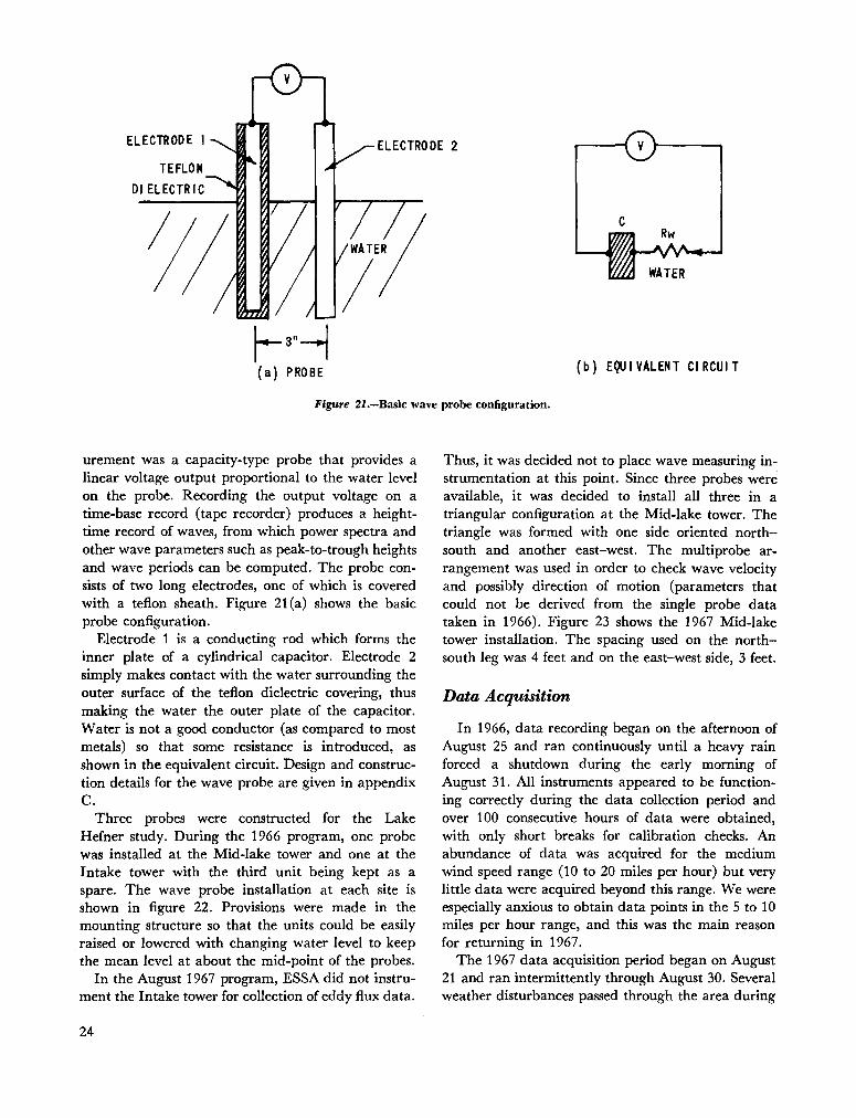
urement was a capacity-type probe that provides alinear voltage output proportional to the water levelon the probe. Recording the output voltage on atime-base record (tape recorder) produces a height­time record of waves, from which power spectra andother wave parameters such as peak-to-trough heightsand wave periods can be computed. The probe con­sists of two long electrodes, one of which is coveredwith a teflon sheath. Figure 21 (a) shows the basicprobe configuration.

Electrode 1 is a conducting rod which forms theinner plate of a cylindrical capacitor. Electrode 2simply makes contact with the water surrounding theouter surface of the teflon dielectric covering, thusmaking the water the outer plate of the capacitor.Water is not a good conductor (as compared to mostmetals) so that some resistance is introduced, asshown in the equivalent circuit. Design and construc­tion details for the wave probe are given in appendixC.

Three probes were constructed for the LakeHefner study. During the 1966 program, one probewas installed at the Mid-lake tower and one at theIntake tower with the third unit being kept as aspare. The wave probe installation at each site isshown in figure 22. Provisions were made in themounting structure so that the units could be easily

.raised or lowered with changing water level to keepthe mean level at about the mid-point of the probes.

In the August 1967 program, ESSA did not instru­ment the Intake tower for collection of eddy flux data.

24

Thus, it was decided not to place wave measuring in­strumentation at this point. Since three probes wereavailable, it was decided to install all three in atriangular configuration at the Mid-lake tower. Thetriangle was formed with one side oriented north­south and another east-west. The multiprobe ar­rangement was used in order to check wave velocityand possibly direction of motion (parameters thatcould not be derived from the single probe datataken in 1966). Figure 23 shows the 1967 Mid-laketower installation. The spacing used on the north­south leg was 4 feet and on the east-west side, 3 feet.

Data Acquisition

In 1966, data recording began on the afternoon ofAugust 25 and ran continuously until a heavy rainforced a shutdown during the early morning ofAugust 31. All instruments appeared to be function­ing correctly during the data collection period andover 100 consecutive hours of data were obtained,with only short breaks for calibration checks. Anabundance of data was acquired for the mediumwind speed range (10 to 20 miles per hour) but verylittle data were acquired beyond this range. We wereespecially amcious to obtain data points in the 5 to 10miles per hour range, and this was the main reasonfor returning in 1967.

The 1967 data acquisition period began on August21 and ran intermittently through August 30. Severalweather disturbances passed through the area during

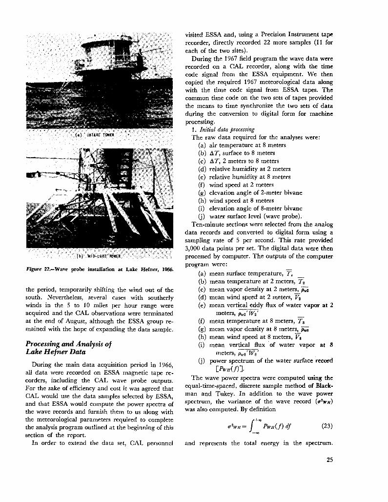
Figure 22.-Wave probe installation at Lake Hefner, 1966.

the period, temporarily shifting the wind out of thesouth. Nevertheless, several cases with southerlywinds in the 5 to 10 miles per hour range wereacquired and the CAL observations were terminatedat the end of August, although the ESSA group re­mained with the hope of expanding the data sample.

Processing and Analysis ofLake Hefner Data

During the main data acquisition period in 1966,all data were recorded on ESSA magnetic tape re­corders, including the CAL wave probe outputs.For the sake of efficiency and cost it was agreed thatCAL would use the data samples selected by ESSA,and that ESSA would compute the power spectra ofthe wave records and furnish them to us along withthe meteorological parameters required to completethe analysis program outlined at the beginning of thissection of the report.

In order to extend the data set, CAL personnel

visited ESSA and, using a Precision Instrument taperecorder, directly recorded 22 more samples (11 foreach of the two sites).

During the 1967 field program the wave data wererecorded on a CAL recorder, along with the timecode signal from the ESSA equipment. We thencopied the required 1967 meteorological data alongwith the time code signal from ESSA tapes. Thecommon time code on the two sets of tapes providedthe means to time synChronize the two sets of dataduring the conversion to digital form for machineprocessing.

1. Initial data processingThe raw data required for the analyses were:

(a) air temperature at 8 meters(b) .1T, surface to 8 meters(c) .1T, 2 meters to 8 meters(d) relative humidity at 2 meters(e) relative humidity at 8 meters(f) wind speed at 2 meters(g) elevation angle of 2-meter bivane(h) wind speed at 8 meters(i) elevation angle of 8-meter bivane(j) water surface level (wave probe).

Ten-minute sections were selected from the analogdata records and converted to digital form using asampling rate of 5 per second. This rate provided3,000 data points per set. The digital data were thenprocessed by computer. The outputs of the computerprogram were:

(a) mean surface temperature, T.(b) mean temperature at 2 meters, T2

(c) mean vapor density at 2 meters, PUJ2

(d) mean wind speed at 2 meters, V2

(e) mean vertical eddy flux of water vapor at 2meters, Pw2' W2 '

(f) mean temperature at 8 meters, Ts(g) mean vapor density at 8 meters, PVJS

(h) mean wind speed at 8 meters, Vs(i) mean vertical flux .of water vapor at 8

meters, Pws' Ws'

(j) power spectrum of the water surface record[PWH(J)].

The wave power spectra were computed using theequal-time-spaced, discrete sample method of Black­man and Tukey. In addition to the wave powerspectrum, the variance of the wave record (0'2WH)was also computed. By definition

(23)

and represents the total energy in the spectrum.

25

Figure 2J.-Wave probe installation at the Mid-lake tower, 1967.

frequency

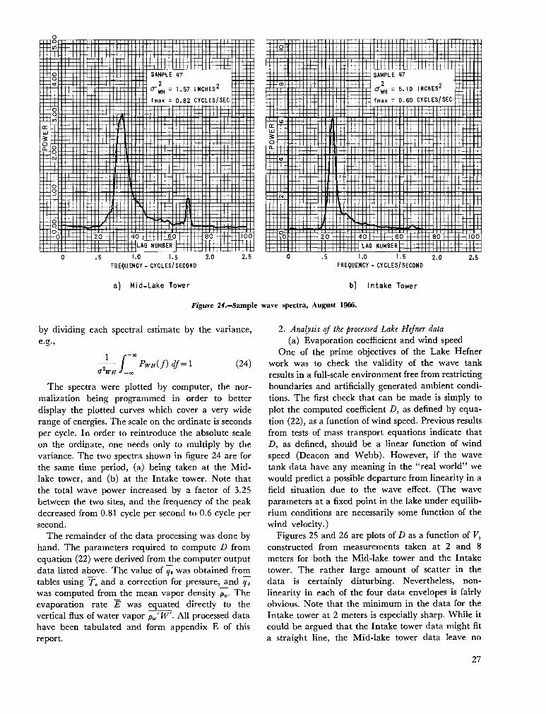
Figure 24 shows sample spectra computed from theLake Hefner data. The numbers plotted along theabscissa are lag numbers from the computationprocess and represent frequency. The frequency corre­sponding to the lag number can be computed from

26

the simple relationship,

lag number100 X 2.5 cycles per second

The spectra have all been normalized to unit area

20 40 60 80 1000

0 20 40 60 80 100LAG NUMBER LAG NUMBER

.5 1.0 1.5 2.0 2.5 0 .5 1.0 1.5 2.0 2.5FREQU ENCY - CYCLES/ SECOND FREQUENCY - CYCLES/ SECOND

00Iti

00<i

00".;

0::l.LJ3:°0a.. 0

N

0~

00ci

0

0

SAMPLE 1172

o-WH 1.57 INCHES 2

fmax D.B2 CYCLES/SEC

a) Mid-Lake Tower

0::l.LJ3:

°a..

o

CD

N

SAMPLE 117

o-;H 5. 10 I NCHES2

fmax 0.60 CYCLES/SEC++~~

b) Intake Tower

Figure U.-Sample wave spectra, August 1966.

by dividing each spectral estimate by the variance,e.g.,

The spectra were plotted by computer, the nor­malization being programmed in order to betterdisplay the plotted curves which cover a very widerange of energies. The scale on the ordinate is secondsper cycle. In order to reintroduce the absolute scaleon the ordinate, one needs only to multiply by thevariance. The two spectra shown in figure 24 are forthe same time period, (a) being taken at the Mid­lake tower, and (b) at the Intake tower. Note thatthe total wave power increased by a factor of 3.25between the two sites, and the frequency of the peakdecreased from 0.81 cycle per second to 0.6 cycle persecond.

The remainder of the data processing was done byhand. The parameters required to compute D fromequation (22) were derived from the computer outputdata listed above. The value of q. was obtained fromtables using T. and a correction for pressure, and qz

was computed from the mean vapor density Pw' Theevaporation rate E was equated directly to thevertical flux of water vapor Pw' W'. All processed datahave been tabulated and form appendix E of thisreport.

1 f+CO-2- PwH(J) dj= 1U WH -co

(24)

2. Analysis of the processed Lake Hefner data(a) Evaporation coefficient and wind speed

One of the prime objectives of the Lake Hefnerwork was to check the validity of the wave tankresults in a full-scale environment free from restrictingboundaries and artificially generated ambient condi­tions. The first check that can be made is simply toplot the computed coefficient D, as defined by equa­tion (22), as a function of wind speed. Previous resultsfrom tests of mass transport equations indicate thatD, as defined, should be a linear function of windspeed (Deacon and Webb). However, if the wavetank data have any meaning in the "real world" wewould predict a possible departure from linearity in afield situation due to the wave effect. (The waveparameters at a fixed point in the lake under equilib­rium conditions are necessarily some function of thewind velocity.)

Figures 25 and 26 are plots of Das a function of V,constructed from measurements taken at 2 and 8meters for both the Mid-lake tower and the Intaketower. The rather large amount of scatter in thedata is certainly disturbing. Nevertheless, non­linearity in each of the four data envelopes is fairlyobvious. Note that the minimum in the data for theIntake tower at 2 meters is especially sharp. While itcould be argued that the Intake tower data might fita straight line, the Mid-lake tower data leave no

27

I I I I I I I T T

MID-LAKE TOWER - 2 METERS

~0 - FREE WATER SURFACE

0 b. - SUSPECTED PRESENCE OF F

100_ 1

\ /\

0 1\ I

\" /,/0 0

0 ,~ 0-"

0-- A!~I

~. 0 00

,00 0 I,0 0 0 " 0

I

"- 0 0 0 I

"-~ 00 /

'"0

*' o 0 P '"0- .... 0 ...." -A I" " "

! 1 0

1

I I 0,i

I I 0, 01

\ 1 0

~ 1 0

~ 1\ ,/\ _I 0

0

" 1/ 0 00~"

"- ",/ 0 17....-' 0 '" ,/- 0 '~

0 / 0C 0 o~/

u0 0 "" 0 0 0 '"

0u u 0 ....

1'-- .... o 0 0 g..- ;' MID-LAKE TOWER - 8 METERS.... --~-"_0--

00 - FREE WATER SURFACE

.. A - SUSPECTED PRESE~CE ~

.028

.021JuQ)

'"-+' .020~

I

Cl

~ .016zUJ

(,,)

...........012UJ

0(,,)

z0

~ .008cIll:0~

c>UJ .OOIJ

oo

.021JuQ)

'"-+'~ .020

Cl

~z .016UJ-(,,)..........UJ

.0120(,,)

z0

~

.008cIll:0~

c>UJ

.OOIJ

oo

2 3 IJ 5 6 7 82 METER WIND SPEED - METERS PER SECOND

a) Computed From The 2 Meter Level Data

2 3 ~ 5 6 7 8

8 METER WIND SPEED - METERS PER SECOND

b) Computed From The 8 Meter Level Data

9

9

ILM

10

F FILM

10

28

Figure 2J.-Evaporation coeflicient D as a function of wind speed, Mid·lake tower.

1092 3 ij 5 6782 METER WIND SPEED - METERS PER SECOND

a) Computed From The 2 Meter Level Data

I I I I I I I 1 II--~INTAKE TOWER - 2 METERS

o - FREE WATER SURFACEI'0

~ f-

~ - SUSPECTED PRESENCE OF FILM,I

ttl

0Ir, 1 I\ j

I i\ 0 1/ 0 6

\ /I

c 00 / o I

'\ 0 ' .. 0 /o c ....- ... 00 /I"'~

~o... ft ~,..- •666

"6

.Oij8

.032

.0ijO

.008

.056

oo

o....z:UJ

uu..u..UJ

8 .02ijz:o....~ .016oQ..e:[:>­UJ

uG)II)­........

102 3 ~ 5 6 7 8

8 METER WIND SPEED - METERS PER SECOND

b) Computed From The 8 Meter Level Data

INTAKE TOWER - 8 METERSI

/-f- Io - FREE WATER SURFACE /

- .... I

~ - SUSPECTED PRESENCE OF FILM II

I 0

ft L'\

/ 0~, c

~,/ 0 /......0 I

0 0 0 IQ d 0

I0 00

c 00 • /0 /

" 1,. .........P... -..

~/t'1..-'"---1---- 6

6

"6

66

"6

oo

.056

u .Oij8G)II)-........

.0ijO0

....z:UJ

u •032u..u..UJ0u .02ijz:0-....e:[e:t:

.0160a..e:[:>-UJ

.008

Figure 26.-Evaporation coefficient D as a function of wind speed, Intake tower.

29

~~~,.:• I I I I I I I \~~~~V 0- ~ VARIANCE OF WAVE HEIGHT

AS A FUNCTION OF 2 METER 0~/- ~ WIND SPEED

~("'>

V/ ~~~-

'\~/ ')C. <c..-"'--

7~~

'/ I.t. / .'~'/ ~ -\'"

./

f y V

r/ ..L/'

pt0 ./'i

YV7"7'

7

6

5N

II)

CD.J::U Ij.C

I

:c~ 3wCo)z~

ao:~ 2>-

oo 2 3 Ij. 5 6 72 METER WIND SPEED - METERS PER SECOND

Figure 27.-Total wave energy as a function of the 2·meter wind speed.

8 9

doubt about the existence of a minimum in D for windspeeds of 4 to 5 meters per second.

(b) Wave data analysisIn order to make a comparison between laboratory

results and Lake Hefner data, the Lake Hefner wind­wave relationships are required. Twenty-four wavepower spectra were computed, representing the fullrange of wind speeds encountered during the fieldstudies. The spectra were all strongly peaked withlittle wave energy outside the significant wave fre­quency. The peak frequency could be read veryeasily from each spectrum. This frequency was deter­mined and converted to wave period.

Along with wave spectra, the variance or totalwave energy was also computed. By taking thesquare root of the variance we obtain the standarddeviation of the wave record. Since the spectra indi­cate very strongly monochromatic waves, and sincethe waves are nearly sinusoidal in shape, it is not un­realistic to equate the measured standard deviationto the rms value of an equivalent sine wave. The peak­to-trough wave height may then be estimated usingthe expression:

(25)

30

The wave spectra and the variance thus provided thenecessary information for computing the wave param­eter HIT. Figure 27 presents a plot of wave energy(U 2WH) as a function of 2-meter wind speed for boththe Mid-lake tower and the Intake tower. Note thatat a wind speed of 7 to 8 meters per second the waveenergy at the Mid-lake tower is still increasing at anear constant rate, while the wave energy at theIntake tower is beginning to reach a maximum.Figure 28 shows the wave parameters or wave height­to-period ratio (HI T) for both sites. Again the Mid­lake tower curve is linear, while that for the Intaketower has a parabolic shape due to the amplitudelimiting occurring over the much longer fetch.

Since the wave parameter versus wind speed curveis linear for the Mid-lake tower, a plot of the coeffi­cient D versus HI T would show a distribution similarto those in figures 25 and 26. However, this is notnecessarily true for the Intake tower. Figure 29 showsa plot of D as a function of HI T for the 2-meter levelat the Intake tower. Although the (HIT, V) rela­tionship is nonlinear, this has not appreciably alteredthe D coefficient envelope. The gross departure fromlinearity and the minimum (at HIT=0.3) remainsas in the wind-dependent curves.

·~

(,)Q)

~ .3........

I­­•

.2

I I I Ix - MID-LAKE TOWERo - INTAKE TOWER ~<c,~

,,<c,~~

~,{ .L0 --1--~llfr4K."," V" ~ E: rolf,

II.;. a[;/ b>V

/-/

/17

~I X

PI' L?~;,V

I~110

X ,V Vav'X

oo 2 3 ~ 5 6

2 METER WIND SPEED - METERS PER SECOND7 8 9

Figure 28.-Wave parameter HIT as a function of the 2·meter wind speed.

I0

II

0I

I I0 I ,

I ,!

0/ I If0- "' ....

I I....- !, .... ' .... I" I~

........ " I8

Ib,....... 0 )-. I I

0 " o~ l/oI

p b 'l:l..... I I

1-- / L/_..... -- -- "0 y ..... .........

I"- _.[;/,,-' 0

,.",.

. 056

.0~8(,)Q)II)-........

.O~O

0

I-z: .032UJ

<,)

I.LI.LUJ

.02~0<,)

z:0

I- .016oCI:0:::0"-oCI:>UJ

.008

00.20 0.25 0.30

WAVE PARAMETER HIT - ft/sec

0.35

Figure 2,.-Evaporation coefficient D as a function of the wave parameter HIT for the 2-meter level at the Intake tower.

31

COMPARISON OF THE LABORATORY

AND FIELD RESULTS

In the laboratory experiments, there was littlecorrelation between wind and waves since they weregenerated independently. Because there was no wayof knowing just what range of wave characteristicswould correspond to given wind velocities in the field,the tank experiments were run over the completerange of wind speed and wave parameters attainablewith the apparatus. Many of these data lie outsidethe range likely to occur in the field. We can, however,~ompare the two sets of data through the wavemeasurements made at Lake Hefner.

The H/ T versus V curves for Lake Hefner (figure28) were plotted on the D(H/T, V) field computedfrom the wave tank measurements (figure 9). Thiscombination makes possible the construction of a Dversus wind speed curve using the tank evaporationdata. As was anticipated, this curve showed a sub­stantially different relationship from that found onLake Hefner (figures 25 and 26). However, it is pos-

sible to reconcile the two sets of data by a relativelysimple adjustment of the wave tank results. Figures30(a) and 30(b) show the D(H/T, V) field requiredto duplicate the Lake Hefner results. Note that thegeneral shape of the D contours remains the same asin the wave tank; it has been necessary only torotate the field clockwise about the origin and scalethe coefficient values by a fixed amount. The reasonfor the scaling factor is quite understandable and wasdiscussed previously under "Results of the WaveTank Evaporation Experiments." On the other hand,the necessity to rotate the wave-tank-derived D con­tours is most surprising. As is readily seen in figures30(a) and 30(b), the rotation process has increasedthe negative slope to the left of the peak. Thus, weare led to conclude that in the field situation, the in­fluence on evaporation by waves on the surface ap­pears to be even greater than in the wave tank.

33

o.OO~ -- -' Y"./ I

.L, .... -.... /.006 ~ i--"I __ -~

.008- -1---+-.0107~-- --

~

, I jlt' I II !/I !

I Y I II ~V! I

o~ S

I--+--+--+--+--~-~-+--+--+--+-:::I"-U)-O - .--t---f~ (; ~ i/~

-- 0 - • -4H"L-I--+----+o ~ ,. I! j.~~ I lY! I

.350Ql1/1-+'~

.... .30-:z:::D::LIJ....LIJ:IE:ooccD::oocc .25A.

LIJ>oocc3:

.20

983 ~ 5 6 7

2 METER WIND SPEED - METERS PER SECOND

a) Mid-Lake Tower - 2 Meter Data

0L--l..._...L..--..l._...l..._L--.1.._..L----J._~_L....___L.._.L._........L_____'

2

.35

0Ql1/1- .30+'~

....-:z:::D::LIJ.... .25LIJ:IE:ooccD::ooccA.

LIJ>oocc3: .20

I:::I"~D°NONO·-~- .,-U-+f~ ~III I I

; fHIl-f IfY

"0 --;1/'/ I I

--- / IOl~

/

V: /-- v/- ".01617 ...... " ..-.020-7~- ...---

r1- ....1--

.02~-

o2 3 ~ 5 6 7

2 METER WIND SPEED - METERS PER SECOND

b) Intake Tower - 2 Meter Data

8 9

Figure JO.-Contours of <:onstant D as a fun<:tion of wave parameter HIT andwind speed-<:ontours adjusted to fit the Lake Hefner results.

34

EVAPORATION ESTIMATES AND WAVES

and

(28)

(29)

where E= evaporation in centimeters per 3 hoursVs= wind speed in knots at 8 meters 'l1e = vapor pressure difference in millibars.

where E= evaporation in inches per dayV4 = wind speed in miles per day at 4 metersl1e = vapor pressure difference in inches of

mercury.

Linsley, Kohler, and Paulhus also derived two equa­tions from slightly different data inputs,

and

E= 5.38 X 1O-5Vs(q,-qs)

E= 5.56 X10-5V,lq.-q..)

E= 6.65 X 10-5V4(q,-q2)

E= 5.92 X 1O-5V4(q,-Q2)

E= 6.17 X 10-5V2(q,-q2)

During 1965, Oklahoma State University, workingfor the Bureau of Reclamation, did yet anothersurvey of Lake Hefner. Fry reports two more estimatesof the mass transport coefficients, using both waterbudget and energy budget methods. The waterbudget form is:

where E= evaporation in centimeters per dayV2 = wind speed in kilometers per day at 2

metersl1e = vapor pressure difference in millibars.

All the above equations report a different value ofN because they each use different units. Since noneof the above forms match the units used in the CALstudy, we have chosen to transform these equationsto fit our units. The equations reduce to the following(in the order presented):

(27)

(26)

Although every attempt was made to make theLake Hefner study as quantitative as possible, therewas considerable scatter in the processed data andthe overall evaporation estimates were somewhatlower than existing water budget information wouldhave predicted. The reasons for the apparent inac­curacies in the evaporation estimates are very likelydue to departure from the ideal conditions assumedin developing the eddy flux theory. For example,neglecting the advective term Pw W by assumingW = 0, does not necessarily hold. In fact, the meanvertical wind was never zero in any of the processedsamples, although this could have been due to smallerrors in calibration of the bivanes. There was alsosome evidence that the humidity and wind measuringinstruments did not have fast enough response timesto follow all the significant eddy scales. Comparisonof the measured vapor fluxes from the Mid-lake towerand the Intake tower tend to suggest that the Mid­lake instruments were located on the outer fringe ofthe vapor blanket. Significantly lower values of thevapor density variance at the Mid-lake tower leadsus to this conclusion. The apparent thinness of thevapor blanket at the Mid-lake tower (if this is trulythe case) may be due to the reduction in verticaltransport of water vapor caused by the waves on thewater surface.

While the absolute measurements of evaporationmay be somewhat in error, changes in the measuredparameters relative to some chosen base value arethought to be more reliable. Thus, we have chosen touse the shape of the measured curve of mass transfercoefficient as a function of wind speed (and the de­pendent wave parameters), and to adjust the absolutemagnitude using the many available water-budget­derived values.

Marciano and Harbeck derived two empiricalequations of best fit for Lake Hefner, using slightlydifferent data for each. These are,

35

where the units are E: grams per centimeter squaredper second centimetersdecrease in water level persecond

V: feet per secondq: mixing ratio in grams per

gram.

(33)

(37)

(36)

then

but

the water budget studies. The mean value of N forthe water budget analyses described previously isN=5.93XI0- 5 centimeter/foot. In order to make theappropriate adjustments, it is required to know thewind speed distribution for the survey periods fromwhich the water budget values were derived. Thesedistributions were not available. However, we haveused the 2-meter wind speed distribution from thepresent Lake Hefner study as a realistic approxi­mation.

The method of adjustment is as follows:Let

+ jvmax

P(V2)n(V2) dV (35)o

where n(V2) = the average curve from the dataN(V2) = required N(V) curve

K = adjustment constant.

It is required to find K such that

N(V2)= jvmax

P(V2)N(V2) dV=5.93XI0- 5 (34)o

P(V2) = 2-meter wind speed probability density.

The averaging is done over the wind speed probabilitydensity curve derived from the Lake Hefner winddata.

Substituting equation (33) into equation (34)

5.93XlO-5=K jvmax

P(V2) dVo

The function P(V2)n(V2) was plotted as a function ofV2 and the integral evaluated using a planimeter.With the value of the integral computed, K was thendetermined from equation (37). The curve

(figure 32) is the adjusted curve and represents, asclosely as we are able to determine, the variation of ]v

with wind speed (and waves). The solid line offigure 32 is the final form of the N(V) relationshipdetermined by the CAL study. The dotted line offigure 32 is the water budget mean value of N.

(31)

(32)

Mid-lake tower E = 3.02 X 10-5V2(q. - q2)

Intake tower

Equation (31) was derived from the Mid-lake towerdata and equation (32) from the Intake tower meas­urements. Although the Intake tower coefficientagrees very well with the water budget values givenabove, the Mid-lake tower measurement appears tobe too low. Nevertheless, both measurements agreewell enough with the water budget data to justifyour acceptance of the quantitative estimate of thechanges in the mass transfer coefficient with windand waves.

The mass transport coefficients (N) were computedfor each of the available 10-minute samples from the1966-67 field programs. These data were plottedagainst wind speed and average curves determined byinspection, giving more weight to the points whichlay closer to the centroid of the group. These plotsare shown in figures 31a and 31b. The next stepwas to combine the average curves from the two sitesto obtain an average curve for the whole lake. Theresulting curve, while not being absolutely correct inmagnitude, is believed to represent the correctvariation of N with wind speed and associated wavestructure.

The average curve for N as determined by com­bining the data from the two Lake Hefner stationsmust now be adjusted to correspond to the meanvalue of the mass transport coefficient derived from

Note the close agreement of the equations in spiteof the slightly different measuring heights. Normallywe would expect the term Vt:.q to be somewhat largerfor 8 meters than for 2 meters, leading to lowervalues of N using 8-meter data. Although there isevidence of this effect in the above equations, thetotal spread in the values is small. In fact, the totalrange of values does not exceed the probable error inany individual estimate. Therefore, we have chosento combine the estimates as they stand and use themean value of N as the absolute reference for the CALdata.

The mean coefficients derived from the CAL studywhich correspond to the above are:

36

8

10

.

- ........... V

'" /

~-0

'" V 0 /-0- ..... 0 C /

00 "/;: V ~ ",-

....... ~1,./

~ .... 0 ..-0

"t> ......, " ..... 0 V10 0 1--0.- ~~ --(.......... -0- R. 0 -- -- ~

0 b r-- 0

1% ~ j.-'l7"'"0 1-0- -

+'....-5 6

LO

C)

)(

z:

2

oIJ 6 8 10 12 llJ 16 18 20

2 METER WIND SPEED - ft/sec

a) Mid-Lake Tower - 2 Meter Data,

22 21J

llJ

12

10

+'....-e 8u

o 6

)(

:z:

2

\0

\ / /~ / II

.'

......-- ..... 1\ !/ /"- /

1/ " 0 \ J 0/' 0 " /

/ 0"'; \ r7 7 /~, ~ ~d'\ '\~ / /0 17- o 0 / 16v

// ........... 'b ' .....~/ V"'- ~. 0

v~

0 - ./~,1 00 :-.... ./

r-- IV =-

oIJ 6 8 10 12 IIJ 16 18

2 METER WIND SPEED - ft/sec

b) Intake Tower - 2 Meter Data

20 22 21J

Figure JI .-Mass transfer coefficient N as a function of wind speed.

The N(V) curve presented in figure 32 is the"instantaneous" value of N for the equilibrium windspeed V. The term "instantaneous" refers to thelength of time the wind speed, and other parametersrequired in the evaporation estimate, remain rela-

tively constant. The curve was developed using meanmeasurements over lO-minute time intervals.

It should be emphasized that the variable N rela­tionship shown in figure 32 should not be used withlong-period averaged inputs. For example, if the wind

37

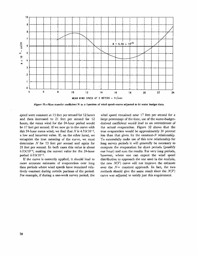
10

9

8

7........-- 6E

<.>

U'> 50

x ij

z:

3

2

./~

~v

.,-/ /~

VN = 5.93 x 10-5 /

~r--..... :/~- ...---V

oij 6 8 10 12 16 18 20 22

MEAN WIND SPEED AT 2 METERS - ft/sec

Figure J2.-Mass transfer coefficient N as a function of wind speed-curve adjusted to fit water budget data.

speed were constant at 13 feet per second for 12 hoursand then increased to 21 feet per second for 12hours, the mean wind for the 24-hour period wouldbe 17 feet per second. If we now go to the curve withthis 24-hour mean wind, we find that N is 4.3 X 10-5,

a low and incorrect value. If, on the other hand, werecognize the true meaning of the curve, we mustdetermine N for 13 feet per second and again for21 feet per second. In both cases this value is about6.0 X 10-5, making the correct value for the 24-hourperiod 6.0XlO-5•

If the curve is correctly applied, it should lead tomore accurate estimates of evaporation over longtime periods where wind speeds have remained rela­tively constant during certain portions of the period.For example, if during a one-week survey period, the

38

wind speed remained near 17 feet per second for alarge percentage of the time, use of the water-budget­derived coefficient would lead to an overestimate ofthe actual evaporation. Figure 32 shows that thetrue evaporation would be approximately 30 percentless than that given by the constant-N relationship.To successfully make use of this new relationship forlong survey periods it will generally be necessary tocompute the evaporation for short periods (possiblyone hour) and sum the results. For very long periods,however, where one can expect the wind speeddistribution to approach the one used in the analysis,the new N(V) curve will not improve the estimateover the N = constant approach. In fact, the twomethods should give the same result since the N(V)curve was adjusted to satisfy just this requirement.

CONCLUSIONS AND RECOMMENDATIONS

Despite certain difficulties with techniques andinstrumentation, some very useful results have beenobtained. The wave tank measurements showed thatwaves apparently modify the air flow over the surfacein such a way that turbulent transport mechanismscan be suppressed. Follow-up experiments conductedin the field tend to support the tank measurements,and in fact show that the evaporation retardingmechanism appears to be even more effective in thefield.

The results of both the laboratory and the fieldstudies tend to confirm the postulates of Stewart andthe theory of Phillips outlined in the Introduction.Organized flow does develop in the wave troughs, asdemonstrated by the flow tracing experiments in thewave tank. The consistent minima in the masstransport coefficient curves, developed from the LakeHefner data, tend to show a resonance effect for acertain combination of wind speed and HIT ratio.

No information was gained about the effect ofbreaking bubbles on evaporation rate. However, inview of the measurements made, it would seem thatthe controlling mechanism for evaporation from afree water surface is the turbulent transport mecha­nism, at least at light-to-moderate wind speeds. In awind regime where bubbling on the waves might beimportant, the wind-wave mechanism is in controland vertical transport of moisture is being retarded.At high wind speeds, spray and bubbles may well beimportant.

Although the work performed by CAL was notdesigned to evaluate evaporation-suppressing chemi­cals, use of these chemicals during certain periods ofthe Lake Hefner study was evident in the processeddata. Curiously enough, the mass transport coeffi­cients computed when the alcohol film was near oraround the measurement site, while being somewhatlower than the main bulk of data, displayed a similardependence on wind and waves. We might concludefrom this that the existence of the monolayer does notsignificantly alter the wave parameters that influencethe transport mechanisms. Unfortunately, we werenot able to obtain a significant sample of wave spectraduring periods of film application to make anyjudgment on the effect of monolayers on waves.

A mass transfer coefficient curve was developedwhich is applicable to short-period measurementsand takes into account the wind-wave interaction.This type of relationship will be valuable in futurework related to the evaluation of evaporation-re­tarding chemicals where it will be most desirable tohave a method of estimating short-term evaporationrates from the untreated surface.

Recommendations

While the results of the present study are encour­aging, much is yet to be learned about the air-waveinteraction. The results obtained at Lake Hefner arenot necessarily applicable to other lakes where differ­ent wind-wave characteristics may be present. This isespecially true of larger lakes where the fetch is muchlonger than on Lake Hefner.

It is therefore recommended that air-wave inter­action studies be continued with specific areas ofattention as follows:

1. Develop wind-wave and wind-evaporation ratestudies on a lake much larger than Hefner in orderto better assess the effect of fetch.

2. Attempt to determine the actual air flow whichdevelops over waves and formulate an analyticaldescription of this flow.

3. Determine the effect of monolayers on the wavere?;ime. There may be some interference effect suchas shifting the wave parameters out of the naturalresonance point.

4. Increase the accuracy of the eddy flux evapora­tion measurement technique and thus reduce thescatter in the computed data. With increased ac­curacy, the mass transfer characteristic could be com­puted directly without the necessity of adjustment tolong-period measurements which may have unknowninherent biases.

5. Extend the wind-wave and wind-evaporationstudies to much higher wind speeds in order todeduce: (a) the effect of spray on evaporation rates,and (b) the existence of higher "harmonics" of thenull effect found in the mass transport coefficient at17 feet per second wind speed.

39

REFERENCES

1. Blackman, R. B., and J. W. Tukey, 1959: The Measurementof Power Spectra from the Point of View of CommunicationsEngineers, New York, Dover Publications.

2. Deacon, E. L., 1959: "The Measurement of TurbulentTransfer in the Lower Atmosphere," Advances in Geo­physics, 6, p. 211.

3. Deacon, E. L., and E. K. Webb, 1962: "Interchange ofProperties between Sea and Air." The Sea, 1, Inter­science Publishers, p. 83.

4. Fry, William E., 1965: "Determination of Evaporation

from Lake Hefner by Energy and Water Budget Meth­

ods." Submitted to the Graduate College, Oklahoma

State University, in partial fulfillment of requirements

for the degree of Master of Science.

5. Linsley, Ray K., M. A. Kohler, and J. L. Paulhus, 1958:

Hydrologyfor Engineers. New York, McGraw-Hill.

6. Marciano, J. J., and G. Earl Harbeck, Jr., 1954: "Mass­

Transfer Studies." Water Loss Investigation: Lake

Hefner Studies Technical Report. Geological Survey

Professional Paper 269. U.S. Government PrintingOffice, Washington, D.C.

7. Mee, Thomas R., 1963: "Project Sea Surface: An Investiga­tion of the Dynamics of Water Waves," Cornell Aero­nautical Laboratory Report No. RG-1623-P-1.

8. Phillips, O. M., 1957: "On the Generation of Waves byTurbulent Wind," Journal of Fluid Mechanics, 2:417-45.

9. Schooley, Allen N., 1963: "Simple Tools for MeasuringWind Fields above Wind-Generated Water Waves."Journal of Geophysical Research, 68:5497-504.

10. Stewart, R. W., 1961: "The Wave Drag of Wind overWater." Journal of Fluid Mechanics, 10:189-94.

II. Sutton, O. G., 1949: "The Application to Micrometeorol­ogy of the Theory of Turbulent Flow over RoughSurfaces," Journal of Royal Meteorological Society, 75, No.326, 335-3.'10.

12. Swinbank, W. C., 1951: "The Measurement of VerticalTransfer of Heat and Water Vapor and Momentum inthe Lower Atmosphere with Some Results," Journal ofMeteorology, 8: 135-45.

41

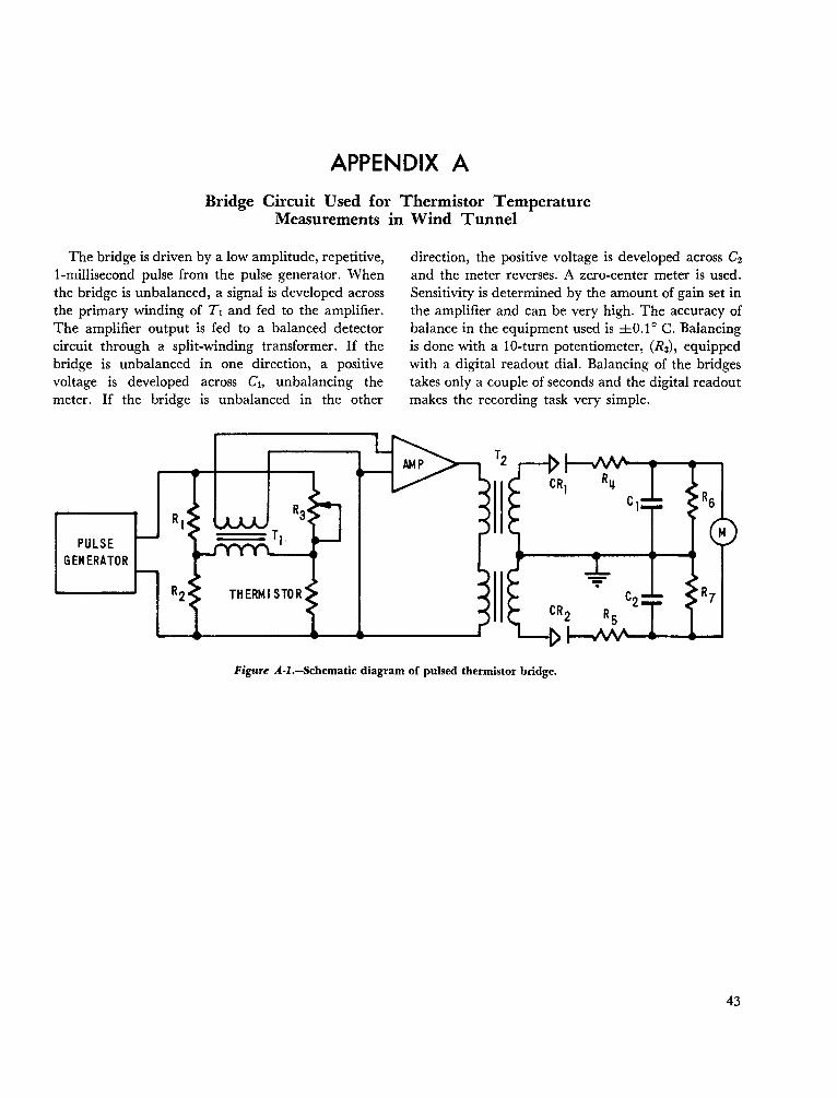
APPENDIX A

Bridge Circuit Used for Thermistor TemperatureMeasurements in Wind Tunnel

The bridge is driven by a low amplitude, repetitive,l-millisecond pulse from the pulse generator. Whenthe bridge is unbalanced, a signal is developed acrossthe primary winding of 7 1 and fed to the amplifier.The amplifier output is fed to a balanced detectorcircuit through a split-winding transformer. If thebridge is unbalanced in one direction, a positivevoltage is developed across Cr, unbalancing themeter. If the bridge is unbalanced in the other

direction, the positive voltage is developed across C2

and the meter reverses. A zero-center meter is used.Sensitivity is determined by the amount of gain set inthe amplifier and can be very high. The accuracy ofbalance in the equipment used is ±O.lo C. Balancingis done with a la-turn potentiometer, (Ra), equippedwith a digital readout dial. Balancing of the bridgestakes only a couple of seconds and the digital readoutmakes the recording task very simple.

RSR1

MPULSE

GENERATOR

R2 THERMI STOR R7

Figure A·I.-Schematic diagram of pulsed thermistor bridge.

43

APPENDIX B

Solution of Wave Tank Electrical Analog

The electrical analog for the wave tank experimentis given below.

The problem is to find the time function of thecharge on C2 after closing switch S. The theoreticalamplifier A in the diagram has infinite input im­pedance, zero output impedance, and unity gain.The perfect isolation of the amplifier then permitsus to solve the above circuit in two stages. First wesolve for the voltage on CI , then use this relationshipas the driving voltage for the second circuit involvingRa and C2•

Upon closing switch S we may write for the voltagearound the first loop

(B-l)

Rearranging terms and simplifying we have

RILet --- =r and RICI=r

R I+R2

Then equation (B-2) becomes

d2q 1 dq-+--=0dt2 rr dt

This equation has a solution of the form

q(t) =Ae-(t/rr)+B

Let us set the boundary conditions

(B-2)

(B-3)

where t=O, q=qo and

Then equation (B-1) becomes

Differentiating with respect to t

Thus A=qo-B and B=CVr.The final solution is then

q(t) = (qo-CVr)r(t/rT)+CVr

=qoe-(t/rT)+CVr(1-e-(t/rr»)

Dividing by CI we have

V(t) = Voe-(!/rr)+ Vr(l-e-(!/rr») (B-4)

We may now use equation (B-4) for the voltage

TANK WET BULB ASSEMBLY

Figure B·l.-Electrical analog of evaporation experiment.

45

applied to RaC2• Equating the voltages around thesecond loop we have

qowhere Vo= - and

C2

Dividing by Ra we have

dq + !L = qo r(t/rT)+ qm (1_e-(t/rr)) (B-S)dt Tm Tm Tm

Equation (B-S) may be integrated by using the inte­grating factor e(tfrm). Multiplying both sides ofequation (B-S) by e(t/rm) we have

qo-qm!qe(t/rm ) = -- e[t(rr-rm)/rrTml dtTm

q(t) = rT(qo- qm) e[t(rr-rn,)/rrTmle-(t/rm )

rT-Tm

+qm+Ke-(t/rm)

() rT(qo-qm) e-(t/rT)+ Ve-(t/rm)q t =qm+ It'rT-Tm

ranging terms we have

q(t) =qm+ (qO-qm)rT e-(t/rr)+ (qm-qO)Tme-(t/rm)rT-Tm rT-Tm

(B-8)

Equation (B-8) is the solution of the electrical circuitwhere q is the charge on the Capacitors C2•

Going to the tank experiment, q becomes thespecific humidity and the boundary conditions are

qo= equilibrium specific humidity at start ofexperiment

q.= saturation specific humidity at the watertemperature

qm = maximum specific humidity reached at t- 00

r=qm/q•.

The other terms in equation (B-8) become

T = actual time constant of experiment if no airleakage were present

Tm = time constant of wet bulb.

Equation (B-8) thus becomes the solution to theevaporation experiment. Adding (qm-qo) to bothsides of equation (B-8) and rearranging terms wehave

Taking qo to the left side of the equation and dividingthrough by (qm - qo) we have

and therefore

Equation (B-9) is in a normalized form where onlytime constants are important. The start time andend points do not displace the experimental curve ifthe time constants remain fixed. This form permitsmuch better comparison of the experimental results.

(B-6)

Apply boundary condition q(t) = qo when t = 0

(B-7)

Combining equations (B-6) and (B-7) and ar-

46

[q-qo] rT Tm1- -- = -- e-(t/rr) - -- e-(t/rm)

qm-qo rT-Tm rT-Tm(B-9)

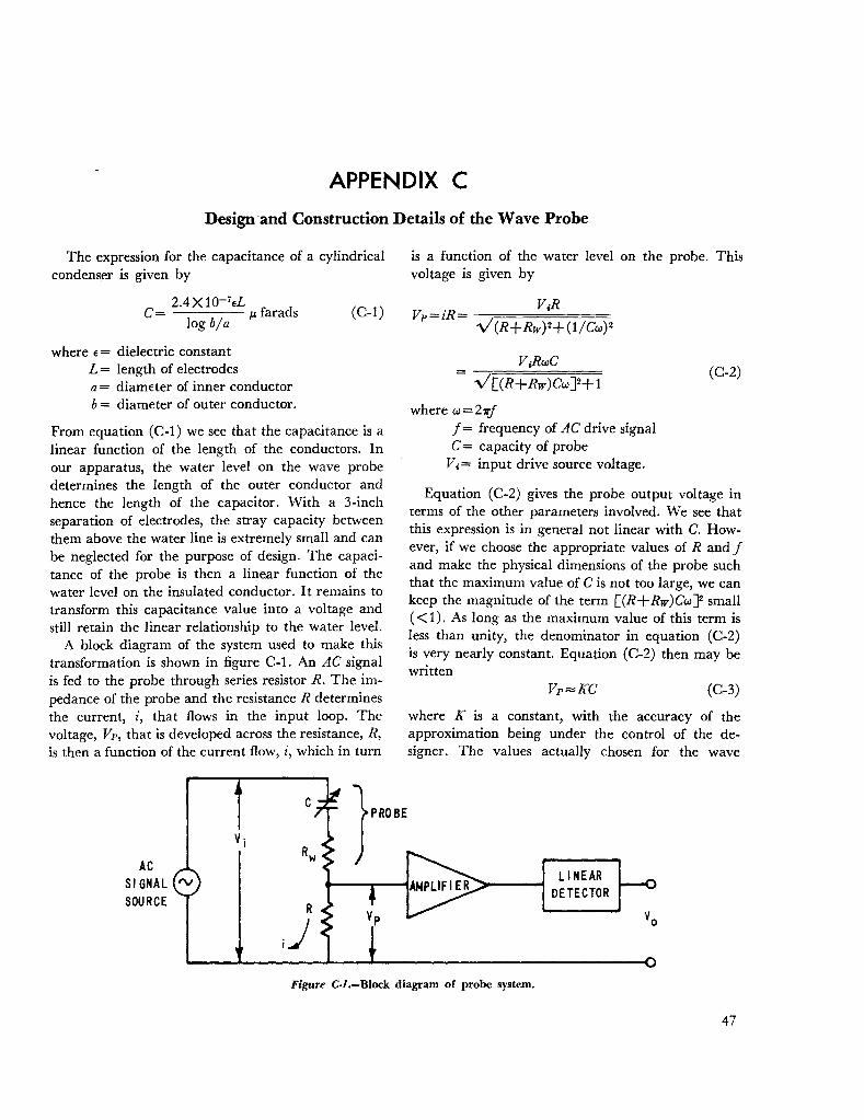
APPENDIX C

Design-and Construction Details of the Wave Probe

The expression for the capacitance of a cylindricalcondenser is given by

is a function of the water level on the probe. Thisvoltage is given by

2.4XI0-7ELc= / IJ. farads

log b a(C-l)

where K is a constant, with the accuracy of theapproximation being under the control of the de­signer. The values actually chosen for the wave

Equation (C-2) gives the probe output voltage interms of the other parameters involved. We see thatthis expression is in general not linear with C. How­ever, if we choose the appropriate values of Rand jand make the physical dimensions of the probe suchthat the maximum value of C is not too large, we cankeep the magnitude of the term [(R+Rw)CWJ2 small(<1). As long as the maximum value of this term isless than unity, the denominator in equation (C-2)is very nearly constant. Equation (C-2) then may bewritten

where E = dielectric constantL = length of electrodesa = diameter of inner conductorb= diameter of outer conductor.

From equation (C-l) we see that the capacitance is alinear function of the length of the conductors. Inour apparatus, the water level on the wave probedetermines the length of the outer conductor andhence the length of the capacitor. With a 3-inchseparation of electrodes, the stray capacity betweenthem above the water line is extremely small and canbe neglected for the purpose of design. The capaci­tance of the probe is then a linear function of thewater level on the insulated conductor. It remains totransform this capacitance value into a voltage andstill retain the linear relationship to the water level.

A block diagram of the system used to make thistransformation is shown in figure C-1. An AC signalis fed to the probe through series resistor R. The im­pedance of the probe and the resistance R determinesthe current, i, that flows in the input loop. Thevoltage, Vp , that is developed across the resistance, R,is then a function of the current flow, i, which in turn

VoRwC

where w=27rjj = frequency of AC drive signalC= capacity of probe

V.= input drive source voltage.

(C-2)

(C-3)

v·IAC

SI GNAL IV

SOURCE

LI NEARDETECTOR

Figure C-l.-Block diagram of probe system.

47

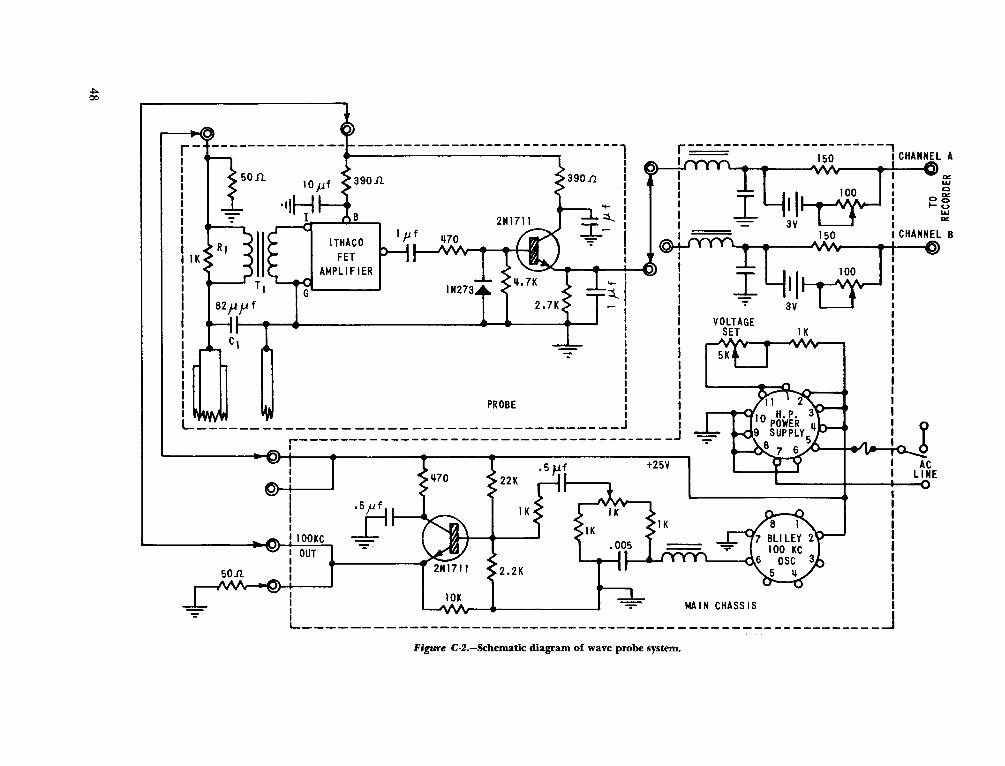
.j>..00

r:::::------------------,150 CHANNEL A./V'y , e

Q<....

II~ ~i3V' L..J - Q<

150 CHANNEL BM , 6)

II100

3VVOLTAGE

SET 1K~. . I 5K

1K

22K

2.2K

10K

----------------------;------,

B~

ITHACOFET

AMPLI FIER

OUT100KC

1... ~ MAIN CHASSIS I

-------------------------~

50n.

1K

L~ "" PROBE

------ -- r:':::=--:':':::::.:---=-:::::::.:.:-----::::::.: J

r-

Figure C-Z.-Schematic diagram of wave probe system.

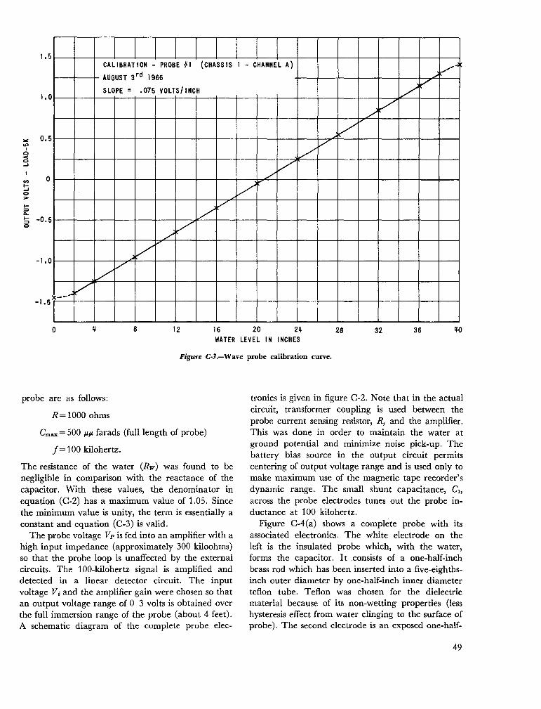
CALIBRATION - PROBE #1 (CHASSIS 1 - CHANNEL A) ~.... ...;

AUGUST 3rd 1966,/

SLOPE = .075 VOLTS/INCH V./

V

V./'"

V

./V

//

V

.//

/./'"

,/'

x--- /

o

1.0

0.5

-1.5

en::io:>

"'"'"IQc(o...J

1.5

-1.0

f­::>....!; -0.5o

o B 12 16 20 2qWATER LEVEL IN INCHES

28 32 36 qO

Figure C·J.-Wave probe calibration curve.

probe are as follows:

R=1000 ohms

Gmax = 500 /J.p. farads (full length of probe)

f = 100 kilohertz.

The resistance of the water (Rw) was found to benegligible in comparison with the reactance of thecapacitor. With these values, the denominator inequation (C-2) has a maximum value of 1.05. Sincethe minimum value is unity, the term is essentially aconstant and equation (C-3) is valid.

The probe voltage Vp is fed into an amplifier with ahigh input impedance (approximately 300 kiloohms)so that the probe loop is unaffected by the externalcircuits. The 100-kilohertz signal is amplified anddetected in a linear detector circuit. The inputvoltage Vi and the amplifier gain were chosen so thatan output voltage range of 0-3 volts is obtained overthe full immersion range of the probe (about 4 feet).A schematic diagram of the complete probe elec-

tronics is given in figure C-2. Note that in the actualcircuit, transformer coupling is used between theprobe current sensing resistor, R, and the amplifier.This was done in order to maintain the water atground potential and minimize noise pick-up. Thebattery bias source in the output circuit permitscentering of output voltage range and is used only tomake maximum use of the magnetic tape recorder'sdynamic range. The small shunt capacitance, GI ,

across the probe electrodes tunes out the probe in­ductance at 100 kilohertz.

Figure C-4(a) shows a complete probe with itsassociated electronics. The white electrode on theleft is the insulated probe which, with the water,forms the capacitor. It .consists of a one-half-inchbrass rod which has been inserted into a five-eighths­inch outer diameter by one-half-inch inner diameterteflon tube. Teflon was chosen for the dielectricmaterial because of its non-wetting properties (lesshysteresis effect from water clinging to the surface ofprobe). The second electrode is an exposed one-half-

49

Figure C-4.-Wave measuring probe.

inch brass rod. Figure C-4(b) shows a close-up of theprobe head. The two rods are threaded through a3- by 3-inch solid nylon block for strength and lowcapacitive strays. A brass box is sealed over the topof the nylon block and houses some of the associated

50

probe electronics. A rubber gasket around the faceplate of the box makes the whole probe head com­pletely water tight. In the field installation, theBNG connectors were "potted" in place with a siliconerubber compound.

APPENDIX DBasic Data From the Wave Tank Evaporation Experiments

v= average wind speed in the evaporation sec­tion of the tank in feet per second

H = average wave height (peak to trough) ininches

L = wave length in inchesT = wave period in seconds

H/L= wave height to length ratio (dimensionless)H/T= wave height to period ratio in inches per

second

r = time constant in seconds of experiment,computed from the semilog plots of thedata points

D= evaporation coefficient =v/Ar feet persecond where the tank parameter v/A =5.8feet.

NOTE: Where wave height H is indicated to be zero, smallwind-driven capillaries were present. However, no paddlegenerated waves were present.

Run No. V H L T HIL HIT T D DIV

32 8.34 0 ---------- ---------- ------------ ---------- 88 0.066 0.0079

33 6.20 0 ---------- ---------- ------------ ---------- 113 0.052 0.0084

34 4.16 0 ---------- ---------- ------------ ---------- 115 0.036 0.00865

35 2.92 0 ---------- ---------- ------------ ---------- 218 0.027 0.0093

36 10.0 6 120 1.84 0.050 3.26 80 0.073 0.0073

37 6.0 5 120 1.84 0.040 2.72 115 0.051 0.0085

38 4.16 5 120 1.84 0.040 2.72 133 0.044- 0.0106

39 2.92 5 120 1.88 0.040 2.72 160 0.036 0.0123

40 12.5 6 80 1.40 0.075 4.30 73 0.080 0.0064

41 8.3 6 80 1.40 0.075 4.30 101 0.058 0.0070

42 5.5 6 80 1.40 0.075 4.30 118 0.049 0.0089

43 3.8 6 80 1.40 0.075 4.30 133 0.044- 0.0116

44- 15.8 7.5 75 1.20 0.10 6.25 65 0.091 0.0058

45 10.0 8 60 1.44- 0.133 7.02 73 0.081 0.0081

46 5.0 8 60 1.1 0.133 7.28 82 0.072 0.0146

47 2.92 8 65 1.19 0.123 6.72 102 0.058 0.0200

48 9.0 3 160 2.35 0.019 1.27 80 0.074 0.0082

49 5.84 2.5 160 2.35 0.016 1.07 109 0.054 0.0096

50 3.0 2 160 2.35 0.013 0.085 162 0.037 0.0123

51 13.0 6 80 1.39 0.075 4.3 74 0.086 0.0066

52 9.0 6 80 1.39 0.075 4.3 97 0.064 0.0071

53 3.0 6 80 1.39 0.075 4.3 149 0.042 0.0140

54 3.0 6 80 1.39 0.075 4.3 158 0.037 0.0123

55 13.0 4 55 0.97 0.073 4.1 69 0.084 0.0065

56 10.8 4 55 0.97 0.073 4.1 84 0.069 0.0064

57 4.0 5 55 0.97 0.091 5.15 118 0.049 0.0122

58 8.3 3 145 2.1 0.021 1.43 84 0.069 0.0083

59 6.7 2 145 2.1 0.014 0.95 104 0.056 0.0084

60 2.5 2 145 2.1 0.014 0.95 188 0.031 0.0124

61 10.0 4 80 1.39 0.050 2.88 74 0.079 0.0079

62 8.3 4 80 1.39 0.050 2.88 88 0.066 0.0079

63 3.0 4 80 1.39 0.050 2.88 152 0.038 0.0126

64 13.3 6.5 60 1.06 0.110 6.13 75 0.078 0.0059

65 9.2 6 60 1.06 0.10 5.66 97 0.060 0.0065

66 3.5 6 60 1.06 0.10 5.66 136 0.043 0.0123

51

Run No. V H L T H/L H/T T D D/V

67 8.3 2 145 2.3 0.014 0.87 85 0.069 0.008368 6.0 2 145 2.3 0.014 0.87 112 0.052 0.008769 2.5 3.5 145 2.3 0.024 1.57 204 0.029 0.011670 10.0 3.5 80 1.33 0.044 2.64 78 0.075 0.007571 5.0 0 ---------- ---------- ------------ ---------- 114 0.051 0.010272 7.5 4 80 1.33 0.050 3.0 103 0.057 0.007673 2.5 4 80 1.33 0.050 3.0 180 0.032 0.012874 13.0 6 55 0.90 0.11 6.68 80 0.073 0.005675 8.3 6 55 0.90 0.11 6.68 98 0.059 0.007176 3.0 6 55 0.90 0.11 6.68 154 0.038 0.012677 14.0 4 50 0.83 0.08 4.83 69 0.084 0.006078 10.0 5 50 0.83 0.10 6.02 84 0.069 0.006979 3.5 4.5 50 0.83 0.090 5.4 118 0.049 0.014080 12.5 0 ---------- ---------- ------------ ---------- 65 0.089 0.007181 13.3 4 150 2.36 0.027 1.69 59 0.098 0.007482 14.0 4.5 120 I. 70 0.038 2.65 56 0.104 0.007483 17.0 6 85 1.39 0.071 4.30 53 0.110 0.006584 20.0 6.5 65 1.2 0.10 5.4 47 0.123 0.0061585 20.0 6.5 65 1.2 0.10 5.4 46 0.126 0.006386 12.5 4 150 2.41 0.027 1.66 56 0.104 0.008387 13.3 4 110 1. 70 0.036 2.35 58 0.10 0.007588 15.0 5.5 80 1.39 0.069 3.96 54 0.107 0.007189 20.8 6 60 1.0 0.1 6.0 48 0.121 0.005890 11.7 2 150 2.20 0.013 0.91 60 0.097 0.008391 12.5 3.5 120 1.61 0.029 2.18 58 0.100 0.008092 15.8 5 80 1.33 0.063 3.76 51 0.114 0.007293 20.8 6.5 60 1.0 0.11 6.5 51 0.114 0.005594 12.0 2 150 2.2 0.013 0.91 56 0.104 0.008795 12.5 2.5 120 I.70 0.021 1.47 62 0.094 0.007596 16.0 4.5 75 1.50 0.060 3.0 51 0.114 0.007197 18.4 6 60 1.11 0.10 5.4 50 0.116 0.006398 15.8 0 ---------- ---------- ----------- - ---------- 47 0.123 0.007899 15.8 3 150 2.12 0.020 1.42 50 0.116 0.0074

100 16.7 4 110 1.6 0.036 2.5 46 0.126 0.0076101 18.0 4 75 1.3 0.053 3.06 43 0.135 0.0075102 25.0 5.5 50 0.87 0.11 6.32 38 0.152 0.0061103 16.0 4 150 2.4 0.027 1.67 45 0.129 0.0081104 18.0 4 115 1.68 0.035 2.38 40 0.145 0.0081105 20.0 5.5 80 1.39 0.069 3.96 40 0.145 0.0073106 15.8 5.5 155 2.35 0.036 2.34 46 0.126 0.0080107 18.5 6 120 1.93 0.050 3.11 40 0.145 0.0078108 21.0 6 80 1.39 0.075 4.33 41 0.141 0.0067

I

52

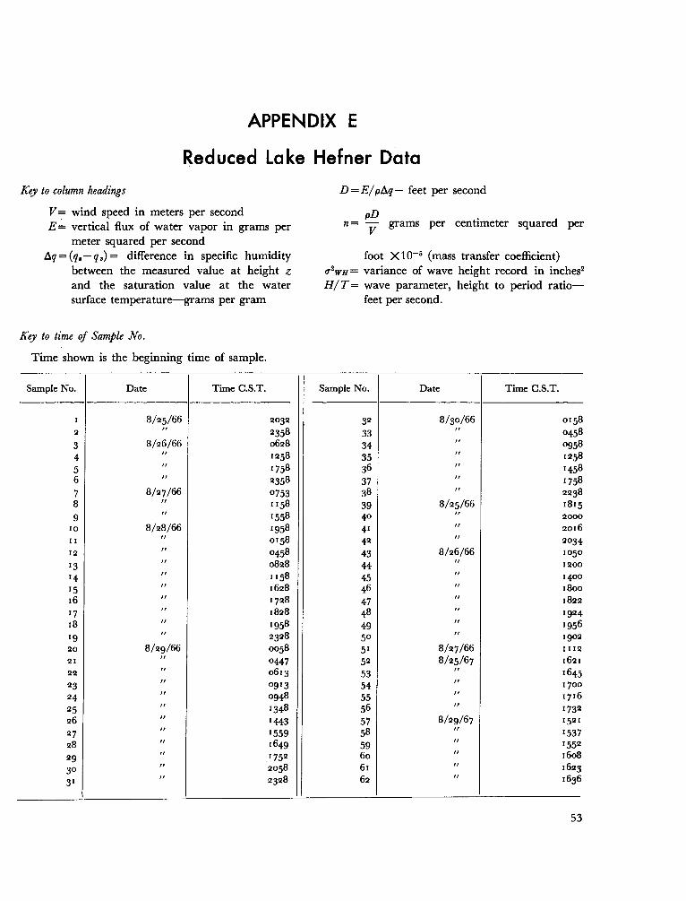
APPENDIX E

Red uced La ke Hefner Data

Key to column headings

V~ wind speed in meters per secondE= vertical flux of water vapor in grams per

meter squared per second~q= (q.-q.) = difference in specific humidity

between the measured value at height zand the saturation value at the watersurface temperature-grams per gram

Key to time of Sample No.

Time shown is the beginning time of sample.

D = E/p~q - feet per second

pD .n= V grams per centimeter squared per

foot X 10-5 (mass transfer coefficient)(J'2WH = variance of wave height record in inches2

H/T= wave parameter, height to period ratio­feet per second.

Sample No. Date Time e.S.T. Sample No. Date Time e.S.T.

I 8/25/66 2032 32 8/30/66 01 582 " 2358 33 " 04583 8/26/66 0628 34 " 09584 " 1258 35 " 12585 " 1758 36 " 14586 " 2358 37 " 17587 8/27/66 0753 38 " 22388 " 1158 39 8/25/66 18159 " 1558 40 " 2000

10 8/28/66 1958 41 " 2016II " 01 58 42 " 203412 " 0458 43 8/26/66 105013 " 0828 44 " 120014 " 1158 45 " 140015 " 1628 46 " 180016 " 1728 47 " 182217 " 1828 48 " 192418 " 1958 49 " 195619 " 2328 50 " 190220 8/29/66 0058 51 8/27/66 111221 " 0447 52 8/25/67 162122 " 061 3 53 " 164523 " 0913 54 " 170024 " 0948 55 " 171625 " 1348 56 " 173226 " 1443 57 8/29/67 152127 " 1559 58 " 153728 " 1649 59 " 1552

" 1752 60 " 160829" 2058 61 " 162330" 2328 62 " 163631

53

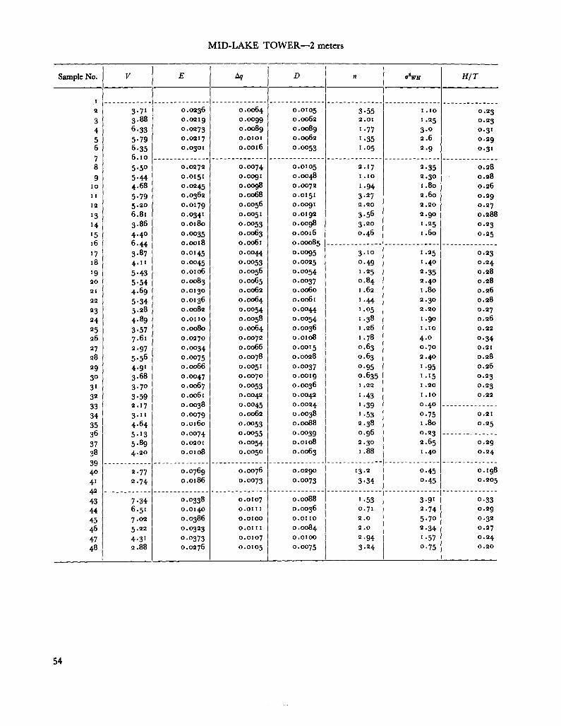
MID-LAKE TOWER-2 meters

Sample No. V E liq D n trwH HIT

I ------------ -------------- -------------- -------------- --- ----------- -------------- --------------2 3.71 0.0236 0.0064 0. 0105 3·55 1.10 0.233 3.88 0. 021 9 0.0099 0.0062 2.01 1.25 0.234 6'33 0.0273 0.0089 0.0089 1.77 3.0 0.315 5·79 0.021 7 0.0101 0.0062 1.35 2.6 0.296 6'35 0.0301 0.0016 0.0053 1.05 2·9 0.317 6.10 -------------- -------------- -------------- -------------- -------------- --------------8 5.50 0.0272 0.0074 0.0105 2.17 2·35 0.289 5·44 0.01 51 O.Oogl 0.0048 1.10 2.30 0.28

10 4.68 0. 0245 o.oogS 0.0072 1.94 1.80 0.26II 5·79 0.0362 0.0068 0.01 51 3. 27 2.60 0.2912 5.20 0. 01 79 0.0056 0.0091 2.20 2.20 0.2713 6.81 0.0341 0.005 1 0.0192 3.56 2.go 0.28814 3.86 0.0180 0.0053 o.oogS 3.20 1.25 0.2315 4.40 0.0035 0.0063 0.0016 0.46 1.60 0.2516 6,44 0.0018 0.0061 0.00085 -------------- -------------- --------------17 3.87 0.01 45 0.0044 0.0095 3. 10 1.25 0.2318 4. 11 0.0045 0.0053 0. 0025 0·49 1.40 0.2419 5·43 0.0106 0.0056 0.0054 1.25 2·35 0.2820 5·54 0. 0083 0.0065 0.0037 0.84 2.40 0.2821 4.69 0.01 30 0.0062 0.0060 1.62 1.80 0.2622 5·34 0.01 36 0.0064 0.0061 1·44 2.30 0.2823 5. 28 0.0082 0.0054 0.0044 1. 05 2.20 0.2724 4.89 0.0110 0.0058 0.0054 1.38 1.90 0.2625 3·57 0.0080 0.0064 0.0036 1.26 1.10 0.2226 7.61 0.0270 0.0072 0.0108 1.78 4. 0 0·3427 2·97 0.0034 0.0066 0.001 5 0.63 0.70 0.2128 5.56 0.0075 0.0078 0.0028 0.63 2.40 0.2829 4.91 0.0066 0.0051 0.0037 0·95 1.95 0.26

30 3.68 0.0047 0.0070 0.001 9 0.635 1.15 0.23

31 3.70 0.0067 0.0053 0.0036 1.22 1.20 0.23

32 3·59 0.0061 0.0042 0.0042 1.43 1.10 0.22

33 2.17 0.0038 0.0045 0. 0024 1.39 0.40 --------------

34 3. II 0.0079 0.0062 0.0038 1·53 0·75 0.21

35 4.64 0.0160 0.0053 0.0088 2.38 1.80 0.25

36 5. 13 0.0074 0.0055 0.0039 0.96 0.23 --------------

37 5.89 0.0201 0.0054 0.0108 2.30 2.65 0.29

38 4.20 0.0108 0.0050 0. 0063 1.88 1·40 0.24

39 ------------ .------------- --_.---------- -------------- -------------- -------------- --------------

40 2·77 0.0769 0.0076 0. 0290 13.2 0·45 O.lgS

41 2·74 0.0186 0.0073 0.0073 3·34 0·45 0.205

42 - -- --------- -------------- -------------- -------------- -------------- -------------- --------------

43 7·34 0.0338 0. 0107 0.0088 1.53 3.91 0·3344 6,51 0.01 40 0.01 I I 0.0036 0.71 2·74 0.29

45 7.02 0.0386 0.0100 0.0110 2.0 5.70 0.32

46 5.22 0.0323 0.0111 0. 0084 2.0 2·34 0.27

47 4.31 0.0373 0. 0107 0.0100 2·94 1.57 0.24

48 2.88 0. 0276 0. 0105 0.0075 3.24 0·75 0.20

---

54

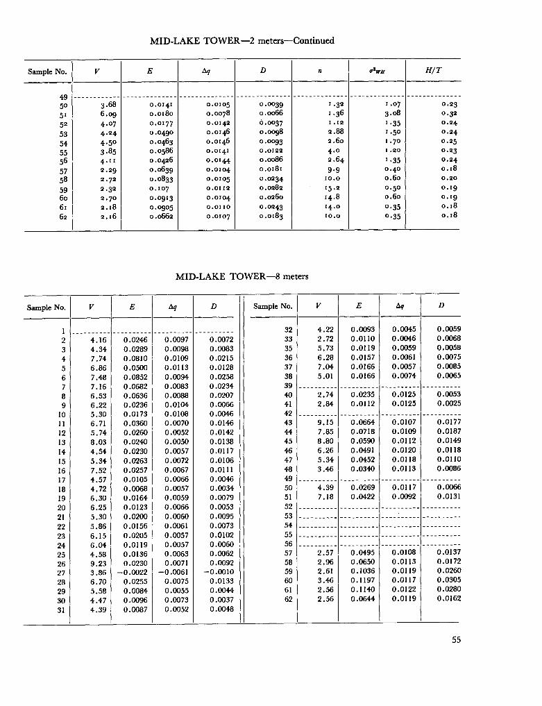
MID-LAKE TOWER-2 meters-Continued

Sample No. V E I!.q D n (l'IWH HIT

49 ------------ -------------- -------------- -------------- -------------- -------------- --------------50 3.68 0. 01 41 0.0105 0.0039 1.32 1.07 0.2351 6.09 0.0180 0.0078 0.0066 1.36 3.08 0.3252 4. 07 0. 01 77 0. 01 42 0.0037 1.12 1.35 0.24

53 4.24 0.0490 0.01 46 0.0098 2.88 1.50 0.24

54 4.50 0.0463 0.01 46 0·0093 2.60 1.70 0.25

55 3.85 0.0586 0.01 41 0.0122 4. 0 1.20 0.2356 4. 11 0,0426 0.01 44 0.0086 2.64 1.35 0.24

57 2.29 0. 0639 0.0104 0.0181 9·9 0.40 0.18

58 2.72 0.0833 0.0105 0.0234 10.0 0.60 0.20

59 2.32 0. 107 0.0112 0.0282 15.2 0.50 0.1960 2.70 0.0913 0.0104 0.0260 14.8 0.60 0.1961 2.18 0.0905 0.0110 0. 0243 14.0 0·35 0.1862 2.16 0.0662 0.0107 0.0183 10.0 0·35 0.18

MID-LAKE TOWER-8 meters

Sample No. V E Aq D Sample No. V E Aq D

I ---------- ---------- ---------- ---------- 32 4.22 0.0093 0.0045 0.0059

2 4.16 0.0246 0.0097 0.0072 33 2.72 0.01I0 0.0046 0.00683 4.34 0.0289 0.0098 0.0083 35 5.73 0.0119 0.0059 0.00584 7.74 0.0810 0.0109 0.0215 36 6.28 0.0157 0.0061 0.0075

5 6.86 0.0500 0.0113 0.0128 37 7.04 0.0166 0.0057 0.0085

6 7.48 0.0852 0.0094 0.0258 38 5.01 0.0166 0.0074 0.0065

7 7.16 0.0682 0.0083 0.0234 39 ---------- ---------- ---------- ----------8 6.53 0.0636 0.0088 0.0207 40 2.74 0.0235 0.0125 0.00539 6.22 0.0236 0.0104 0.0066 41 2.84 0.01I2 0.0125 0.0025

10 5.30 0.0173 0.0108 0.0046 42 ---------- ---------- ---------- ----------II 6.71 0.0360 0.0070 0.0146 43 9.15 0.0664 0.0107 0.017712 5.74 0.0260 0.0052 0.0142 44 7.85 0.0718 0.0109 0.018713 8.03 0.0240 0.0050 0.0138 45 8.80 0.0590 0.0112 0.014914 4.54 0.0230 0.0057 0.01I7 46 6.26 0.0491 0.0120 0.01I815 5.34 0.0263 0.0072 0.0106 47 5.34 0.0452 0.01I8 0.01I0

16 7.52 0.0257 0.0067 0.0111 48 3.46 0.0340 0.01l3 0.0086

17 4.57 0.0105 0.0066 0.0046 49 ---------- ---------- ---------- ----------18 4.72 0.0068 0.0057 0.0034 50 4.39 0.0269 0.01I7 0.006619 6.30 0.0164 0.0059 0.0079 51 7.18 0.0422 0.0092 0.0131

20 6.25 0.0123 0.0066 0.0053 52 ---------- ---------- ---------- ----------21 5.30 0.0200 0.0060 0.0095 53 ---------- ---------- ---------- ----------22 5.86 0.0156 0.0061 0.0073 54 ---------- ---------- ---------- ----------23 6.15 0.0205 0.0057 0.0102 55 ---------- ---------- ---------- ----------24 6.04 0.0119 0.0057 0.0060 56 ---------- ---------- ---------- ----------25 4.58 0.0136 0.0063 0.0062 57 2.57 0.0495 0.0108 0.0137

26 9.23 0.0230 0.0071 0.0092 58 2.96 0.0650 0.0113 0.0172

27 3.86 -0.0022 -0.0061 -0.0010 59 2.61 0.1036 0.01l9 0.0260

28 6.70 0.0255 0.0075 0.0133 60 3.46 0.1l97 0.0117 0.0305

29 5.58 0.0084 0.0055 0.0044 61 2.56 0.1l4O 0.0122 0.0280

30 4.47 0.0096 0.0073 0.0037 62 2.56 0.0644 0.01l9 0.0162

31 4. 391

0.0087 0.0052 0.0048

55

INTAKE TOWER-2 meters

Sample No. V E t.q D n q2WH HIT

1 3.37 0.0599 0.0084 0.0203 7.55 1.05 0.192 3.98 0.0534 0.0080 0.0190 6.04 1. 75 0.233 4.11 0.0532 0.0081 0.0186 5.70 2.0 0.244 6.30 0.1434 0.0094 0.0435 8.66 5.54 0.335 6.05 0.0685 0.0081 0.0243 5.05 5.28 0.326 6.89 0.0795 0.0046 0.0493 9.0 6.0 0.347 6.16 0.0624 0.0068 0.0202 5.3 5.41 0.338 5.63 0.0460 0.0067 0.0185 4.35 4.75 0.319 4.68 0.0365 0.0045 0.0233 6.25 3.03 0.27

10 3.95 0.0469 0.0063 0.0212 6.76 1. 75 0.2311 6.34 0.0628 0.0047 0.0381 7.55 5.60 0.3312 4.97 0.0603 0.0038 0.0452 11.4 3.65 0.2913 6.33 0.0298 0.0030 0.0283 5.6 5.60 0.3314 3.91 0.0310 0.0037 0.0241 7.73 1. 70 0.2315 4.38 0.0010 0.0030 0.0009 0.28 2.50 0.2616 5.57 -0.0031 0.0038 -0.0024 -------------- - -- ----------- --------------17 3.74- 0.0098 0.0028 0.0101 3.37 1.45 0.2118 4.41 0.0179 0.0024 0.0215 6.10 2.60 0.2619 5.75 0.0244- 0.0038 0.0183 4.0 4.90 0.3220 5.66 0.0214 0.0032 0.0191 4.25 4.80 0.3221 4.49 0.0150 0.0031 0.0138 3.86 2.70 0.2622 4.41 0.0188 0.0038 0.0141 4.03 2.60 0.2623 5.24 0.0109 0.0025 0.0124 2.95 4.20 0.3024 4.91 0.0140 0.0026 0.0154 3.9 3.50 0.2825 3.94 0.0132 0.0036 0.0105 3.34 1. 70 0.2326 7.42 0.0232 0.0061 0.0109 1.86 6.27 0.3427 1.83 0.0056 0.0026 0.0063 4.30 0.35 --------------28 4.61 0.0256 0.0035 0.0212 5.68 2.85 0.2729 4.03 0.0054 -------------- -------------- ---------- - - -- 1.90 0.2330 3.53 0.0330 0.0046 0.0204 7.28 1.25 0.2031 4.18 ------ -------- -------------- -------------- ---------- - - -- 2.20 0.2432 4.16 0.0139 0.0036 0.0011 3.30 2.10 0.2433 2.00 0.0051 0.0030 0.0049 3.06 0.40 --------------34 3.77 0.0165 0.0030 0.0158 5.28 1.20 0.2235 3.56 -0.0006 0.0030 -0.0006 -------------- 1.06 0.2036 4.61 0.0021 0.0046 0.0013 0.54 2.90 0.2637 5.71 0.0147 0.0034 0.0124 2.74 4.90 0.3238 4.13 0.0493 0.0037 0.0383 11.7 2.05 0.2439 4.25 0.0512 0.0107 0.0137 4.05 2.36 0.24540 3.86 0.0537 0.0103 0.0148 4.95 1.42 0.21141 3.78 0.0711 0.0104 0.0194 6.60 1.56 0.22242 3.59 0.0576 0.0107 0.0153 5.35 1.29 0.20643 8.20 0.1040 0.0099 0.0300 4.53 6.22 0.32444- 6.05 0.0781 0.0092 0.0241 4.95 5.12 0.31545 6.78 0.0823 0.0080 0.0292 5.36 5.70 0.32346 6.23 0.0597 0.0081 0.0212 4.12 5.95 0.33847 5.56 0.0815 0.0078 0.0300 6.60 5.10 0.32048 4.51 0.0407 0.0073 0.0160 4.54 3.16 0.27649 4.21 0.0496 0.0045 0.0318 9.45 2.07 0.237

56

INTAKE TOWER-8 meters

Sample No. V E t.q D

1 4.29 0.0740 0.0074 0.02872 4.73 -0.0157 0.0089 -0.00513 4.72 0.1141 0.0088 0.03704 7.41 0.1580 0.0083 0.05535 7.28 0.1040 0.0070 0.04326 8.08 0.1328 0.0043 0.08907 6.70 0.08H 0.0064 0.03758 6.85 0.0664 0.0072 0.02629 5.85 0.0604 0.0053 0.0328

10 4.99 0.0550 0.0042 0.037311 7.50 0.0653 0.0047 0.039412 5.95 0.0417 0.0042 0.027913 7.49 0.0366 0.0034 0.030514 4.69 0.0287 0.0033 0.025015 5.25 0.0059 0.0030 0.005716 6.75 0.0383 0.0037 0.029817 4.65 0.0182 0.0024 0.021818 5.42 0.0179 0.0029 0.017819 6.68 0.0426 0.0030 0.040520 6.56 0.0410 0.0034 0.03H21 5.32 0.0222 0.0030 0.021122 5.08 0.0382 0.0035 0.031123 6.12 0.0295 0.0025 0.033724 5.74 0.0246 0.0024 0.029525 4.83 0.0076 0.0031 0.007126 8.67 0.0206 O.OOH 0.013527 2.47 0.0052 0.0039 0.003628 5.90 0.0399 0.0042 0.027329 5.16 0.0056 ---------- ----------30 3.81 0.0182 0.0044 0.011831 3.99 0.0292 0.0038 0.021932 4.11 0.0192 0.0031 0.017733 2.35 0.0066 0.0035 0.0053534 4.25 0.0253 0.0026 0.028035 3.47 -0.0874 0.0034 -0.073336 4.91 0.0005 0.0039 0.000437 6.73 0.0205 0.0037 0.002438 4.31 0.0311 0.0039 0.022739 4.74 0.0458 0.0100 0.013240 4.31 0.0794 0.0087 0.025941 4.32 0.0707 0.0089 0.022542 4.02 0.0758 0.0079 0.027243 9.17 0.0310 0.0072 0.0124H 6.81 0.0891 0.0094 0.026945 7.72 0.07H 0.0083 0.07H46 7.04 0.0798 0.0079 0.079847 6.28 0.1076 0.0076 0.107648 5.0 0.0671 0.0069 0.067149 4.50 0.0353 0.0070 0.0353

57

ABSTRACT

The evaporation rate from a water surface is shownto be greatly affected by surface waves in laboratoryand field tests. Laboratory experiments were madeusing a large wave tank-wind tunnel apparatus inwhich both wind speed and wave parameters couldbe controlled. The apparatus simulates wave condi­tions on large bodies of water with fetches up to amile or more. Tank experiments indicate certaincombinations of wind speed and well-developed wavesproduce an evaporation rate lower than the rateunder similar wind conditions with no waves present.Investigations of air flow over the waves show that,as wave heights increase, regions of dead air are ob­served leeward of wave crests, and vortices appear inthe wave troughs. The partially trapped air appar­ently forms an effective barrier to the vertical trans­port of water vapor. Wave and evaporation measure-

58

ments at Lake Hefner, Oklahoma, were very similarto the laboratory measurements. The Lake Hefnerdata were adjusted to previously measured evapora­tion coefficient relationships derived from water andenergy budget measurements. The resulting evapora­tion coefficient curve is believed to give an improvedmeasure of the instantaneous evaporation rate fromLake Hefner under given conditions for wind speed,water surface temperature, and ambient humidity.DESCRIPTORS-*evaporation/evaporation control/waves / *waves (water) / wind tunnels / wind veloc­ity / wind speed / water vapor / water temperature /*reservoir evaporation / lakes / laboratory tests / fieldinvestigations.IDENTIFIERs-*evaporation coefficient / evapora­tion tanks / Lake Hefner, Okla. / wave tanks / *waveheight / mass transport.

'" u.•. GOVERNMENT PRINTING O....ICE' 1- o-33lI-U4