AbstractThis paper studies the interplay between central and local governments in defining the optimal degree of decentralization in terms of public goods supply. The choice between full centralization and asymmetric decentralization implies a trade-off between the possibility to provide public goods at a lower cost, wherever this is pos-sible by decentralizing, and the possibility to fully internalize spillovers by full cen-tralization. We find that asymmetric decentralization introduces distortions into the public decision-making process. We also demonstrate that the power to interfere in the central government’s ruling mechanisms should be reduced for the jurisdictions that have decentralized, in order to make their decentralization choice convenient even for the citizens in the less efficient jurisdictions. Finally, we find the conditions under which asymmetric decentralization can be simultaneously advantageous for both rich and poor regions through the design of appropriate equalization transfers.
Keywords Public goods · Asymmetric decentralization · Intergovernmental relations · Equalization transfers · Positive political economy
1 Department of Economics and Social Sciences, Marche Polytechnic University, Ancona, Italy2 Dipartimento di Scienze Dell’Economia, Università Del Salento, Complesso Ecotekne, Strada
per Monteroni, Lecce 73100, Italy3 Department of Economics and Law, Sapienza University of Rome, Via del Castro Laurenziano
9, 00161 Rome, Italy4 Governance and Economics Research Network, Vigo, Spain
According to the traditional literature on federalism (Oates 1972), the choice between decentralization and centralization depends on the trade-off between the internalization of inter-jurisdictional spillovers (doing better by a national government) and the local information advantages (exploiting better by a sub-national government). However, with the second-generation theory of federal-ism more attention has been paid to the fiscal and political incentives facing sub-national policy-makers (Oates 2005; Weingast 2009). This would also affect the above mentioned trade-off and, in particular, the intergovernmental relationship between the centre and the local units.
More generally, the decision to allocate policy jurisdictions to different lev-els of government is related to a number of trade-offs between the advantages and disadvantages of centralized versus decentralized provision (Tommasi and Weinschelbaum 2007). For instance, the central government could discriminate unfairly between regions and choose to favour one region for political reasons (e.g., that with the top-ranking member of government comes from), thus justify-ing an institutional reform towards decentralization (Zantman 2002). In a similar fashion, the allocation of responsibility could differ systematically across local entities (or states) as it would never be optimal to allocate such responsibility uniformly among all of them (Jack 2004). Put differently, in some states/regions the responsibility, combined with the autonomy, for services delivery should rest, for instance, with the central government, while in other states/regions it should reside with the state/regional government. Moreover, when income differs sub-stantially across regions, centralization could be not always efficient as regional specificities may prevail leading to forms of partial fiscal federalism (Cerniglia et al. 2019). Overall, this could give rise to some new institutional settings, char-acterized by asymmetric degrees of decentralization due to the attitude/intention of either the central or the regional government. In fact, if one looks at some recent cross-country experiences, this seems to be the case.
For example, in Italy after the constitutional reform in 2001, the article 116 (third paragraph) of the Constitution introduces the possibility for Italian regions to request the attribution of additional forms and particular conditions of autonomy. This differentiated autonomy can be attributed at the claim of the region concerned, after consultation with the local authorities, with a state law approved by an abso-lute majority of the members, on the basis of agreement between the State and the Region concerned (Eupolis 2017; Zanardi 2017). In recent years, the request for greater autonomy has been put forward by nine regions (Lombardy, Veneto, Emilia-Romagna, Piedmont, Liguria, Tuscany, Marche, Umbria and Campania) and in two of them, i.e. Lombardy and Veneto, a referendum was held in 2017, which confirmed such request by citizens, anticipating the negotiations with the central government. By contrast, Emilia–Romagna directly committed the Governor of the Region to start negotiations with the State in the same year (Rizzo and Secomandi 2019).
In Spain, once the constitutional process was accomplished, 17 autonomous communities emerged and a highly asymmetric quasi-federal system was the
Economia Politica (2021) 38:625–656626
1 3
outcome (Keating 2000; Flynn 2004). This was mostly due to the increasing lev-erage acquired by the Catalan, Basque and a few other, autonomous governments at the negotiating table (Conversi 2007).1
In some cases, the sub-national autonomy is, however, less related to fiscal decen-tralization and much more to regulatory decentralization as in the Russian institu-tional system (Libman and Rochlitz 2019), where the Russian regions systematically passed laws and legal acts that often explicitly contradicted federal regulations, lead-ing to a “war of laws” (Lapidus 1999; Libman 2010). In this context, some regions managed to negotiate a higher level of autonomy from the center on a bilateral basis, leading to a highly asymmetrical design of Russian federalism (Hughes 2001; Mar-tinez-Vazquez 2007).
Finally, in other cases the central control has never declined to a level that allowed a comparable level of institutional variation at the sub-national level such as in China (Libman and Rochlitz 2019). For instance, under Mao China’s destiny was very much decided by what happened at the center, with the autonomy of regional and local states remaining extremely limited. However, Chinese sub-national gov-ernments gained over time a residual claim on revenues, which allows them to retain some of the resources generated in the region. This contributes to explain why Chi-nese regions feature higher growth incentives for regional officials. More generally, Chinese provinces enjoy a significant level of autonomy with respect to economic policy, which is why China can be seen as a de facto federation, although de jure the country is a unitary state.
Those different countries’ experiences seem to suggest that asymmetric arrange-ments within the decentralization architecture are more frequent and, in some cases, more accommodative, durable and practical, being also more flexible and effective in managing and preventing intergovernmental conflict (MacGarry 2001; Coakley 2004; Conversi 2007). Put differently, for the most part asymmetric decentralization within modern states could reflect agreements and the result of a voluntary exchange between regional and central governments, rather than wars of conquest or threats of secession, to manage successfully multilevel governance (Congleton et al. 2003; Congleton 2006).
However, some side effects and distortions may arise when asymmetric forms of decentralization take place within a single country, especially in terms of free-riding attitude by some regions that call for some corrective action from the centre. Recall-ing the theory of public choice from its origins (Buchanan and Tullock 1962; Tol-lison and Buchanan 1972), we could say that a State functioning could be adversely affected by the presence of too many special interests (usually causing an excessive growth in public spending).
In this paper, we try to shed some light on this issue starting with a default scenario characterized by an entirely centralized supply of a local public good. However, local governments may require the decentralization of this supply. In
1 In recent years, after a popular referendum in 2006 a new Statute of Autonomy granted self-govern-ment to Catalonia, including the possibility of separate membership in the UNESCO, further increasing Spain’s asymmetrical disposition.
Economia Politica (2021) 38:625–656 627
1 3
particular, we focus on the case in which decentralization occurs asymmetrically. Asymmetric decentralization can take place for different reasons. For example, because the citizens have different preferences at the local level, or because some local governments are in a better position concerning their cost structrure, i.e. they can provide the public good at lower costs than the central government. The latter case is discussed in our study. Thus, if asymmetric decentralization is possible only for the most efficient local governments, the provision of local public policies in less efficient jurisdictions will remain a central government’s responsibility.
The tax base used to finance the public policies in the territories that have obtained decentralization will be separated from the central budget. In this context, we study the spillover effects generated by asymmetric decentralization and the free-riding incentives introduced by the former. The choice between full centralization and asymmetric decentralization implies a trade-off between the possibility to pro-duce at a lower cost, wherever this is possible by decentralizing, and the possibility to fully internalize spillovers by full centralization. In this framework, understanding how and to what extent asymmetric decentralization can improve welfare is not a trivial task.
Furthermore, we claim that asymmetric decentralization introduces distortions in the public decision-making process, whose consequences require an adequate under-standing for both governments and voters. The jurisdictions that obtain decentrali-zation can decide their public goods supply and, at the same time, they contribute to define public policies that the central government will implement in the other non-decentralized regions. We demonstrate that the power to interfere in the central government’s decision-making process should be reduced for the jurisdictions that have decentralized in order to make their decentralization choice convenient even for the citizens in the less efficient jurisdictions.
Finally, to enrich the analysis and make it closer to the real-world experience, we relax the assumption of no inter-regional differences in the per capita income, also including an equalization transfer mechanism. Accordingly, we are able to ana-lyse the regional disparities in the level economic development as one of the main arguments that has traditionally contributed to explain the local demand for greater autonomy (Mangiameli et al. 2020). This extension complements the assump-tion of territorial specific costs (e.g., due to morphology, urban concentration, and other exogenous factors), which are independent of the governments’ quality and institutional responsibility of public goods provision. In fact, the choice between, for instance, full centralization and asymmetric decentralization might be also determined by the existence of inter-regional income disparities that call for inter-regional fiscal flows, which can play an important role in this story. Looking at some countries’ experience (e.g., Belgium, United Kingdom, Spain, Canada, Germany), it can be noted that even though some forms of territorial gap exist—between the North and the South; the East and the West—, the institutional asymmetry did not worsen the regional divide as it has been complemented by equalization tools that made that divide less severe. This paper finds the conditions under which asym-metric decentralization can be simultaneously advantageous for both rich and poor regions through the design of appropriate equalization transfers.
Economia Politica (2021) 38:625–656628
1 3
The paper proceeds as follows. Section 2 develops the economic framework. Sec-tions 3 to 5 study equilibrium polices under full centralization, full decentralization and asymmetric decentralization, respectively. Section 6 shows the welfare implica-tions in the different institutional settings. Section 7 discusses the role of veto power in the decision to decentralize, while Sect. 8 provides an extension of the baseline model including income heterogeneity among regions. Finally, Sect. 9 concludes. The Appendix contains derivations and proofs of the propositions.
2 The economy
We use a framework similar to that of Besley and Coate (2003) and Giuranno (2009, 2010). In detail, we consider two equal sized jurisdictions comprising a federation and normalize to one the population of each jurisdiction. In the economy two kinds of goods are considered: a public one, g, and a private one, y; the former refers to some public provision aimed at fulfilling collective interest (e.g., control of environ-mental pollution), while the latter represents the personal income to be consumed for private purposes as well as to finance the public good.
Citizens are all alike; that is, they are endowed with the same income and have the same taste � regarding the public good. The parameter 𝜆 > 0 tells us how much citizens value g with respect to y.
Citizens vote in order to elect their delegates to act either in the central govern-ment or in the regional government. Since citizens are all alike, any of them can represent the constituency. The preferences ui of the representative of jurisdiction i are given by the following equation:
The parameter k ∈[
0, 1∕2]
measures the degree of spillovers, which is the same for all citizens; when k = 0 citizens care only about the public good provided in their own jurisdiction, while when k = 1∕2 they benefit equally about the public good in both jurisdictions (Besley and Coate 2003). The term (1 − ti)y denotes after tax income available for private consumption, where y is the pre-tax income and ti is the tax rate in jurisdiction i. Note that the condition gi ≥ 1 means that a minimal level of public good must be provided by default.
We assume that the cost of public good production is different if the public good is provided either by the central or the local governments. Such difference could be due to different administrative skills and knowledge between local and central officials, bureaucrats and policy-makers. Indeed, local government could better minimize political transaction costs by promoting, for instance, the transfer of cer-tain services and maintaining in-house production for others (Williamson 1985). In this way, local officials can concentrate on potential productive and allocative efficiency gains, also better controlling performance and attending to service dis-ruptions (Tavares and Camöes 2007). The opposite could also be true, that is local government’s action could be easily distorted by lobbyist pressures and even by the
(1)ui = (1 − ti)y + �[
(1 − k) ln gi + k ln g−i]
, with i = 1, 2 and gi ≥ g = 1.
Economia Politica (2021) 38:625–656 629
1 3
infiltration of organized crime (Ravenda et al. 2020). Such differences depend on the quality of institutions, thus when the spending allocation among levels of govern-ments change also the costs of public good provision change.2
In particular, we assume that 0 < c1 < c < c2 , where c1 , c and c2 are the unit costs of production in region 1, at the central level and in region 2, respectively. Hence, we define region 1 as the efficient one and region 2 as the inefficient one. Further-more, we assume that c, c1 and c2 are common knowledge.
Note that such cost structure includes the cases of different economies of scale. Indeed, if c < c1+c2
2 we have economy of scale because of costs subadditivity; when
c >c1+c2
2 , we have diseconomy of scale. There is no scale economy if c = c1+c2
2 ; in
this case, the unit cost of the central government is simply the average cost c = c1+c2
2.3
In what follows we consider three alternative scenarios: (1) the public good g is set by the central government under full centralization; (2) policy g is set under full decentralization; (3) policy g is set under asymmetric decentralization, where one jurisdiction can define policy g under decentralization, while the other jurisdiction cannot.
3 Policy determination under full centralization
We assume that under full centralization the central government adopts a uniform policy across jurisdictions; that is, gi = gC . Furthermore, policy is chosen by nego-tiation under the threat that, in the case of disagreement, it cannot be set by regional governments.4
The centralized budget is
The agreement utility is
While, the disagreement utility is y − c , the income minus the cost for producing the minimum provision of public good.5 Note that under centralization spillovers are fully internalized (Besley and Coate 2003).
(2)2cgC = 2ty ⇒ t =cgC
y.
(3)y − cgC + � ln gC.
3 In Sect. 8, we relax the assumption of c1< c < c
2 admitting very large economies of scale, i.e. c < c
1.
4 See Biswas and Giuranno (2019) and Giuranno (2009).5 Note that we assume that a minimum level of public good gC is always guaranteed; that is, gC can be seen as a merit good. Furthermore, without loss of generality, we set the default value of gC to unity, which also ensures an always weakly positive value of ln gC.
2 However, for the provision of many public goods, differences in costs depend only on the objective characteristics of regions. In this case, the cost for providing public goods in a region does not change when the providing government changes. We address the case of regional specific costs, as opposed to institutional specific costs, in Sect. 8.
Economia Politica (2021) 38:625–656630
1 3
We show the central government’s policy outcome as the solution of Nash bar-gaining between jurisdictional representatives; that is,
where, � = −c(gC − 1) + � ln gC ≥ 0 is the net gain of each representative from reaching an agreement on policy gC . Note that a necessary condition for � ≥ 0 is that � ≥ c ; that is, equilibrium net gains are weakly positive when citizens value the public good highly enough. In the latter case, the default value gC = 1 is suboptimal and an agreement on the supply of a gC ≥ 1 is achieved.
Centralized policy outcome is
As a result, regardless of where citizens live, individual welfare under full centrali-zation is
4 Policy determination under full decentralization
Under full decentralization, jurisdictions set policy at local level independently from each other and according to their budget constraint. The latter is given by
Decentralized Nash equilibrium is the solution to the following problem:
Solutions are:
Solution in Eq. 6 leads to the following Proposition.6
Proposition 1 Under full decentralization, spillovers are not internalized. Further-more, the jurisdiction that produces at a lower cost than the central government can compensate the loss due to the spillover through a lower production cost, while the
gC = argmax�2,
(4)gC =�
c, which implies tC =
�
y.
(5)uC = y − � + � ln�
c.
tDi=
cigDi
y, with i = 1, 2.
gDi= argmax
{
y − cigDi+ �
[
(1 − k) ln gi + k ln g−i]}
, with i = 1, 2.
(6)gDi=
�(1 − k)
ciand tD
i=
�(1 − k)
y, with i = 1, 2.
6 Note that solution (6) exists if and only if 𝜆 >ci
1−k . Furthermore, a sufficient condition in order to have
gDi≥ 1 ∀ k ≤ 1∕2 is � ≥ 2c
2.
Economia Politica (2021) 38:625–656 631
1 3
jurisdiction with a higher production cost always provides a lower level of public good than that of the central government.
When we compare full decentralization with full centralization, we find that pub-lic goods provision is underprovided by an amount (1 − k) in both jurisdictions. Fur-thermore, the following relations hold: gD
2< gC ; gD
2< gD
1 ; gD
1⋚ gC ; tD
1= tD
2≤ tC .
Against a uniform tax rate, the inefficient jurisdiction will certainly reduce public good provision under decentralization. Instead, policy outcome in the efficient juris-diction can be either higher or lower than that under full centralization. Thus, only the efficient jurisdiction can compensate the decentralized loss due to the spillover effect through a lower production cost. Clearly, the inefficient region prefers full centralization to full decentralization because it can benefit from both a lower cost and the internalized spillovers. While, the region that produces at a lower cost than the central government prefers to use its own technology, provided the gain of a lower cost, more than to compensate the loss due to not internalizing spillovers.
Furthermore, according to solution (Eq. 6), individual welfare under full decen-tralization is
5 Policy determination under asymmetric decentralization
In this section, we analyse the case of asymmetric decentralization. We assume that when a jurisdiction is more efficient then the central government in providing the public good it may obtain the power to set policy autonomously at the decentralized level.
Recalling that we have assumed that jurisdiction 1 is more efficient then the cen-tral government in the provision of the public good g, while jurisdiction 2 does not, only jurisdiction 1 will be able to obtain the decentralization of public good provi-sion. In that case, policy is chosen and implemented at the decentralized level for jurisdiction 1 and at the centralized level for jurisdiction 2.
It should be noted that asymmetric decentralization is not a secession since there is no a complete separation from the federation and no region does leave the national state. Indeed, even the more efficient region has an incentive to remain and to bar-gain on the national decision-making process regarding public good provision in the other region as it is interested in the internalization of externalities.
First, we study the policy choice of jurisdiction 1 that can decentralize; that is, jurisdiction 1 sets gA
1 as follows:
(7)
uDi= y − cig
Di+ �
[
(1 − k) ln gDi+ k ln gD
−i
]
= y − �(1 − k) + �
[
(1 − k) ln�(1 − k)
ci+ k ln
�(1 − k)
c−i
]
= y − �(1 − k) + �
[
ln (1 − k) + (1 − k) ln�
ci+ k ln
�
c−i
]
, with i = 1, 2.
Economia Politica (2021) 38:625–656632
1 3
that is,
The equilibrium policy of jurisdiction 1 is
Therefore, jurisdiction 1 sets policy at the decentralized level without internalizing the spillovers produced on the other jurisdiction. Furthermore, in equilibrium, juris-diction 1 chooses exactly the same policy that it would choose under full decentrali-zation, i.e. gA
1= gD
1.
Instead, in jurisdiction 2 public good provision is chosen by bargaining at the central level between the representatives elected in the two jurisdictions. Since the central government’s budget constraint excludes the tax revenues collected in juris-diction 1, it is given by
where, the centralized tax rate tA = tA2 is levied only on the tax base of the jurisdic-
tion that has to receive the central government provision, since jurisdiction 1 uses its tax base for financing its own provision.
The agreement utility of the representative of jurisdiction 1 is
Under disagreement, the central government cannot provide the public good in juris-diction 2 above the minimum guaranteed level, which is 1 by assumption. Therefore, the disagreement utility for the representative of jurisdiction 1 is given by
The net gain from reaching an agreement over public good provision in jurisdiction 2 must be weakly positive for the jurisdictional representatives. The net gain for the representative of jurisdiction 1 is
Note that 𝜕𝜓1∕𝜕gA2> 0 ; that is, the efficient jurisdiction is interested in the highest
possible centralized provision in the inefficient jurisdiction in order to benefit from its spillover as much as possible.
gA1= argmax
{
y(
1 − tA1
)
+ �[
(1 − k) ln gA1+ k ln gA
2
]}
, s.t. c1gA1= tA
1y;
gA1= argmax
{
y − c1gA1+ �
[
(1 − k) ln gA1+ k ln gA
2
]}
.
(8)gA1=
�(1 − k)
c1and tA
1=
�(1 − k)
y.
cgA2= tA
2y ⇒ tA
2=
cgA2
y
(9)uA1= y
(
1 − tA1
)
+ �[
(1 − k) ln gA1+ k ln gA
2
]
= y − c1�(1−k)
c1+ �
[
(1 − k) ln�(1−k)
c1+ k ln gA
2
]
.
uAd
1= y
(
1 − tA1
)
+ �(1 − k) ln gA1
= y − c1�(1−k)
c1+ �(1 − k) ln
�(1−k)
c1.
(10)�1 = uA1− uA
d
1= �k ln gA
2≥ 0.
Economia Politica (2021) 38:625–656 633
1 3
Instead, for jurisdiction 2, the agreement utility is
Note that by maximizing Eq. (11) with respect to gA2 , we obtain the first best of juris-
diction 2 when policy is chosen by the central government by using its technology; that is,
Equation (12) can be seen as the utopia point of jurisdiction 2, which defines the maximum possible achievement of public good provision that jurisdiction 2 may reach in the bargaining situation. Thus, this amount in asymmetric decentralization (Eq. 12) is always higher than that provided under full decentralized (Eq. 6) and lower then that provided under full centralization (Eq. 4).
The disagreement utility for jurisdiction 2, which implies gA2= 1 , is
The net gain for the representative of jurisdiction 2 is given by
It is worth studying policy outcome in the absence of spillovers ( k = 0 ) before focus-ing on the case where k ≠ 0 . This allows us to define a benchmark result expressed in the following Proposition.
Proposition 2 In the absence of spillover ( k = 0 ), asymmetric decentralization gen-erates the highest possible welfare for all jurisdictions.
When k = 0 , the net gain (Eq. 10) of jurisdiction 1 from policy provision in jurisdiction 2 is null. This means that jurisdiction 1 is indifferent to the level of gA
2
decided by the central government. Therefore, jurisdiction 2, which has a positive net gain (Eq. 13) even when k = 0 , will be able to obtain the preferred level of provision in the central government since jurisdiction 1 has no incentive to oppose. As a result, it is straightforward to verify that when k = 0 policy outcome in the two jurisdictions is given by gA
1=
�
c1 and gA
2= gFB
2=
�
c , where gA
1> gA
2 since
c1 < c . Asymmetric decentralization is always weakly welfare improving for all jurisdictions since they can benefit from higher public good provision at lower costs. In detail, consider that the following relations hold when k = 0 : gA1= gD
1> gC ; gA
2= gC > gD
2 ; uA
1= uD
1> uFC ; uA
2= uFC > uD
2.
(11)uA2= y
(
1 − tA)
+ �[
(1 − k) ln gA2+ k ln gA
1
]
= y − cgA2+ �
[
(1 − k) ln gA2+ k ln
�(1−k)
c1
]
.
(12)gFB2
=�(1 − k)
c.
uAd
2= y − c + �k ln gA
1
= y − c + �k ln�(1 − k)
c1.
(13)�2 = uA2− uA
d
2= −c(gA
2− 1) + �(1 − k) ln gA
2≥ 0.
Economia Politica (2021) 38:625–656634
1 3
Now, we turn to the general case where k ≠ 0 . In this scenario, it is useful to consider the determinants of net gain depending on the relation between gA
2 and gFB
2 .
Thus, after simple algebra, we rewrite Eq. 13 as follows:
We use Nash bargaining in order to solve the decision-making problem of the cen-tral government.
where, � and 1 − � are the political bargaining weights of region 1 and 2 respec-tively, with � ∈ [0, 1].
The first order condition is
According to Eq. 15 it is straightforward to verify that gA2≥ gFB
2.
The equilibrium Eqs. (8) and (15) lead to the following Proposition.
Proposition 3 Under asymmetric decentralization, the following results emerge:
and
The proof of Proposition 3 is in the Appendix.Asymmetric decentralization implies that the region that cannot decentralize is
also not able to affect the policy determination in the region that can decentralize, i.e. dg
A1
d�= 0 . The reverse is not true, since the region that can decentralize is also able
to influence the policy setting for the region that has to stay under the central gov-ernment’s authority. Since region 1 is interested in the highest provision in region 2, then gA
2 increases as region’s 1 political influence � increases, i.e. dg
A2
d𝜃> 0.
Furthermore, as expected, public good provision increases in both regions as individual preference � increases and decreases as spillover k increases. On the other hand, the higher the marginal cost of the central government, c, the lower the public good provision in region 2. Likewise, the higher the marginal cost of region 1, c1 , the lower the public good provision in the same region.
The following Proposition compares public goods provision under the three dif-ferent set-ups.
(14)�A2= −c
[
(gA2− 1) − gFB
2ln gA
2
]
= cgA2
(
ln gA2−
gA2−1
gA2
)
− c(gA2− gFB
2) ln gA
2.
gA2= argmax
{
(
�k ln gA2
)�[
−c(gA2− 1) + cgFB
2ln gA
2
]1−�}
(15)�
ln gA2
+ (1 − �)gA2− gFB
2
(gA2− 1) − gFB
2ln gA
2
= 0.
dgA1
d𝜆> 0,
dgA1
dk< 0,
dgA1
dc1< 0,
dgA1
dc= 0,
dgA1
d𝜃= 0
dgA2
d𝜃> 0,
dgA2
dc1= 0,
dgA2
d𝜆> 0,
dgA2
dk< 0,
dgA2
dc< 0.
Economia Politica (2021) 38:625–656 635
1 3
Proposition 4 Given the equilibria under full decentralization, full cen-tralization and asymmetric decentralization, the following relations hold: gD2< gA
2≤ gC;gA
1= gD
1⋛ gC.
We have already shown that region 1 sets gA1= gD
1 and that such provision may be
either higher or lower than the provision under full centralization. Such ambiguity is due to the fact the two forms of decentralization allow region 1 to use the most effi-cient technology, but without internalizing spillovers.
In order to compare the public provision of region 2 in the three settings, we should consider that centralized equilibrium policy is a compromise between the conflicting interests of the two jurisdictions. To see that, recall that region 1 is inter-ested in the highest possible provision in region 2 in order to benefit from the related spillovers. As a result, citizens of region 2 end up spending more than their first best for the provision of the public good in their region. To realize that, consider that in equilibrium the following relations hold: d�2
dgA2
≡duA
2
dgA2
= −1 +gFB2
gA2
≤ 0 ; where the nega-tive sign is a necessary condition for the existence of equilibrium.
Thus, a necessary condition for satisfying equilibrium Eq. (15) is that the provi-sion of gA
2 is weakly higher than gFB
2 , which is reported in Eq. (12). This, in turn,
implies that, in equilibrium, the production in the inefficient region is always higher than the production under full decentralization; that is, gD
2< gFB
2≤ gA
2≤ gC , where
gFB2
= gA2= gC when k = 0 , as shown in Proposition 2.7
Moreover the inefficient provision gA2 increases more than proportionally with
respect to the first best utopia provision for region 2.
6 Welfare analysis for different local institutional settings
The following Proposition compares the welfare generated by full and asymmetric decentralization for the two regions.
Proposition 5 The efficient region prefers asymmetric decentralization to full decen-tralization. The inefficient region prefers asymmetric decentralization to full decen-tralization when 𝜃 < 𝜃 . Furthermore, the threshold needed to make full decentrali-zation better off for jurisdiction 2 increases in c2.
The first part of Proposition 5 follows Proposition 4, hence k ln gA
2≥ k ln gFB
2+ k ln
c
c2 is always true since ln c
c2< 0 . The proof of the second part
of Proposition 5 is in the Appendix.Clearly, asymmetric decentralization allows region 1 not only to exploit its more
efficient technology but also to internalize positive spillovers generated in region 2. On the contrary, region 2 would get the same spillover from region 1, either with
7 In order to see that also consider that dgA2
dk< 0 , as shown in Proposition 3, and that dg
C
dk= 0.
Economia Politica (2021) 38:625–656636
1 3
full or asymmetric decentralization, without having the possibility to internalize the spillover produced by the region 1.
Instead, the advantage of asymmetric decentralization for region 2 with respect to full decentralization comes from the possibility to use central technology that is more efficient. For sufficiently high values of production cost and bargaining power, also the inefficient region prefers asymmetric decentralization.
The following Proposition compares the welfare generated by asymmetric decen-tralization and full centralization for the efficient region. While, the welfare analysis for region 2 is presented in the next section.
Proposition 6 When k = 0 , the efficient region prefers asymmetric decentralization to full centralization. Instead, when k > 0 , it is more likely to prefer asymmetric decentralization either the higher the efficiency ratio
(
c
c1
)
is or the higher the provi-sion of public good in the inefficient region gA
2 is.
The proof of Proposition 6 is in the Appendix.According to Proposition 4 ( gD
2< gA
2≤ gC ), only with full centralization region 1
can completely internalize the spillover. For region 1, asymmetric decentralization is more convenient than full centralization either if the central government’s cost is sufficiently higher than the cost of the efficient region or if the bargaining power of region 1 is sufficiently high. In fact, the higher is the bargaining power of region 1, the higher is the public good provision in region 2.
Asymmetric decentralization in favour of a single region may have either posi-tive or negative effects for the other region. For this reason, the opinion of the non-decentralized jurisdiction should also be taken into account during the decision-making process. In the following section, we analyse the role of veto power that the inefficient jurisdiction might exert when jurisdiction 1 asks to asymmetrically decentralize local public policy.
7 Asymmetric decentralization and veto power
We assume that full centralization is the status quo. In this context, the efficient jurisdiction asks for asymmetrical decentralization concerning the public good pro-vision, while the inefficient one has a veto power on this choice. In the case where negotiation about such request takes place between the representatives of the two jurisdictions, the representative of jurisdiction 2 uses its veto power against the asymmetric decentralization of public good provision in jurisdiction 1 if the follow-ing propositions hold.
Proposition 7 It is more likely that the inefficient region uses its veto power against the asymmetric decentralization setting for region 1 if the production cost of the effi-cient jurisdiction is not sufficiently smaller than that of the central government.
Economia Politica (2021) 38:625–656 637
1 3
The proof of Proposition 7 is in the Appendix.An underling assumption for the previous Proposition to hold is that the costs of
production in jurisdictions 1 and 2 and that of the central government are common knowledge. If the production cost of region 1 is not sufficiently smaller than the cost of the central government, asymmetric decentralization cannot be convenient for region 2. The reason is that, for a given magnitude of the spillover, the loss due to the lack of spillover internalization could not be sufficiently compensated by the efficiency gain guaranteed by region 1. In order to explain that, consider the equilib-rium policy in Eq. 8: the lower c1 , the higher gA
1 . Consequently, a higher efficiency in
region 1 leads to both a higher public good provision in region 1 and a higher spillo-ver in favour of region 2. This means that region 2 finds convenient to let region 1 decentralize when region 1 is highly efficient since a higher efficiency leads to a higher spillover to be exploited. Moreover, region 2 can use a more efficient technol-ogy when producing public goods at the central level.
A key element that may either facilitate or, on the contrary, make the asymmet-ric decentralization process more difficult concerns the distribution of the deci-sion-making power at the centralized level of government that, after the asymmet-ric decentralization has been decided, remains in charge of the public provision in region 2. Thus, if region 2 has the possibility to exert a veto power about the asym-metric decentralization request of region 1, the decision-making weight of region 2 at the centralized level, after the request of region 1 has been accepted, plays a role in winning the consent of region 2.
The following Proposition clarifies the role of the bargaining power in the cen-tralized legislature after the asymmetric decentralization of jurisdiction 1 has been taking place.
Proposition 8 The inefficient region is more likely to accept the asymmetric decen-tralization scenario of region 1 if the bargaining power of the efficient region ( � ) is low enough.
The proof of Proposition 8 is in the Appendix.Under asymmetric decentralization, if the efficient region has a too large bargain-
ing power, the inefficient one might have no gain from accepting an asymmetrically decentralized setting. All the gains are, indeed, captured by the efficient region. Therefore, the inefficient region does not use its veto power against the asymmetric decentralization of region 1 if the decision-making power of the latter is suitably reduced in favor of jurisdiction 2.
8 Inter‑regional income disparity, fiscal flows and regional specific costs: an extension
So far, we have considered local characteristics only related to technological issues and consisting in different production costs. This means that regions are all the same, except for the efficiency in the production of local public good, and no inter-regional
Economia Politica (2021) 38:625–656638
1 3
differences in the per capita income are admitted. Actually, local characteristics are likely to affect also the demand side, including income heterogeneity among regions that is one of the main drivers that could give reasons for greater autonomy at the local level (Mangiameli et al. 2020).
Following this reasoning—and to make the model more realistic—, we relax the hypothesis of homogeneity in regional income, also including an inter-regional equalization mechanism across regions. Indeed, inter-regional income disparities imply the existence of inter-regional fiscal flows, which could play a role in the choice between full centralization and asymmetric decentralization.8
Furthermore, in this extension of the model, we treat the production costs of the public good as regional specific. The assumption of regional specific costs cap-tures the fact that the production costs might depend on the differences in territorial features of the regions (e.g., orography, urban concentration, and other exogenous elements) that cannot be modified by changing the government’s responsibility of public goods provision. The regional specific costs are, in fact, different from the institutional specific costs that depend, instead, on the different institutional quality of the two tiers of government under consideration.
In order to address all these issues, we revise both the hypotheses and nota-tion as follows. Consider two equal size regions, with population N1 = N2 = N . Regions differ in their per capita income. Let us consider the per capita income of each region as y1 = (1 + a)y = �1y and y2 = (1 − a)y = �2y , where 0 < a < 1 is the disparity index and y the average national per capita income. Thus, the following relation holds: y2 ≤ y ≤ y1 . We normalize the average national per capita income by setting y = 1 . Citizens are all alike; that is, they are endowed with the same intra-regional income yi . We also assume that c1 < c2.
Furthermore, we denote by FC ≥ 0 the per capita transfer from region 1 to region 2 under full centralization and by FA ≥ 0 the per capita transfer from region 1 to region 2 under asymmetric decentralization.
We focus on the comparison between the two most relevant institutional settings, also most frequently occurring in the real world as explained before: asymmetric decentralization and full centralization.
8.1 Full centralization
Let us define 𝜏i = tyi = t𝛿i as the per capita tax burden paid by the citizens of region i under full centralization and a proportional tax rate t . In order to highlight the role of tax flows from the richer to the poorer region, we can write 𝜏1 = t𝛿1 = 𝜏 + FC and 𝜏2 = t𝛿2 = 𝜏 − FC , where � =
�1+�2
2 is the average tax burden.
Accordingly, the government budget constraint under full centralization can be written as
8 The assumptions introduced in this section allow to address some of the most institutionally relevant trade-offs usually faced by the policy-makers in some advanced economies (e.g., Italy, Spain, United Kingdom, Germany).
Economia Politica (2021) 38:625–656 639
1 3
Since the unit costs are regional specific, c1 and c2 do not change when the central government provides the public good for the regions.9 Note that with regional spe-cific costs, the cost paid by the central government is the average of the regional costs, c = c1+c2
2 , thus there is neither subadditivity nor superadditivity in costs (no
scale economy). Thus, the per capita tax burden is
The agreement utilities are
We assume that in disagreement gC = 1 , FCd
= 0 and � =c
N . Thus, the disagreement
utilities are:
with i = 1, 2 . The net gains from bargaining are:
and
We solve the bargaining problem by solving the following Nash product maxgC (𝜙
C1)𝜃(𝜙C
2)1−𝜃 . The solution is:
Thus, individual equilibrium utilities under full centralization are:
and
(c1 + c2)gC = N(𝜏1 + 𝜏2).
𝜏 =cgC
N.
uC1= 𝛿1 − 𝜏1 + 𝜆 ln gC = 𝛿1 −
cg
N− FC + 𝜆 ln gC
uC2= 𝛿2 − 𝜏2 + 𝜆 ln gC = 𝛿2 −
cgC
N+ FC + 𝜆 ln gC
uCd
i= 𝛿i −
c
N,
��C1= c
1 − gC
N− FC + 𝜆 ln gC
��C2= c
1 − gC
N+ FC + 𝜆 ln gC.
gC =N
c𝜆 ⇒ 𝜏 = 𝜆.
uC1= 𝛿1 − 𝜆 − FC + 𝜆 ln
(
N
c𝜆
)
9 Note that, unless the regional tax burdens are set in order to have 𝜏i =ci g
C
N , which is not the case under
consideration in this model, there is a cross-subsidization from a region to another.
Economia Politica (2021) 38:625–656640
1 3
Since full centralization is characterized by a unique tax rate t = 𝜏1
1+a=
𝜏2
1−a , then
�+FC
1+a=
�−FC
1−a . Furthermore, recalling that in the equilibrium � = � , we can write
�+FC
1+a=
�−FC
1−a . Solving for FC we obtain the per-capita amount of transfer from the
richer to the poorer region:
that is, a larger income disparity a implies a larger transfer FC . Then, it is easy to calculate that the national tax rate is equal, in the equilibrium, to t =
𝜏+FC
1+a=
𝜆(1+a)
1+a= 𝜆.
8.2 Asymmetric decentralization
We assume that in the case of asymmetric decentralization the rich region sets its own level of local public good provision and finances it with its own tax revenue. Thus, the budget constraint of the regional government is c1gA1 = N𝜏A
1 . Moreover,
region 1 commits itself to pay a per capita lump sum transfer, FA.The transfer FA has a minimum value ( Fmin ), which makes it convenient for the
poorer region to accept asymmetric decentralization, and a maximum value ( Fmax ), which represents the amount that the richer region is willing to pay in order to con-vince the poorer one to let asymmetric decentralization of region 1.10 In that context, we analyse whether an interval (Fmin,F
max) with Fmin < Fmax exists.Before discussing the scenario with different types of transfer, we should recall
that, even in this case—and like in the absence of income disparity—, asymmet-ric decentralization is not a secession. Indeed, the richer region does not leave the federation and it is involved in a national bargaining process regarding public good provision in the poorer region. The point at stake is that the richer region has an interest in it for, at least, two reasons: i) it contributes to the financing of public good in region 2 through the tax transfer mechanism; ii) it is interested in the internaliza-tion of externalities.
Thus, under asymmetric decentralization, the rich region sets its own provision by maximizing the following utility function with respect to gA
1
under the regional budget constraint c1gA1 = N𝜏A1 . Thus, equilibrium policy in region
1 is
uC2= 𝛿2 − 𝜆 + FC + 𝜆 ln
(
N
c𝜆
)
.
FC = �a;
uA1= 𝛿1 − 𝜏1 − FA + 𝜆
[
(1 − k) ln gA1+ k ln gA
2
]
10 The case of FA = 0 , i.e. no transfer is provided, is already treated when income homogeneity among regions has been assumed.
Economia Politica (2021) 38:625–656 641
1 3
Note that the latter is the same equilibrium value of full decentralized, which is dif-ferent than the secession case because region 1 pays a tax transfer FA that allows to internalise the externalities produced by the centralized provision in region 2. The utility of asymmetric decentralization is not equal to that under full centralization. In fact, in the negotiation within the central government on the public good provision in region 2, the agreement utility of the representative of region 1 is:
which increases with the level of public good provision in region 2 and decreases with the transfer provided to the same region, FA.
The decision over the public good provision in the poorer region, which is decided at central government level where both regions bargain, is subject to the budget constraint cgA
2= N(𝜏A
2+ FA) ; That is, the government finances the provision
in region 2 by both the tax revenue collected in region 2 and the financial flow from the rich region FA . Furthermore, given the assumption of regional specific costs it must be c = c2.
The disagreement utility for the rich region when negotiating on gA2 is:
which includes the transfer FA that region 1 has committed to pay and that, in the case of disagreement, contributes to finance the minimum level of provision gA
2= 1 .
The net gain from reaching an agreement for region 1 is:
The agreement utility for the poorer region is:
In the case of disagreement, the budget constraint is gA2= 1 =
N
c2(𝜏d
2+ FA) . Accord-
ingly, the disagreement utility of the representative of region 2 is
The net gain for region 2 is
gA1=
N𝜆(1 − k)
c1⇒ 𝜏A
1= 𝜆(1 − k).
uA1= 𝛿1 − 𝜆(1 − k) − FA + 𝜆(1 − k) ln
N𝜆(1 − k)
c1+ k𝜆 ln gA
2,
uAd
1= 𝛿1 − 𝜆(1 − k) − FA + 𝜆(1 − k) ln
N𝜆(1 − k)
c1,
��A1= uA
1− uA
d
1= 𝜆k ln gA
2.
uA2= 𝛿2 − 𝜏A
2+ 𝜆(1 − k) ln gA
2+ 𝜆k ln gA
1= 𝛿2 −
c2gA2
N+ FA + 𝜆(1 − k) ln gA
2+ 𝜆k ln gA
1.
uAd
2= 𝛿2 −
c2
N+ FA + 𝜆k ln gA
1.
��A2= c2
1 − gA2
N+ 𝜆(1 − k) ln gA
2.
Economia Politica (2021) 38:625–656642
1 3
As a result, the equilibrium provision of local public good in region 2 is the value that maximizes the bargaining function
As for Eq. 15, there exists an utopian first best solution gFB2
=N
c2𝜆(1 − k) , which is
the solution for � = 0 . The bargaining solution satisfies the following relations
with 𝜕gA2
𝜕𝜃> 0 . The proofs of Propositions 3 and 4 apply.11
Thus, the bargaining between regions allows the rich region to partially internal-ize the spillover produced by the provision in region 2.
Then, the rich region prefers asymmetric decentralization over full centralization if uC
1< uA
1 , thus if
After rearranging, we can write12
Thus, region 1 prefers asymmetric decentralization if
where, recalling the proofs of Propositions 3 and 6, z(𝜃) = gA2
gFB2
. Furthermore, z is increasing in � and is equal to 1 when � = 0.
Thus, given the definition of c = c1+c2
2 the following Proposition holds.
Proposition 9 There exists a maximum value of intergovernmental transfer under asymmetric decentralization, Fmax , such that, for FA ≤ Fmax , the rich region requests asymmetric decentralization. Fmax increases in � , decreases in c1 and increases in c2 . Furthermore, Fmax = FC when k = 0 and c1 = c2 . The impact of k > 0 is ambiguous.
gA2= arg max(��A
1)𝜃(��A
2)1−𝜃 = arg max
(
k𝜆 ln gA2
)𝜃[
c21−gA
2
N+ 𝜆(1 − k) ln gA
2
]1−𝜃
.
gFB2
=N
c2𝜆(1 − k) ≤ gA
2
𝛿1 − 𝜆 − FC + 𝜆 ln(
N𝜆
c
)
< 𝛿1 − 𝜆(1 − k) − FA + 𝜆(1 − k) ln
(
N𝜆(1 − k)
c1
)
+ k𝜆 ln gA2.
−𝜆(k + ln(1 − k)) < k𝜆 lngA2
gFB2
+ FC − FA + 𝜆(1 − k) lnc
c1− 𝜆k ln
c2
c.
(16)FA ≤ Fmax = FC + 𝜆(k + ln(1 − k)) + k𝜆 ln z + 𝜆 lnc
c1−k1
ck2
11 Note that when the production costs are regional specific, both the first best equilibrium and the Nash bargaining solutions for region 2 are lower than the provision levels set when the production costs are government specific.12 From this formula, we can derive the case of institutional specific costs by substituting c to c
2 . Moreo-
ver, we can analyse how the results change if we relax the hypothesis c1< c < c
2 , when considering
institutional specific costs. In this case, if c ≤ c1 , the incentive of requesting asymmetric decentralization
is very low and it is due only to the possible reduction in transfer, since with �(1 − k) lnc
c1
≤ 0 there is an efficiency loss due to that the richer region cannot exploit the advantages from the economies of scale.
Economia Politica (2021) 38:625–656 643
1 3
According to Proposition 9, if the richer region can avoid the cross-subsidi-zation to the poorer one, then it is available to pay a higher transfer than in full centralization.
Region 2 opposes a veto on the asymmetric decentralization of region 1 if uA2<uC
2 ,
i.e. if
substituting the equilibrium values of g and recalling that gA2= zgFB
2= z
N𝜆(1−k)
c2
then
Thus, if FA < Fmin , region 2 opposes a veto against the asymmetric decentralization of region 1. Note that
Now, we can state the following Proposition.
Proposition 10 There exists a minimum value of intergovernmental transfer under asymmetric decentralization, Fmin , such that, for FA ≥ Fmin , the poorer region is willing to accept the asymmetric decentralization of region 1. Fmin increases in � . The impact of differences in costs and k is ambiguous. For small differences among regional costs, Fmin > FC.
The proof of Proposition 10 is in the Appendix.In order to make both regions accept asymmetric decentralization the transfer
should be set within the interval among Fmin and FMax . Thus, a necessary condition is that Fmin ≤ Fmax . From Propositions 9 and 10 it is clear that for no spillover and no differences in costs Fmax = FC < Fmin , thus the agreement is not feasible.
Generalizing, the following Proposition holds.
Proposition 11 An agreement on asymmetric decentralization that makes both regions better off is feasible only for c1 sufficiently lower than c2 . Moreover, in order to make an agreement more likely, the bargaining power should be set to a �∗ value that increases with the spillover. Finally, in order to achieve an agreement, the greater the spillover, the greater the cost differences should be.
The proof of Proposition 11 is in the Appendix.For a given spillover, 𝜃 < 𝜃∗ implies that the bargaining power is too distorted
towards the poorer region, the one with the highest cost, while 𝜃 > 𝜃∗ implies that it is distorted towards the richer region. In both cases an agreement is not feasible, unless c1 is sufficiently lower than c2.
Furthermore, an interval (Fmin,Fmax) with Fmin ≤ FA ≤ Fmax exists if the cost dif-
ference between regions is high enough. That is, the efficiency gain that the richer region can achieve thanks to a sufficiently lower production cost can be partly used to compensate the welfare loss of the poorer region caused by the asymmetric decentralization of the richer one. In other words, asymmetric decentralization can, under certain conditions, guarantee mutual benefits for all regions through appropri-ate tax transfers.
9 Concluding remarks
How policy-making power is divided among levels of governments has received some attention by the literature on federalism starting from the contribution by Buchanan (1987), followed by more recent public choice studies (Congleton et al. 2003; Congleton 2006). The main drivers in explaining different decentralized insti-tutional settings concern autonomy issues and public goods provision (Besley and Coate 2003; Cerniglia et al. 2019), redistribution grounds and allocation of public resources (Giuranno 2009; Zanardi 2017), regions’ political preferences and ethnic conflict within the country (Coakley 2004; Mintz 2019).
Although in all those cases an asymmetric form of decentralization is likely the outcome, litte attention has been paid by the existing literature on the institutional consequences of that. Our paper contributes to this debate, being also motivated by different pictures emerging from many countries wherein asymmetric decentraliza-tion seems to be the rule, rather than the exception.
Our model shows that asymmetric decentralization introduces distortions in the public decision-making process. This is mostly due to the fact that jurisdictions hav-ing opted for decentralization have not only the autonomy to determine their public goods provision but also, and more importantly for the policy outcome, the power of co-determining the public provision assigned to the non-decentralized jurisdic-tions by the central government. This power to interfere at the central level should be, actually, limited in order to do not harm citizens living in jurisdictions that prefer not selecting the decentralized setting given their inefficient costs structure.
From a policy viewpoint, asymmetric decentralization introduces new elements in the traditional trade-off between centralization and decentralization. Accordingly, cen-tralization is seen as the possibility to internalize spillovers as well as to eliminate the free-riding incentives of local jurisdictions. On the other hand, decentralization allows for a better tailoring of public policies to local characteristics. The new elements that the policy maker should take into account in designing an asymmetric multilevel gov-ernment set-up refer to the asymmetric distribution of benefits in favour of those juris-dictions that manage to obtain the decentralization of their functions. The reason is that asymmetric decentralization introduces new free-riding opportunities in favour of
Economia Politica (2021) 38:625–656 645
1 3
the regions that decentralize that contradicts the principle of institutional cooperation among the different tiers of government. However, it is also true that jurisdictions that do not decentralize can benefit from a higher efficiency that the central government may, under certain conditions, guarantee. When spillovers are the cause of free-riding, but their magnitude is small, asymmetric decentralization is clearly more convenient than other forms of local governance, such as full either decentralization or centrali-zation for all jurisdictions. Low spillovers lead to less free-riding in local provision, which may make asymmetric decentralization appealing to both citizens and decision-makers because it may increase efficiency with small free-riding distortions.
Instead, when spillovers are relevant, the policy-maker must endeavour to make an institutional engineering effort in order to limit the negative effects generated by oppor-tunistic behaviour. We find that the latter may be limited by distributing the decision-making power at the centralized level of government in favour of the regions that do not decentralize.
When relaxing the hypothesis of homogeneity in income across regions and assum-ing that the richer region asks for asymmetric decentralization, we find that asymmetric decentralization can be simultaneously advantageous for all regions, i.e. rich and poor, if it allows to achieve efficiency gains such as to compensate poor regions through the design of appropriate equalization transfers. Inter-regional differences in the costs of supplying public goods and services can allow for significant efficiency gains, espe-cially when costs are institutional specific, i.e. they change with the level of govern-ment. Efficiency gains are also possible with regional specific costs, which do not change with the level of government, as the richer region that decentralizes in this way would avoid the cross-subsidization that a centralized supply would entail.
Acknowledgements We would like to thank Giampaolo Arachi and the participants at the XXXII Annual Conference of the Italian Society of Public Economics for useful comments. Special thanks are due to two anonymous referees for their insightful suggestions on a previous version of the paper.
Funding Open access funding provided by Università degli Studi di Roma La Sapienza within the CRUI-CARE Agreement.
Open Access This article is licensed under a Creative Commons Attribution 4.0 International License, which permits use, sharing, adaptation, distribution and reproduction in any medium or format, as long as you give appropriate credit to the original author(s) and the source, provide a link to the Creative Com-mons licence, and indicate if changes were made. The images or other third party material in this article are included in the article’s Creative Commons licence, unless indicated otherwise in a credit line to the material. If material is not included in the article’s Creative Commons licence and your intended use is not permitted by statutory regulation or exceeds the permitted use, you will need to obtain permission directly from the copyright holder. To view a copy of this licence, visit http://creat iveco mmons .org/licen ses/by/4.0/.
The comparative statics with respect to gA1 is straightforward. Instead, in order to study
the comparative statics with respect to gA2 , we study the first order condition (Eq. 15).
Algebrically it leads to:
where gA2−1
ln gA2
< gA2,
since ln gA2−
gA2−1
gA2
> 0 and
since [
− ln ga2+ 2
gA2−1
gA2+1
]
< 0
Monotonicity implies that G can be inverted thus
the provision of public good in inefficient region in asymmetric decentralization increases more than proportionally on respect to the utopia first best provision in the same region. Any variable which moves up the utopian public expenditure increases also the expenditure in asymmetric decentralization
Let us define F(�, gA2, gFB
2) = G(gA
2, �) − gFB
2 , for the implicit function theorem
dgA2
d�= −
F�
FgA2
= −G�
GgA2
since GgA2> 0 , sign
(
dgA2
d�
)
= −sign(G�).
FOC ≥ 0 ∶ gFB2
≥ G(gA2) = (1 − 𝜃)gA
2+ 𝜃
gA2− 1
ln gA2
,
GgA2= G� = 1 − 𝜃 + 𝜃
1(
ln gA2
)2
(
ln gA2−
gA2− 1
gA2
)
> 0
G�� = 𝜃
[
−1
gA2(ln gA
2)2+ 2
1
gA2(ln gA
2)3−
1
(gA2ln gA
2)2− 2
1
(gA2)2(ln gA
2)3
]
= 𝜃
[
−1
gA2(ln gA
2)2
(
1 +1
gA2
)
+ 21
gA2(ln gA
2)3
(
1 −1
gA2
)]
= 𝜃gA2+1
(gA2)2(ln gA
2)3
[
− ln ga2+ 2
gA2−1
gA2+1
]
< 0
dgA2
dgFB2
=1
G�> 0, and sign
(
d2gA2
(dgFB2)2
)
= −sign
(
d2gFB2
(dgA2)2
)
> 0
dgA2
dk=
dgA2
dgFB2
dgFB2
dk= −
𝜆
c
dgA2
dgFB2
< 0
dgA2
d𝜆=
dgA2
dgFB2
dgFB2
d𝜆=
1 − k
c
dgA2
dgFB2
> 0
dgA2
dc=
dgA2
dgFB2
dgFB2
dc= −
𝜆(1 − k)
c2
dgA2
dgFB2
< 0
Economia Politica (2021) 38:625–656 647
1 3
Therefore,
thus dgA2
d𝜃> 0
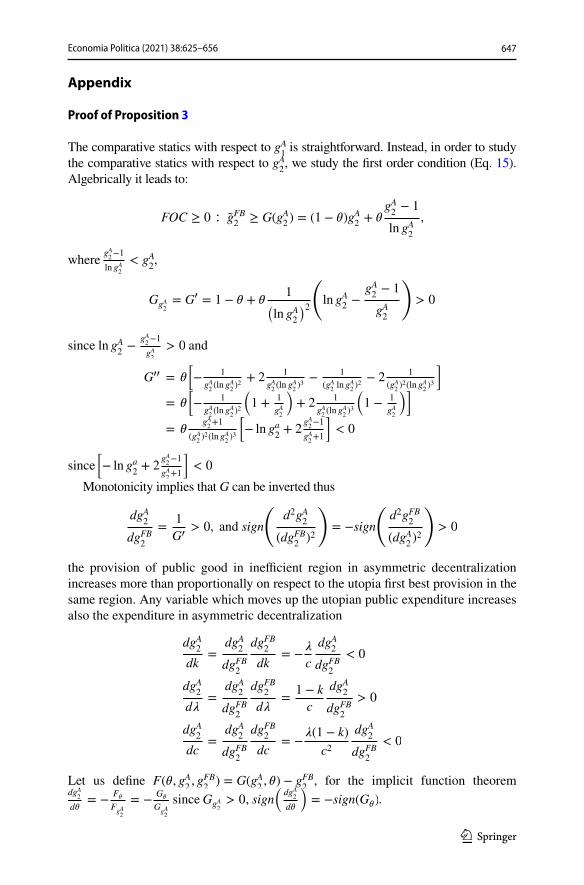
Proposition 3 is proved.The above analysis can be showed in the following graph
gA2
gFB2
gFB2 = λ
c
gFB2 = 1
θ = 0
θ = 1
gA2
gFB2 = λ(1−k)
c
The figure shows that for 1 ≤ gFB2
≤�
c , a unique solution always exists with
gA2≥ gFB
2 . All the variables which increase the utopia point gFB
2 increase also the solu-
tion of Nash Bargaining gA2 . Seemingly, when � increases, the RHS decreases (dashed
lines) rotating clockwise, thus gA2 increases.
Proof of Proposition 5
Region 2 prefers full decentralization to asymmetric decentralization if the following condition is true
where, the left and right hand sides are defined in Eqs. (11) and (7), respectively, considered in their equilibrium outcomes. Thus,
G𝜃 = −gA2+
gA2− 1
ln gA2
< 0, sincegA2− 1
gA2
< ln gA2
y − cgA2+ �(1 − k) ln gA
2+ �k ln
�(1 − k)
c1y − c2
�(1 − k)
c2+ �(1 − k) ln
�(1 − k)
c2+ �k ln
�(1 − k)
c1
Economia Politica (2021) 38:625–656648
1 3
then
We can set z ≡ gA2
gFB2
> 1 . Then,
which is true when z > z , where z means sufficiently high.
z
z − 1ln z + ln c2 − ln c
ln c2 − ln c
zz
We do not know the explicit equation of z . However, we know that region 2 does prefer asymmetric decentralization to full decentralization when z < z , which proves the Proposition given that
Since gA2> gFB
2 , then 1
gA2
dgA2
d𝜃<
1
gFB2
dgA2
d𝜃 . Now, let us consider the value of � , which we
denote with � = � , such that z = z , which is the point in the graph where ln z + ln c2 − ln c = z − 1 , i.e. the point where region 2 is indifferent between full and asymmetric decentralization. Now, any 𝜃 > 𝜃 reduces the threshold to, say, z < z . This, in turn, makes the condition ln z + ln c2 − ln c < z − 1 more likely to be satisfied. Furthermore, note that the threshold needed in order to make full decen-tralization better off for jurisdiction 2 increases in c2 . In order to see that, consider that
(
gA2− gFB
2ln gA
2
)
> gFB2
− gFB2
ln gFB2
− gFB2
lnc
c2
gA2− gFB
2
gFB2
> ln gA2− ln gFB
2− ln
c
c2
ln z + ln c2 − ln c < z − 1,
d
d𝜃(ln z + ln c2 − ln c) =
1
gA2
dgA2
d𝜃> 0 and
d
d𝜃(z − 1) =
1
gFB2
dgA2
d𝜃> 0
Economia Politica (2021) 38:625–656 649
1 3
which proves the Proposition.
Proof of Proposition 6
We compare full centralization (Eq. 5) with asymmetric decentralization for region 1 (Eq. 9), as follows:
Recalling that � ≥ c , the left hand side is weakly positive, as well as the right hand side. Furthermore, when k = 0 the above inequality becomes
that is always true for 𝜆>c . Thus, when k = 0 the efficient region prefers asymmetric decentralization because c1 ≤ c . Instead, as k increases the left hand side remains constant. For k = 1∕2 the right hand side becomes
Thus, it is more likely to prefer asymmetric decentralization either the higher the efficiency ratio ( c
c1) is or the higher the provision of public good in the inefficient
region gA2 is.
Proposition is proved.
Proof of Propositions 8 and 7
We compare asymmetric decentralization for region 2 (Eq. 11) with full centraliza-tion (Eq. 5), as follows:
d
dc2(ln z + ln c2 − ln c) =
1
c2> 0, while
d
dc2(z − 1) = 0,
y − 𝜆 + 𝜆 ln𝜆
c<y − c1
𝜆(1 − k)
c1+ 𝜆(1 − k) ln
𝜆(1 − k)
c1+ 𝜆k ln gA
2,
ln𝜆
c<k + (1 − k) ln
𝜆
c1+ (1 − k) ln(1 − k) + k ln gA
2.
ln𝜆
c< ln
𝜆
c1
1
2
(
1 + ln�
c1+ ln gA
2
)
−1
2ln 2
Economia Politica (2021) 38:625–656650
1 3
Recall the definition z ≡ gA2
gFB2
> 1
When the right hand side (RHS) is greater than the left hand side (LHS), the ineffi-cient region 2 prefers full centralization to asymmetric decentralization.
From the proof of Proposition 3, gA2 increases more than proportionally com-
pared to gFB2
, then dz
dgFB2
> 0 . Since dRHS
dz=
z−1
z> 0 always increases in z,
dRHS
d𝜃=
dRHS
dz
dz
dgA2
dgA2
d𝜃> 0 . Moreover dRHS
dc=
dRHS
dz
dz
dgFB2
dgFB2
dc< 0 . Thus the right hand
side increases with � and decreases with c.Inspecting LHS it is easy to demonstrate that it increases with c and decreases
with c1.Thus, it is more likely that the inefficient region would not use its veto against
asymmetric decentralization if the efficiency of region 1 is sufficiently higher than that of the central government, i.e. if the efficiency ratio c
c1 is high enough.
Moreover, region 1 does not use its veto power when the bargaining leverage of region 1, � , is low. In both cases it is more likely that LHS > RHS . The Proposi-tions 7 and 8 are proved.
Proof of Propositions 9
From Eq. 16, the maximum transfer that the rich region can pay depends on three elements:
• �(k + ln(1 − k)) ≤ 0 is the cost of having a partial and not a full internalization of spillover; note that such element is decreasing in k, i.e. the absolute value of that cost increases with the spillover (k).
• k𝜆 ln z(𝜃) = k𝜆 lngA2
gFB2
≥ 0 is the benefit that the rich region receives by bargaining with the poorer region a level of local public goods greater than the poorer
y − cgA2+ 𝜆
[
(1 − k) ln gA2+ k ln
𝜆(1 − k)
c1
]
< y − 𝜆 + 𝜆 ln𝜆
c
− cgA2+ cgFB
2ln gA
2+ 𝜆k ln gFB
2+ 𝜆k ln
c
c1< −𝜆 − 𝜆 ln(1 − k) + 𝜆 ln gFB
2
− cgA2+ cgFB
2(ln gA
2− ln gFB
2) + 𝜆k ln
c
c1< −𝜆 − 𝜆 ln(1 − k).
−gA2
gFB2
+ lngA2
gFB2
<
−𝜆 − 𝜆 ln(1 − k) − 𝜆k lnc
c1
cgFB2
.
(18)− z + ln z < −
(
1
1 − k+
ln(1 − k)
1 − k+
k
1 − kln
c
c1
)
k
1 − k
(
1 + lnc
c1
)
+ln(1 − k)
1 − k< z − 1 − ln z
Economia Politica (2021) 38:625–656 651
1 3
region optimal level. It increases with � , as we demonstrate in Proposition 3. The effect of k is ambiguous.
• Finally, recalling that c = c1+c2
2 , � ln c
c1−k1
ck2
≥ 0 when 0 ≤ k ≤ 1∕2 is the efficiency gain that the rich region obtains when it pays the local public good at its lower costs, instead of cross-subsidizing the public good of the poorer region. Such value is equal to zero if there is no cost difference between regions. It increases when the cost difference among regions increases since it is the ratio between the arithmetic mean c and the weighed geometric one, where the weight of the lower values is higher ( 0 ≤ k ≤ 1∕2 ). It decreases in k.
Thus, the effect of k on Fmax is ambiguous. in any case, when k = 0 Fmax > FC . Moreover,
thus FMax is decreasing in c1 , while
After rearranging
Proposition 9 is proved.
Proof of Propositions 10
From Eq. 17
• 𝜆(1 − k)[(z − 1) − ln z] > 0 is increasing z . Since z is increasing in the bargaining power, � , Fmin is increasing in the bargaining power of rich region.
• −�[k + ln(1 − k)] ≥ 0 is the cost of not internalizing spillover.• � ln
c1−k2
ck1
c depends on the difference between regions. Note that without spillover
( k = 0 ) it is positive, while for high spillover ( k = 1∕2 ) it is negative.
d
dc1
c1 + c2
2c1−k1
ck2
=1
2ck2
d
dc1
[
(c1 + c2)ck−11
]
d
dc1
c1 + c2
2c1−k1
ck2
=1
2ck2
[
ck−11
+ (k − 1)(c1 + c2)ck−21
]
d
dc1
c1 + c2
2c1−k1
ck2
=1
2
(
c1
c2
)k1
c1
c1 + (k − 1)c1 + (k − 1)c2
c1=
1
2
(
c1
c2
)k1
c1
k(c1 + c2) − c2
c1
d
dc1
c1 + c2
2c1−k1
ck2
=1
2
(
c1
c2
)k1
c1
2kc − c2
c1< 0 since 0 ≤ k ≤ 1∕2 and c2 ≥ c ≥ c1
d
dc2
c1 + c2
2c1−k1
ck2
=1
2c1−k1
d
dc2
[
(c1 + c2)c−k2
]
.
d
dc2
c1 + c2
2c1−k1
ck2
=1
2c1c2
(
c1
c2
)k[
c2 − k(c1 + c2)]
> 0.
Economia Politica (2021) 38:625–656652
1 3
Only with a high difference in regional costs Fmin could become lower then FC . Without cost differences, the poorer region will always request a higher transfers than the one it receives under full centralization in order to accept asymmetric decentralization.
Note that if FA = 0 , the poorer region looses both the internalization of spillover and the financial flow from the rich region (thus it pays more taxes). Therefore, the poorer region uses its veto power against asymmetric decentralization.
The above condition is very similar13 to the one in the proof of Propositions 7 and 8.
Moreover, since c1−k2
ck1
c= 2
c1−k2
ck1
c1+c2
and
which is positive if k is sufficiently high and c1 sufficiently smaller than c2 , otherwise it is negative. Furthermore,
that is negative if k is sufficiently high and c1 sufficiently smaller than c2 , otherwise it is positive.
Proposition 10 is proved.
Proof of Propositions 11.
Fmin < FMax if
d
dc1
c1−k2
ck1
c1 + c2= c1−k
2
d
dc1
ck1
c1 + c2
d
dc1
c1−k2
ck1
c1 + c2= c1−k
2
ck1
(c1 + c2)2
[
2kc − c1
(c1)
]
d
dc2
c1−k2
ck1
c1 + c2= ck
1
d
dc2
c1−k2
c1 + c2
d
dc2
c1−k2
ck1
c1 + c2= ck
1
[
(1 − k)c−k2
c1 + c2−
c1−k2
(c1 + c2)2
]
d
dc2
c1−k2
ck1
c1 + c2=
(
c1
c2
)k1
(c1 + c2)
[
(1 − k) −c2
(c1 + c2)
]
d
dc2
c1−k2
ck1
c1 + c2=
(
c1
c2
)k1
(c1 + c2)2
[
c1 − 2kc]
13 It is the same condition if we impose no transfer ( FC = FA = 0 ) and if we consider institutional spe-cific costs ( c
1≤ c
2= c).
Economia Politica (2021) 38:625–656 653
1 3
then
Since in the parameters’ space z ≥ 1 and k ∈[
0, 1∕2]
,
An agreement is feasible (a necessary condition is Fmax − Fmin > 0 ) only if ln c√
c1c2
is big enough, thus if the difference c2 − c1 is large enough.Moreover,
thus
For a given value of the spillover there exists a maximum value of �∗ such that z∗ =
1
1−k.
Calculating the value in the maximum
that can be positive only if ln c√
c1c2 is big enough.
Moreover,
Thus, the higher the spillover, the higher both �∗ and the difference between c1 and c2 should be in order to have an agreement for asymmetric decentralization.
Besley, T., & Coate, S. (2003). Centralized versus decentralized provision of local public goods: A politi-cal economy approach. Journal of Public Economics, 87(12), 2611–2637.
Biswas, R., & Giuranno, M. G. (2019). Internal migration and public policy. The BE Journal of Eco-nomic Analysis and Policy, 19(4), 1–16.
Buchanan, J. M. (1987). The constitution of economic policy. The American Economic Review, 77(3), 243–250.
Buchanan, J. M., & Tullock, G. (1962). The calculus of consent (Vol. 3). Ann Arbor: University of Michi-gan Press.
Cerniglia, F., Longaretti, R., & Zanardi, A. (2019). Emergence of asymmetric fiscal federalism: Centrifu-gal and centripetal forces. Technical report, Paper presented at the SIEP Conference 2019.
Coakley, J. (2004). The territorial management of ethnic conflict. Abingdon: Routledge.Congleton, R. D. (2006). Handbook of Fiscal Federalism, chapter Asymmetric federalism and the politi-
cal economy of decentralization (pp. 131–153). Cheltenham: Edward Elgar Publishers.Congleton, R. D., Kyriacou, A., & Bacaria, J. (2003). A theory of menu federalism: Decentralization by
political agreement. Constitutional Political Economy, 14(3), 167–190.Conversi, D. (2007). Asymmetry in quasi-federal and unitary states. Ethnopolitics, 6(1), 121–124.Eupolis, Lombardia. (2017). Regionalismo differenziato e risorse finanziarie. Consiglio Regionale della
Lombardia: Technical report.Flynn, M. K. (2004). Between autonomy and federalism Spain. Managing and Settling Ethnic Conflicts
(pp. 139–160). Berlin: Springer.Giuranno, M. G. (2009). Regional income disparity and the size of the public sector. Journal of Public
Economic Theory, 11(5), 697–719.Giuranno, M. G. (2010). Pooling sovereignty under the subsidiary principle. European Journal of Politi-
cal Economy, 26(1), 125–136.Hughes, J. (2001). Managing secession potential in the Russian federation. Regional and Federal Studies,
11(3), 36–68.Jack, W. (2004). The organization of public service provision. Journal of Public Economic Theory, 6(3),
409–425.Keating, M. (2000). The minority nations of Spain and European integration: A new framework for
autonomy? Journal of Spanish Cultural Studies, 1(1), 29–42.Lapidus, G. W. (1999). Asymmetrical federalism and state breakdown in Russia. Post-Soviet Affairs,
15(1), 74–82.Libman, A. (2010). Constitutions, regulations, and taxes: Contradictions of different aspects of decen-
tralization. Journal of Comparative Economics, 38(4), 395–418.Libman, A., & Rochlitz, M. (2019). Federalism in China and Russia. Cheltenham: Edward Elgar
Publishing.MacGarry, J. (2001). Northern Ireland and the divided world: The Northern Ireland conflict and the good
Friday agreement in comparative perspective. Oxford: Oxford University Press.Mangiameli, S., Filippetti, A., Tuzi, F., & Cipolloni, C. (2020). Prima che il Nord somigli al Sud. Rubbet-
tino: Le Regioni tra divario e asimmetria.Martinez-Vazquez, J. (2007). Fiscal fragmentation in decentralized countries. Subsidiarity, solidarity and
asymmetry, chapter asymmetric federalism in Russia: Cure or poison? (pp. 227–266). Cheltenham: Edward Elgar Publishing.
Mintz, J. (2019). Two different conflicts in federal systems: An application to canada. The School of Pub-lic Policy Publications, 12, 14.
Oates, W. E. (1972). Fiscal Federalism. Cheltenham: Edward Elgar Publishing.Oates, W. E. (2005). Toward a second-generation theory of fiscal federalism. International Tax and Pub-
lic Finance, 12(4), 349–373.Ravenda, D., Giuranno, M. G., Valencia-Silva, M. M., Argiles-Bosch, J. M., & García-Blandón, J. (2020).
The effects of mafia infiltration on public procurement performance. European Journal of Political Economy, 64, 101923.
Rizzo, L., & Secomandi, R. (2019). Effetti finanziari delle richieste di autonomia regionale: prime sim-ulazioni. IRPET: Technical report.
Tavares, A. F., & Camöes, P. J. (2007). Local service delivery choices in Portugal: A political transaction costs framework. Local Government Studies, 33(4), 535–553.
Economia Politica (2021) 38:625–656 655
1 3
Tollison, R. D., & Buchanan, J. M. (1972). Theory of public choice: Political applications of economics. Ann Arbor: University of Michigan Press.
Tommasi, M., & Weinschelbaum, F. (2007). Centralization vs. decentralization: A principal-agent analy-sis. Journal of Public Economic Theory, 9(2), 369–389.
Weingast, B. R. (2009). Second generation fiscal federalism: The implications of fiscal incentives. Jour-nal of Urban Economics, 65(3), 279–293.
Williamson, O. E. (1985). The economic institutions of capitalism: Firms, markets, relational contract-ing. New York: Free Press.
Zanardi, A. (2017). Le richieste di federalismo differenziato: una nota sui profili di finanza pubblica. Astrid Rassegna, (11).
Zantman, W. (2002). Constitutional design and regional favoritism. Journal of Public Economic Theory, 4(1), 71–93.
Publisher’s Note Springer Nature remains neutral with regard to jurisdictional claims in published maps and institutional affiliations.