Asymmetric Dynamics in the Correlations Of Global Equity and Bond Returns Lorenzo Cappiello § European Central Bank Robert F. Engle † NYU Stern School of Business and University of California at San Diego Kevin Sheppard ‡ University of California at San Diego Abstract This paper investigates asymmetries in conditional variances, covariances, and correlations in international equity and bond returns. The analysis is carried out through an asymmetric version of the Dynamic Conditional Correlation (DCC) model of Engle (2002), which is particularly well suited to examine correlation dynamics among assets. Particular attention is given to whether changes in the correlation of international asset markets demonstrate evidence of asymmetric response to negative returns. Widespread evidence is found that national equity index return series show strong asymmetries in conditional volatility, yet little evidence is seen that bond index returns exhibit this behavior. However, both bonds and equities exhibit asymmetry in conditional correlation, although in systematically different manners. The paper also examines the strong worldwide linkages in the dynamics of volatility and correlation, finding subtle but important differences between equity and bond second moment dynamics. It is also found that beginning in January 1999 with the introduction of the Euro, there is significant evidence of a structural break in correlation, although not in volatility. The introduction of a fixed exchange rate regime leads to near perfect correlation among bond returns within EMU countries, which is not surprising in consideration of the monetary policy harmonization within the EMU. However, the increase in return correlation is not restricted to EMU countries and equity return correlation both within and outside the EMU also increases after January 1999. JEL Codes: F3, G1, C5 Keywords: International Finance, Correlation, Variance Targeting, Multivariate GARCH, International Stock and Bond correlation §Email. [email protected]†Email: [email protected]‡ Email: [email protected]. Software used in the estimation of this paper can be found at http://weber.ucsd.edu/~ksheppar in the research section. Kevin Sheppard would like to acknowledge financial support from the European Central Bank. While all efforts have been made to ensure that there are no errors in the paper, remaining errors are the sole responsibility of the authors.
Transcript
Asymmetric Dynamics in the Correlations Of
Global Equity and Bond Returns
Lorenzo Cappiello §
European Central Bank
Robert F. Engle†
NYU Stern School of Business and
University of California at San Diego
Kevin Sheppard‡ University of California at San Diego
Abstract This paper investigates asymmetries in conditional variances, covariances, and correlations in international equity and bond returns. The analysis is carried out through an asymmetric version of the Dynamic Conditional Correlation (DCC) model of Engle (2002), which is particularly well suited to examine correlation dynamics among assets. Particular attention is given to whether changes in the correlation of international asset markets demonstrate evidence of asymmetric response to negative returns. Widespread evidence is found that national equity index return series show strong asymmetries in conditional volatility, yet little evidence is seen that bond index returns exhibit this behavior. However, both bonds and equities exhibit asymmetry in conditional correlation, although in systematically different manners. The paper also examines the strong worldwide linkages in the dynamics of volatility and correlation, finding subtle but important differences between equity and bond second moment dynamics. It is also found that beginning in January 1999 with the introduction of the Euro, there is significant evidence of a structural break in correlation, although not in volatility. The introduction of a fixed exchange rate regime leads to near perfect correlation among bond returns within EMU countries, which is not surprising in consideration of the monetary policy harmonization within the EMU. However, the increase in return correlation is not restricted to EMU countries and equity return correlation both within and outside the EMU also increases after January 1999. JEL Codes: F3, G1, C5 Keywords: International Finance, Correlation, Variance Targeting, Multivariate GARCH,
International Stock and Bond correlation §Email. [email protected] †Email: [email protected] ‡ Email: [email protected]. Software used in the estimation of this paper can be found at http://weber.ucsd.edu/~ksheppar in the research section. Kevin Sheppard would like to acknowledge financial support from the European Central Bank. While all efforts have been made to ensure that there are no errors in the paper, remaining errors are the sole responsibility of the authors.
-1-
I. Introduction
Typically, portfolio diversification is achieved using two main strategies: investing in different
classes of assets thought to have little or negative correlation or investing in similar classes of
assets in multiple markets through international diversification. While these two strategies have
both solid theoretical justification and strong empirical evidence exists as to the benefits,
investors must be aware that correlation is dynamic and varies over time, changing the amount of
portfolio diversification within a given asset allocation. In particular, a number of studies
document that correlation between equity returns increases during bear markets and decreases
when stock exchanges rally (see, among others, Erb, Harvey and Viskanta, (1994), De Santis and
Gerard, (1998), Ang and Bekaert, (2001), Das and Uppal, (2001), and Longin and Solnik,
(2001)).
Over the past 20 years, a tremendous literature has developed where the dynamics of the
covariance of assets has been explored, although the primarily focus has been on univariate
volatilities and not correlations (or covariances). Among other regularities, (conditional)
estimates of the second moments of equities often exhibit the so-called “asymmetric volatility”
phenomenon, where volatility increases more after a negative shock than after a positive shock of
the same magnitude; in fact, evidence has been proffered that volatility may fail to increase or
even fall subsequent to a positive shock for certain assets.1 Asymmetric effects have also been
recently found in conditional correlations, although the economic reasoning behind these effects
has not been widely researched.2
The need to take into account the asymmetric effects on conditional second moments has
an appealing economic justification. Assume, for instance, that a negative return shock generates
more volatility than a positive return innovation of the same magnitude. When, as commonly
done, a traditional symmetric Generalized Autoregressive Conditionally Heteroskedasticity
(GARCH) process is used to model second moments, the estimated conditional volatility which
occurs after a price drop will be too small; similarly, the estimated conditional volatility which
follows a price increase will be too large. Consequences such as asset mispricing and poor in-
and out-of-sample forecasts will be, therefore, unavoidable. Accurate estimates of the variance
and correla tion structure of returns on equities as well as other classes of assets are crucial for
portfolio selection, risk management, and pricing of primary and derivative securities.
1 Two explanations have been put forth for this phenomenon: the leverage effect hypothesis, due to Black (1976) and Christie (1982), and the volatility feedback effect proposed by Campbell and Hentschell (1992) and extended by Wu (2000). 2 See, for instance, Kroner and Ng (1999), Bekaert and Wu (2001), and Errunza and Hung (1999).
-2-
Surprisingly, while there has been a proliferation of conditional econometric models able
to capture asymmetry in volatility (see Hentscell (1995) for a synthesis), conditional econometric
specifications able to explicitly model asymmetry in covariances and, above all, correlations are
far less common. However, as argued by Kroner and Ng (1998), if the expected return on one
asset changes due to the occurrence of an asymmetric volatility effect, the correlation (and thus
the covariance) between returns on that asset and returns on other assets which have not had a
change in their expected returns should also change. Although there exist studies which account
for asymmetric effects in conditional covariances, (see, for instance, Braun, Nelson, and Sunier
(1995), Koutmos and Booth (1995), Koutmos (1996), Booth, Martikainen, and Tse (1997),
Scruggs (1998), and Christiansen (2000)), the econometric methodology employed address the
phenomenon through a simplified and not necessarily satisfactorily approach. Apart from the
research of Braun et al.3, time-varying covariances are parameterized in the spirit of Bollerslev
(1990) where the covariance is proportional to the product of the corresponding conditional
standard deviations 4; the correlation coefficient is the proportionality factor and it is assumed to
be constant over the sample period. Although assuming the correlation coefficient constant
greatly simplifies the computational burden in estimation, not only there are no theoretical
justifications to that assumption and it is also not robust to the empirical evidence.
A second generation of multivariate conditional variance models, where the assumption
of constant correlation coefficients is relaxed and asymmetry is explicitly introduced in variances
as well as covariances, has been introduced by Kroner and Ng. Subsequent applications (see, for
instance, Bekaert and Wu (2000), Brooks and Henry (2000), and Isakov and Pérignon (2000))
build on this model. As with most multivariate GARCH model, though, all these representations
suffer from a shortcoming: they usually have too many coefficients to estimate, and the models
are typically of limited scope or significant parameter restrictions must be imposed.
A second stylized fact which emerges from surveying empirical research is that while the
asymmetric phenomenon in (conditional) variances has been widely explored for individual
stocks, equity portfolios, and/or stock market indices, day-to-day changes in government bond
return volatility has received little attention, instead focusing on the impacts of (macroeconomic)
news announcements on conditional volatility of bonds and T-bills.5 Jones, Lamont and
3 Braun et al., who analyze a portfolio of two assets, model the second moment matrix by splitting it into three pieces: The two conditional variances associated with each security and the conditional beta. Also in this case conditional covariances do not exhibit explicit asymmetric effects. 4 The conditional covariances will show an asymmetric response to negative shocks when asymmetric univariate GARCH models are used for the volatilities in the Constant Correlation Coefficient (CCC) model of Bollerslev. However, despite the asymmetric covariances, correlations are constant. 5 In fact, little has been done to explore the correlation structure of bond returns across countries.
-3-
Lumsdaine (1998) detect an increase in the conditional bond market variance on days where
employment and producer price index data are announced. Li and Engle (1998) examine the
effects of macroeconomic announcements on the volatility of US Treasury bond futures.
Scheduled announcements trigger strong asymmetric effects: it is shown that whereas positive
to hold risky assets. But the premia forecast by the traditional GARCH differ from those implied
by an asymmetric GARCH, with a consequence of probable asset mispricing.
While the univariate GARCH literature began by assuming that return volatility was a
linear process of past squared innovations, researchers soon realized that other processes were
both better performing and theoretically justified. Three main changes to the stock GARCH
model have been made to allow the news impact curve (see Engle and Ng (1993)) to take various
shapes depending on the evolution of volatility. The first (in terms of significance of impact) was
to allow the news impact curve to have different responses to positive and negative innovations.
A large number of univariate GARCH models accommodate these effects, including: Exponential
GARCH (EGARCH) introduced by Nelson (1991), Asymmetric Power ARCH (APARCH) of
Ding, Granger, and Engle (1993), GJR-GARCH of Glosten, Jaganathan, and Runkle (1993),
Threshold GARCH (ZARCH) of Zakoian (1994), thereafter extended by Rabemananjara and
-5-
Zakoian (1993),6 just to name a few. The second change to the original news impact curve was to
allow the shocks to enter non-linearly (through a Box-Cox like transformation) into the variance.
Models which allow this effect include Nonlinear GARCH (NGARCH) of Higgins and Bera
(1992) and APARCH. The third major change to the news impact curve has been to allow for a
re-centering of the curve, so that the point of no change in the volatility is not necessarily
centered at zero; AGARCH (Engle (1990)) and NAGARCH (Engle and Ng (1993)) allow for this
type of asymmetry. Hentschell (1995) has proposed a model which encompasses these three
effects and provides an overview of the above mentioned univariate asymmetric GARCH
parameterization. Recent evidence (Hansen and Lunde (2001)) has shown that not only do these
models perform better in-sample, but they also produce superior forecasts.
While asymmetries in conditional volatilities have been thoroughly empirically verified,
the efforts to capture asymmetric effects in multivariate settings, however, have been far rarer.
Presently, there are only two models capable of capturing asymmetric effects in correlation in a
multivariate GARCH model. The first to model asymmetric effects was Kroner and Ng. The
model they proposed allows for asymmetric effects in both the variances and covariance. An
alternative multivariate GARCH parameterization which permits to capture asymmetries in
variances (but not in correlations) is the Dynamic Conditional Correlation (DCC) GARCH model
of Engle (2002). As pointed out in Engle and Sheppard (2001), any univariate GARCH model
which is covariance stationary and assumes normally distributed errors (irrespective of the true
error distribution) can be used to model the variances, as the model is estimated in two steps: the
first in which variances are estimated using a univariate GARCH specification, and the second
where the parameters of the dynamic correlation are considered. Sheppard (2002) has recently
extended the DCC model to allow for asymmetric dynamics in the correlation in addition to the
asymmetric response in variances (which were available in the original DCC model). Moreover,
while the original DCC model assumed that all assets shared the same news impact curve for
correlation, Sheppard’s specification is able to accommodate different news impact curves for
correlations across distinct assets.
Economically, asymmetric volatility can be explained by two models: leverage effect and
time-varying risk premia (volatility feedback). The leverage effect, simply put, states that after a
negative shock, the debt-to-equity ratio of a firm has increased. Thus, the volatility of the whole
firm, which is assumed to remain constant, must be reflected by an increase in volatility in the
6 The first version of Zakoian's threshold GARCH appeared in a working paper (CREST, INSEE) dated 1990. This explains why the extension of the model due to Rabemananjara and Zakoian (1993) has an earlier date than the original model published only in 1994.
-6-
non-leveraged part of the firm (equity). Christie (1982) was one of the first to provide empirical
evidence of the leverage effect, finding a positive correlation between the leverage ratio and the
volatility of the firm. An alternative explanation of the larger increase in volatility after a
negative shock proffered by Campbell and Hentschel (1992) is that after a negative shock and
variance increase, the expected return must become sufficiently high to compensate the investor
for the increased volatility, thus creating more volatility (volatility feedback). These two
explanations for asymmetries in volatility are not exclusive, and Bekaert and Wu (2000) have
combined these two explanations in an empirical model and have shown that the leverage effect
alone does not adequately explain the changes in volatility after a decrease in the asset price.
Both of these explanations for larger volatility subsequent to a negative shock have
primarily focused on the volatility of equities, although the Campbell and Hentschel model is
applicable to bonds as well as stocks, through the CAPM, treating bonds as risky assets (see
Cappiello, 2000). However, as bonds do not have leverage, the leverage effect is implausible.
Further, while there is compelling evidence that bond volatility increases after announcement
about macroeconomics news, it is yet to be seen if the asymmetric effect is present in the day to
day volatility dynamics of government bonds.
In addition to possible explanations for asymmetries in bond return volatility, little
theoretical framework is available to explain the recent evidence of asymmetric response to joint
bad news in correlations (joint bad news refers to both returns being negative). While certain
models can capture these effects, there has been little done to explain their presence. One
possible explanation rests on time-varying risk premia. More precisely, if, due to negative
shocks, the variances of two securities increase, in a CAPM-type world, investors will require
higher returns to compensate the larger risk they face. As a consequence, prices of both assets
will decrease and asset correlation will go up, as it usually happens in down markets. Correlation
may therefore be higher after a negative than a positive innovation of the same magnitude,
indicating its sensitivity to the sign of past shocks. However, this idea has not yet been
formalized in a multivariate model. Another plausible explanation is that dependence in returns
is higher for large negative returns, and possibly nonlinear. In this case the increased correlation
observed is simply a linear approximation to the nonlinear dependence. Recently, Patton (2002)
has shown that correlation provides a good approximation to the dependence structure of
portfolios of large and small cap stocks. However, it is yet to be seen how widespread this
phenomenon is.
-7-
III. Econometric Methodology
While there has been wide empirical evidence of asymmetries in volatilities, recent studies
(Kroner and Ng (1998), Baekert and Wu (2000), and Cappiello (2000)) have also provided
limited evidence for asymmetries in covariance above those which would be present under an
assumption of asymmetric volatilities but with constant correlation. In order to investigate the
properties of international equity and bond returns, we have chosen to use a recently introduced
generalization of the DCC (Engle (2002)) model. The general form of the model employed in
this paper was developed in Sheppard (2002), and includes two modifications to the original DCC
model: asset specific correlation news impact curves and asymmetric dynamics in correlation.
All DCC class models (including the Constant Correlation Coefficient-GARCH (CCC-
GARCH) of Bollerslev (1990)) assume that a 1×k vector of asset returns tr are conditionally
normal with mean zero and covariance matrix tH
( )ttt HNr ,0~| 1−ℑ , (1)
and use the fact that Ht can be decomposed as follows:
tttt DRDH = , (2)
where tD is the kk × diagonal matrix of time-varying standard deviations from univariate
GARCH models with t,ih on the ith diagonal and tR is the (possibly) time-varying correlation
matrix. 7 The DCC model was designed to allow for two-stage estimation of the conditional
covariance matrix tH : in the first stage univariate volatility models are fitted for each of the
assets and estimates of t,ih are obtained; in the second stage asset returns, transformed by their
estimated standard deviations resulting from the first stage, are used to estimate the parameters of
the conditional correlation. The original DCC estimator had the dynamics of correlation evolving
as a scalar process with a single news impact parameters and a single smoothing parameter.
However, for higher dimensional models and certain assets, this proved to be inadequate, and the
Asymmetric Generalized DCC estimator was developed to capture the heterogeneity present in
the data. The model used in this paper is a restricted version of the AG-DCC model.
As asymmetries in volatilities are a widely accepted empirical fact, the univariate
volatility models will be selected using the Schwartz Information Criterion (BIC) from a class of
7 The assumption of conditional normality is not crucial and in the absence of conditional normality, these results have a standard QMLE interpretation.
-8-
models capable of capturing the common properties of equity return variance.8 The following
models were included in the specification search (all with one lag of the innovation and one lag of
volatility)
• GARCH (Bollerslev (1996))
• AVGARCH (Taylor (1986))
• NARCH (Higgins and Bera (1992))
• EGARCH (Nelson (1991))
• ZARCH (Zakonian (1994))
• GJR-GARCH (Glosten, Jaganathan, and Runkle (1993))
• APARCH (Ding, Engle and Granger (1993))
• AGARCH (Engle (1990))
• NAGARCH (Engle and Ng (1993))
The simplest of the models are GARCH, AVGARCH (GARCH on standard deviations instead of
variances) and NARCH, followed by GJR-GARCH, ZARCH, and EGARCH (which all allow for
threshold effects but use different powers of the variance in the evolution equation), and
APARCH (which encompass both threshold effects and an estimated power for the evolution of
variance). AGARCH and NAGARCH both differ in that asymmetries in the news impact curve
come through re-centering of the curve, instead of a slope change which depends on the sign of
past innovations. Appendix C contains exact specification employed for these models.
Once the univariate volatility models are estimated, the standardized residuals,
ititit hr=ε , are used to estimate the dynamics of the correlation. The evolution of the
correlation in the standard DCC model (Engle (2002)) is given by
111)1( −−− +′+−−= tttt bQaQbaQ εε (3)
1*1* −−= tttt QQQR (4)
where [ ]ttEQ εε ′= and where a and b are scalars. However, as this model does not allow for
asset specific news impact parameters nor asymmetries, the evolution equation has been modified
8 While there are many information criteria available, in addition to likelihood ratio testing using nested models, we felt that the use of the BIC was appropriate as it will lead to asymptotically correct model specification selection.
-9-
where A , B , and G are diagonal parameter matrixes, [ ] ttt In ε<ε= o0 (with o indicating the
Hadamard product), [ ]ttnnEN ′= . For Q and N , expectations are infeasible and are replaced
with sample analogues, ∑ =− ε′ε
T
t ttT1
1 and ∑ =− ′T
t tt nnT1
1 , respectively. [ ] [ ]t,ii*
t,ii*t qqQ == is a
diagonal matrix with the square root of the ith diagonal element of Qt on its ith diagonal position.
In other words, *tQ is a matrix which guarantees 1*1* −−= tttt QQQR is a correlation matrix with
ones on the diagonal and every other element less than one in absolute value, as long as tQ is
positive definite.9 The typical element of tR will be of the form t,jjt,iit,ijt,ij qqq=ρ . The
immediate implication is that tR will necessarily be a correlation matrix by the Cauchy-Schwartz
inequality (see Engle and Sheppard (2001) for a formal proof). Four special cases of this model
(equations 3 and 4) exist, the CCC multivariate GARCH [ ]( )0=G,A , the DCC multivariate
GARCH [ ] [ ] [ ]( ,aaA,G ij === 0 [ ] [ ])bbB ij == , the asymmetric DCC (ADCC) multivariate
GARCH [ ] [ ]( ,aaA ij == [ ] [ ],bbB ij == [ ] [ ])ggG ij == , and the generalized diagonal
DCC (GDDCC) multivariate GARCH model [ ]( )0=G . It is also simple to extend the model to
allow for structural breaks in either mean or dynamics. For instance, let d be 0 or 1, depending
on whether Tt <> τ . Then to examine whether a structural break has occurred, the model can
be modified to
( )GnnGBQBAA
GNGdGNGBQBdBQBAQAdAQAQdQQ
ttttt
t
11111
~~~
−−−−− ′′+′+′′+′+′−′+′−′+′−−=
εε (6)
where [ ] τεε <′= tEQ tt , , and [ ] τεε ≥′−= tEQQ tt ,~
, with N and N~
analogously
defined, which is equivalent to the following parameterization (where
[ ] [ ] ττ ≥=<= teeEQteeEQ tttt ,',,' 21 ) when mean reversion is enforced
( ) ( ).' 11111
22221111
GnnGBQBAAGNGBQBAQAQGNGBQBAQAQQ
ttttt
t
−−−−− ′′+′+′+′−′−′−+′−′−′−=
εε (7)
As the model in equation 6 nests the standard model (equation 3), it is straight forward to test for
breaks in the mean of the process. The test can be conducted using standard likelihood ratio tests
with k(k-1)/2 d.f. Breaks in dynamics as well as breaks in both dynamics and mean can be tested
for analogously (although with different d.f.).
9 tQ will be positive definite with probability one if ( )GQGBQBAQAQ ′−′−′− is positive definite.
-10-
Kroner and Ng (1998) introduced a notion for multivariate GARCH models analogous to
a news impact curve for univariate models, a news impact surface. For the model considered in
this paper, the news impact surface for correlation will be asymmetric, having (potentially)
greater response to joint bad news (both returns less than zero) than to joint good news. The
news impact surface for correlation is given by
( ) ( )( ) otherwiseaacf
forggaacf
jijiij
jijijiij
,~,
0,,~,
21
2121
εεεε
εεεεεε
+≈
<++≈, (8)
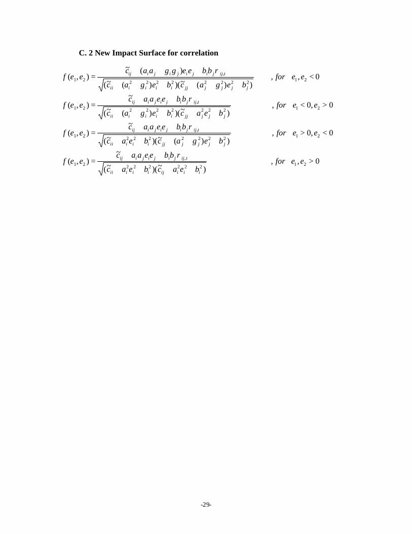
where 21 ,i,i =ε are the standardized residuals.10 The news impact surface for covariance will
simply be the news impact surface for correlations multiplied by the appropriate portion of the
news impact curve for the univariate models, which can be very different should the models for
the univariate volatilities be drastically different, producing asymmetries in covariance in all four
directions from the origin.
IV. Data
The data employed for this paper consists of FTSE All-World Indices for 21 countries and
DataStream constructed 5 year average maturity bond indices for 13.11 The FTSE All-World
Index Series are a measure of a well diversified investment in a particular country using a value
weighted average. These indices are constructed using 90% of the equity value in a country
consisting of large- and medium-caps, and represent the total return on equities as the indices are
dividend adjusted. The DataStream Benchmark bond indices consist of the most liquid
government bonds and follow the European Federation of Financial Analysts (EFFAS)
methodology. These bond indices are available daily and are chain linked allowing the addition
and removal of bonds without affecting the value of the index. All data were taken from
DataStream and converted to US dollar denominated returns (appendix A contains a complete list
of the equity and bond indices included in this study). The selected 21 countries contain most of
the present day EU, the major markets of the Americas, both developed and developing, and the
major markets of Australasia.12 One of the primary concerns when working with international
data, specifically asset correlation, is that non-synchronous trading issues can arise which will
10 This formula is approximate, due to the non-linear transformation needed. The exact news impact surface is given in appendix C.2. 11 The actual series were the DataStream Benchmark Bond Indices with 5 years average maturity (code BMXX05Y where XX is the country code). 12 The 13 included bond markets are a proper subset of the 21 included equity markets and include all of the major world government bond markets.
-11-
lead to a downward bias in the estimated correlation. Martens and Poon (2001) have shown that
using non-synchronous data results in a significant downward bias in correlation, as compared to
pseudo-closes.13 However, with the global scope for this paper, there is never a time when all 21
markets are open. Thus, weekly returns were used instead of daily to alleviate the problem of
asynchronous closes.
The data contain 15 years of weekly price observations, for a total of 790 observations from
January 2, 1987 until February 15, 2001. All weekly returns were calculated through log
differences using Friday to Friday closing prices. To begin analyzing this data set, it is
informative to examine the unconditional correlation among the various stock and bond series.14
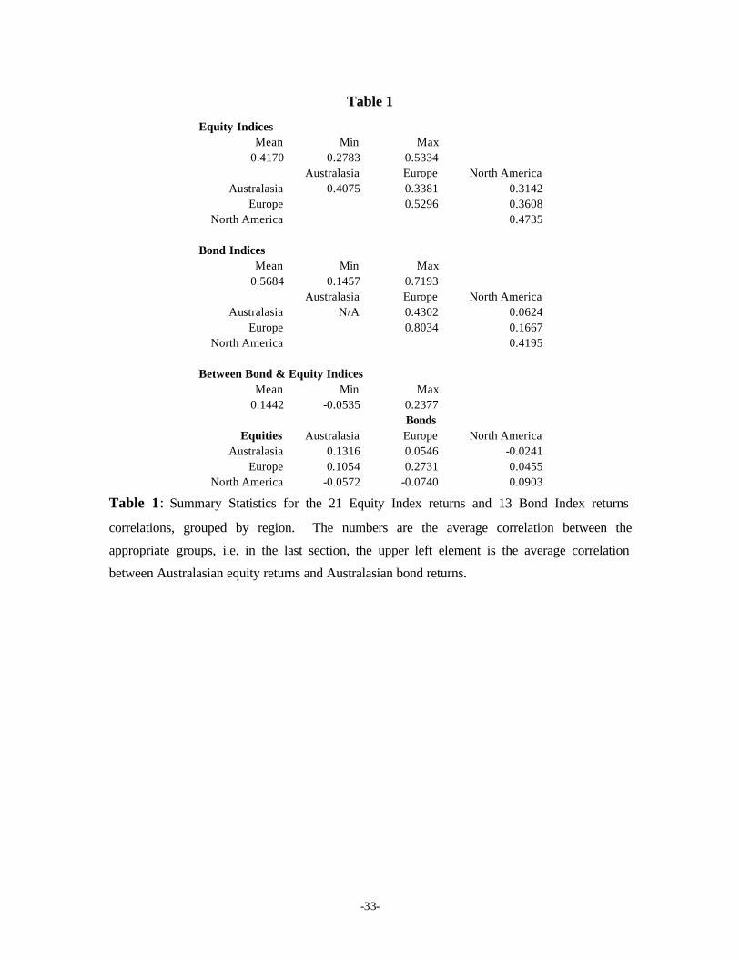
Table 1 summarizes information about the distribution of correlations between the equity series,
the bond series, and correlations between the equity series and the bond indices, while table 2 (a,
b, and c) contains the unconditional correlation for each of the 34 assets. While the distribution
of the average correlation for groups of assets is difficult to calculate, we were able to conduct
significance test using the bootstrap distributions of these statistics.15 The bootstrap distribution
was tabulated using the stationary bootstrap (Politis and Romano (1994)) with an average
window length of 13 weeks (based on initial estimates of the persistence of correlation across all
assets). When statistical significance is indicated, it means that the empirical quantile of the
bootstrap distribution is less than (or greater than, depending on the test) the statistic.
Overall the assets are reasonably correlated with a median correlation of 0.2986. However,
there is a wide range of correlation among the assets, ranging from an average of 0.0808 for US
bond index returns to 0.4498 for Dutch equities. Overall, the average correlation for the equity
series (.3401) is similar to the overall average correlation for the bond indices (.3270). However,
while on average they appear the same, asset returns are highly correlated with their own type and
less correlated with the other type, or in other word, the equity-equity and bond-bond correlations
are far higher than equity-bond correlations. In fact, median bond-bond return correlation was
0.7276, median equity-equity correlation was 0.4435, and median equity-bond correlation was
only 0.1849, with all three means being statistically different from the other two at the 1% level.
13 Pseudo-closes are simply constructed by sampling all prices at the same time GMT. 14 The unconditional correlation could be considered as a naïve estimate in the presence of heteroskedasticity, and will underestimate the average conditional correlation between the innovations. 15 While the correlations should be asymptotically multivariate normally distributed, the computation of the asymptotic covariance matrix would be made more difficult as the models are dynamically misspecified requiring an adjustment to the White robust standard errors to account for autocorrelation in the scores of the correlation estimator.
-12-
Among the equity index return series, the mean correlation was 0.4137. The equity market
with the highest average correlation was The Netherlands with 0.5355 while both Japan and
Mexico exhibited the lowest average correlations at 0.2604 and 0.2826 respectively. The intra-
stock index return correlations demonstrated a strong increase in correlation when considered at
the regional level. In this sample, there exist three clear geographic groups for the data:
Australasia, Europe and North America.16 Within the Australasian subgroup the average
correlation was 0.4032, while the average correlation between equity index returns in the
Australasian group and the European group was 0.3858, and 0.3052 with North American
markets. Average correlation among the European markets was 0.5289, while European and
North American markets had an average correlation of 0.3386. Finally, the average correlation
within the North American equity markets was 0.4590. 17 The correlations within both the
European and American were statistically significantly higher than were the correlations between
these two groups and the others. In addition, the correlation within the Australasian group was
statistically higher than the correlation between the North American group and the Australasian
group.
Turning attention to the correlation between the bond indices, there also appears to be distinct
groups for the unconditional correlation of bond returns: Europe, Japan, and North America.
Within European bond markets, average correlation between returns was 0.7894, while average
correlation between European markets and Japan was 0.4134 and average correlation between
European bond index returns and North American bond returns was 0.1508. Correlation among
North American bond returns (Canada and the United States) 0.4523 while average correlation
between American bond returns and Japanese bond returns was 0.0225.18 As was the case with
the mean equity indices, the mean intra-region correlations were statistically greater than the
mean inter-region correlations.
Finally, the average correlation (as per expectations) between the equity index returns and the
bond index returns was significantly lower than the intra-stock or intra-bond index return
correlation. The mean inter-stock-bond correlation was 0.1500, significantly lower than the
average intra-stock correlation of 0.4137 or the average intra-bond correlation of 0.5535. Further,
the inter stock-bond correlations were the only subset of the correlation to have any statistically
significant negative values. In addition, every equity return series had at least one bond index for
16 Group membership is listed in Appendix C. 17 The correlation between the US and Canadian equity index returns was 0.6924. The correlation between Canadian and US markets with Mexican equities was much lower, 0.3040 and 0.3806, respectively.
-13-
which it was either insignificantly correlated with or significantly negatively correlated with.
This is clearly an important point in that one would expect efficient portfolios to generally hold
both equity and bonds as they provide insurance (although in a limited fashion) against the other.
This further confirms that the negative correlation between bonds and equities ubiquitous across
nations.
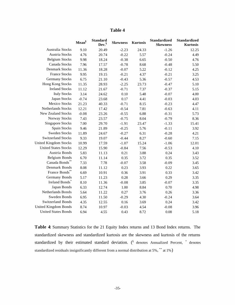
Turning our attention from unconditional second moments to univariate properties of the
data, we find that the data possess the standard properties of financial returns. Namely, both bond
and stock returns are leptokurtotic, with stock returns having negative skew and bonds, on
average, positive skew. Table 4 contains a summary of the univariate statistics for the system.19
All markets, save New Zealand and Japan produced an average positive return during the sample,
with Mexico producing by far the highest average return, annualized at a rate of 21.2%. All save
two of the equity index return series were left skewed, with an average skewness of -.68. The
raw equity index returns also exhibited extreme excess kurtosis, with an averaging 6.45. It is well
know that while heteroskedastic return series can exhibit skewness and fat-tails, returns
standardized by their estimated conditional standard deviation can be normal (or close to normal).
To investigate the properties of the innovations, we standardized the residuals by the preferred
GARCH model (see section 3). While the residuals standardized by their estimated standard
deviation are both less skewed (average -.48) and less fat-tailed (averaging 3.05 excess kurtosis),
the standardized residuals are highly non-normal. In fact, all 21 equity index return series, even
when standardized by an estimated conditional standard deviation, reject normality using a
Jarque-Bera test at the 1% level.
Unlike the volatile equity indices, the bond index returns were more homogeneous,
having annualized returns ranging from 4.35 to 8.74 with a mean of 6.68 and having uniformly
lower standard deviations than the least volatile equity index. Nine of the 13 bond index return
series were positively skewed, having an average skewness of 0.21, and were leptokurtotic with
an average excess kurtosis of 1.64. The bond index returns standardized by their estimated
conditional standard deviations were, again, slightly less skewed, with an average skewness of
0.17 and less fat-tailed, averaging an excess kurtosis of 0.74. As was the case with equity returns,
bond index returns typically reject the null of normality. Only the Irish bond index returns do not
reject normality at the 5% level using a Jarque-Bera test, with Canadian and French bond index
returns also failing to reject the null at the 1% level.
18 Only the average correlation between North American bond returns and Japanese bond returns was insignificantly different from zero (.0382). 19 Both mean and standard deviation are reported as annualized percent.
-14-
Finally to investigate asymmetries in variances and correlation, we can examine if the
variance of asset returns are higher after a negative shock than after a positive one. We calculate
the [ ]012 <−itit r|rE and test the null that [ ] [ ]00 1
21
2 >=< −− itititit r|rEr|rE . If there were an
asymmetric increase in the level of variance after a negative shock, we would expect that
( ) ( ) 02 0
21
2 02 02
1
2 0 1111>− ∑∑∑∑ = >
−
= >= <
−
= < −−−−
T
t ritT
t rT
t ritT
t r ititititIrIIrI . Nineteen of the equity indices
had variances after a negative shock greater than after a positive shock, and eleven of these
differences were significant at a 10% level, while nine of the bond indices had larger variances
after negative shocks, although only one was significant. Following the same line of analysis, we
can investigate if the average covariance of the standardized residuals ( [ ] t,ijjtittE ρ=εε−1 ) after
joint negative returns is different than after two positive returns by testing
( ) ( ) .IIIIIIIIT
t jtitT
t
T
t jtitT
t jititjititjititjtit0
2 00
1
2 002 00
1
2 00 11111111>εε−εε ∑∑∑∑ = >ε>ε
−
= >ε>ε= <ε<ε
−
= <ε<ε −−−−−−−−
Every of the equities exhibited significant increases to joint bad news in at least one series, with
the United States having the most significant at the 10 level (13), than to joint good news, while
only 6 of the bond series exhibited this behavior. Table 3 contains the estimated conditional
volatility and conditiona l correlation for the equity and bond market returns.
V. Empirical Results
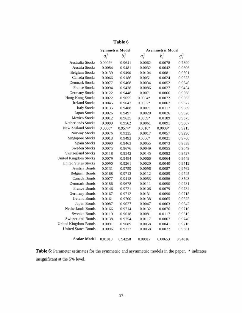
The first stage of the model building consisted of fitting the univariate GARCH models for each
of the 34 data series and selecting the best one using information criteria. Table 5 contains the
specification of the GARCH processes selected by the BIC and the estimated parameters from
these models. Eighteen of the 21 models selected for the equity return series contained a
significant asymmetry term. Of the 18 models with asymmetries, the vast majority (16) preferred
the introduction of the asymmetry via the inclusion of threshold effects, with only two preferring
a re-centering of the news impact curve (both using the AGARCH model). As widespread as the
evidence of asymmetry vola tility was in the equity series, it was equally absent from the bond
index return series. Only 3 of the 13 models selected exhibited asymmetric effects, all of the
threshold variety. This is consistent with the earlier evidence of little conditional difference in
variances after negative shocks for bond returns. Interestingly, though, as explained below, bond
(as well as equity) returns exhibit asymmetry in conditional correlation. Figure 1 contains the
news impact curves for five of the assets. The dramatically different shapes highlight the
flexibility of this modeling approach. For instance, the model selected for Swiss equity returns
-15-
was an EGARCH with a negative parameter on the innovation and a positive parameter on
absolute value of the innovation resulting in a news impact curve which is extremely asymmetric,
indicating a much smaller increase in volatility after a positive shock. Likewise, the news impact
curve for Canadian bond return volatility is near zero for all positive shocks and only increases
for negative ones, while the Swiss bond returns show an asymmetric response to good news with
a larger increase in volatility subsequent to a positive shock.
Four different models were estimated for the dynamics of the correlation. The first, and
simplest model, was a standard scalar DCC (i.e. each of the matrices, A and B, are diagonal with
the same value on each diagonal element and no asymmetric terms are included). Next the full
diagonal version of the model was estimated allowing for no asymmetries in the correlation
dynamics. The two forms of model estimated were an asymmetric DCC model (A, B and G each
consist of a single unique element) and the full diagonal version of this model where asymmetric
terms were introduced allowing for different news impact and smoothing parameters across the
assets. Upon inspection of the fit correlation and the data, it became obvious that a large number
of the series have undergone a significant structural break when the exchange rates were
irrevocably fixed. In order to correct for this obvious deficiency, all of the 4 base models were
modified to allow for a structural break in the mean and for both a structural break in the mean
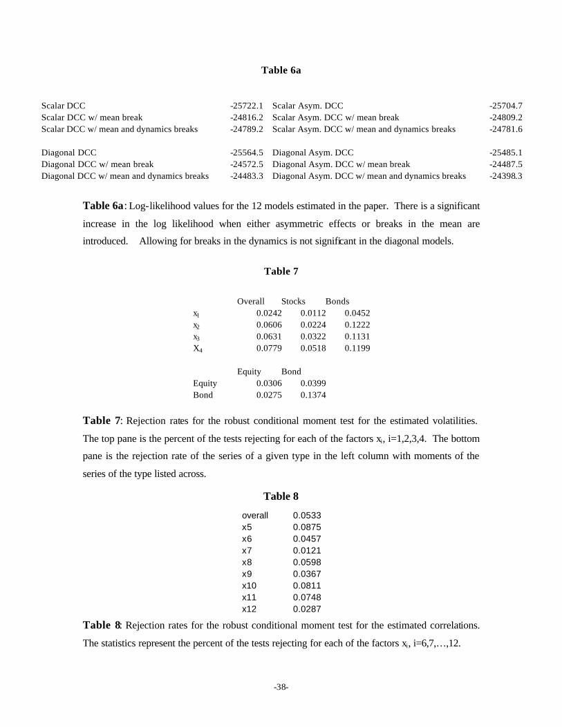
and in the dynamics across the introduction of the Euro. Tables 6 and 6a contains the results of
the estimated models, with the results presented for the parameters of the models where the mean
was allowed to change but not the dynamics. Almost all of parameters in the models estimated
were significant, with exceptions noted in the table. The first observation is that the diagonal
versions of the models significantly outperform the scalar versions of the same model. In
addition, both of the asymmetric DCC models outperform their non-asymmetric DCC
counterparts, with p-values of zero. The shocks to correlation were typically highly persistent,
with a half-life of more than 14 weeks for the simplest symmetric scalar DCC model. For the
diagonal DCC model, two of the assets series exhibited no (or nearly no) innovation, and for
those which did, the half-life of the innovation ranged from 9 to over 63 weeks. In order to
calculate the expected half life of an innovation for the asymmetric model, it is necessary to use
expected value or by assuming symmetry for the distribution. Overall, the asymmetric models
produces slightly less persistence, but were also highly persistent.
-16-
We also found significant evidence of a structural break when the EMU exchange rates
were irrevocably fixed20. We tested for both a structural break in the mean and a structural break
in both the mean and the dynamics. The likelihoods of these 12 models (3 treatments of the
original 4 models) are in Table 6a. We overwhelmingly reject the null of no structural break in
the mean for all models (typical likelihood ratios were approximately 1800 with 561 degrees of
freedom), yet find no compelling evidence for both a break in the mean and the dynamics. In
addition, allowing for a break reduced the persistence of the series to typically 3 to 10 weeks. We
see this as further evidence in support of the break, as series with unconditional shifts are known
to produce longer memory that properly modeled series. The remainder of the paper will present
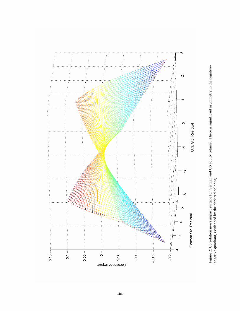
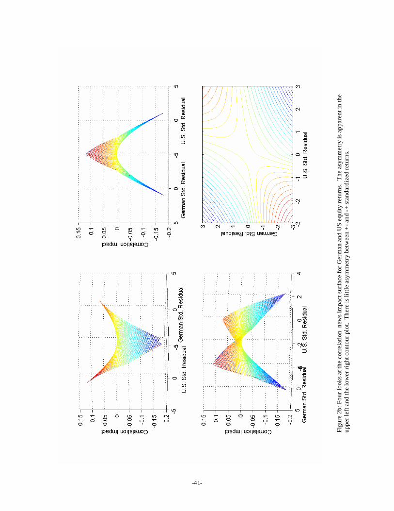
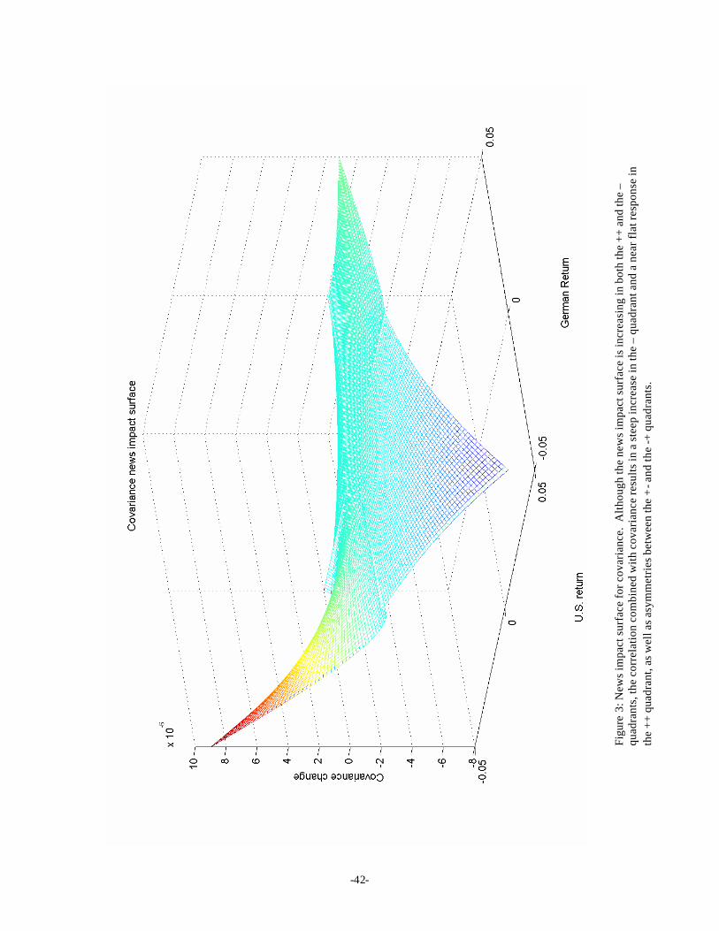
the AG-DCC model with a break in the mean but not in the dynamics. Figures 2 and 3 contain
news impact surfaces for German-US equity correlation and covariance respectively. The
correlation news impact surface is highly asymmetric, showing a larger response to in the --
quadrant news than in the ++ quadrant (i.e. more responsive to joint bad news than to joint good
news of the same magnitude). However, when the correlation and volatilities are simultaneously
considered, the asymmetry becomes even more striking, with a huge increase for joint negative
shocks, little change even for larger positive shocks, and asymmetries in all 4 quadrants.
V.1 Specification Testing
In order to verify if the specification selected adequately explains the dynamics in the
data, we made us of the robust conditional moment tests (Wooldridge (1990, 1991)). The test is
useful in detecting whether a variable (or a function of that variable) is useful in predicting a
generalized residual tiju , (a generalized residual is a constructed residual, such as ititt hru −= 2
or ( ) 12 −= ititt hru , which should have conditional expectation zero). This resulting statistic
tests if a set of moment conditions, 1, −tgx , can predict the generalized residual series. The test
statistic is given by
( ) ( )1
1
21
22
11 11
−
=−
=−
λ
λ= ∑∑
T
tt,gt,j
T
tt,gt,ij uTuTC (9)
20 While it would be ideal to test each series for a break at all points in time, it is infeasible to follow this course as the parameters of the model will not be identified under the null of no break, making standard testing theory incorrect. The choice of allowing the break to occur at the introduction of the Euro was driven by the expected increase in correlation among EMU countries, and possible increases in other countries toward the end of the sample.
-17-
where 1, −tgλ is the residual from a regression of the moment conditions on the scores of the
likelihood. Under mild regularity conditions, C is asymptotically distributed )1(χ . The test is
relatively simple to compute, as it can be conducted using two regressions: the first where the
moments are regressed on the scores of the estimated model, and the second where a vector of
ones is regressed on the product of the generalized residuals and the residuals from the first
regression. The moment conditions can be any function of any variable in the conditioning set.
However, in order to keep the analysis tractable, we focus on a few types of potential
misspecification. The first and simplest is whether the sign of a lagged return can predict future
volatility. In other word, [ ]011 <= −− tit rIx is a binary variable that indicates whether the past
return was negative. Analogously, we can construct variables which measure a positive impact,
or whether the signed magnitude of a past innovation can predict future volatility. In examining
the volatility models, we used 4 different criteria.
[ ][ ]
[ ][ ]0
0
00
12
114
12
113
112
111
>=
<=
>=<=
−−−
−−−
−−
−−
ttt
ttt
tt
tt
rIrx
rIrx
rIxrIx
(10)
In testing the volatility models selected, 34 x 34 x 4 (4624) tests were conducted (34 generalized
residual series, 34 potential series to get the moment conditional from, and 4 different moments to
choose from). The generalized residual was defined as tititi hru ,2,, −= . The overall rejection rate
was extremely close to size at 0.0705 using a size of 5%. However, the rejection rate for bonds
was higher than the rate for equities, with the majority of the bond rejections resulting from
misspecification tests using equity returns as moment indicators indicating that equity return
volatility may spill over to bond markets possibly through a flight to quality. Table 7 contains
more detailed information on the types of rejections and the rejection for bonds and stocks as
groups.21
We also tested the correlation estimates by stacking the T x k x (k-1)/2 generalized
residuals tijtjtitiju ,,,, ρεε −= (the outer product of the standardized residuals minus the
estimated correlation) using the following 8 moment conditions (for each of the 33 x 17 off
diagonal series):
21 We also tested the generalized residuals against only moments created using their own lagged data, and found the rejection rate was significantly under size at 0.0074.
-18-
[ ] [ ][ ] [ ][ ] [ ][ ] [ ]
[ ] [ ][ ] [ ][ ] [ ][ ] [ ]00
00
00
00
00
00
00
00
1111112
1111111
1111110
111119
1118
1117
1116
1115
>ε>εεε=
>ε<εεε=
<ε>εεε=
<ε<εεε=
>ε>ε=
>ε<ε=
<ε>ε=
<ε<ε=
−−−−−
−−−−−
−−−−−
−−−−−
−−−
−−−
−−−
−−−
t,jt,it,jt,it
t,jt,it,jt,it
t,jt,it,jt,it
t,jt,it,jt,it
t,jt,it
t,jt,it
t,jt,it
t,jt,it
IIx
IIx
IIx
IIx
IIx
IIx
IIx
IIx
(11)
This results in a total of 8 x 17 x 33 (4488), one for each of the 8 moment indicators for
each of the above diagonal elements of Rt. Table 8 contains the percentage rejection for these
tests. Overall the rejection rate was near size at 0.0533, and across the 8 moment indicators, the
performance was relatively equal, with no single indicator causing a disproportionately large
number of rejections. Based on the robust conditional moment test, we feel the AG-DCC model
with a break in the mean adequately describes the data.
V.2 Volatility Dynamics and Linkages
While each of the volatility series was assumed to evolve independently of the other series, the
model allows us to examine the volatility linkages across the countries. A simple criterion to
examine these linkages is the correlation between the estimated volatilities of two assets:
( )( )
( ) ( )∑∑
∑
==
=
−−
−−=ρ
T
tjjt
T
tiit
T
tjjtiit
hh
hhhh
hhhh
jtit
1
2
1
2
1 (12)
Overall, the volatilities of the equity markets were reasonably correlated, with an average
correlation of 0.3245, and were similar both pre- and post-introduction of the fixed exchange rate
regime system in Europe. However, there were strong regional effects in the linkages. For
instance, the correlation of the volatility of European equity market returns was 0.5457 over the
entire sample, and was also similar across the introduction of the euro. The American equity
markets’ volatilities were also extremely correlated, averaging 0.6115, while the correlation
between US and Canadian equity volatility was extremely high at 0.7963. Australasian equity
volatility correlation was similar to the over all average at 0.4175, although this was in part due to
extremely low correlation between the volatilities of New Zealand with the rest of this group. As
was the case with equity returns, correlation of equity volatilities are much lower across group
-19-
than within. Also not surprising, the correlation among the volatilities of larger markets was
higher with volatility between France, Germany, and US, and the UK equity markets averaging
0.7062.
Figure 4 contains a plot of the annualized average volatility series for 4 groups of
equities: European, EMU, American, and Australasian. The volatility linkages were most evident
during certain tumultuous periods: black Tuesday in October 1987, the Iraqi invasion of Kuwait
and the Gulf war in 1990/91, during the financial crisis which gripped Russia, Southeast Asia,
and Latin America in 1997/98, when signs of a slowdown in the world economy started to affect
equity markets in March 2001, and when terrorist attacks hit the US in September 2001.
Interestingly, volatility increased for European Union countries in 1992 and 1993, when there
was tension within the European Monetary System with resulting interest rate increases and
exchange rate realignments.
Similarly, bonds volatility demonstrated low global correlation when considered on a
global scale, but regional linkages in bond return volatility were strong. The overall average
correlation between bond return volatilities was 0.3515, while correlation between European
bond volatilities was 0.5303 and among EMU member countries was 0.7951. Correlation
between bond market volatility in the Americas was a low 0.2904. 22 Average correlation
between the volatility series of the bond returns and the volatility of the equity returns was,
unsurprisingly, lower, at 0.1815. Figure 5 contains a plot of the annualized average bond return
volatility in the EMU countries, the U.S, and Japan. The bond markets are much less volatile
than the equity markets, and demonstrate less clear linkages in volatility. For instance, none of
the clear increases in equity volatility found in the equity series can be seen simultaneously in all
the bond volatility series. However, October ‘87 is evident in the U.S. series, the friction in the
EMU can be seen in its series, and the Asian financial crisis is obvious in Japanese bond volatility
series. All these episodes point towards a “flight to quality phenomenon”, with investors moving
capital from equities to bonds. Yet these significant events do not spread as they did with equities.
In order to ensure that the correlations, especially any changes after the introduction of the
fixed exchange rate system, were actually changing, and were not simply the result of a change in
volatility, we also tested the volatility models for structural breaks in the level (through an
inclusion of a dummy variable on the constant) of volatility and in both the level and the
dynamics.23 Testing with a likelihood ratio, we were able to reject the null of no structural breaks
in 6 out of the 21 series. However, using a consistent information criterion such as the BIC, we
22 The US bond market volatility was basically uncorrelated with every other bond market volatility with the exception of Canadian bond volatility.
-20-
never selected a model with breaks of either type over the simpler models for any of the 34 data
series, with the exception of Italian equities.
V.3 Correlation Dynamics
Interesting empirical observations about volatility notwithstanding, the primary motivation of this
paper was to examine the correlation dynamics of international equity and bond returns. There
appear to be significant variations in the correlations of these assets during the time period of the
sample. Figure 6 contains a graph of the estimated dynamic equity correlation between three
countries within the EMU, namely France, Germany, Italy, and Great Britain. The correlation
has clearly increased between all four of these countries since the introduction of the Euro
(indicated by the dashed line). The adoption of a common monetary policy and the consequent
irrevocable fixing of exchange rates for EMU countries have led to much higher correlations
between equity returns not only in the three countries which are in the EMU, but also the U.K.
The increase between France, Germany, and Italy has, however, been more marked, evidenced by
an increase from an average of 0.6196 to 0.8515 for France-Germany, 0.4615 to 0.8249 for
France-Italy, and from 0.4469 to 0.8117 for Germany-Italy when comparing the pre- and post-
Euro periods. The correlation increase is so striking that not only is a mean change obvious, but
correlations appear to be less volatile after the introduction of the euro. The correlation between
Great Britain and the three EMU countries has also increased, although to a slightly lower level,
with an average correlation between the U.K. and the three EMU countries rising form an average
of 0.4629 to 0.6797.
Figure 7 contains the average equity correlations for the EMU countries, Europe without
the EMU countries, the Americas, and Australasia. October ’87 stands out as a clear increase in
correlation across the four groups, with ubiquitous spikes in the correlation in all six series.
While there appear to be increase in the correlation between the EMU, Europe without the EMU,
and the Americas, there do not appear to be large breaks in the average conditional correlation
between any of these three and Australasia, with the possible exception of Americas-Australasia
correlation at the fixing of the exchange rates in 1999, although this is most likely not due
explicitly to the Euro. The general increases seen, especially between Europe and the Americas
may be due to one of two causes: globalization and MNCs or TMT companies. With the major
run-up of technology stocks in the late ‘90s and subsequent let down, many value weighted
indices became heavily weighted with technology companies. This, in turn, let correlation among
23 We assumed the specification of the model dynamics remained constant when testing for structural breaks in the parameters.
-21-
value0weighted equity return indices go up due to a changing mix of sectors, with technology
getting a very large weight. When the bubble burst, technology companies all over the world saw
large decreases in value, which may have led to a general increase in correlation on top of the
euro effects. The investigation of this idea, however, is beyond the scope of this paper.
Figure 8 contains graphs of average correlation equity return within groups. There appear
to be mild linkages in correlation among the groups, although these linkages appear stronger in
periods where there is identifiable bad news, most notably October 1987 and September 2001.
Both the EMU countries and European countries in general appear to have had a mild increase in
the unconditional level of correlation following the fixing of the exchange rate in 1999, although
there is also some evidence that the increase may have been partially anticipated with a slow, but
steady increase beginning about 1997 for EMU countries. Further, as evidenced earlier, many of
the EMU countries have seen an extreme increase in correlation among equity returns implying
that the increase is not uniform across the EMU; there may be a divergence between the dominant
EMU equity markets and the lesser ones. The equity returns of the Americas have also had a
notable increase in correlation beginning in late 90s and continuing until the present, again
possibly due to technology companies. The correlation with in the Australasia group remains
basically unchanged during the late 90s.
Bond market correlation dynamics contained both similarities and dissimilarities to
equity market correlation dynamics; similar in that there have been some radical changes since
the introduction of the fixed exchange rate regime, and dissimilar in that linkages across regions
appear to be much weaker. Figure 9 contains the average equity return correlation between the
EMU, the remainder of Europe, and the American bond markets. The average correlation
between European equity returns within the EMU and those not in the EMU appears to have
increased slightly, however correlation between American markets and EMU markets has also
increased sharply after the fixed exchange regime went into effect. Finally, the average
correlation between European non-EMU member countries and the Americas also appears to
have increased. It is important to note that while the correlation between the American and both
of the European groups’ bond returns has increased in the latter portion of the ‘90s and into the
new millennium, the levels are still very different. The correlation between bond returns in
Europe is typically 0.7, which the correlation between either of the European groups and the
Americas is typically less than half, averaging near 0.3. This is unsurprising given the many
common economic factors which affect European countries both within and outside of the EMU
and help dictate monetary policy.
-22-
Figure 10 contains the plot of bond market correlations with three groups: the EMU
countries, Europe without the EMU countries, and the Americas. The most striking conclusion
from these pictures is that, beginning approximately 15 weeks before the exchange rates became
fixed until the present, EMU bond market returns have been basically perfectly correlated,
remaining above 0.96 for the duration. The synchronization of monetary policy necessary for the
effective creation of the Euro has undoubtedly caused this phenomenon. However, the
correlation among European non-EMU members has remained in the same range it has always
been in. Unlike equity market returns, correlation among bond returns in the Americas (Canada
and the U.S.) have been fairly constant. Again, it is important to notice that the levels are
different in the pictures, with EMU countries having a very high historical correlation (most
likely due to some of the failed attempts at managing exchange rates detailed in Appendix A),
European non-EMU countries that are also highly correlated, although less than the EMU
countries, and the Americas that are much less correlated than either of these groups. Figure 11
contains the bond return correlation between three of the largest providers of government bonds:
Germany, Japan, and the U.S. The correlation between German and Japanese bond returns
plummeted with the introduction of the fixed exchange rate regime, form a fairly significant 0.5
to an average near zero.24 At the same time, bond market returns have become increasingly
correlated between the German and U.S. bond markets, indicating a possible coordination and
responsiveness to monetary policy by both the ECB and the FED or at least stronger common
shocks. U.S. and Japanese bonds correlation has remained in a fairly narrow range for the entire
sample, averaging near zero.
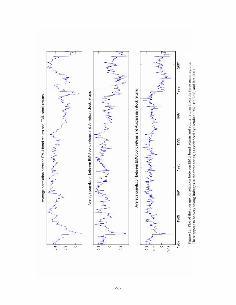
Finally, figures 12 and 13 contain plots of the average correlation between the various
equity markets and the EMU bond returns and American bond returns, respectively. Not
surprisingly, EMU bond returns are relatively highly correlated with EMU equity returns (Figure
12) while correlation between EMU bond returns and American and Australasian equity returns is
typically near zero and often negative, although both of these correlation remain in a relative
narrow band. If it has had any effect, the introduction of the Euro has led to a decrease in the
correlation between EMU bond returns and equity returns in other regions. One notable decrease
is evident in all three pictures: October 1987, providing strong evidence to a flight-to-quality.
The levels notwithstanding, the dynamics of the three series are remarkably similar, yet this
24 In fact, the decrease began slightly before the introduction of the fixed exchange rates. In the fourth week of October 1998, after months of carry trades involving borrowing at near zero interest rates in Japan, investing in the U.S., the Japanese central bank intervened against rising interest rates (while trying to encourage the economy) by buying bonds, causing the carry trade to unravel. In fact, the standardized return on Japanese bonds was 6 standard deviations this week.
-23-
similarity is most likely due to the equity return correlation dynamics. Figure 13 paints an
analogous picture for American bond returns, where the American bond returns have the highest
mean correlation with American equities (although similar to the mean with the EMU equities)
and have a much lower mean with Australasian equity returns. Again, the dynamics are similar
with all having a strong reaction in October 1987, and a slow but steady decline over the few
years.
VI. Conclusion
In this paper we found strong evidence of asymmetries in conditional covariance of both equity
and bond returns, although the asymmetries are present in markedly different manners.
Asymmetric DCC models are uniformly preferred to their symmetric counterparts using
likelihood ratio testing, and asset specific news impact curves and smoothing parameters to the
pooled parameter of a scalar DCC. While widespread evidence was found that national equity
index return series show asymmetry in conditional volatility, little evidence was found indicating
asymmetry in bond index return volatility. However, despite the lack of evidence of asymmetric
conditional volatilities, bonds (as well as equities) exhibit asymmetry in conditional correlation,
although, equities showed a stronger response to joint bad news than bonds do. Strong evidence
of market volatility correlation is also presented for equity returns: in particular, annualized
average volatility series for European, EMU, American and Australasian equities show linkages
during easily identifiable periods of financial turmoil such as the crash of ’87, the beginning o of
the Gulf war, and the Asian financial crisis. Again, unlike equity returns, bond market volatilities
demonstrate less clear linkages, instead, exhibiting increases to region specific events which do
not appear to be contagious across regions.
Upon the creation of the Euro, initially without a circulating currency when EMU
exchange rates were irrevocably fixed, significant evidence of a structural break is found in the
level of conditional correlation but not in the levels of the conditional volatilities. Conditional
equity correlation for the major markets of Europe, i.e. France, Germany and Italy (which are part
of the EMU) and UK (which is not part of the EMU), has increased since the introduction. In
addition to the expected increase in the Euro-area, evidence is also found of a meaningful
increase in correlation of other markets with the EMU nations, possibly signaling stronger
economic ties. Further, the introduction of a fixed exchange rate regime has led to near perfect
correlation among bond returns within EMU countries, which is not surprising in consideration of
the monetary policy harmonization within the EMU. This increase in correlation among asset
returns within the EMU area may have induced investors, when diversifying their portfolios, to
-24-
move capital from Europe to the US, possibly contributing to the depreciation of the euro vis-à-
vis the US dollar in the months following the introduction for the fixed rate regime.
Conditional equity correlation series among regional groups is found to increase
dramatically when bad news hit financial markets. This is am important implication for
international investors; diversification sought by investing in multiple markets is likely to be
lowest when it is most desirable. However, it is also evidenced that conditional correlation
between equity and bond returns usually declines when stock markets suffer from financial
turmoil, an indication of a “flight to quality phenomenon”, where investors move capital from
equities to safer assets. In other words, not only is equity-bond return correlation typically low, it
actually is lower during periods of financial turmoil. The findings of this paper have crucial
implications for practical international investing. While high correlation can become low
correlation by taking short positions, many large investors are prohibited or severely limited in
the amount of short position they may hold. Further, holding assets in a portfolio which may
have a negative expected return is typically undesirable. The lowest correlations found were
typically between equity returns in one country and bond returns in another. This unsurprising
yet undocumented observation should provide guidance for investors seeking to maximize
diversification without taking short positions.
The volatility and especially correlation dynamics documented in this paper raise
significant issues for both theoretical finance and investors. For instance, can the risk of
increasing correlation due to market declines (exactly when correlation becomes a very bad thing)
be hedged? Why do both equities and bonds demonstrate asymmetric changes in correlation
when they both decline? Has the introduction of the Euro fundamentally changed world equity
markets and how will this affect expected returns, capital flows, and exchange rates both within
and outside the Euro-area?
-25-
Appendix A: Historical background of the EMU
This appendix describes the essential steps which have led to the creation of the European
Monetary Union (EMU). After the collapse of the Bretton Wood system, in the spring 1972, the
European Economic Community (EEC) countries created the so-called “snake” in the “tunnel”:
EEC exchange rates were allowed to fluctuate within restricted margins (±1.125% - the snake)
around par value, but maintained wider margins (±2.25% - the tunnel) around the parities vis-à-
vis non-partner countries. Balance of payment difficulties led some countries to leave the snake
and the remaining members agreed, in March 1973, for a joint float: while maintaining fixed
parities with predetermined margins among themselves, they let their currencies float against the
US dollar. By 1975, however, the principle of somehow fixed exchange rates was dead.
A later attempt to create a currency area was undertaken in 1979, when the EEC countries
(except for Britain) created the European Monetary System (EMS), which was based on the
Exchange Rate Mechanism (ERM) and the European Currency Unit (ECU). As for the ERM,
once bilateral parities were declared, actual exchange rates could oscillate around them within
predefined margins (±2.25%, widened to ±15% from August 1993). Central parities could be
modified only by collective agreement and member countries were obliged to intervene in foreign
exchange markets when a margin was hit. The ECU differentiated the EMS from the old snake,
in that the creation of this common currency unit was the premise to a monetary union. The EMS
was characterized by broad exchange rate stability from January 1987 to August 1992, but also by
massive speculative attacks against the Italian lira, the British pound and the French Franc
(summer 1992 and 1993).
The Maastricht Treaty (signed in February 1992) laid out three stages which have led to
the EMU. In the first stage (1990-1993), which in fact started before the Treaty, several measures
were introduced, among which the abolition of restrictions to capital movements and the
prohibition of financing public deficit through central banks. The second stage (1994-6/8)
established, among other measures, a control of the public deficit (to be reduced to 3% of GDP)
and debt (to be not higher than 60% of GDP) as well as the constitution of the European
Monetary Institute (EMI), which was supposed to coordinate monetary policies. The second stage
was essentially designed to secure convergence of the EEC countries and allow the introduction
of a single currency. Member participants were supposed to meet a number of convergence
criteria, among which: an inflation rate not larger than 1.5% the inflation rate of the three best
performing countries, i.e. those with the lowest inflation rates; a long-term interest rate not larger
than 2% the average interest rate of those same three countries; an exchange rate within the
-26-
fluctuation margins in the last two years. In the third stage, which begun in January 1999, the
European Central Bank (ECB) was created, bilateral exchange rates were irrevocably fixed and
the euro has been replacing the single national currencies. On January 1 1999 bilateral exchange
rates between member countries were irrevocably fixed (as well as those vis-à-vis the ECU),
while the European single currency changed its name from ECU into euro. The euro, which first
was a non-circulating currency, began to circulate from January 1 2002, and it will be totally
replacing the national currencies from July 1 2002 at the latest.25
25 The countries which are part of the European Monetary Union are: Austria, Belgium, Finland, France, Germany, Greece, Ireland, Italy, Luxembourg, the Netherlands, Portugal, and Spain.
-27-
Appendix B: Countries Selected
Australasia
• AUSTRALIA
• HONG KONG
• JAPAN*
• NEW ZEALAND
• SINGAPORE
Europe
• AUSTRIA*
• BELGIUM*
• DENMARK*
• FRANCE*
• GERMANY*
• IRELAND*
• ITALY
• THE NETHERLANDS*
• SPAIN
• SWEDEN*
• SWITZERLAND*
• NORWAY
• UNITED KINGDOM*
Americas
• CANADA*
• MEXICO
• UNITED STATES*
* indicates bond data included for these countries.
-28-
Appendix C: Exact Specifications
C.1 Univariate GARCH models
While some of the models differ in the exact representation originally proposed, the qualitative
features remain unchanged. The models were changed to improve comparability across models.
GARCH
12
1 −− ++= ttt hh βαεω
AVGARCH (Absolute Value)
2/111
2/1 || −− ++= ttt hh βεαω
NARCH (Non-linear) 2/
112/ || λλλ βεαω −− ++= ttt hh
EGARCH (Exponential)
)log(||
)log( 11
1
1
1−
−
−
−
− +++= tt
t
t
tt h
hhh β
εγ
εαω
ZARCH (Threshold) 2/11111
2/1 ||]0[|| −−−− +<++= ttttt hIh βεεγεαω
GJR-GARCH
12
112
1 ]0[ −−−− +<++= ttttt hIh βεεγαεω
APARCH (Asymmetric Power)
2/1111
2/ ||]0[|| λλλλ βεεγεαω −−−− +<++= ttttt hIh
AGARCH (Asymmetric)
12
1 )( −− +++= ttt hh βγεαω
NAGARCH (Nonlinear Asymmetric)
12
11 )( −−− +++= tttt hhh βγεαω
-29-
C. 2 New Impact Surface for correlation
0,,)~)(~(
~),(
0,0,))(~)(~(
~),(
0,0,)~)()(~(
~),(
0,,))(~)()(~(
)(~),(
21222222
,21
212222222
,21
212222222
,21
2122222222
,21
>++++
++=
<>+++++
++=
><+++++
++=
<++++++
+++=
eeforbeacbeac
bbeeaaceef
eeforbegacbeac
bbeeaaceef
eeforbeacbegac
bbeeaaceef
eeforbegacbegac
bbeeggaaceef
iiiijiiiii
tijjijijiij
jjjjjjiiiii
tijjijijiij
jjjjjiiiiii
tijjijijiij
jjjjjjiiiiii
tijjijijijiij
ρ
ρ
ρ
ρ
-30-
Bibliography Ang, A. and G. Bekaert, 1999, "International Asset Allocation with Time-Varying Correlations," NBER
Working Papers 7056, National Bureau of Economic Research, Inc. 1999.
Bekaert, G, and G. Wu, 2000, "Asymmetric Volatility and Risk in Equity Markets," Review of Financial
Studies, Vol. 13 (1), pp. 1-42.
Black, F., 1976, “Studies of Stock Prices Volatility Changes,” Proceeding from the American Statistical
Association, Business and Economics Statistics Section, pp. 177-181.
Bollerslev, T., 1986, "Generalized Autoregressive Conditional Heteroskedasticity," Journal of
Econometrics, Vol.31, pp.307-327.
Bollerslev, T, 1990, "Modeling the Coherence in Short Run Nominal Exchange Rates: A Multivariate
Generalized ARCH Model," Review of Economics and Statistics, Vol.72, No.3, pp.498-505.
Booth, G. G., T. Martikainen, and Y. Tse, 1997, "Price and Volatilities Spillovers in Scandinavian Stock
Markets", Journal of International Money and Finance, Vol. 21, June, 811-823.
Braun, P. A., D. B. Nelson, and A. M. Sunier, 1995, “Good News, Bad News, Volatility, and Betas,”
Journal of Finance, 50, pp. 1575-1603.
Brooks, C., and U. T. Henry, 2000, “Linear and Non-Linear Transmission of Equity Return Volatility:
Evidence from the US, Japan and Australia,” Economic Modeling , 174, pp. 497-513.
Campbell, J. Y., and L. Hentschell, 1992, “No News Is Good News,” Journal of Financial Economics, 31,
pp. 281-318.
Cappiello, L., 2000, “Do Fixed Income Securities Also Show Asymmetric Effects in Conditional Second
Moments?,” FAME working paper, # 12, Geneva, Switzerland.
Christiansen, C., 2000, “Macroeconomic Announcement Effects on the Covariance Structure of
Government Bond Returns,” Journal of Empirical Finance, 75, pp. 479-507.
Christie, A., 1982, “The Stochastic Behavior of Common Stock Variances,” Journal of Financial
Economics, 10, 407-432.
Das, S., and R. Uppal, 2001, “Systemic risk and international portfolio choice,” Manuscript, Harvard
University.
De Santis, G. and B. Gerard, 1997, “International Asset Pricing and Portfolio Diversification with Time-
Varying Risk,” Journal of Finance, 52, 1881-1912.
Ding, Z., R. F. Engle and C.W.J. Granger, 1993, "A Long Memory Property of Stock Market Returns and a
New Model," Journal of Empirical Finance, Vol. 1, pp. 83-106.
-31-
Engle, R. F., 1982, "Autoregressive Conditional Heteroskedasticity with Estimates of the Variance of U.K.
Inflation," Econometrica. Vol. 50, pp. 987-1008.
Engle, R. F., 2002, "Dynamic Conditional Correlation - A Simple Class of Multivariate GARCH Models,"
Forthcoming in Journal of Business and Economic Statistics.
Engle, R. F., and L. Li, 1998, "Macroeconomic Announcements and Volatility of Treasury Futures," UCSD
Working Paper No. 97-27.
Engle, R. F., and V. Ng, 1993, "Measuring and Testing the Impact of News On Volatility," Journal of
Finance, Vol. 48, pp. 1749-78.
Engle, R. F., and K. Sheppard, 2001, “Theoretical and Empirical Properties of Dynamic Conditional
Correlation MVGARCH”, UCSD Working Paper No. 2001-15.
Erb, C., C. R. Harvey, and T. Viskanta, 1994, “National Risk and Global Fixed Income Allocation,”
Journal of Fixed Income , pp. 17-26.
Errunza, V., K. H. and M.-W. Hung, “Can the Gains from International Diversification be Achieved without
Trading Abroad?,” Journal of Finance, 1999, Vol. 54, pp. 2075-2107.
Glosten, L., R. Jagannathan, and D. Runkle, 1993, "Relationship Between the Expected Value and the
Volatility of the Nominal Excess Return on Stocks," Journal of Finance, Vol. 48, pp. 1779-1801.
Hansen, P. R., and A. Lunde, 2001, “A Forecast Comparison of Volatility Models: Does Anything Beat a
GARCH(1,1),” Brown University Working Paper No. 01-04.
Hentschel, L., 1995, "All in the family: Nesting symmetric and asymmetric GARCH models," Journal of
Financial Economics, Vol. 39, pp. 71-104.
Higgins, M. L., and A. K. Bera, 1992, “A Class of Nonlinear ARCH Models,” International Economic
Review, 33, pp. 137-158.
Isakov D. and C. Pérignon, 2000, "On the dynamic interdependence of international stock markets : A
Swiss perspective," Swiss Journal of Economics and Statistics, Vol. 136, No. 2, pp. 123-146.
Koutmos, G., and G. G. Booth, 1995, “Asymmetric Volatility Transmission in International Stock
Markets,” Journal of International Money and Finance. Vol. 14, No. 6, pp. 747-62.
Koutmos, G., 1996, “Modeling the Dynamic Interdependence of Major European Stock Markets,” Journal
of Business, Finance, and Accounting, 23, pp. 975-988.
Kroner, K. F., and V. K. Ng, 1998, “Modeling asymmetric comovements of assets returns,” Review of
Financial Studies. Vol. 11, No.4, pp 817-44.
Jones, C., O. Lamont, and R. Lumsdaine, 1998, "Macroeconomic News and Bond Market Volatility,"
Journal of Financial Economics. March, pp. 315-27.
-32-
Longin, F., and B. Solnik, 2002, “Extreme Correlation of International Equity Markets,” Forthcoming in
The Journal of Finance.
Marten, M. and S.-H. Poon, 2001, “Return Synchronization and daily correlation dynamics between
international stock markets,” Journal of Banking and Finance , Vol. 25, pp. 1805-27.
Moskowitz, T., 2002, “An Analysis of Covariance Risk and Pricing Anomalies,” Manuscript, Graduate
School of Business, University of Chicago.
Nelson, D. B., 1991, “Conditional Heteroskedasticity in Asset Returns: A new approach,” Econometrica,
Vol. 59, pp. 347-70.
Patton, A. 2001, “On the Importance of Skewness and Asymmetric Dependence in Stock Returns for Asset
Allocation,” Manuscript, UCSD.
Scruggs, John T., 1998, “Resolving the Puzzling Intertemporal Relation between the Market Risk Premium
and Conditional Market Variance: A Two-Factor Approach,” Journal of Finance, Vol. 53, pp. 575-
603.
Sheppard, K., 2002, “Understanding the Dynamics of Equity Covariance,” Manuscript, UCSD.
Taylor, S. J., 1986, Modeling Financial Time Series, John Wiley and Sons Ltd.
Wooldridge, J, 1991, “On the application of robust, regression based diagnostics to models of conditional
means and conditional variances”, Journal of Econometrics, Vol. 47, pp 5-46.
Table 2b: Unconditional correlation of returns across the equity (down) and bond markets (across). Red numbers indicate negative correlation. For instance, the upper left entry is the correlation between Australian equity returns and Austrian bond returns. Immediately below this entry is the correlation between Austrian equity returns and Austrian bond returns.
Table 3
Overall Intra-stock Intra-bond Interstock Bond Significant at 10% 0.146 0.291 0.077 0.055 Significant at 20% 0.292 0.552 0.154 0.132 Stocks Only Significant at 20% Australasia Europe North America Australasia 0.500 Europe 0.323 0.333 North America 0.133 0.180 0.000 Bonds only Significant at 20% Australasia Europe North America Australasia - Europe 0.000 0.133 North America 0.000 0.000 0.000 Across Stocks - Bonds Significant at 20% Stocks Australasia Europe North America Australasia 0.000 0.000 0.000 Bonds Europe 0.020 0.069 0.033 North America 0.100 0.000 0.500
Table 3: Summary Statistics for conditional partial correlation. The numbers represent the
percentage of the series rejecting the null that the conditional partial correlation is the same after
joint bad news(two negative returns) as it as after joint good news(two positive returns). Except
where explicitly indicated, all tests were at the 10% level.
Belgium Canada Denmark France Germany Ireland Japan Neth'l Sweden Switz'l U. K. U. S. Austria 0.914 0.070 0.884 0.896 0.950 0.809 0.441 0.947 0.647 0.844 0.626 0.186 Belgium 0.094 0.898 0.909 0.939 0.814 0.455 0.940 0.667 0.832 0.643 0.207 Canada 0.094 0.097 0.068 0.134 0.007 0.082 0.160 -0.019 0.167 0.452 Denmark 0.907 0.909 0.839 0.418 0.908 0.696 0.800 0.650 0.195 France 0.927 0.832 0.428 0.933 0.679 0.823 0.673 0.267 Germany 0.826 0.464 0.984 0.657 0.866 0.656 0.221 Ireland 0.359 0.835 0.664 0.710 0.699 0.212 Japan 0.458 0.294 0.475 0.343 0.038 Neth'l 0.667 0.861 0.657 0.234 Sweden 0.553 0.566 0.173 Switz'l 0.589 0.126 U. K. 0.249
Table 2c
Table 2c: Unconditional correlation of returns across the bond returns. Red numbers indicate negative correlation.
-35-
Table 4
Table 4: Summary Statistics for the 21 Equity Index returns and 13 Bond Index returns. The
standardized skewness and standardized kurtosis are the skewness and kurtosis of the returns
standardized by their estimated standard deviation. (§ denotes Annualized Percent, * denotes
standardized residuals insignificantly different from a normal distribution at 5%, ** at 1%)
Mean§ Standard
Dev.§ Skewness Kurtosis Standardized
Skewness Standardized
Kurtosis Australia Stocks 9.10 20.49 -2.23 24.33 -1.26 12.25