Georgian Mathematical Journal Volume 7 (2000), Number 1, 11-32 ASYMPTOTIC DISTRIBUTION OF EIGENELEMENTS OF THE BASIC TWO-DIMENSIONAL BOUNDARY-CONTACT PROBLEMS OF OSCILLATION IN CLASSICAL AND COUPLE-STRESS THEORIES OF ELASTICITY T. BURCHULADZE AND R. RUKHADZE Abstract. The basic boundary-contact problems of oscillation are consi- dered for a two-dimensional piecewise-homogeneous isotropic elastic medium bounded by several closed curves. Asymptotic formulas for the distribution of eigenfunctions and eigenvalues of the considered problems are derived using the correlation method. 1. In this paper the following notation will be used: R 2 is a two-dimensio- nal Euclidean space; x =(x 1 ,x 2 ), y =(y 1 ,y 2 ) are points in R 2 ; |x - y| is the Euclidean distance between x and y; D 0 ⊂ R 2 is a finite domain bounded by the closed curves S 0 ,S 1 ,...,S m of the class Λ 2 (α), 0 <α ≤ 1 (the curves have a H¨older-continuous curvature), S 0 is enveloping all other S k , while the latters are not enveloping one another, S i ∩ S k = ∅ for i 6= k, i, k = 0,m; the finite domain bounded by the curve S k (k = 1,m) is denoted by D k , D 0 = D 0 ∪ ( m ∪ k=0 S k ), D k = D k ∪ S k , k = 1,m. If u and v are the n-component real-valued vectors u =(u 1 ,u 2 ,...,u n ), v =(v 1 ,v 2 ,...,v n ), then uv denotes the scalar product of these vectors: uv = n ∑ k=1 u k v k ; |u| =( n ∑ k=1 u 2 k ) 1/2 . The matrix product is obtained by multiplying a row vector by a column vector; if A = kA ij k n×n is an n × n-matrix, then |A| 2 = n ∑ i,j =1 A 2 ij . Any vector u =(u 1 ,u 2 ,...,u n ) is considered as an n × 1 one- column matrix: u = ku i k n×1 ; A k = kA jk k n j =1 is the k-th column vector of the matrix A. The vector u(x)=(u 1 (x),u 2 (x),...,u n (x)) is called regular in D k if u i ∈ C 1 (D k ) ∩ C 2 ( D k ), i = 1,n. A system of homogeneous differential equations of oscillation of the classical 2000 Mathematics Subject Classification. 74B05. Key words and phrases. Oscillation of piecewise-homogeneous isotropic elastic medium, asymptotic distribution of eigenelements, Carleman method. ISSN 1072-947X / $8.00 / c Heldermann Verlag www.heldermann.de
Transcript
Georgian Mathematical JournalVolume 7 (2000), Number 1, 11-32
ASYMPTOTIC DISTRIBUTION OF EIGENELEMENTS OFTHE BASIC TWO-DIMENSIONAL BOUNDARY-CONTACT
PROBLEMS OF OSCILLATION IN CLASSICAL ANDCOUPLE-STRESS THEORIES OF ELASTICITY
T. BURCHULADZE AND R. RUKHADZE
Abstract. The basic boundary-contact problems of oscillation are consi-dered for a two-dimensional piecewise-homogeneous isotropic elastic mediumbounded by several closed curves. Asymptotic formulas for the distribution ofeigenfunctions and eigenvalues of the considered problems are derived usingthe correlation method.
1. In this paper the following notation will be used: R2 is a two-dimensio-nal Euclidean space; x = (x1, x2), y = (y1, y2) are points in R2; |x − y| is theEuclidean distance between x and y; D0 ⊂ R2 is a finite domain bounded bythe closed curves S0, S1, . . . , Sm of the class Λ2(α), 0 < α ≤ 1 (the curves have aHolder-continuous curvature), S0 is enveloping all other Sk, while the latters arenot enveloping one another, Si∩Sk = ∅ for i 6= k, i, k = 0,m; the finite domainbounded by the curve Sk (k = 1, m) is denoted by Dk, D0 = D0 ∪ (
m∪
k=0Sk),
Dk = Dk ∪ Sk, k = 1,m.If u and v are the n-component real-valued vectors u = (u1, u2, . . . , un),
v = (v1, v2, . . . , vn), then uv denotes the scalar product of these vectors: uv =n∑
k=1ukvk; |u| = (
n∑
k=1u2
k)1/2. The matrix product is obtained by multiplying a
row vector by a column vector; if A = ‖Aij‖n×n is an n × n-matrix, then
|A|2 =n∑
i,j=1A2
ij. Any vector u = (u1, u2, . . . , un) is considered as an n × 1 one-
column matrix: u = ‖ui‖n×1; Ak = ‖Ajk‖nj=1 is the k-th column vector of the
matrix A.The vector u(x) = (u1(x), u2(x), . . . , un(x)) is called regular in Dk if ui ∈
C1(Dk) ∩ C2(Dk), i = 1, n.A system of homogeneous differential equations of oscillation of the classical
2000 Mathematics Subject Classification. 74B05.Key words and phrases. Oscillation of piecewise-homogeneous isotropic elastic medium,
asymptotic distribution of eigenelements, Carleman method.
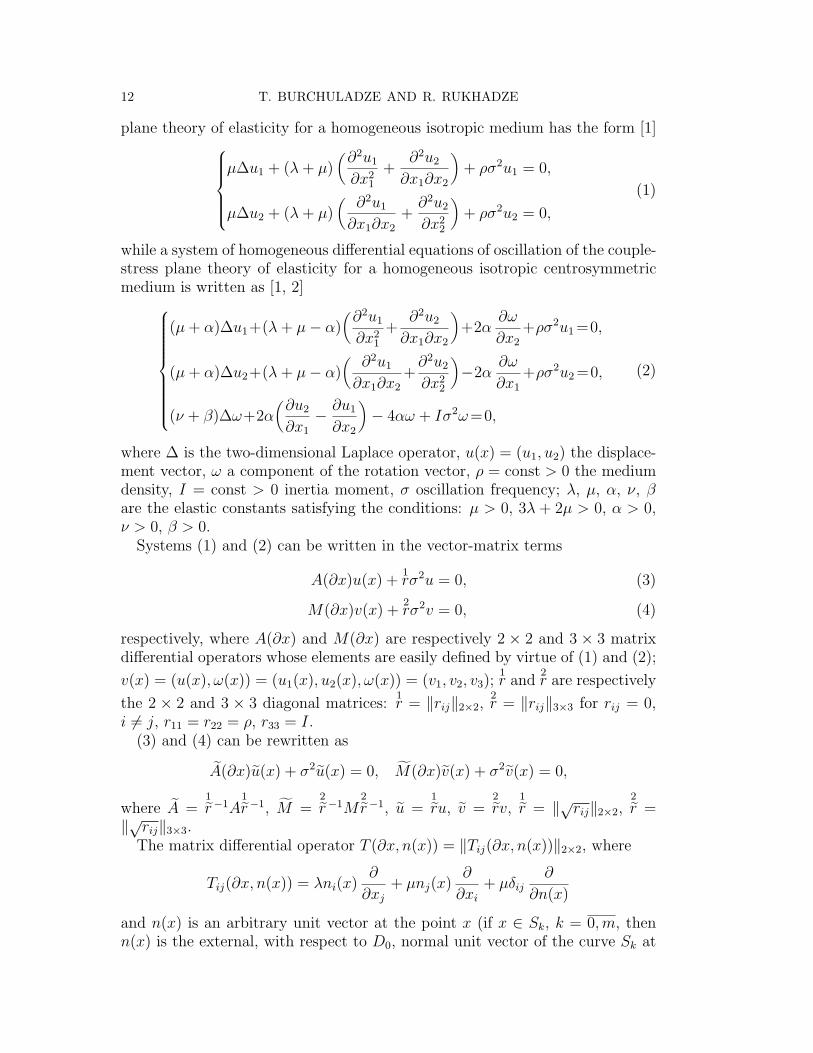
plane theory of elasticity for a homogeneous isotropic medium has the form [1]
µ∆u1 + (λ + µ)(∂2u1
∂x21
+∂2u2
∂x1∂x2
)
+ ρσ2u1 = 0,
µ∆u2 + (λ + µ)( ∂2u1
∂x1∂x2+
∂2u2
∂x22
)
+ ρσ2u2 = 0,(1)
while a system of homogeneous differential equations of oscillation of the couple-stress plane theory of elasticity for a homogeneous isotropic centrosymmetricmedium is written as [1, 2]
(µ + α)∆u1+(λ + µ− α)(∂2u1
∂x21
+∂2u2
∂x1∂x2
)
+2α∂ω∂x2
+ρσ2u1 =0,
(µ + α)∆u2+(λ + µ− α)( ∂2u1
∂x1∂x2+
∂2u2
∂x22
)
−2α∂ω∂x1
+ρσ2u2 =0,
(ν + β)∆ω+2α(∂u2
∂x1− ∂u1
∂x2
)
− 4αω + Iσ2ω=0,
(2)
where ∆ is the two-dimensional Laplace operator, u(x) = (u1, u2) the displace-ment vector, ω a component of the rotation vector, ρ = const > 0 the mediumdensity, I = const > 0 inertia moment, σ oscillation frequency; λ, µ, α, ν, βare the elastic constants satisfying the conditions: µ > 0, 3λ + 2µ > 0, α > 0,ν > 0, β > 0.
Systems (1) and (2) can be written in the vector-matrix terms
A(∂x)u(x) + 1rσ2u = 0, (3)
M(∂x)v(x) + 2rσ2v = 0, (4)
respectively, where A(∂x) and M(∂x) are respectively 2 × 2 and 3 × 3 matrixdifferential operators whose elements are easily defined by virtue of (1) and (2);v(x) = (u(x), ω(x)) = (u1(x), u2(x), ω(x)) = (v1, v2, v3);
1r and 2r are respectivelythe 2 × 2 and 3 × 3 diagonal matrices: 1r = ‖rij‖2×2,
2r = ‖rij‖3×3 for rij = 0,i 6= j, r11 = r22 = ρ, r33 = I.
(3) and (4) can be rewritten as
˜A(∂x)u(x) + σ2u(x) = 0, ˜M(∂x)v(x) + σ2v(x) = 0,
where ˜A =1r−1A
1r−1, ˜M =
2r−1M
2r−1, u =
1ru, v =
2rv,
1r = ‖√rij‖2×2,
2r =
‖√rij‖3×3.The matrix differential operator T (∂x, n(x)) = ‖Tij(∂x, n(x))‖2×2, where
Tij(∂x, n(x)) = λni(x)∂
∂xj+ µnj(x)
∂∂xi
+ µδij∂
∂n(x)
and n(x) is an arbitrary unit vector at the point x (if x ∈ Sk, k = 0,m, thenn(x) is the external, with respect to D0, normal unit vector of the curve Sk at
ASYMPTOTIC DISTRIBUTION OF EIGENELEMENTS 13
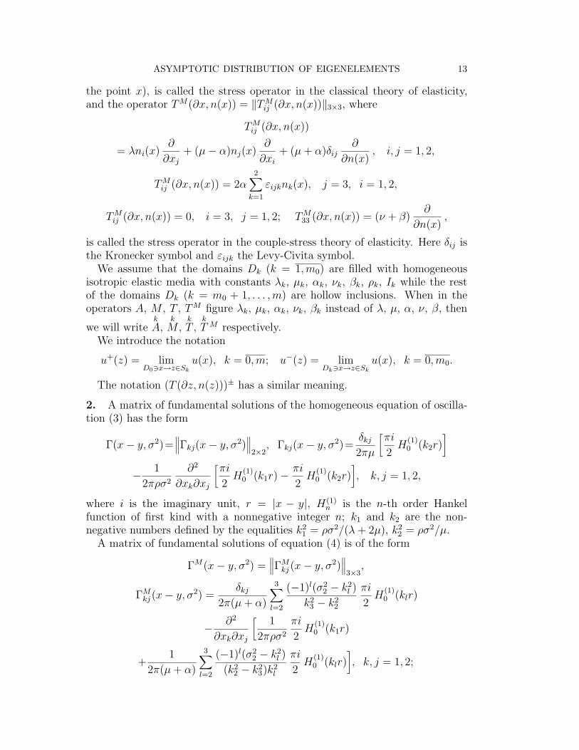
the point x), is called the stress operator in the classical theory of elasticity,and the operator TM(∂x, n(x)) = ‖TM
ij (∂x, n(x))‖3×3, where
TMij (∂x, n(x))
= λni(x)∂
∂xj+ (µ− α)nj(x)
∂∂xi
+ (µ + α)δij∂
∂n(x), i, j = 1, 2,
TMij (∂x, n(x)) = 2α
2∑
k=1
εijknk(x), j = 3, i = 1, 2,
TMij (∂x, n(x)) = 0, i = 3, j = 1, 2; TM
33 (∂x, n(x)) = (ν + β)∂
∂n(x),
is called the stress operator in the couple-stress theory of elasticity. Here δij isthe Kronecker symbol and εijk the Levy-Civita symbol.
We assume that the domains Dk (k = 1,m0) are filled with homogeneousisotropic elastic media with constants λk, µk, αk, νk, βk, ρk, Ik while the restof the domains Dk (k = m0 + 1, . . . , m) are hollow inclusions. When in theoperators A, M , T , TM figure λk, µk, αk, νk, βk instead of λ, µ, α, ν, β, then
we will writekA,
kM ,
kT ,
kT M respectively.
We introduce the notation
u+(z) = limD03x→z∈Sk
u(x), k = 0,m; u−(z) = limDk3x→z∈Sk
u(x), k = 0,m0.
The notation (T (∂z, n(z)))± has a similar meaning.
2. A matrix of fundamental solutions of the homogeneous equation of oscilla-tion (3) has the form
Γ(x− y, σ2)=∥
∥
∥Γkj(x− y, σ2)∥
∥
∥
2×2, Γkj(x− y, σ2)=
δkj
2πµ
[πi2
H(1)0 (k2r)
]
− 12πρσ2
∂2
∂xk∂xj
[πi2
H(1)0 (k1r)−
πi2
H(1)0 (k2r)
]
, k, j = 1, 2,
where i is the imaginary unit, r = |x − y|, H(1)n is the n-th order Hankel
function of first kind with a nonnegative integer n; k1 and k2 are the non-negative numbers defined by the equalities k2
1 = ρσ2/(λ + 2µ), k22 = ρσ2/µ.
A matrix of fundamental solutions of equation (4) is of the form
ΓM(x− y, σ2) =∥
∥
∥ΓMkj (x− y, σ2)
∥
∥
∥
3×3,
ΓMkj (x− y, σ2) =
δkj
2π(µ + α)
3∑
l=2
(−1)l(σ22 − k2
l )k2
3 − k22
πi2
H(1)0 (klr)
− ∂2
∂xk∂xj
[ 12πρσ2
πi2
H(1)0 (k1r)
+1
2π(µ + α)
3∑
l=2
(−1)l(σ22 − k2
l )(k2
2 − k23)k2
l
πi2
H(1)0 (klr)
]
, k, j = 1, 2;
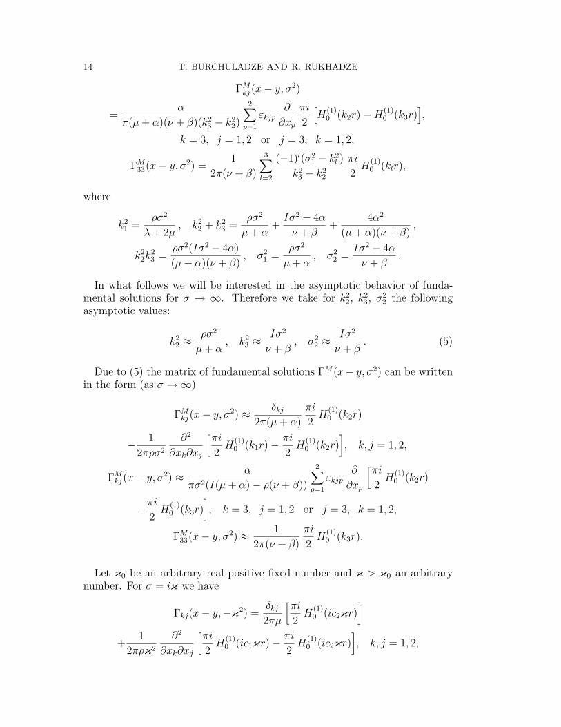
14 T. BURCHULADZE AND R. RUKHADZE
ΓMkj (x− y, σ2)
=α
π(µ + α)(ν + β)(k23 − k2
2)
2∑
p=1εkjp
∂∂xp
πi2
[
H(1)0 (k2r)−H(1)
0 (k3r)]
,
k = 3, j = 1, 2 or j = 3, k = 1, 2,
ΓM33(x− y, σ2) =
12π(ν + β)
3∑
l=2
(−1)l(σ21 − k2
l )k2
3 − k22
πi2
H(1)0 (klr),
where
k21 =
ρσ2
λ + 2µ, k2
2 + k23 =
ρσ2
µ + α+
Iσ2 − 4αν + β
+4α2
(µ + α)(ν + β),
k22k
23 =
ρσ2(Iσ2 − 4α)(µ + α)(ν + β)
, σ21 =
ρσ2
µ + α, σ2
2 =Iσ2 − 4α
ν + β.
In what follows we will be interested in the asymptotic behavior of funda-mental solutions for σ → ∞. Therefore we take for k2
2, k23, σ2
2 the followingasymptotic values:
k22 ≈
ρσ2
µ + α, k2
3 ≈Iσ2
ν + β, σ2
2 ≈Iσ2
ν + β. (5)
Due to (5) the matrix of fundamental solutions ΓM(x− y, σ2) can be writtenin the form (as σ →∞)
ΓMkj (x− y, σ2) ≈ δkj
2π(µ + α)πi2
H(1)0 (k2r)
− 12πρσ2
∂2
∂xk∂xj
[πi2
H(1)0 (k1r)−
πi2
H(1)0 (k2r)
]
, k, j = 1, 2,
ΓMkj (x− y, σ2) ≈ α
πσ2(I(µ + α)− ρ(ν + β))
2∑
ρ=1εkjp
∂∂xp
[πi2
H(1)0 (k2r)
−πi2
H(1)0 (k3r)
]
, k = 3, j = 1, 2 or j = 3, k = 1, 2,
ΓM33(x− y, σ2) ≈ 1
2π(ν + β)πi2
H(1)0 (k3r).
Let κ0 be an arbitrary real positive fixed number and κ > κ0 an arbitrarynumber. For σ = iκ we have
Γkj(x− y,−κ2) =δkj
2πµ
[πi2
H(1)0 (ic2κr)
]
+1
2πρκ2
∂2
∂xk∂xj
[πi2
H(1)0 (ic1κr)− πi
2H(1)
0 (ic2κr)]
, k, j = 1, 2,
ASYMPTOTIC DISTRIBUTION OF EIGENELEMENTS 15
where
c21 =
ρλ + 2µ
, c22 =
ρµ
,
ΓMkj (x− y,−κ2) =
δkj
2π(µ + α)
[πi2
H(1)0 (ic2κr)
]
+1
2πρκ2
∂2
∂xk∂xj
[πi2
H(1)0 (ic1κr)− πi
2H(1)
0 (ic2κr)]
, k, j = 1, 2,
ΓMkj (x− y,−κ2)
= − απκ2(I(µ + α)− ρ(ν + β))
2∑
p=1εkjp
∂∂xp
[πi2
H(1)0 (ic2κr)
−πi2
H(1)0 (ic3κr)
]
, k = 3, j = 1, 2 or j = 3, k = 1, 2,
ΓM33(x− y,−κ2) =
12π(ν + β)
[πi2
H(1)0 (ic3κr)
]
,
where c21 = ρ
λ+2µ , c22 = ρ
µ+α , c23 = I
ν+β .We will consider two possible cases:1. κr is bounded for r → 0 and κ →∞;2. κr is unbounded for r → 0 and κ →∞.When κr is bounded, taking into account repersentations of the Hankel func-
tion, we have
|Γpq(x− y,−κ2)| ≤ const | lnκr|,∣
∣
∣
∣
∂nΓpq(x− y,−κ2)∂xi
1∂xj2
∣
∣
∣
∣
≤ constrn , (6)
i + j = n, n = 1, 2, . . . ; p, q = 1, 2.
The same estimates are obtained for ΓMpq (x− y,−κ2).
When κr is unbounded, we use the asymptotic representation of the Hankelfunction for large |z| [3]
H(1)n (z) =
√
2πz
ei(z−n π2−
π4 )
[
1 + O(1
z
)]
,
and the recurrent formula [3] 2 ddz H(1)
n (z) = H(1)n−1(z)−H(1)
n+1(z), to obtain
∣
∣
∣
∣
∂nΓpq(x− y,−κ2)∂xi
1∂xj2
∣
∣
∣
∣
≤ constκn
√κr
e−a{r, (7)
i + j = n, n = 0, 1, 2, . . . ; p, q = 1, 2,
where a = c1 − δ > 0, δ < 12 c1 is an arbitrary positive number;
∣
∣
∣
∣
∂nΓMpq (x− y,−κ2)
∂xi1∂xj
2
∣
∣
∣
∣
≤ constκn
√κr
e−b{r,
16 T. BURCHULADZE AND R. RUKHADZE
where b = c∗ − δ, δ < 12 c∗ is an arbitrary positive number, c∗ is the smallest of
the numbers c1, c2, c3.
3. Let x, y ∈ Dk, k = 0, m0 and ly be the distance from the point y to theboundary of the domain Dk. We denote ρy(x) = max{r, ly} and introduce theauxiliary matrix
kΓ(x− y,−κ2) =
[
1−(
1− rm
ρmy (x)
)n] kΓ(x− y,−κ2). (8)
Let us denote by K(y, ly) the circle of radius ly and center at the point y,and by C(y, ly) the boundary of this circle. We easily find that (1−rm/ρm
y (x))n
vanishes together with its derivatives up to (n − 1)-th order inclusive whenthe point x ∈ K(y, ly) tends to a point of the boundary C(y, ly). For x ∈Dk\K(y, ly) we have 1− (1− rm/ρm
y (x))n = 1 and
limK(y,ly)3x→z∈C(y,ly)
[
1−(
1− rm
ρmy (x)
)n]
= 1.
ThereforekΓ(x − y,−κ2) =
kΓ(x − y,−κ2) for x ∈ Dk\K(y, ly), while, in
crossing the boundary C(y, ly), the functionkΓ and its derivatives up to (n−1)-
th order inclusive remain continuous.
We write the functionkΓ in the form
kΓ(x− y,−κ2) =
kΓ(x− y,−κ2)
(
nrm
ρmy (x)
+ . . .)
.
It is easy to verify that for x = y the functionkΓ and its derivatives up to
(m − 2)-th order inclusive are continuous. By virtue of (6), for x ∈ K(y, ly),when κr is bounded, we have the estimates
∣
∣
∣
kΓpq(x− y,−κ2)
∣
∣
∣ ≤ const rm−α
καlmy,
∣
∣
∣
∣
∂skΓpq(x− y,−κ2)
∂xi1∂xj
2
∣
∣
∣
∣
≤ const rm−s
lmy, (9)
i + j = s; m ≥ s + 1, p, q = 1, 2,
where α is an arbitrary number, 0 < α < 1.When κr is unbounded, by virtue of (7) we have the estimates
∣
∣
∣
∣
∂skΓpq(x− y,−κ2)
∂xi1∂xj
2
∣
∣
∣
∣
≤ constκse−a{r
√κlmy
rm− 12 . (10)
Analogous estimates hold forkΓM(x− y,−κ2).
ASYMPTOTIC DISTRIBUTION OF EIGENELEMENTS 17
4. Let us calculate the limit
limx→y
[ kΓ(x− y,−κ2)−
kΓ(x− y,−κ2
0)]
, x, y ∈ Dk, k = 0, m0.
Using the expansion
H(1)0 (z) = I0(z) +
2iπ
I0(z) lnz2− 2i
π
∞∑
k=0
(−1)k
(k!)2
(z2
)2k(
1 +12
+ · · ·+ 1k− γ
)
,
where γ is the Euler’s constant,
I0(z) =∞∑
k=0
(−1)k
(k!)2
(z2
)2k= 1− z2
22(1!)2 +z4
24(2!)2 −z6
26(3!)2 + · · · ,
I0(ic1κr)− I0(ic2κr) =κ2(c2
1 − c22)
22(1!)2 r2 +κ4(c4
1 − c42)
24(2!)2 r4 − · · ·
and the following evident relations
∂2r2
∂xk∂xj= 2δkj , ln
ic1κr2
= lnic1
2+ lnκ + ln r,
for p, q = 1, 2 we have
limx→y
[ kΓpq(x− y,−κ2)−
kΓpq(x− y,−κ2
0)]
=1
2πµkδpq ln
κ0
κ
+14π
δpq
( 1λk + 2µk
− 1µk
)
lnκ0
κ =14π
( 1λk + 2µk
+1µk
)
δpq lnκ0
κ . (11)
Quite similarly, we obtain
limx→y
[ kΓM
pq (x− y,−κ2)−kΓM
pq (x− y,−κ20)
=14π
( 1λk + 2µk
+1
µk + αk
)
δpq lnκ0
κ , p, q = 1, 2,
limx→y
[ kΓM
33(x− y,−κ2)−kΓM
33(x− y,−κ20)
]
=12π
1νk + βk
lnκ0
κ .
(12)
5. Further we will investigate the first problem. The other problems are con-sidered similarly.
The 2 × 2 matrix G(x, y,−κ20) =
kG(x, y,−κ2
0), x ∈ Dk, y ∈ D =m0∪k=0
Dk,
x 6= y, k = 0,m0, denotes the Green tensor of the first basic boundary value
problem of the operatorkA(∂x)− κ2
0E (E is the 2× 2 unit matrix).According to [4], G(x, y,−κ2
0) possesses a symmetry property of the form
G(x, y,−κ20) = G>(y, x,−κ2
0), (13)
18 T. BURCHULADZE AND R. RUKHADZE
where the symbol > denotes the matrix transposition operation. Moreover, weobtain the estimates [5]
∀(x, y) ∈ Dk ×Dk : Gpq(x, y,−κ20) = O
(
| ln |x− y| |)
,
∂∂xj
Gpq(x, y,−κ20) = O(|x− y|−1), p, q, j = 1, 2, k = 0,m0.
(14)
In a similar way we can define the Green tensor of the first basic boundary-
contact problem of the operatorkM(∂x) − κ2
0E (E is the 3 × 3 unit matrix)GM(x, y,−κ2
0) which is of size 3×3. This tensor has property (13) and estimates(14) hold for it.
6. Let u(x) = ku(x) and v(x) = kv(x), x ∈ Dk be arbitrary regular vectors ofthe class C1(Dk) ∩ C2(Dk). Then we have the Green formula [4]
m0∑
k=0
∫
Dk
[kvkAku +
kE(kv, ku)
]
dx
=∫
S
0v+(0T 0u)+ dS +
m0∑
k=1
∫
Sk
[0v+(0T 0u)+ − kv−(
kT ku)−
]
dS, (15)
where S = S0 ∪ (m∪
k=m0+1Sk) and
kE(kv, ku) =
2∑
p,q=1
(
µk∂ kvp
∂xq
∂ kup
∂xq+ λk
∂ kvp
∂xq
∂ kuq
∂xq+ µk
∂ kvp
∂xq
∂ kuq
∂xp
)
. (16)
We can rewrite (16) as
kE(kv, ku) =
3λk + 2µk
3
(∂ kv1
∂x1+
∂ kv2
∂x2
)(∂ ku1
∂x1+
∂ ku2
∂x2
)
+µk
2
∑
p 6=q
(∂ kvp
∂xq+
∂ kvq
∂xp
)(∂ kup
∂xq+
∂ kuq
∂xp
)
+µk
3
∑
p, q
(∂ kvp
∂xp− ∂ kvq
∂xq
)(∂ kup
∂xp− ∂ kuq
∂xq
)
. (17)
It follows from (17) thatkE(kv, ku) =
kE(ku, kv) and
kE(kv, ku) ≥ 0.
For the regular vector u(x) in Dk, k = 0,m0, we have the integral represen-tation [4]
∀y ∈ Dk : uj(y) = −m0∑
k=0
∫
Dk
kΓj(x− y,−κ2
0)[ kA(∂x)ku(x)− κ2 ku(x)
]
dx
+∫
S
[ 0Γj(z − y,−κ2)
( 0T (∂z, n(z))0u(z)
)+
ASYMPTOTIC DISTRIBUTION OF EIGENELEMENTS 19
− 0u+(z)0T (∂z, n(z))
0Γj(z − y,−κ2)
]
dzS
+m0∑
k=1
∫
Sk
[ 0Γj(z − y,−κ2)
( 0T (∂z, n(z))0u(z)
)+
−kΓj(z − y,−κ2)
( kT (∂z, n(z))ku(z)
)−]
dzS
−m0∑
k=1
∫
Sk
[
0u+(z)0T (∂z, n(z))
0Γj(z − y,−κ2)
− ku−(z)kT (∂z, n(z))
kΓj(z − y,−κ2)
]
dzS, j = 1, 2. (18)
In the couple-stress theory of elasticity, formulas analogous to (15) and (18)
are valid. To write these formuals, in (15) and (18)kA is to be replaced by
kM ,
kT by
kTM , and
kE by
kEM where
kEM(kv, ku)
=2
∑
p, q=1
[
(µk + αk)∂ kvp
∂xq
∂ kup
∂xq+ λk
∂ kvp
∂xp
∂ kuq
∂xq+ (µk − αk)
∂ kvp
∂xq
∂ kuq
∂xp
]
−2αk
(∂ kv2
∂x1− ∂ kv1
∂x2
)
ku3 + 2αk
(∂ ku1
∂x2− ∂ ku2
∂x1
)
kv3
+(νk + βk)(∂ kv3
∂x1
∂ ku3
∂x1+
∂ kv3
∂x2
∂ ku3
∂x2
)
+ 4αkkv3
ku3,
u(x) = ku(x) and v(x) = kv(x) are arbitrary three-component regular vectors in
Dk (k = 0,m0). Note thatkEM(kv, ku) =
kEM(ku, kv) and
kEM(kv, kv) ≥ 0.
7. To establish the asymptotic behavior of eigenfunctions and eigenvalues, itis necessary to estimate the regular parts of the Green tensors as κ →∞. Forthis we consider the functional
L[u] =m0∑
k=0
∫
Dk
[ kE(ku, ku + κ2 ku2
]
dx− 2m0∑
k=1
∫
Sk
[
0u+(z)0T (∂z, n(z))
0Γj(z − y,−κ2)
−ku−(z)kT (∂z, n(z))
kΓj(z − y,−κ2)
]
dzS, (19)
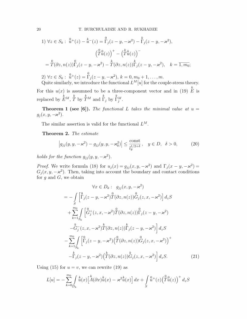
where j = 1, 2 is a fixed number, y an arbitrary fixed point in Dk, k = 0,m0.Functional (18) is defined in the class of regular vector functions in Dk (k =0,m0) satisfying the conditions:
20 T. BURCHULADZE AND R. RUKHADZE
1) ∀z ∈ Sk : 0u+(z)− ku−(z) =0Γj(z − y,−κ2)−
kΓj(z − y,−κ2),
( 0T 0u(z)
)+−
( kT ku(z)
)−
=0T (∂z, n(z))
0Γj(z − y,−κ2)−
kT (∂z, n(z))
kΓj(z − y,−κ2), k = 1,m0;
2) ∀z ∈ Sk : 0u+(z) =0Γj(z − y,−κ2), k = 0,m0 + 1, . . . , m.
Quite similarly, we introduce the functional LM [u] for the couple-stress theory.
For this u(x) is assumned to be a three-component vector and in (19)kE is
replaced bykEM ,
kT by
kTM and
kΓj by
kΓM
j .
Theorem 1 (see [6]). The functional L takes the minimal value at u =gj(x, y,−κ2).
The similar assertion is valid for the functional LM .
Theorem 2. The estimate∣
∣
∣gjj(y, y,−κ2)− gjj(y, y,−κ20)
∣
∣
∣ ≤ const
l1/2+δy
, y ∈ D, δ > 0, (20)
holds for the function gjj(y, y,−κ2).
Proof. We write formula (18) for uj(x) = gjj(x, y,−κ2) and Γj(x − y,−κ2) =Gj(x, y,−κ2). Then, taking into account the boundary and contact conditionsfor g and G, we obtain
The vectorkΓj(x − y,−κ2) defined by (8) belongs to the definition domain
of the functional L and, since gj(x, y,−κ2) imparts the minimal value to the
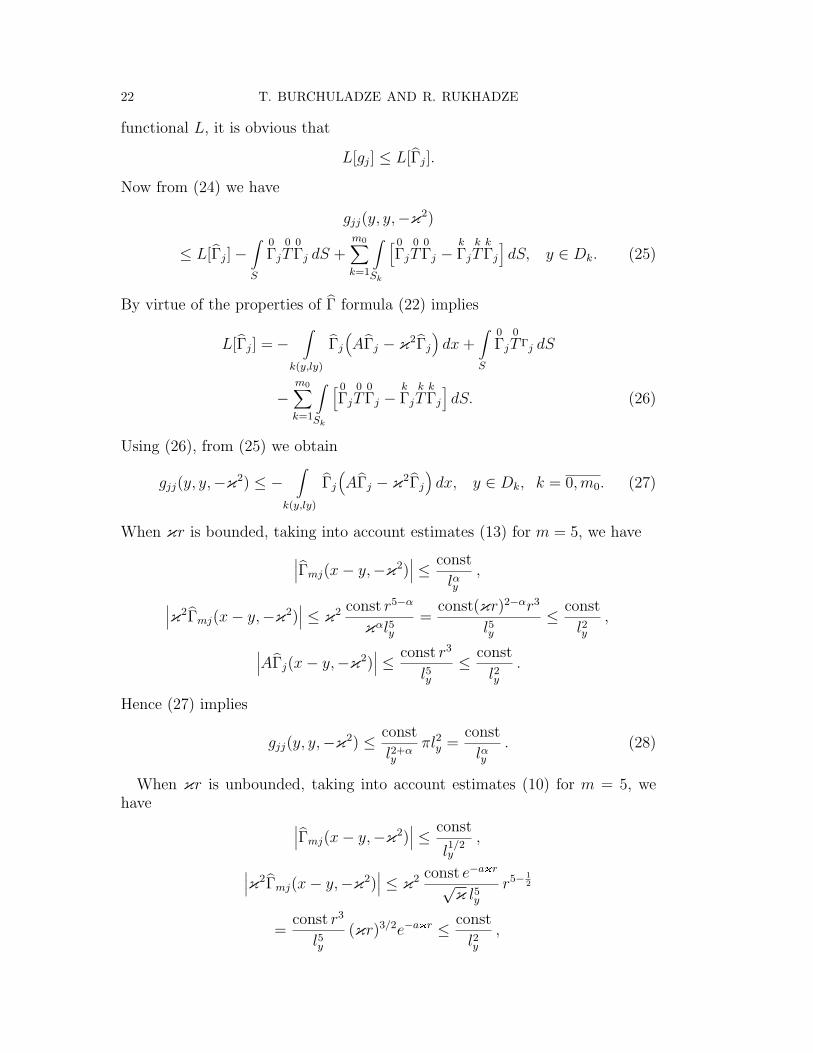
22 T. BURCHULADZE AND R. RUKHADZE
functional L, it is obvious that
L[gj] ≤ L[Γj].
Now from (24) we have
gjj(y, y,−κ2)
≤ L[Γj]−∫
S
0Γj
0T
0Γj dS +
m0∑
k=1
∫
Sk
[ 0Γj
0T
0Γj −
kΓj
kT
kΓj
]
dS, y ∈ Dk. (25)
By virtue of the properties of Γ formula (22) implies
L[Γj] =−∫
k(y,ly)
Γj
(
AΓj − κ2Γj
)
dx +∫
S
0Γj
0T Γj dS
−m0∑
k=1
∫
Sk
[ 0Γj
0T
0Γj −
kΓj
kT
kΓj
]
dS. (26)
Using (26), from (25) we obtain
gjj(y, y,−κ2) ≤ −∫
k(y,ly)
Γj
(
AΓj − κ2Γj
)
dx, y ∈ Dk, k = 0,m0. (27)
When κr is bounded, taking into account estimates (13) for m = 5, we have∣
∣
∣
Γmj(x− y,−κ2)∣
∣
∣ ≤ constlαy
,
∣
∣
∣κ2Γmj(x− y,−κ2)
∣
∣
∣ ≤ κ2 const r5−α
καl5y=
const(κr)2−αr3
l5y≤ const
l2y,
∣
∣
∣AΓj(x− y,−κ2)∣
∣
∣ ≤ const r3
l5y≤ const
l2y.
Hence (27) implies
gjj(y, y,−κ2) ≤ constl2+αy
πl2y =const
lαy. (28)
When κr is unbounded, taking into account estimates (10) for m = 5, wehave
∣
∣
∣
Γmj(x− y,−κ2)∣
∣
∣ ≤ const
l1/2y
,
∣
∣
∣κ2Γmj(x− y,−κ2)
∣
∣
∣ ≤ κ2 const e−a{r
√κ l5y
r5− 12
=const r3
l5y(κr)3/2e−a{r ≤ const
l2y,
ASYMPTOTIC DISTRIBUTION OF EIGENELEMENTS 23
∣
∣
∣AΓj(x− y,−κ2)∣
∣
∣ ≤ constκ2r−a{r
√κl5y
r5− 12 ≤ const
l2y.
Hence (27) implies
gjj(y, y,−κ2) ≤ const
l5/2y
πl2y =const
l1/2y
.
We assume that α = 12 in (28).
Let us estimate gjj(y, y,−κ2) from below. For this we introduce the followingnotation:
M [u] =m0∑
k=0
∫
Dk
[ kE(ku, ku) + κ2 ku2
]
dx,
M0[u] =m0∑
k=0
∫
Dk
[ kE(ku, ku) + κ2
0ku2
]
dx,
N [u] =m0∑
k=1
∫
Sk
[
0u+(z)0T (∂z, n(z))
0Γj(z − y,−κ2)
− ku−(z)kT (∂z, n(z))
kΓj(z − y,−κ2)
]
dzS.
Then L[u] = M [u]− 2N [u] and, since κ20 ≤ κ2, we have M0[u] ≤ M [u]. Now
L[
gj(x, y,−κ2)]
= min L[u] = min(
M [u]− 2N [u])
≥≥ min(
M0[u]− 2N [u])
.
Let the vector function ϕ(x, y) impart a minimal value to the functionalP [u] = M0[u] − 2N [u]. Then ϕ(x, y) belongs to the definition domain of thefunctional L and is a regular in the domain Dk (k = 0,m0) solution of theequation
∀x ∈ Dk : A(∂x)ϕ(x, y)− κ20ϕ(x, y) = 0, k = 0,m0.
After writing formula (18) for ϕ(x, y), where Γ = G, we obtain
∀(x, y) ∈ Dk ×Dk : ϕ(x, y) = −∫
S
0Γj(z − x,−κ2)
0T
0Gj(z, y,−κ2
0) dzS
+m0∑
k=1
∫
Sk
[ 0Gj(z, x,−κ2)
0T
0Γj(z − y,−κ2)
−kG−
j (z, x,−κ20)
kT
kΓj(z − y,−κ2)
]
dzS
−m0∑
k=1
∫
Sk
[ 0Γj(z, x,−κ2)
( 0T
0Gj(z, y,−κ2
0))
−kΓj(z − x,−κ2)
( kT
kGj(z, y,−κ2
0))−
]
dzS,
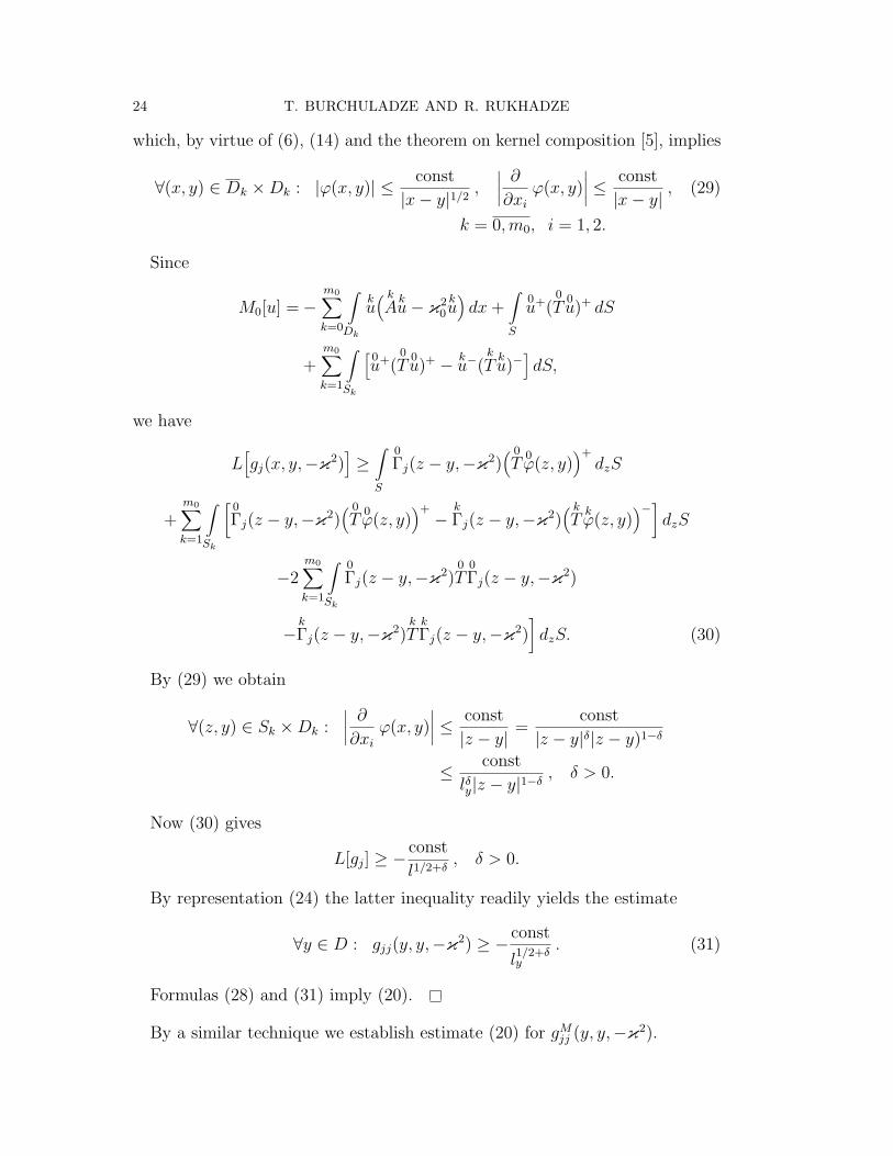
24 T. BURCHULADZE AND R. RUKHADZE
which, by virtue of (6), (14) and the theorem on kernel composition [5], implies
∀(x, y) ∈ Dk ×Dk : |ϕ(x, y)| ≤ const|x− y|1/2 ,
∣
∣
∣
∣
∂∂xi
ϕ(x, y)∣
∣
∣
∣
≤ const|x− y|
, (29)
k = 0,m0, i = 1, 2.
Since
M0[u] =−m0∑
k=0
∫
Dk
ku( kAku− κ2
0ku)
dx +∫
S
0u+(0T 0u)+ dS
+m0∑
k=1
∫
Sk
[0u+(0T 0u)+ − ku−(
kT ku)−
]
dS,
we have
L[
gj(x, y,−κ2)]
≥∫
S
0Γj(z − y,−κ2)
( 0T 0ϕ(z, y)
)+dzS
+m0∑
k=1
∫
Sk
[ 0Γj(z − y,−κ2)
( 0T 0ϕ(z, y)
)+−
kΓj(z − y,−κ2)
( kT kϕ(z, y)
)−]
dzS
−2m0∑
k=1
∫
Sk
0Γj(z − y,−κ2)
0T
0Γj(z − y,−κ2)
−kΓj(z − y,−κ2)
kT
kΓj(z − y,−κ2)
]
dzS. (30)
By (29) we obtain
∀(z, y) ∈ Sk ×Dk :∣
∣
∣
∣
∂∂xi
ϕ(x, y)∣
∣
∣
∣
≤ const|z − y|
=const
|z − y|δ|z − y)1−δ
≤ constlδy|z − y|1−δ , δ > 0.
Now (30) gives
L[gj] ≥ − constl1/2+δ , δ > 0.
By representation (24) the latter inequality readily yields the estimate
∀y ∈ D : gjj(y, y,−κ2) ≥ − const
l1/2+δy
. (31)
Formulas (28) and (31) imply (20).
By a similar technique we establish estimate (20) for gMjj (y, y,−κ2).
ASYMPTOTIC DISTRIBUTION OF EIGENELEMENTS 25
8. Let us consider the first boundary-contact problem with eigenvalues: Find,in Dk (k = 0, m0), a regular vector w(x) = kw(x) = ( kw1,
kw2) which is a nontrivialsolution of the equations
∀x ∈ Dk :k˜A(∂x) kw(x) + γ kw(x) = 0, k = 0,m0,
and satisfies the contact conditions
∀z ∈ Sk : 0w+(z) = kw−(z),( 0T 0w(z)
)+=
( kT kw(z)
)−, k = 1,m0,
and the boundary condition
∀z ∈ Sk : 0w+(z) = 0, k = 0,m0 + 1, . . . , m.
We denote this problem bycIγ . If in problem
cIγ we replace ˜A by ˜M , T by TM
and assume w(x) to be a three-component vector, then the resulting problem
with eigenvalues is denoted bycIM
γ .
It can be shown by the known technique [4] that problemcIγ is equivalent to
a system of integral equations
w(x) = (γ + κ20)
∫
D
˜G(x, y,−κ20)w(y) dy, (32)
where ˜G =1rG
1r, and problem
cIM
γ is equivalent to a system of integral equations
w(x) = (γ + κ20)
∫
D
˜GM(x, y,−κ20)w(y) dy, (33)
where ˜GM =2rGM
2r. By virtue of (13) and (14) equations (32) and (33) are
integral equations with a symmetric kernel of the class L2(D). Hence it fol-lows that there exists a countable system of eigenvalues (γn + κ2
0)∞n=1 and
the corresponding (orthonormal in D) system of eigenvectors (w(n)(x))∞n=1 =( kw(n)(x))∞n=1, x ∈ Dk, k = 0,m0, of equation (32). This in turn implies that
(γn)∞n=1 and (w(n)(x))∞n=1 are the eigenvalues and eigenvectors of problemcIγ . It
has been established [1] that all γn > 0. Moreover, in [7] it is proved that thesystem (w(n)(x))∞n=1 forms a complete system in L2(D). By the properties of avolume potential we conclude that the eigenvectors are regular. What has beensaid above can be repeated for the eigenvalues and eigenvectors of problem
cIM
γ .
9. In deriving asymptotic formulas, the Tauber type theorem due to Ikehara[8], [9] plays a decisive role. Let us formulate this theorem for series [9].
Theorem 3. Let λn be an increasing sequence of real numbers,
F (z) =∞∑
n=1
an
λzn
, Re(z) > 1,
26 T. BURCHULADZE AND R. RUKHADZE
where an ≥ 0, n = 1, 2, . . . , and assume that F (z) can be analytically continuedonto the straight line Re(z) = 1 and has no singularities at the points of thisstraight line except for the point z = 1 at which it has a first order pole with theprincipal part A
z−1 . Thenn
∑
k=1
ak ∼ Aλn.
By expanding the kernel in eigenfunctions we obtain
˜G(x, y,−κ2)− ˜G(x, y,−κ20) = (κ2
0 − κ2)∞∑
n=1
w(n)(x)× w(n)(y)(γn + κ2)(γn + κ2
0), (34)
where x, y ∈ Dk, k = 0,m0, and the symbol × denotes the matrix product of acolumn vector by a row vector (the dyad product)
w(n)(x)× w(n)(y) =∥
∥
∥w(n)i (x)w(n)
k (x)∥
∥
∥
i,k=1,2.
After passing in equality (34) to the limit as x → y, we obtain
(κ20 − κ2)
∞∑
n=1
[w(n)j (y)]2
(γn + κ2)(γn + κ20)
= limx→y
[1rΓjj(x− y,−κ2)
1r −
1rΓjj(x− y,−κ2
0)1r]
− limx→y
[1rgjj(x, y,−κ2)
1r −
1rgjj(x, y,−κ2
0)1r]
, (35)
x, y ∈ Dk, k = 0,m0, j = 1, 2.
Denote
hj(y,κ) =1rgjj(y, y,−κ2
0)1r −
1rgjj(y, y,−κ2)
1r
= ρ[
gjj(y, y,−κ20)− gjj(y, y,−κ2)
]
.
By (20) hj(κ) = O(1) as κ →∞. Using (11), we have
limx→y
[1rΓjj(x− y,−κ2)
1r −
1rΓjj(x− y,−κ2
0)1r]
= limx→y
ρk
[ kΓjj(x− y,−κ2)−
kΓjj(x− y,−κ2
0)]
= −An lnκκ0
, (36)
whereAk =
ρk
4π
( 1λk + 2µk
+1µk
)
, k = 0,m0.
Let λ = κ20 −κ2, γn = γn +κ2
0 . Let us choose κ0 such that γ1 +κ20 = γ1 > 0.
Now by virtue of (36) it follows from (35) that
R(y, λ) = λ∞∑
n=1
[w(n)j (y)]2
γn(γn − λ), (37)
ASYMPTOTIC DISTRIBUTION OF EIGENELEMENTS 27
where
R(y, λ) = −Ak lnκκ0
+ hj(y, λ) = −Ak ln
√
1− λκ2
0+ hj(y, λ)
= −Ak ln√−λ− Ak ln
√
1κ2
0− 1
λ+ hj(y, λ)
= −Ak
√−λ + O(1) for λ → −∞, y ∈ Dk, k = 0,m0, j = 1, 2.
Divide both parts of (37) by 2πiλz and integrate from ε−i∞ to ε+i∞, where0 < ε < γ1 (z is a complex-valued parameter whose real part is sufficientlylarge). Applying the basic residue theorem, we obtain
12πi
ε+i∞∫
ε−i∞
λ dλγn(γn − λ)λz =
1γ z
n. (38)
Due to (38) we can rewrite (37) as
∞∑
n=1
[w(n)j (y)]2
γ zn
=1
2πi
ε+i∞∫
ε−i∞
R(y, λ)λz dλ. (39)
We perform the Carleman transformation [10] of the integral in the right-handpart of (39). The function R(y, λ)λ−z is analytic on the entire plane except forthe points 0, γ1, γ2, . . . and, by the Cauchy theorem, the integral of this functiontaken over the closed contour not containing these points internally, is equal tozero. By the Cauchy theorem the integral in the right-hand part of (39) can bewritten as
ε+i∞∫
ε−i∞
R(y, λ)λz dλ =
∫
L1
R(y, λ)λz dλ +
∫
C
R(y, λ)λz dλ +
∫
L2
R(y, λ)λz dλ, (40)
where L1 = (−∞− 0i,−ε− 0i), L2(−ε + 0i,−∞+ 0i), C is the circumference|λ| = ε. Clearly, λ = |λ|e−iπ on L1, λ = |λ|eiπ on L2, and λ = εeiθ on C. Wehave
∫
C
R(y, λ)λz dλ = iε1−z
π∫
−π
R(y, εeiθ)ei(1−z)θ dθ,
∫
L1
R(y, λ)λz dλ=eiπz
∞∫
ε
R(y,−λ)λz dλ,
∫
L2
R(y, λ)λz dλ=−e−iπz
∞∫
ε
R(y,−λ)λz dλ.
Hence by virtue of (39) and (40)
∞∑
n=1
[w(n)j (y)]2
γ zn
28 T. BURCHULADZE AND R. RUKHADZE
=ε1−z
2π
π∫
−π
R(y, εeiθ)ei(1−z)θ dθ +sin πz
π
∞∫
ε
R(y,−λ)λz dλ. (41)
Integrating by parts we obtain
∞∫
ε
ln√
λλz dλ =
ε1−z ln ε2(z − 1)
+ε1−z
2(z − 1)2 . (42)
By virtue of (42) we can rewrite (41) as
∞∑
n=1
[w(n)j (y)]2
γ zn
=ε1−z
2π
π∫
−π
R(y, εeiθ)ei(1−z)θ dθ
−sin π(z − 1)π
[
− Ak ln ε ε1−z
2(z − 1)− Akε1−z
2(z − 1)2 +∞∫
ε
O(1)λz dλ
]
. (43)
Due to Ikehara’s Theorem 3, (43) gives
n∑
p=1
[
w(p)j (y)
]2∼ Ak
2γn, j = 1, 2,
or, finally,
n∑
p=1
[
w(p)(y)]2∼ ρk
4π
( 1λk + 2µk
+1µk
)
γn, y ∈ Dk, k = 0,m0. (44)
On repeating the above reasoning, we obtain asymptotic formulas for eigen-vectors of problem
cIM
γ . Note only that in this case the eigenvectors (w(n)(x))∞n=1are three-component and, as follows from (12),
limx→y
[2rjj
kΓM
jj (x− y,−κ2)2rjj −
2rjj
kΓM
jj (x− y,−κ20)
2rjj
]
=ρk
4π
( 1λk + 2µk
+1
µk + αk
)
lnκ0
κ , j = 1, 2,
limx→y
[2r33
kΓM
33(x− y,−κ2)2r33 −
2r33
kΓM
33(x− y,−κ20)
2r33
]
=Ik
2π1
νk + βklnκ0
κ .
Therefore in the couple-stress elasticity
n∑
p=1
[
w(p)j (y)
]2∼ ρk
8π
( 1λk + 2µk
+1
µk + αk
)
γn, j = 1, 2, (45)
n∑
p=1
[
w(p)3 (y)
]2∼ Ik
4π1
νk + βkγn, y ∈ Dk, k = 0,m0. (46)
ASYMPTOTIC DISTRIBUTION OF EIGENELEMENTS 29
10. From (35) we obtain
−R(y,κ)κ2 − κ2
0=
∞∑
n=1
[w(n)(y)]2
(γn + κ20)(γn + κ2
0)≤
∞∑
n=1
[w(n)(y)]2
(γn + κ20)2 . (47)
Applying the Bessel inequality, we have
∞∑
n=1
[w(n)(x)]2
(γn + κ20)2 ≤
∫
D
∣
∣
∣
˜G(x, y,−κ20)
∣
∣
∣
2dy, x ∈ Dk,
which, taking into account estimates (14), implies the existence and uniformboundedness of the sum of the series
If we integrate (47) in the domain D, then, recalling that the vectors(w(n)(x))∞n=1 are orthonormal in D, we obtain
−∫
D
R(y,κ) dy = (κ2 − κ20)
∞∑
n=1
1(γn + κ2)(γn + κ2
0),
−∫
D
R(y,κ) dy =∫
D
2Ak lnκκ0
dy −∫
D
hj(y,κ) dy
= 2 lnκκ0
m0∑
k=0
Ak mes Dk −∫
D
hj(y,κ) dy. (49)
Denote by (Dk)η that part of Dk (k = 0,m0) where the distance from thepoints to the boundary of Dk is less than η; Dη =
m0∪k=0
(Dk)η. Now,
∫
D
hj(y,κ) dy =∫
D\Dη
hj(y,κ) dy +∫
Dη
R(y,κ) dy +∫
Dη
2Ak lnκκ0
dy, (50)
∫
Dη
2Ak lnκκ0
dy = 2 lnκκ0
m0∑
k=0
Ak mes(Dk)η = 2 lnκκ0
m0∑
k=0
AkO(η), (51)
∫
Dη
R(y,κ) dy ≤ const(κ2 − κ20) mes Dη = (κ2 − κ2
0)O(η), (52)
∫
D\Dη
hj(y,κ) dy = O(η12−δ). (53)
30 T. BURCHULADZE AND R. RUKHADZE
The validity of (51) is obvious. (52) holds by virtue of (48), while (53) byvirtue of (20). Let λ = κ2
0 − κ2, η = 1{2−{2
0= − 1
λ . Then (51), (52), (53) imply
∫
Dη
2Ak lnκκ0
dy =m0∑
k=0
Ak2(
ln√−λ + ln
√
1κ2
0− 1
λ
)
O(1
λ
)
, (54)
∫
Dη
R(y,κ) dy = λO(1
λ
)
= O(1), (55)
∫
D\Dη
hj(y,κ) dy = O( 1
λ12−δ
)
. (56)
On account of (54), (55), (56), from (50) we obtain∫
D
hj(y,κ) dy = 2 ln√−λ
m0∑
k=0
AkO(1
λ
)
+2 ln
√
1κ2
0− 1
λ
m0∑
k=0
AkO(1
λ
)
+ O(1) + O( 1
λ12−δ
)
. (57)
By virtue of (57), formula (49) gives
−∫
D
R(y,κ) dy = 2 ln√−λ
m0∑
k=0
Ak mes Dk
+2 ln
√
1κ2
0− 1
λ
m0∑
k=0
Ak mes Dk − 2 ln√−λ
m0∑
k=0
AkO(1
λ
)
−2 ln
√
1κ2
0− 1
λ
m0∑
k=0
AkO(1
λ
)
+ O(1) + O( 1
λ12−δ
)
= R∗(λ).
Hence (47) implies
R∗(λ) = λ∞∑
n=1
1γn(γn − λ)
. (58)
Divide both parts of (58) by 2πiλz and integrate from ε − i∞ to ε + i∞,where 0 < ε < γ1. Now in the same manner as above we have
∞∑
n=1
1γ z
n= −ε1−z
2π
π∫
−π
R∗(εeiθ)ei(1−z)θ dθ
−sin π(z − 1)π
[
−
m0∑
k=0Ak mes Dk ln ε ε1−z
z − 1−
m0∑
k=0Ak mes Dkε1−z
(z − 1)2
+∞∫
ε
O(1)λz dλ + const
ln ε ε−z
z+ const
e−z
z2 + constε
12+δ−z
12 + δ − z
]
. (59)
ASYMPTOTIC DISTRIBUTION OF EIGENELEMENTS 31
Applying Ikehara’s theorem, from (59) we obtain
limn→∞
nγn
=m0∑
k=0
Ak mes Dk
or, finally,
limn→∞
nγn
=14π
m0∑
k=0
ρk
( 1λk + 2µk
+1µk
)
mes Dk. (60)
If (γn)∞n=1 are the eigenvalues of problemcIM
γ , then, as above, we obtain
limn→∞
nγn
=14π
m0∑
k=0
[
ρk
( 1λk + 2µk
+1
µk + αk
)
+Ik
νk + βk
]
mes Dk. (61)
To conclude, the results of this paper can be formulated as
Theorem 4. The asymptotic distribution of eigenelements of the basic two-dimensional boundary-contact problems of oscillation is given by formulas (44)and (60) in the classical theory of elasticity, and by formulas (45), (46) and (61)in the couple-stress theory of elasticity.
References
1. V. Nowacki, The theory of elasticity. (Translated from Polish into Russian)Mir, Moscow, 1975.
2. O. I. Maisaya, Investigation of the basic boundary value problems ofthe plane couple-stress theory of elasticity. (Russain) Tbilisi University Press,Tbilisi, 1974.
3. B. G. Korenev, Introduction to the theory of Bessel functions. (Russian)Nauka, Moscow, 1971.
4. M. O. Basheleishvili, On the solution of piecewise-inhomogeneous aniso-tropic elastic media by the method of Fredholm integral equations. (Russian)Trudy Gruzin. Politekh. Inst., 1965, No. 2(100), 3–11.
5. D. G. Natroshvili, Estimates of Green tensors of the elasticity theory andsome of their applications. (Russian) Tbilisi University Press, Tbilisi, 1978.
6. T. Burchuladze and R. Rukhadze, Asymptotic distribution of eigenfunc-tions and eigenvalues of the basic boundary-contact oscillation problems of theclassical theory of elasticity. Georgian Math. J. 6(1999), No. 2, 107–126.
7. T. Burchuladze and R. Rukhadze, Fourier method in three-dimensionalboundary-contact dynamic problems of elasticity. Georgian Math. J. 2 (1995),No. 6, 559–576.
8. S. Ikehara, An extension of Landau’s theorem in the analytic theory ofnumbers. J. Math. Phys. M.I.T. 10(1931), 1–12.
32 T. BURCHULADZE AND R. RUKHADZE
9. N. Wiener, The Fourier integral and certain of its applications. (Translatedinto Russian) Gosud. Izd. Fiz.-Mat. Lit., Moscow, 1963; English original:Cambridge University Press, 1933.
10. T. Carleman, Proprietes asymptotiques des fonctions fondamentals desmembran vibrantes. Comptes Rendus des Mathematiciens Scandinaves a Stock-holm, 1934, Stockholm, 34–44; see also in T. Carleman, Collected works, 471–483, Malmo, 1960.
(Received 16.06.1998)
Authors’ addresses:
T. BurchuladzeA. Razmadze Mathematical InstituteGeorgian Academy of Sciences1, M. Aleksidze St., Tbilisi 380093GeorgiaE-mail: [email protected]
R. RukhadzeGeorgian Technical UniversityDepartment of Mathematics (3)77, M. Kostava St., Tbilisi 380075Georgia


![Asymptotic behavior of singularly perturbed control …€¦ · Asymptotic behavior of singularly perturbed control ... [Lions, Papanicolau, Varadhan 1986]; ... Asymptotic behavior](https://static.documents.pub/doc/80x56/5b7c19bc7f8b9a9d078b9b98/asymptotic-behavior-of-singularly-perturbed-control-asymptotic-behavior-of-singularly.jpg)


