rspa.royalsocietypublishing.org Research Cite this article: Shaw AD, Champneys AR, Friswell MI. 2016 Asynchronous partial contact motion due to internal resonance in multiple degree-of-freedom rotordynamics. Proc. R. Soc. A 472: 20160303. http://dx.doi.org/10.1098/rspa.2016.0303 Received: 3 May 2016 Accepted: 1 August 2016 Subject Areas: mechanical engineering, applied mathematics Keywords: rotating machines, internal resonance, whirl, stator contact, bifurcation Author for correspondence: A. D. Shaw e-mail: [email protected]Asynchronous partial contact motion due to internal resonance in multiple degree-of-freedom rotordynamics A. D. Shaw 1 , A. R. Champneys 2 and M. I. Friswell 1 1 College of Engineering, Swansea University, Bay Campus, Fabian Way, Swansea SA1 8EN, UK 2 Department of Engineering Mathematics, University of Bristol, Merchant Venturers Building, Woodland Road, Clifton BS8 1UB, UK ADS, 0000-0002-7521-827X Sudden onset of violent chattering or whirling rotor– stator contact motion in rotational machines can cause significant damage in many industrial applications. It is shown that internal resonance can lead to the onset of bouncing-type partial contact motion away from primary resonances. These partial contact limit cycles can involve any two modes of an arbitrarily high degree-of-freedom system, and can be seen as an extension of a synchronization condition previously reported for a single disc system. The synchronization formula predicts multiple drivespeeds, corresponding to different forms of mode-locked bouncing orbits. These results are backed up by a brute-force bifurcation analysis which reveals numerical existence of the corresponding family of bouncing orbits at supercritical drivespeeds, provided the damping is sufficiently low. The numerics reveal many overlapping families of solutions, which leads to significant multi-stability of the response at given drive speeds. Further, secondary bifurcations can also occur within each family, altering the nature of the response and ultimately leading to chaos. It is illustrated how stiffness and damping of the stator have a large effect on the number and nature of the partial contact solutions, illustrating the extreme sensitivity that would be observed in practice. 2016 The Authors. Published by the Royal Society under the terms of the Creative Commons Attribution License http://creativecommons.org/licenses/ by/4.0/, which permits unrestricted use, provided the original author and source are credited. on June 10, 2018 http://rspa.royalsocietypublishing.org/ Downloaded from
Transcript
rspa.royalsocietypublishing.org
ResearchCite this article: Shaw AD, Champneys AR,Friswell MI. 2016 Asynchronous partial contactmotion due to internal resonance in multipledegree-of-freedom rotordynamics. Proc. R.Soc. A 472: 20160303.http://dx.doi.org/10.1098/rspa.2016.0303
Asynchronous partial contactmotion due to internalresonance in multipledegree-of-freedomrotordynamicsA. D. Shaw1, A. R. Champneys2 and M. I. Friswell1
1College of Engineering, Swansea University, Bay Campus,Fabian Way, Swansea SA1 8EN, UK2Department of Engineering Mathematics, University of Bristol,Merchant Venturers Building, Woodland Road, Clifton BS8 1UB, UK
ADS, 0000-0002-7521-827X
Sudden onset of violent chattering or whirling rotor–stator contact motion in rotational machines can causesignificant damage in many industrial applications.It is shown that internal resonance can lead to theonset of bouncing-type partial contact motion awayfrom primary resonances. These partial contact limitcycles can involve any two modes of an arbitrarilyhigh degree-of-freedom system, and can be seen as anextension of a synchronization condition previouslyreported for a single disc system. The synchronizationformula predicts multiple drivespeeds, correspondingto different forms of mode-locked bouncing orbits.These results are backed up by a brute-forcebifurcation analysis which reveals numerical existenceof the corresponding family of bouncing orbitsat supercritical drivespeeds, provided the dampingis sufficiently low. The numerics reveal manyoverlapping families of solutions, which leads tosignificant multi-stability of the response at givendrive speeds. Further, secondary bifurcations canalso occur within each family, altering the nature ofthe response and ultimately leading to chaos. It isillustrated how stiffness and damping of the statorhave a large effect on the number and nature ofthe partial contact solutions, illustrating the extremesensitivity that would be observed in practice.
2016 The Authors. Published by the Royal Society under the terms of theCreative Commons Attribution License http://creativecommons.org/licenses/by/4.0/, which permits unrestricted use, provided the original author andsource are credited.
on June 10, 2018http://rspa.royalsocietypublishing.org/Downloaded from
1. IntroductionThe lateral vibrations of rotating machinery are an important issue in many engineeredsystems [1,2]. Understanding of rotating machinery in linear operating regimes is wellestablished, with classical methods from linear algebra being applied to deduce the whirlspeeds of rotational systems with any number of degrees of freedom. However, there are manyoutstanding problems concerning nonlinearity in rotating systems, and these are leading to newapproaches in a variety of industrial applications. One novelty compared with non-rotatingvibration problems is that matrices associated with rotordynamic systems are highly non-normaldue to the presence of gyroscopic forces. The interplay between the non-normality and nonlineareffects can lead to counterintuitive dynamical consequences (e.g. [3,4]).
By their nature, rotors are susceptible to geometric nonlinearity [5,6] and can experiencepotentially catastrophic effects from a nonlinear viscous phenomenon known as oil whip [7–9].Patel & Darpe [10] noted that cracks in rotors also induce nonlinear effects and explored theseeffects with bifurcation analysis. Other forms of nonlinearity can arise through squeeze-filmdamping effects [11] or through additional automatic dynamic balancer mechanisms [4,12,13].However, the focus for the current work is nonlinearity due to the rotor making contact with anexternal stator.
Rotor–stator contact is an issue that affects a wide variety of applications, fromturbomachinery [14] to drilling for mineral extraction [15] and is driving a large body ofresearch [16]. Many rotating devices incorporate magnetic bearing systems [17,18], and thesemust be designed with consideration of the consequences of a touch-down event in response to afailure or disturbance [19]. Ehrich [20] has compiled examples of numerous contact phenomenawitnessed in tests on turbomachinery, including period-doubling bifurcation routes to chaos,subharmonic resonance and other surprising effects such as bearing phenomenon that lead toa rotor slowly ‘switching’ between two amplitudes of vibration.
Contact nonlinearities are typically due to friction during contact and discontinuous stiffnesseffects, and the typical response behaviours are classified by Jacquet-Richardet et al. within threeclassifications; forward whirl annular motion, backward whirl motion and rebounds [14]. Forward whirlannular motion occurs synchronously; the shaft whirls in constant contact with the stator, at thesame angular speed and direction as the shaft rotation. This generates heat on the contacting sideof the shaft, and this results in a bending known as the Newkirk effect [1,21]. Backward whirlmotion again occurs with constant contact between rotor and stator, but in these cases the frictionis sufficient to cause the shaft to whirl in the opposite direction to the shaft rotation. In many cases,there is zero relative sliding between the two surfaces, in which case the whirling is typically veryrapid, known as dry whirl or dry whip. Owing to its potentially destructive nature, the stabilityand onset of the dry whirl condition has been widely studied (e.g. [22–25]). In addition, if torsionaldeformation of the shaft is considered, constant contact response may also include a componentof torsional vibration [26], perhaps including complex stick-slip phenomena [27–30].
Rebound motion consists of intermittent contact between rotor and stator, and while manynames for forms of this motion are used in the literature (chatter, intermittent contact, rattle,bouncing), we will henceforth refer to these responses as exhibiting partial contact. Some of theearliest work on partial contact motion was summarized in the review by Ehrich [20]. Hallmarksof such motion can be seen in the observation of sum and difference combination resonancesin the response of impacting rotors [31], and a case where a non-rigid stator was shown towhirl [32]. Neilson & Barr [33] constructed an experimental rig for rotor–stator contact, andshowed that the resulting spectral output had synchronous content (i.e. at integer ratios to thedrive speed frequency) as well as asynchronous sidebands. During the 1980s, researchers beganto view these systems through the framework of nonlinear dynamical systems theory [34,35]and later numerical and experimental studies began to show evidence of period doublingphenomena and chaos. For example, Muzsynska & Goldman [36] numerically demonstratedbifurcations to period-n motion and transitions to chaos under variation of shaft speed, withgood qualitative comparison to experimental results. Chu & Zhang [37] used Floquet analysis of
on June 10, 2018http://rspa.royalsocietypublishing.org/Downloaded from
orbits of a contacting Jeffcott rotor to trace the progression to chaos; their results bore similarity tothose of Muzsynska & Goldman [36], where brief regions of chaos were interspersed betweenwider regions of simpler period-n response. Edwards et al. [38] produced a numerical studyof a single contacting disc on a shaft that showed chaotic responses at every integer and half-integer multiples of the first critical drive speed, and demonstrated that this behaviour could besignificantly influenced by torsional effects.
In other work, Karpenko et al. [39] developed a piecewise smooth model for rotorsexperiencing frictionless impacts with a snubber ring, and in later work examined the responsespace of this system with bifurcation analysis, and revealed the basins of attraction for varioussolutions [40]. Pavlovskaia considered a similar system, but where the snubber ring springs werepreloaded to create additional nonlinearity [41], and Karpenko et al. [42] went on to comparethese predictions with experiment, where the experimental stator could rotate on a bearingto approximate the assumption of zero friction contact. Chu & Lu [43] studied a two- discexperimental system, showing some highly complex multi-period and quasi-periodic behaviour,although the authors comment that they could not directly trace the route into chaos due toexperimental control issues. Further experimental data have been provided by Torkhani et al. [44]on a two disc experimental rig, which also demonstrated agreement with a numerical model.
Some researchers have employed harmonic balance methods to investigate these systems,instead of the piecewise-smooth methodology used in some of the works above. For example,Kim & Noah [45] found solutions using a method that combined harmonic balance with analternating frequency time-domain analysis, that assumed two fundamental frequencies, tohandle the observed effect that some response frequencies were not periodic in the drive speedfrequency. Von Groll & Ewins [46] performed a harmonic balance method on a system where thestator had inertia as well as stiffness, which found both constant contact solutions but also somepartial contact solutions. While this method was inefficient when initially locating such solutions,it was augmented with arc-length continuation to trace families of solutions once a solution hadbeen found.
Cole & Keogh [47] emphasize the distinction between two forms of partial contact motion:synchronous partial that occurs at harmonics and subharmonics of the rotor shaft speed, andasynchronous partial contact where the frequency of impacts is apparently unrelated to the shaftspeed. This work suggests that synchronous partial contact occurs when the rotor/stator systemcannot be assumed to be axisymmetric, and this appears to be supported within the literaturecited above. Solutions for asynchronous partial contact orbits are harder to solve, because thefundamental frequency of the asynchronous must be found in addition to the Fourier seriescomponents. In [47], this frequency is found by balancing the energy immediately before andafter an impact accounting for the coefficient of restitution; hence relying on the assumption ofinstantaneous contact. The same authors use a similar assumption to solve synchronous responsesin [48]. It is interesting to note the recent work of Mora et al. [49] who use recent techniques frompiecewise-smooth dynamical systems theory to analyse the bifurcations that can occur at suchimpacts at primary resonances.
An intriguing new insight into asynchronous partial contact motion was demonstrated in therecent paper by Zilli et al. [50]. Here they find a condition for isolated bouncing motion that cancoexist with the fundamental response curve, away from any primary resonances. They explainedthe onset of this motion through a synchronization condition between the forward and backwardwhirling modes of this system that made it susceptible to asynchronous partial contact motion.This led to an approximate prediction of the drive speeds that could cause this motion. In [51], thepresent authors reported a generalization of Zilli’s work to apply to any two modes of a two discsystem, with any combination of forward and backward whirling. This showed further forms ofasynchronous response, made possible by the increased number of linear whirling modes of themulti disc system. This condition is reproduced in §2 below and is argued here for the first timeto be identifiable as form of internal resonance.
The main focus of the present work is to perform an in-depth brute-force numerical bifurcationanalysis of a typical multiple degree-of-freedom rotating machine, with rotor stator contact.
on June 10, 2018http://rspa.royalsocietypublishing.org/Downloaded from
We find in many cases that multiple forms of asynchronous partial contact motion can occurat a single drive speed. We show how these can be related to underlying whirling modes of thesystem by the internal resonance condition. The ultimate goal is to gain an understanding of theconditions under which partial contact cycles might be triggered, and hence to understand howto avoid these potentially damaging oscillations in practice.
The rest of the paper is outlined as follows. Section 2 contains an explanation of differentforms of vibration modes in a multiple degree-of-freedom rotating system and how these dependon drive speed. The internal resonance condition that predicts the onset of partial contact cyclesin the presence of a stator is then derived, with care taken to explain the assumptions underlyingthe calculation. Section 3 then presents the example system on which we perform numericalcomputations, as well as outlining the numerical method used. Section 4 contains the results of abrute-force bifurcation analysis, together with a discussion of the origin of the different forms ofpartial contact solutions obtained. The results are presented for both a system with low contactstiffness and a purely elastic stator which permits a rich variety of responses, and then for a casemore commonly encountered in practice, where the contacts have high stiffness and significantdamping. It is shown that the internal resonance condition explains the onset of bouncing motion,even as more complex orbits evolve. Finally, §5 draws conclusions and suggests avenues forfuture work.
2. Analytical considerationsThis section firstly presents a general mathematical description of the system under consideration,and how its motion may be described in terms of whirling modes of the underlying linearconservative system. It then shows how an internal resonance between these whirling modesis a necessary condition for asynchronous periodic contact.
(a) General description of the systemWe consider a general class of multiple degree-of-freedom systems that rotate about an shaft ata constant rotating speed Ω , subject to constant out-of-balance forces. We further suppose thatthe free rotor has light external damping, but can be subject to frictionless contact with a singleconcentric stator of fixed clearance, at a single point on the shaft. The shaft is assumed to betorsionally and axially rigid, hence these degrees of freedom are ignored in favour of purelylateral vibration modes. The shaft is assumed to have negligible internal damping, to avoidpotential instabilities [1] that are not the focus of this work. Furthermore, it is assumed that allrotor bearings are isotropic and the stator clearance is circular with the same centre as the shaft. Allelements of the system behave in a manner consistent with linear assumptions apart from possiblerotor–stator contact; therefore, this is an example of a system with a single, local nonlinearity.
The equations of motion of this system can be written using the standard assumptions ofLagrangian mechanics as
Mq +ΩGq + Kq + Cq + N(q, q) = Re (Ω2b0 eiΩt), (2.1)
where the vector q ∈ Rn contains generalized rotations and displacements in a stationary
coordinate frame. The matrices M, C and K are symmetric mass, damping and stiffness matricesrespectively, and G is a skew-symmetric matrix of gyroscopic coupling terms. The vector b0captures the distribution of out of balance forces which are written in complex form [1], andi = √−1. In addition, there is a nonlinear term N(q, q), representing the rotor–stator contact whichwe discuss later.
This system may also be considered in a coordinate frame rotating with angular speedΩ aboutthe shaft centre line. Hence a transformation exists between the two coordinate systems:
q = T(Ωt)q, (2.2)
on June 10, 2018http://rspa.royalsocietypublishing.org/Downloaded from
where T(Ωt) is a time-varying rotational transformation matrix, and q represents generalizeddisplacements in the rotating system. Under such a transformation, equation (2.1) may betransformed to the form
M ¨q +ΩG ˙q + Kq + C ˙q + Kcq + N(q, ˙q) = b0. (2.3)
The system matrices are assumed to be isotropic, i.e. invariant under axial rotation, hence Mand C remain unchanged between equations (2.1) and (2.3). However, substitution of equation(2.2) into equation (2.1) requires expansion of derivatives using the chain rule, which results inadditional terms which are incorporated into the rotational forms of the gyroscopic and stiffnessmatrices denoted G and K, respectively. The term Kcq contains forces that originate from thetransformation of the term Cq in equation (2.1); however, these are kept separate from Kq forconvenience when separating the conservative parts of the system from the non-conservativeparts. The matrix K is symmetric, the matrices G and Kc are skew symmetric. Note that allmatrices with a tilde are functions of shaft speedΩ . If it is assumed that the nonlinear force acts ina purely radial direction (as in frictionless contact) and is axisymmetric, the form of N(q, q) maybe used in either coordinate system unchanged. Also note that the out of balance forcing term,has now become a constant forcing term instead of a harmonic time varying term. Specific detailsof these matrices and transformations are given later on.
(b) Whirling modes of the underlying linear conservative systemIf forcing, damping and nonlinearity are neglected, a linear conservative system is extracted fromequation (2.3):
M ¨q +ΩG ˙q + Kq = 0. (2.4)
Owing to the first derivative term in equation (2.4), it is convenient to transform it into state spaceform prior to solution:
˙y = Ay, y ={
q˙q
}and A =
[0 I
M−1K ΩM−1G
]. (2.5)
Solutions to equation (2.5) have formy = wi esit,
where wi are the first-order eigenvectors and si are the eigenvalues which are purely imaginary.From the definition of y, the first-order eigenvectors must have form w = [vi, sivi]T, and, therefore,it is possible to extract the second-order eigenvectors that satisfy equation (2.4) directly with
q = vi esit.
If the number of degrees of freedom in equation (2.4) is n, there are 2n states in equation (2.5)and hence there are 2n eigenvalues and associated eigenvectors. The mode shapes are complexand appear in conjugate pairs, so that a motion based on a single conjugate pair of eigensolutionswill have form
q = Vivi esit + V∗i v∗
i es∗i t, (2.6)
where an asterisk indicates complex conjugation and Vi is a complex amplitude. Evaluatingequation (2.6) at any convenient point along the shaft will show a displacement that follows acircular path around the centre line, at an angular speed ωi, known as the whirl speed. If themotion is anticlockwise, the same direction as shaft speed Ω , the whirl speed ωi is defined aspositive and the motion is described as a forward whirl mode. Otherwise, the motion is describedas a backward whirl mode and ωi is negative. It may be shown that all eigenvalue pairs may beexpressed as
si, s∗i = ±iωi
and that all motions of the conservative system can be expressed as a superposition of multiplewhirl modes in the form of equation (2.6).
on June 10, 2018http://rspa.royalsocietypublishing.org/Downloaded from
A similar analysis could be performed starting with equation (2.1) instead of equation (2.3),hence deriving whirl modes in the stationary coordinate system. However, it can be seen from theform of the transformation between the two systems that whirl speeds in the stationary systemwill be related to those in the rotating system by
ωi = ωi +Ω (2.7)
and that the whirl mode shapes will be identical. This relationship allows the possibility thata forward whirl mode in the stationary system is a backward whirl in the rotating system, ifΩ >ωi. In the majority of rotordynamics literature, the greatest attention is paid to modes thatrepresent forward whirl in the stationary frame, as these are excited by the out of balance forcesand, therefore, determine linear critical rotation speeds. However, in this work all modes, eitherbackward or forward, are equally relevant because impacts with the stator can excite any mode.
(c) Internal resonance condition for asynchronous partial contact orbitsSection 2a established that the underlying linear system has responses in the forms of whirlingmotions, where the whirling speeds are functions of shaft speed Ω . These underlying modes willhave a strong effect on the system response unless the nonlinear and non-conservative elementsare strong, and therefore a partial contact motion must interact with these underlying modes tobe sustained. Two limits in which such an observation can be made precise are when the statornonlinearity is sufficiently weak, then a harmonic balance approximation can be made, as forexample in [46]. Alternatively, in the rigid stator limit, the condition for the linear undampedsystem to have a periodic solution can be considered as the conditions for a grazing bifurcation(e.g. [49]). Further discussion on this point will be made in §5.
A response that predominately consists of motion in a single mode will consist of a circularorbit in an appropriate frame and hence will not be able to reproduce the complexity of anasynchronous partial contact orbit. Therefore, an analysis proceeds by considering any twowhirling modes of the underlying linear system, with whirl speeds ωi and ωj in the rotating frame.
By definition, asynchronous partial contact is aperiodic with shaft speed Ω in the stationarycoordinate system. Therefore, we consider motion in the rotating frame, as this means that theout of balance force is now a constant term and, therefore, does not directly affect the problemof seeking the fundamental period for oscillation. If it is assumed that the whirling speeds are besimilar to those of the underlying linear conservative system, the condition for periodicity in therotating system is that a rational ratio exists between the linear rotation speeds. This conditioncan be stated as
(p − q)ωi = pωj, (2.8)
where p and q are integers. Substituting equation (2.7) into equation (2.8) enables us to rewritethis relationship in terms of the stationary-frame whirl speeds:
qΩ = p(ωj − ωi) + qωi. (2.9)
The reason for the slightly contrived form of equation (2.8) becomes clear when equation (2.9)is compared with the work of Zilli et al. [50]. That paper studied the simplest form of the systemdescribed in Section 2a, with just 2 d.f., representing single forward and backward whirl modes(in the stationary frame). Let us call these modes ωFW and ωBW, respectively. From a physicalargument based on the periodic synchronization of the two whirling modes and the out of balanceforcing phasor, a condition for partial contact orbits was given by Zilli et al. as
Ω = n(ωFW + ωBW) + ωFW, (2.10)
where the hats indicate the non-dimensional quantities used. Equation (2.10) is obviouslyidentical to (2.9) under the substitution q = 1, ωi = ωFW and ωj = −ωBW, noting that ωBW wasdefined as being positive in [50], whereas the current work defines backward whirl as havingnegative whirl speed.
on June 10, 2018http://rspa.royalsocietypublishing.org/Downloaded from
Note that for three or more whirling modes to participate in a periodic motion, all whirl speedsmust be in a relationship in the form of equation (2.9) with all other whirl speeds, simultaneously.This is highly unlikely (and would occur for higher codimension) whereas for just two modes,the fact that whirl speeds vary with shaft speed means that equation (2.9) is a codimension-onecondition. Note that for each p and q, as each modal frequency generally depends monotonicallyon Ω , there is likely to be at most a unique solution for each choice of whirling modes and eachchoice of integers p and q.
Understanding condition (2.8) as an internal resonance in the rotating coordinate system issimpler than the derivation of condition (2.9) in the stationary system, as performed in [50] or [51].There, the argument considered the motion of phasors and the requirement for the phasor for eachwhirling mode and the applied shaft rotation to all be aligned. This ad hoc description masked thesimpler formula (2.8) which can be understood as a straightforward internal resonance condition.
3. Example: a two disc rotorWe illustrate the predictive power of the above conditions on a specific example of the class ofrotordynamic systems described in §2a. First, §2a gives details of the rotor system considered.Then §2b gives an example of how the insight of §2b can be applied to give initial predictionsfor where partial contact orbits may occur. Then §2c describes the brute force bifurcationmethodology used to numerically investigate the response of the system.
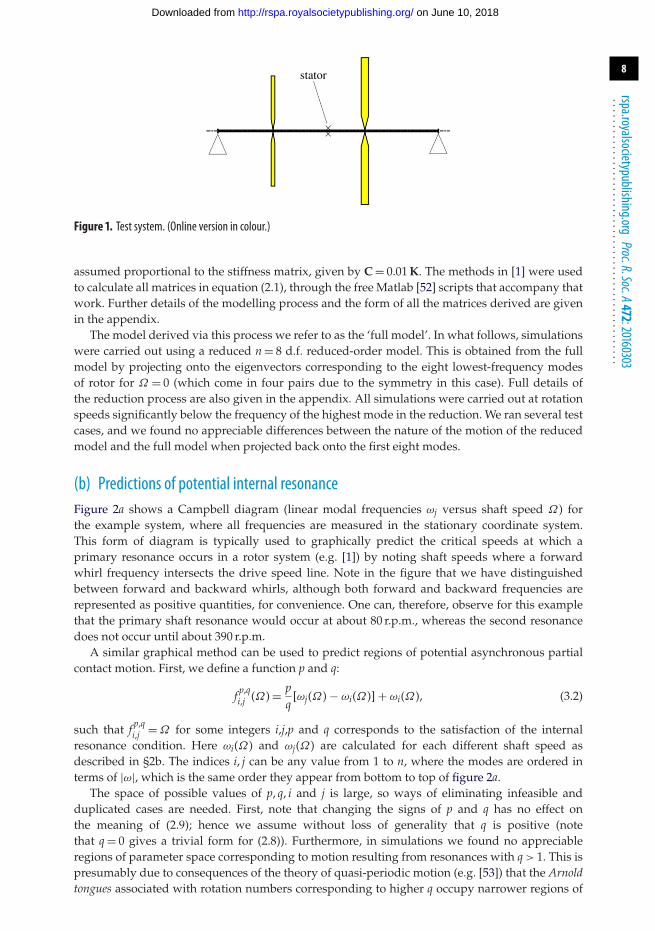
(a) Description and modellingThe system under consideration can be derived from the configuration shown in figure 1 whichconsists of a tube with two asymmetrically mounted, non-identical discs. The rotor is mountedon pinned bearings at each end of the shaft, with a stator in the form of a snubber ring, mountedat the centre of the shaft with a fixed clearance. The shaft is assumed to be constructed from asteel (E = 210 × 109 Pa, ν = 0.3) tube with 5 mm outer diameter and thickness 1 mm. The discs arealso made of steel with radii 0.15 m and 0.2 m and thicknesses 0.01 m and 0.02 m, respectively. Theshaft is 0.60 m long, with the smaller disc located 0.15 m from the left-hand end, and the largerdisc located 0.20 m from the right-hand end. The stator contact is modelled by assuming that thelateral vibrations of the shaft is subject to bilinear stiffness and damping. Specifically, the forceexerted by the stator is assumed to be given by
Fc =
⎧⎪⎪⎪⎪⎨⎪⎪⎪⎪⎩
−ks(r − δ)
{xc
yc
}/r − cs
{xc
yc
}, if r ≥ δ{
0
0
}, if r< δ,
(3.1)
where ks is the stator contact stiffness, cs the stator contact damping coefficient, xc and yc are thecoordinates of the shaft centre taken in the plane of the stator, δ is the clearance of the stator and
r =√
x2c + y2
c . In all cases presented here, δ = 1 × 10⁻³ m.Synchronous forcing is provided by a small off-centre eccentricity ε on the smaller disc. In
order to ensure that initial transients decay within a reasonable time period to the steady state,light damping is applied along the length of the shaft. This is assumed to be external damping,to avoid potential instabilities caused by internal damping [1].
The configuration is initially modelled using the finite-element method. The mesh for thismodel is in the form of a shaft-line model, that is, all nodes are located along the centre line ofthe shaft. Thirteen nodes are spaced equally along the shaft, with the degrees of freedom at eachnode being vertical and lateral translation and rotation. Therefore, the model has n = 48 d.f. wheretranslation degrees of freedom have been eliminated from the end nodes by the assumption ofpinned bearings. The shaft itself was represented by Timoshenko beam elements, and the discsby additional inertia terms at the nodes concerned. In all cases presented, the damping matrix was
on June 10, 2018http://rspa.royalsocietypublishing.org/Downloaded from
Figure 1. Test system. (Online version in colour.)
assumed proportional to the stiffness matrix, given by C = 0.01 K. The methods in [1] were usedto calculate all matrices in equation (2.1), through the free Matlab [52] scripts that accompany thatwork. Further details of the modelling process and the form of all the matrices derived are givenin the appendix.
The model derived via this process we refer to as the ‘full model’. In what follows, simulationswere carried out using a reduced n = 8 d.f. reduced-order model. This is obtained from the fullmodel by projecting onto the eigenvectors corresponding to the eight lowest-frequency modesof rotor for Ω = 0 (which come in four pairs due to the symmetry in this case). Full details ofthe reduction process are also given in the appendix. All simulations were carried out at rotationspeeds significantly below the frequency of the highest mode in the reduction. We ran several testcases, and we found no appreciable differences between the nature of the motion of the reducedmodel and the full model when projected back onto the first eight modes.
(b) Predictions of potential internal resonanceFigure 2a shows a Campbell diagram (linear modal frequencies ωj versus shaft speed Ω) forthe example system, where all frequencies are measured in the stationary coordinate system.This form of diagram is typically used to graphically predict the critical speeds at which aprimary resonance occurs in a rotor system (e.g. [1]) by noting shaft speeds where a forwardwhirl frequency intersects the drive speed line. Note in the figure that we have distinguishedbetween forward and backward whirls, although both forward and backward frequencies arerepresented as positive quantities, for convenience. One can, therefore, observe for this examplethat the primary shaft resonance would occur at about 80 r.p.m., whereas the second resonancedoes not occur until about 390 r.p.m.
A similar graphical method can be used to predict regions of potential asynchronous partialcontact motion. First, we define a function p and q:
f p,qi,j (Ω) = p
q[ωj(Ω) − ωi(Ω)] + ωi(Ω), (3.2)
such that f p,qi,j =Ω for some integers i,j,p and q corresponds to the satisfaction of the internal
resonance condition. Here ωi(Ω) and ωj(Ω) are calculated for each different shaft speed asdescribed in §2b. The indices i, j can be any value from 1 to n, where the modes are ordered interms of |ω|, which is the same order they appear from bottom to top of figure 2a.
The space of possible values of p, q, i and j is large, so ways of eliminating infeasible andduplicated cases are needed. First, note that changing the signs of p and q has no effect onthe meaning of (2.9); hence we assume without loss of generality that q is positive (notethat q = 0 gives a trivial form for (2.8)). Furthermore, in simulations we found no appreciableregions of parameter space corresponding to motion resulting from resonances with q> 1. This ispresumably due to consequences of the theory of quasi-periodic motion (e.g. [53]) that the Arnoldtongues associated with rotation numbers corresponding to higher q occupy narrower regions of
on June 10, 2018http://rspa.royalsocietypublishing.org/Downloaded from
Figure 2. (a) Campbell diagram for test system, showingwhirl frequencies in the stationary coordinate system. Crosses indicateforward whirls, circles indicate backward whirls. Dashed line indicates the shaft speed. (b) Evaluations of f p,qi.j (Ω ) as given byequation (3.2). Labels indicate the choice of parameters used for the adjacent curve. Dashed line indicates the shaft speed.(Online version in colour.)
parameter space and so are less likely to be excited in practice. Therefore, in what follows we onlyconsider the case q = 1. Another means of reducing the possible combinations is to note that if thechoice of modes i and j are swapped in (3.2), then the same equation is obtained if we swap p withq − p. To eliminate this duplication, we assume without loss of generality in (3.2) that j< i. Finally,cases where p = 1 or p = 0 are also omitted, because these give trivial forms of equation (2.9).
Evaluations of equation (3.2) were performed for values of p from −10 to 10. The results ofthis sweep are shown in figure 2b; note that many choices of p result in curves that lie outside theregion depicted. An intersection of a curve and the dashed line ω=Ω indicates that equation (2.9)is satisfied, and that therefore there is potential for internal resonance at that shaft speed.
It can be seen from figure 2b that there are numerous solutions to equation (2.9) in theregion shown. However, this analysis has only considered the underlying linear whirl speeds; inpractice, the detail of the mode shapes, damping, nonlinearity, non-conservative forces and initialconditions may all influence whether a partial contact orbit exists or is stable. More generally,in dynamical systems for which quasi-periodic motion is predicted by a linear or conservativeanalysis, it is known that internal resonances with sufficiently large Arnold tongues, in thepresence of nonlinearity and damping, typically lead to appreciable parameter intervals in whichthere is stable phase-locked periodic motion. By contrast, those resonances with narrow Arnoldtongues tend to not be excited (e.g. [53,54]). In our context, as nonlinearity only arises throughcontact, these phase-locked motions will necessarily be partial contact solutions. Owing to thenonlinear nature of these considerations, in practical situations we turn to numerical methodsto see which of these potential internal resonances lead to observable partial contact motion.
on June 10, 2018http://rspa.royalsocietypublishing.org/Downloaded from
(c) Numerical bifurcation methodologyBifurcation analysis is an invaluable framework for understanding nonlinear systems, byidentifying and classifying points at which their responses undergo qualitative changes [54].However, in cases such as this one with relatively little analytical knowledge of the underlyingsystem and its responses, and with the further complication of a discontinuous nonlinearity, thesimplest reliable means of obtaining a bifurcation diagram can be through conducting a largenumber of time-domain simulations. This approach, known as brute force bifurcation analysis, isadopted here.
At a given shaft speed, a randomized initial condition is created. A time simulation is thenrun for sufficient time for transients to decay. Simple properties are then used to quantify thefinal steady state motion—in this case, the motion is simply characterized by the maximum andminimum magnitude of displacement of the stator node during oscillation (note that a Poincaréanalysis as used in [38] cannot be used because we have no natural choice of the sampling period).For these tests, the minimum and maximum are taken over 250 drive rotations once the data havesettled.
The above procedure is repeated 25 times at each driving frequency; this effectively forms aMonte Carlo analysis of the stable steady state responses of the system at a given driving speed.A small step is then made in the shaft speed Ω and the process repeated, so that a completeone-parameter bifurcation diagram is obtained of solution response versus shaft speed.
To improve the performance of the simulation, the system was reduced to 8 d.f. (16 dimensionsof phase space) by projection onto the first 8 linear undamped mode shapes of the non-rotatingsystem. This includes all the major modes of the system; modes 9 and above are only linearlyexcited at much higher rotation speeds for for this system. The simulation itself was carried outin ODE45 in Matlab [52], with event detection used to locate changes between contacting andnon-contacting motion. The event detection function halted the simulation every time the radialdisplacement of the contact node crossed the clearance threshold, and then the simulation wouldbe restarted with optimal properties for the new state of contact or non-contact. Note that as partof this process, equation (3.1) requires that the radial displacement is evaluated at the contact node(which is a projection of linear modal vectors). Once contact has been established, the resultingforce must also transformed back to the reduced modal form.
The random initial condition was generated as follows. The state space vector was set to {0p0}T
where the reduced modal velocity vector p0 was populated with pseudo random numbers foreach time simulation, hence the initial conditions were zero displacement with a random velocity.This vector was then scaled so that the non-dimensional initial kinetic energy given by 1
2 pT0 p0 was
a constant value of 0.06 in each case.
4. ResultsWe present the results of the brute force bifurcation analysis for the example system, in twoextreme cases. First, in §4a, the results for a relatively soft stator, with no damping are presented.Here we tend to find a wide range of excited internal resonances. Then, in §4b, a perhaps morephysically realistic example (at least for laboratory implementation) is considered where thecontact stiffness is high in relation to the shaft stiffness, and impacts are dissipative. While thisappears to suppress many of the responses that occur in the previous case, partial contact orbitswith rich dynamics are still seen to occur.
(a) A low-stiffness snubber ringWe first present results where ks has the relatively low value of 1 × 10⁵ N m−1 and no dampingis applied in the stator i.e. cs = 0. Therefore, this represents a snubber-ring type stator which doesnot totally suppress motion beyond r = δ. Eccentricity is introduced by the off-centre distance ofdisc 1 being ε = 7.5 × 10⁻⁴ m.
on June 10, 2018http://rspa.royalsocietypublishing.org/Downloaded from
Figure 3. (a) Results of brute force bifurcation for ks = 1 × 10⁵ N m−1. (b) Detail of region 280–400 r.p.m. Labels indicatethe solution family that the response belong to. (Online version in colour.)
Figure 3 shows the results of the brute force bifurcation process as described in §3c. As can beseen, below 280 r.p.m. all markers coincide; as in all cases, the maximum and minimum r of theorbit are equal, it can be concluded that these cases always settle to synchronous whirling motion,where the radial displacement of the stator node remains constant. This motion is either linearforward (non-contacting) whirl, or in the case of the higher amplitude oscillations at 79–155 r.p.m.,constant-contact forward whirl. In the region of approximately 100–150 r.p.m., both solutions arestable and the initial condition determines which orbit will occur in steady state. It can be seenthat the linear forward whirl exists as a possible stable solution all the way up to 500 r.p.m.
At 280 r.p.m., a partial contact solution begins to occur, as shown by the presence of separateminimum and maximum markers in addition to those for the linear whirl case. The trace of thepartial contact orbit for 280 r.p.m. is depicted in figure 4a, which shows that while this motionseems orderly, it is not periodic in stationary coordinates; the pattern shown will continuallyprecess. However, figure 4b makes it clear that this motion is periodic and quite simple whenviewed in a rotating coordinate system. In order to better understand this orbit, a fast Fourier
on June 10, 2018http://rspa.royalsocietypublishing.org/Downloaded from
Figure 4. Steady-state partial contact orbit at drive speed 280 r.p.m. (a) Partial contact orbit in stationary coordinate system.Dotted-dashed line indicates the stator contact threshold. (a) Partial contact orbit in rotating coordinate system. Dotted-dashedline indicates the stator contact threshold. (c) FFT of lateral displacement in stationary coordinate system. (Online version incolour.)
transform (FFT) of the lateral displacement at the stator node in stationary coordinates ispresented in figure 4c, which shows that the three largest peaks are at 1.06 Hz, 1.80 Hz and 4.66 Hz.The first two of these are slightly greater in magnitude than the first forward and backwardwhirling frequencies of the rotor as shown in figure 2a, and 4.66 Hz corresponds to the drivingspeed. If we take ω1 = −1.06 × 2π rad s−1, and ω2 = 1.80 × 2π rad s−1, we find that these valuesapproximately satisfy (2.9) for p = 2. Hence this partial contact motion can be considered as aninternal resonance between the first forward and backward whirls. The reason that the whirlspeeds do not exactly match the linear predictions is believed to be that the nonlinearity inducedby the stator has a stiffening effect typical of weakly nonlinear systems [54]. This also causesthe onset of this motion to occur at the higher shaft speed of 280 r.p.m. compared with the 240r.p.m. predicted by figure 2b. Accurate modelling of this stiffening effect is left to future work.
on June 10, 2018http://rspa.royalsocietypublishing.org/Downloaded from
Figure 5. Detailed results from figure 3, solution S2,11,2 . (a,c,e) Orbits in rotating coordinate system at 302 r.p.m., 304 r.p.m. and312 r.p.m., respectively. (b,d,e) Excerpt of the time series of r at 302 r.p.m., 304 r.p.m. and 312 r.p.m., respectively. Dotted-dashedline indicates the stator contact threshold. (Online version in colour.)
All other peaks in figure 4 are much smaller in amplitude and can be shown to be the effect ofharmonics of the fundamental rotating coordinate system frequencies when translated into thestationary frame.
In fact, the ability of nonlinearity to alter the whirling frequencies has a more profound effect,in allowing this form of solution to exist over a wide range of frequencies. It can be seen fromfigure 3 that the partial contact orbit at 280 r.p.m. is part of a family of solutions, that can betraced by following the line of maxima and corresponding minima. At all points on this line,analysis of the orbits similar to that given above reveals them to consist of the first two whirlmodes, coupled with p = 2. Therefore, this entire family is solutions is given a label in figure 3 of
on June 10, 2018http://rspa.royalsocietypublishing.org/Downloaded from
Figure 6. Detailed results from figure 3, 360 r.p.m. (a) Orbit of S−1,12,3 solution in rotating coordinates. (b) FFT of lateral
displacement in stationary coordinates of S−1,12,3 solution (note there are twoclosely spacedpeaks, at 1.95 Hzand2.03 Hz). (c) Orbit
of QP solution in rotating coordinates. (d) FFT of QP solution. (Online version in colour.)
S2,11,2, where the subscripts and superscripts reflect the underlying whirling modes that constitute
the response, and the integers p and q, in the same was as used in equation (3.2). Note that byevaluating equation (2.8) with the given values, it may be seen that these responses are 2 : 1internal resonances in the rotating coordinate system.
By following the lines of maxima and minima in figure 3, it may be seen that solutionfamily S2,1
1,2 extends up to 397 r.p.m. However, it may be seen that there are discontinuities inthe amplitudes of responses as the drive speed increases. It emerges that these correspond tochange-of-period bifurcations, as seen in figure 5, which shows how the ‘kink’ in the line ofmaxima at 303 r.p.m. corresponds to a period-doubling. This shows how at 302 r.p.m. all contactsare identical, whereas at 303 r.p.m. there is a gentle oscillation in the maximum r that is reached.By 312 r.p.m. this has grown into alternate contacts being very different to each other. Thus, itcan be seen that substantially different responses can occur, but composed of the same form ofsynchronization of the underlying linear modes.
on June 10, 2018http://rspa.royalsocietypublishing.org/Downloaded from
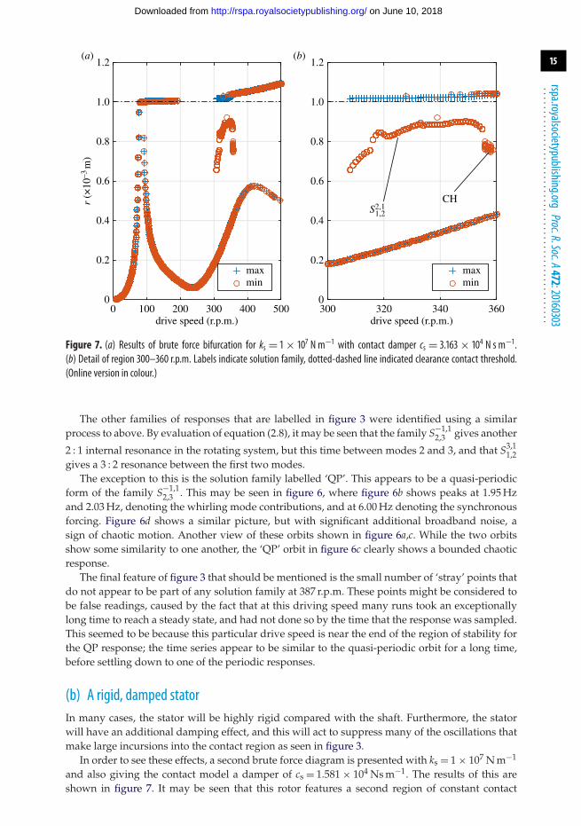
Figure 7. (a) Results of brute force bifurcation for ks = 1 × 10⁷ N m−1 with contact damper cs = 3.163 × 10⁴ N s m−1.(b) Detail of region 300–360 r.p.m. Labels indicate solution family, dotted-dashed line indicated clearance contact threshold.(Online version in colour.)
The other families of responses that are labelled in figure 3 were identified using a similarprocess to above. By evaluation of equation (2.8), it may be seen that the family S−1,1
2,3 gives another
2 : 1 internal resonance in the rotating system, but this time between modes 2 and 3, and that S3,11,2
gives a 3 : 2 resonance between the first two modes.The exception to this is the solution family labelled ‘QP’. This appears to be a quasi-periodic
form of the family S−1,12,3 . This may be seen in figure 6, where figure 6b shows peaks at 1.95 Hz
and 2.03 Hz, denoting the whirling mode contributions, and at 6.00 Hz denoting the synchronousforcing. Figure 6d shows a similar picture, but with significant additional broadband noise, asign of chaotic motion. Another view of these orbits shown in figure 6a,c. While the two orbitsshow some similarity to one another, the ‘QP’ orbit in figure 6c clearly shows a bounded chaoticresponse.
The final feature of figure 3 that should be mentioned is the small number of ‘stray’ points thatdo not appear to be part of any solution family at 387 r.p.m. These points might be considered tobe false readings, caused by the fact that at this driving speed many runs took an exceptionallylong time to reach a steady state, and had not done so by the time that the response was sampled.This seemed to be because this particular drive speed is near the end of the region of stability forthe QP response; the time series appear to be similar to the quasi-periodic orbit for a long time,before settling down to one of the periodic responses.
(b) A rigid, damped statorIn many cases, the stator will be highly rigid compared with the shaft. Furthermore, the statorwill have an additional damping effect, and this will act to suppress many of the oscillations thatmake large incursions into the contact region as seen in figure 3.
In order to see these effects, a second brute force diagram is presented with ks = 1 × 10⁷ N m−1
and also giving the contact model a damper of cs = 1.581 × 10⁴ Ns m−1. The results of this areshown in figure 7. It may be seen that this rotor features a second region of constant contact
on June 10, 2018http://rspa.royalsocietypublishing.org/Downloaded from
Figure 8. Time series and orbits of partial contact solutions from family S2,11,2 in figure 7, at various drive speeds. Dotted-dashedlines show the stator contact threshold. The crosses in (a,c,e,g) indicate where contact with the stator is established or broken.(Online version in colour.)
response beginning at approximately Ω = 350 r.p.m.; however, as the focus of this work is partialcontact response this is not discussed further. It is clear that the stiffer but less elastic contactshave had the effect of causing the majority of stable partial contact orbit solutions to disappear.
The remaining partial contact responses all derive from the same solution family S2,11,2, although
now it does not occur until a shaft speed of 308 r.p.m. is reached, highlighting that the predictionsof figure 2 become increasingly approximate as the harshness of the nonlinearity is increased.However, it may be noted that in this case the way that the response evolves as the driving speedincreases is different to the previous case. Figure 8 shows a series of time signals of r(t), with
on June 10, 2018http://rspa.royalsocietypublishing.org/Downloaded from
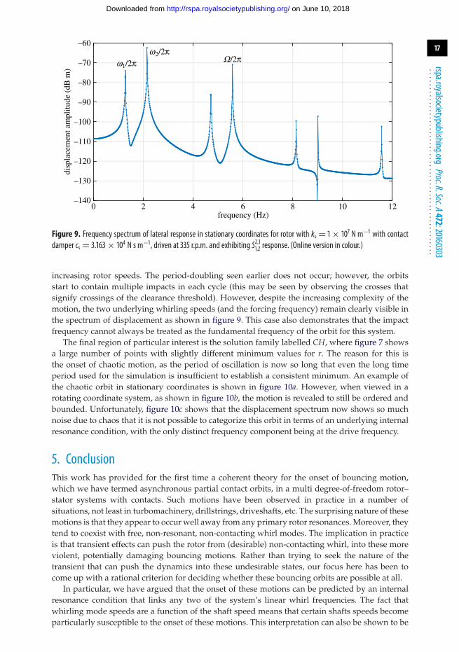
Figure 9. Frequency spectrum of lateral response in stationary coordinates for rotor with ks = 1 × 10⁷ N m−1 with contactdamper cs = 3.163 × 10⁴ N s m−1, driven at 335 r.p.m. and exhibiting S2,11,2 response. (Online version in colour.)
increasing rotor speeds. The period-doubling seen earlier does not occur; however, the orbitsstart to contain multiple impacts in each cycle (this may be seen by observing the crosses thatsignify crossings of the clearance threshold). However, despite the increasing complexity of themotion, the two underlying whirling speeds (and the forcing frequency) remain clearly visible inthe spectrum of displacement as shown in figure 9. This case also demonstrates that the impactfrequency cannot always be treated as the fundamental frequency of the orbit for this system.
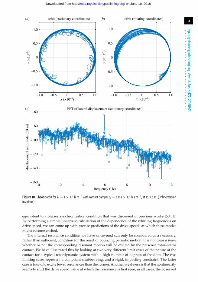
The final region of particular interest is the solution family labelled CH, where figure 7 showsa large number of points with slightly different minimum values for r. The reason for this isthe onset of chaotic motion, as the period of oscillation is now so long that even the long timeperiod used for the simulation is insufficient to establish a consistent minimum. An example ofthe chaotic orbit in stationary coordinates is shown in figure 10a. However, when viewed in arotating coordinate system, as shown in figure 10b, the motion is revealed to still be ordered andbounded. Unfortunately, figure 10c shows that the displacement spectrum now shows so muchnoise due to chaos that it is not possible to categorize this orbit in terms of an underlying internalresonance condition, with the only distinct frequency component being at the drive frequency.
5. ConclusionThis work has provided for the first time a coherent theory for the onset of bouncing motion,which we have termed asynchronous partial contact orbits, in a multi degree-of-freedom rotor–stator systems with contacts. Such motions have been observed in practice in a number ofsituations, not least in turbomachinery, drillstrings, driveshafts, etc. The surprising nature of thesemotions is that they appear to occur well away from any primary rotor resonances. Moreover, theytend to coexist with free, non-resonant, non-contacting whirl modes. The implication in practiceis that transient effects can push the rotor from (desirable) non-contacting whirl, into these moreviolent, potentially damaging bouncing motions. Rather than trying to seek the nature of thetransient that can push the dynamics into these undesirable states, our focus here has been tocome up with a rational criterion for deciding whether these bouncing orbits are possible at all.
In particular, we have argued that the onset of these motions can be predicted by an internalresonance condition that links any two of the system’s linear whirl frequencies. The fact thatwhirling mode speeds are a function of the shaft speed means that certain shafts speeds becomeparticularly susceptible to the onset of these motions. This interpretation can also be shown to be
on June 10, 2018http://rspa.royalsocietypublishing.org/Downloaded from
Figure 10. Chaotic orbit for ks = 1 × 10⁷ N m−1 with contact damper cs = 3.163 × 10⁴ N s m−1, at 357 r.p.m. (Online versionin colour.)
equivalent to a phasor synchronization condition that was discussed in previous works [50,51].By performing a simple linearized calculation of the dependence of the whirling frequencies ondrive speed, we can come up with precise predictions of the drive speeds at which these modesmight become excited.
The internal resonance condition we have uncovered can only be considered as a necessary,rather than sufficient, condition for the onset of bouncing periodic motion. It is not clear a prioriwhether or not the corresponding resonant motion will be excited by the presence rotor–statorcontact. We have illustrated this by looking at two very different limit cases of the nature of thecontact for a typical rotordynamic system with a high number of degrees of freedom. The twolimiting cases represent a compliant snubber ring, and a rigid, impacting constraint. The lattercase is found to excite fewer resonances than the former. Another weakness is that the nonlinearityseems to shift the drive speed value at which the resonance is first seen; in all cases, the observed
on June 10, 2018http://rspa.royalsocietypublishing.org/Downloaded from
drive speed seems to be slightly higher than predicted. This may be because of the basin ofattraction of the bouncing solution being vanishingly small at its point of onset. It may alsobe because of the effective stiffening caused by the nonlinearity. Finally, and most crucially, theinternal resonance criterion does not predict the range of Ω-values over which a particular classof bouncing orbit may exist, nor whether period-doubling or other routes to chaos may occur atthe high-Ω limit.
All of these more detailed questions require further nonlinear analysis. This is left to futurework. It is interesting to observe though that all orbits appear to bifurcate from their onset pointin the direction of increasing drive speed Ω . To establish this, and to gain insight into how theamplitude and characteristics of the bouncing orbits evolve as Ω is increased we have performedpreliminary calculations using two different methods. The first involves harmonic balance, whichapplies best in the case of a soft snubber-ring-type constraint. The second involves a rigid impactanalysis, using the discontinuity mapping methodology from the theory of piecewise-smoothdynamical systems (e.g. [55]). The results appear promising, but will be presented in detailelsewhere. Finally, experimental verification of the theory presented here is pressing, anotheravenue we are actively pursuing.
Authors’ contributions. A.D.S. developed the simulations that led to these results, with technical oversight fromM.I.F. A.R.C. conceived the brute-force bifurcation approach and discussion between all authors led to theinterpration of results as internal resonance phenomena. All authors participated in the prepration andapproval of the final manuscript.Competing interests. We declare we have no competing interests.Funding. The research leading to these results has received funding from the EPSRC grant ‘Engineeringnonlinearity’ EP/G036772/1.Acknowledgements. We acknowledge useful conversations with Andrea Zilli, Karin Mora and Joachim Sihler.
Appendix A. Details of matrix derivations
(a) SystemmatricesThe system is modelled following [1], by adapting the Matlab [52] scripts that accompany thiswork. The system is a shaft line model where each node k has 4 d.f.:
qk = [uk, vk, θk,ψk]T, (A 1)
which are illustrated in figure 11. The shaft consists of two-node beam elements, hence eachelement has degrees of freedom:
qe = [uk, vk, θk,ψk, uk+1, vk+1, θk+1,ψk+1]T. (A 2)
The shaft is assumed to be a Timoshenko beam neglecting rotary inertia hence the elementstiffness matrix is
Ke = EI(1 + φ)L3
⎡⎢⎢⎢⎢⎢⎢⎢⎢⎢⎢⎢⎢⎢⎢⎢⎣
12 0 0 6L −12 0 0 6L
0 12 −6L 0 0 −12 −6L 0
0 −6L (4 + φ)L2 0 0 6L (2 − φ)L2 0
6L 0 0 (4 + φ)L2 −6L 0 0 (2 − φ)L2
−12 0 0 −6L 12 0 0 −6L
0 −12 6L 0 0 12 6L 0
0 −6L (2 − φ)L2 0 0 6L (4 + φ)L2 0
6L 0 0 (2 − φ)L2 −6L 0 0 (4 + φ)L2
⎤⎥⎥⎥⎥⎥⎥⎥⎥⎥⎥⎥⎥⎥⎥⎥⎦
, (A 3)
on June 10, 2018http://rspa.royalsocietypublishing.org/Downloaded from
Equations (A 3)–(A 5) are combined in the usual way to obtain K, M and G. Furthermore, fornodes where discs are located, an addition to the mass matrix is made
Md =
⎡⎢⎢⎢⎣
Md 0 0 00 Md 0 00 0 Id 00 0 0 Id
⎤⎥⎥⎥⎦ (A 6)
at the appropriate degrees of freedom, and an addition to the gyroscopic matrix is also made
Gd =
⎡⎢⎢⎢⎣
0 0 0 00 0 0 00 0 0 Ip
0 0 −Ip 0
⎤⎥⎥⎥⎦ (A 7)
In equations (A 6) and (A 7), Md is the mass of the disc, Id is the disc’s moment of inertia aboutthe lateral axes and Ip is its moment of inertia about the z-axis. The assumption of simple pinnedbearings means that these can be implemented simply by removing the relevant translationaldegrees of freedom from all matrices. The damping matrix is assumed proportional to the stiffnessmatrix, hence C = 0.01K.
The system is assumed to have an off-centre displacement on the smaller disc equal to ε =0.75 × 10⁻³m. Hence forcing vector b0 is given as
b0 = εMd1[0 · · · 0 1 − i 0 · · · 0]T, (A 8)
where Md1 is the mass of the disc concerned, and the two non-zero terms occur at the degrees offreedom relating to displacement of the smaller disc.
For this system, given the arrangement of the degrees of freedom, the transformation matrixfrom rotating coordinates T used in (2.2) is a block diagonal matrix, where each block is thefollowing:
Tk(Ωt) =[
cosΩt − sinΩtsinΩt cosΩt
], (A 9)
which when substituted into the equation of motion gives
G = G + 2MJ, (A 10)
K = K −Ω2M +Ω2GJ (A 11)
and Kc =ΩCJ, (A 12)
where J is a block diagonal matrix where the block elements are[ 0 −1
1 0
]i.e.
J =
⎡⎢⎢⎢⎢⎢⎢⎣
0 −1 0 0 · · ·1 0 0 00 0 0 −10 0 1 0...
. . .
⎤⎥⎥⎥⎥⎥⎥⎦
. (A 13)
on June 10, 2018http://rspa.royalsocietypublishing.org/Downloaded from
(b) Reduced matrices for numerical simulationIn order to perform numerical simulation, as part of the brute force bifurcation method in §3c, thesystem is reduced using non rotating modes. The transformed variable p is related to q by
q = Φp, (A 14)
where Φ is formed by the first 8 mass normalized eigenvectors of M−1K; note that these will havefour separate eigenvalues, each repeated twice due to symmetry between x and y directions ofthe structure. Hence transforming equation (2.1) gives
p +ΩΦTGΦp + ΦTKΦp + ΦTCΦp + ΦTN(Φp, Φp) = ΦT�(Ω2b0 eiΩt). (A 15)
The values of the reduced matrices are as follows:
where diag([· · · ]) gives a diagonal matrix where the diagonal terms are the elements of the rowvector.
Noting that only the translational degrees of freedom at the stator node participate in thenonlinearity defined in equation (3.1), the nonlinear term in equation (A 15) can be reduced asfollows:
ΦTN(Φp, Φp) = ΦTc Fc(Φcp, Φcp), (A 19)
where Φc consists of the two rows of Φ relating to the translational displacements (u and v) at thestator node:
This matrix is also used when projecting the results of simulation back to the displacements at thestator node, as is done in all results figures.
In a similar manner to the reduction of the nonlinear term, the forcing term can be reduced bynoting that it only affects translational degrees of freedom at the node of the smaller disc. Hence,
ΦTRe(Ω2b0 eiΩt) = ΦTf Re(Ω2bf eiΩt), (A 21)
where bf consists of the two non-zero elements of b0 and Φf consists of the two rows of Φ relatingto the forced degrees of freedom:
2. Vance JM. 1988 Rotordynamics of turbomachinery. New York, NY: John Wiley & Sons.3. Friswell MI, Champneys AR. 2003 Defective systems and pseudospectra. Mater. Sci. Forum
440–441, 287–294. (doi:10.4028/www.scientific.net/MSF.440-441.287)4. Green K, Champneys AR, Friswell MI. 2006 Analysis of the transient response of an
automatic dynamic balancer for eccentric rotors. Int. J. Mech. Sci. 48, 274–293. (doi:10.1016/j.ijmecsci.2005.09.014)
5. Ishida T, Nagasaka I, Inoue T, Lee S. 1996 Forced oscillations of a vertical continuous rotorwith geometric nonlinearity. Nonlinear Dyn. 11, 107–120. (doi:10.1007/BF00044997)
6. Shaw J, Shaw SW. 1991 Non-linear resonance of an unbalanced rotating shaft with internaldamping. J. Sound Vib. 147, 435–451. (doi:10.1016/0022-460X(91)90492-3)
7. Adiletta G, Guido A, Rossi C. 1996 Chaotic motions of a rigid rotor in short journal bearings.Nonlinear Dyn. 10, 251–269. (doi:10.1007/BF00045106)
8. Jing JP, Meng G, Sun Y, Xia SB. 2005 On the oil-whipping of a rotor-bearing system by acontinuum model. Appl. Math. Model. 29, 461–475. (doi:10.1016/j.apm.2004.09.003)
9. de Castro HF, Cavalca KL, Nordmann R. 2008 Whirl and whip instabilities in rotor-bearing system considering a nonlinear force model. J. Sound Vib. 317, 273–293. (doi:10.1016/j.jsv.2008.02.047)
10. Patel TH, Darpe AK. 2008 Influence of crack breathing model on nonlinear dynamics of acracked rotor. J. Sound Vib. 311, 953–972. (doi:10.1016/j.jsv.2007.09.033)
11. Bonello P, Brennan MJ, Holmes R. 2004 A study of the nonlinear interaction between aneccentric squeeze film damper and an unbalanced flexible rotor. Trans. ASME J. Eng. GasTurbines Power 126, 855–866. (doi:10.1115/1.1787503)
12. Rodrigues DJ, Champneys AR, Friswell MI, Wilson R. 2011 Two-plane automatic balancing:a symmetry breaking analysis. Int. J. Nonlinear Mech. 46, 1139–1154. (doi:10.1016/j.ijnonlinmec.2011.04.033)
13. Rodrigues DJ, Champneys AR, Friswell MI, Wilson RE. 2011 Experimental investigation of asingle-plane automatic balancing. J. Sound Vib. 330, 385–403. (doi:10.1016/j.jsv.2010.08.020)
14. Jacquet-Richardet G. et al. 2013 Rotor to stator contacts in turbomachines. review andapplication. Mech. Syst. Signal Process. 40, 401–420. (doi:10.1016/j.ymssp.2013.05.010)
15. Jansen JD. 1991 Non-linear rotor dynamics as applied to oilwell drillstring vibrations. J. SoundVib. 147, 115–135. (doi:10.1016/0022-460X(91)90687-F)
16. Ahmad S. 2010 Rotor casing contact phenomenon in rotor dynamics literature survey. J. Vib.Control 16, 1369–1377. (doi:10.1177/1077546309341605)
17. Chiba A, Fukao T, Ichikawa O, Oshima M, Takemoto M, Dorrell DG. 2005 Magnetic bearingsand bearingless drives. Amsterdam, The Netherlands: Elsevier.
18. Bleuler H, Cole M, Keogh P, Larsonneur R, Maslen E, Okada Y, Schweitzer G, Traxler A.2009 Magnetic bearings: theory, design, and application to rotating machinery. Berlin, Germany:Springer.
19. Schweitzer G. 2005 Safety and reliability aspects for active magnetic bearing applications-a survey. Proc. Inst. Mech. Eng. I J. Syst. Control Eng. 219, 383–392. (doi:10.1243/095965105X33491)
20. Ehrich FF. 2008 Observations of nonlinear phenomena in rotordynamics. J. Syst. Des. Dyn. 2,641–651. (doi:10.1299/jsdd.2.641)
21. Newkirk B, Taylor H. 1926 Shaft rubbing: relative freedom of rotor shafts from sensitivenessto rubbing contact when running above their critical speeds. Mech. Eng. 48, 830–832.
22. Black HF. 1968 Interaction of a whirling rotor with a vibrating stator across a clearanceannulus. J. Mech. Eng. Sci. 10, 1–12. (doi:10.1243/JMES_JOUR_1968_010_003_02)
23. Ehrich FF. 1969 The dynamic stability of rotor/stator radial rubs in rotating machinery. J. Eng.Ind. 91, 1025–1028. (doi:10.1115/1.3591743)
25. Jiang J. 2007 The analytical solution and the existence condition of dry friction backward whirlin rotor-to-stator contact systems. J. Vib. Acoust. 129, 260–264. (doi:10.1115/1.2345677)
26. Vlajic N, Liu X, Karki H, Balachandran B. 2014 Torsional oscillations of a rotor with continuousstator contact. Int. J. Mech. Sci. 83, 65–75. (doi:10.1016/j.ijmecsci.2014.03.025)
27. Richard T, Germay C, Detournay E. 2004 Self-excited stick–slip oscillations of drill bits. C. R.Mec. 332, 619–626. (doi:10.1016/j.crme.2004.01.016)
28. Germay C, Denoël V, Detournay E. 2009 Multiple mode analysis of the self-excited vibrationsof rotary drilling systems. J. Sound Vib. 325, 362–381. (doi:10.1016/j.jsv.2009.03.017)
on June 10, 2018http://rspa.royalsocietypublishing.org/Downloaded from
29. Leine R, Van Campen D, Keultjes W. 2002 Stick-slip whirl interaction in drillstring dynamics.J. Vib. Acoust. 124, 209–220. (doi:10.1115/1.1452745)
30. Liu X, Vlajic N, Long X, Meng G, Balachandran B. 2013 Nonlinear motions of a flexiblerotor with a drill bit: stick-slip and delay effects. Nonlinear Dyn. 72, 61–77. (doi:10.1007/s11071-012-0690-x)
31. Ehrich FF. 1972 Sum and difference frequencies in vibration of high speed rotating machinery.J. Eng. Ind. 94, 181–184. (doi:10.1115/1.3428109)
32. Ehrich FF, O‘Connor J. 1967 Stator whirl with rotors in bearing clearance. J. Eng. Ind. 89,381–389. (doi:10.1115/1.3610057)
33. Neilson R, Barr A. 1988 Dynamics of a rigid rotor mounted on discontinuously non-linearelastic supports. Proc. Inst. Mech. Eng. C J. Mech. Eng. Sci. 202, 369–376. (doi:10.1243/PIME_PROC_1988_202_135_02)
34. Szczygielski W. Application of chaos theory to the contacting dynamics of high-speed rotors.In Rotating machinery dynamics, pp. 319–326.
35. Ehrich FF. 1988 High order subharmonic response of high speed rotors in bearing clearance.J. Vib. Acoust. Stress Reliab. Des. 110, 9–16. (doi:10.1115/1.3269488)
36. Muszynska A, Goldman P. 1995 Chaotic responses of unbalanced rotor/bearing/statorsystems with looseness or rubs. Chaos Solitons Fractals 5, 1683–1704. (doi:10.1016/0960-0779(94)00171-L)
37. Chu F, Zhang Z. 1998 Bifurcation and chaos in a rub-impact jeffcott rotor system. J. Sound Vib.210, 1–18. (doi:10.1006/jsvi.1997.1283)
38. Edwards S, Lees A, Friswell MI. 1999 The influence of torsion on rotor/stator contact inrotating machinery. J. Sound Vib. 225, 767–778. (doi:10.1006/jsvi.1999.2302)
39. Karpenko EV, Wiercigroch M, Pavlovskaia EE, Cartmell MP. 2002 Piecewise approximateanalytical solutions for a jeffcott rotor with a snubber ring. Int. J. Mech. Sci. 44, 475–488.(doi:10.1016/S0020-7403(01)00108-4)
40. Karpenko EV, Wiercigroch M, Cartmell MP. 2002 Regular and chaotic dynamics of adiscontinuously nonlinear rotor system. Chaos Solitons Fractals 13, 1231–1242. (doi:10.1016/S0960-0779(01)00126-6)
41. Pavlovskaia EE, Karpenko E, Wiercigroch M. 2004 Non-linear dynamic interactions ofa jeffcott rotor with preloaded snubber ring. J. Sound Vib. 276, 361–379. (doi:10.1016/j.jsv.2003.07.033)
42. Karpenko E, Wiercigroch M, Pavlovskaia EE, Neilson R. 2006 Experimental verification ofjeffcott rotor model with preloaded snubber ring. J. Sound Vib. 298, 907–917. (doi:10.1016/j.jsv.2006.05.044)
43. Chu F, Lu W. 2005 Experimental observation of nonlinear vibrations in a rub-impact rotorsystem. J. Sound Vib. 283, 621–643. (doi:10.1016/j.jsv.2004.05.012)
44. Torkhani M, May L, Voinis P. 2012 Light, medium and heavy partial rubs during speedtransients of rotating machines: numerical simulation and experimental observation. Mech.Syst. Signal Process. 29, 45–66. (doi:10.1016/j.ymssp.2012.01.019)
45. Kim Y-B, Noah S. 1996 Quasi-periodic response and stability analysis for a non-linear jeffcottrotor. J. Sound Vib. 190, 239–253. (doi:10.1006/jsvi.1996.0059)
46. Von Groll G, Ewins DJ. 2001 The harmonic balance method with arc-length continuation inrotor/stator contact problems. J. Sound Vib. 241, 223–233. (doi:10.1006/jsvi.2000.3298)
47. Cole M, Keogh P. 2003 Asynchronous periodic contact modes for rotor vibration within anannular clearance. Proc. Inst. Mech. Eng. C J. Mech. Eng. Sci. 217, 1101–1115. (doi:10.1243/095440603322517126)
48. Keogh P, Cole M. 2003 Rotor vibration with auxiliary bearing contact in magnetic bearingsystems part 1: synchronous dynamics. Proc. Inst. Mech. Eng. C J. Mech. Eng. Sci. 217, 377–392.(doi:10.1243/095440603321509676)
49. Kora K, Budd C, Glendinning P, Keogh P. 2014 Non-smooth Hopf-type bifurcations arisingfrom impact-friction contact events in rotating machinery. Proc. R. Soc. A 470, 20140490.(doi:10.1098/rspa.2014.0490)
50. Zilli A, Williams RJ, Ewins DJ. 2015 Nonlinear dynamics of a simplified model of anoverhung rotor subjected to intermittent annular rubs. J. Eng. Gas Turbines Power 137, 065001.(doi:10.1115/1.4028844)
51. Shaw AD, Barton DAW, Champneys AR, Friswell MI. 2016 Dynamics of an mdof rotor statorcontact system. In Proc. of the 34th IMAC, a Conf. on Structural Dynamics, Orlando, FL, 25–28January.
on June 10, 2018http://rspa.royalsocietypublishing.org/Downloaded from
52. Matlab and simulink for technical computing (July 2012). See http://www.mathworks.com.53. Arrowsmith D, Place C. 1990 An introduction to dynamical systems. Cambridge, UK: Cambridge
University Press.54. Strogatz SH. 2014 Nonlinear dynamics and chaos: with applications to physics, biology, chemistry,
and engineering. Boulder, CO: Westview Press.55. di Bernardo M, Budd C, Champneys AR, Kowalczyk P. 2008 Piecewise-smooth dynamical
systems; theory and applications. Berlin, Germany: Springer.
on June 10, 2018http://rspa.royalsocietypublishing.org/Downloaded from