(At Least) Four Theoriesfor Sovereign Default:

An Empirical EvaluationMarkus Eberhardt∗

School of Economics, University of Nottingham, UKCentre for Economic Policy Research, UK

July 29, 2021

Abstract: Why do some sovereigns repay their debts while others default? I empirically in-

vestigate four prominent theories for default (or its avoidance): (i) reputation, (ii) punishment,

(iii) domestic politics, and (iv) international spillovers. Adopting an early warning system

(EWS) approach for a large sample of developing and emerging economies (1970-2015) I find

that reputation and spillover effects dominate in terms of economic significance. In robust-

ness checks I allow for the transmission of each theory strand through macro-fundamentals,

account for capital controls, debt relief, and capital flow bonanzas, investigate domestic, pri-

vate and present-value external debt, and conduct sample splitting exercises (by exchange rate

arrangement, political regime, financial development, and time period). Though they provide

more refined insights into the differential mechanisms at work, none of these exercises substan-

tially alter the above conclusions.

JEL Classification: F34, F41, G15, H63

Keywords: sovereign default, public debt, developing and emerging economies, international

capital markets, reputation, punishment, domestic politics, spillovers, early warning system

∗This research was initiated while I was a Visiting Economist in the IMF SPR Department. The views expressedin this paper are my own and do not necessarily represent those of the IMF or IMF policy. Marta Aloi, RodolpheDesbordes, William Gatt, David Gill, Oliver Morrissey, Andrea Presbitero, Tobias Schilling, and seminar/sessionparticipants and discussants at NICEP/University of Nottingham, the CSAE Annual Conference in Oxford, theMMF Conference in Edinburgh, and SKEMA Business School in Paris provided constructive comments and sug-gestions which are gratefully acknowledged. I thank Cecilia Testa for pointing me to various political sciencedatasets; Fabian Valencia for sharing updated data on systemic financial crises; Luis Catão and Rui Mano for mak-ing the data for their 2017 paper available online; and Daniel Dias, Christine Richmond and Mark Wright for accessto the external debt data they created for their 2014 paper. The usual disclaimers apply. Correspondence: MarkusEberhardt, School of Economics, Sir Clive Granger Building, University Park, Nottingham NG7 2RD, UK. Email:markus.eberhardt@nottingham.ac.uk

1

1 Introduction

Are sovereign defaults accidents brought about by precarious macroeconomic fundamentals

and triggered by unanticipated shocks, or do governments chose to default as the result of

strategic calculation? Are sovereigns kept in check by threats and implicit gunboat tactics,

by concerns over their reputation and future lending conditions, or by democratically elected

governments worried about the next (opinion) polls? What about sovereign default in a glob-

alised world, where macroeconomic vulnerability may spill across economies, or where the

presence of common lenders entices sovereigns to default and renegotiate when they observe

other economies doing so? No doubt multiple factors such as these are at play, but which are

the empirically dominant mechanisms?

The existing empirical literature on sovereign default and bond spreads with reference to

emerging and developing economies is very rich, but typically focuses on a relatively small set

of factors related to macroeconomic fundamentals (Manasse and Roubini, 2009), foreign liabil-

ities (Catão and Milesi-Ferretti, 2014), concerns over loss of reputation (Catão and Mano, 2017),

political regime and institutions (Archer et al., 2007; Van Rijckeghem and Weder, 2009; Beaulieu

et al., 2012), or economic reprisals (Rose, 2005; Fuentes and Saravia, 2010) among others. Even

measures for the two dominant theoretical explanations in the economics literature (reputation

and punishment, see Bulow and Rogoff, 2015) are rarely entered into the same empirical model

to gauge their comparative explanatory power.1

In this study I use an ‘early warning system’ approach to empirically investigate four

theories for sovereign default or its avoidance: (i) concerns over a sovereign’s international

reputation, i.e. being branded as a ‘serial defaulter,’ with implications for future lending con-

ditions (Eaton and Gersovitz, 1981; Tomz, 2007); (ii) the deterrence effect of external threats,

sanctions and other forms of reprisal (Bulow and Rogoff, 1988, 1989); (iii) the domestic political

system: differential behaviour of autocracies versus democracies, and within the latter the im-

pact of change in political stability (Archer et al., 2007; Beaulieu et al., 2012); and (iv) a ‘domino

effect’ of international crisis spillovers with default either an inevitability or a strategic choice

(Elliott et al., 2014; Acemoglu et al., 2015; Arellano et al., 2017).

These four strands comprise the two explanations dominating the economics literature

(reputation and punishment), one favoured in political science (political system), and a more

recent explanation reflecting on the embeddedness of sovereign lending in an international net-

work of lenders and borrowers (spillovers).2 In addition to these four strands I include macro-

economic fundamentals (e.g. debt stock and debt service flows, inflation, foreign reserves) and1A notable exception is Benczúr and Ilut (2016).2It should be noted that Bulow and Rogoff (1988) already consider a broader international relations framework

which leads to enforcement mechanisms other than the direct punishment approach. See Section 2.4 for other earlyinvestigations of spillovers.

2

consider a large number of additional factors (e.g. conflict, financial crises, exchange rate ar-

rangements). As will become clearer when I motivate robustness checks and alternative data

series employed, there are a great many more theories of default and its avoidance underpin-

ning these additional analyses, and I attempt to do them justice while maintaining the focus on

the four considered most prominently by the existing literature.

I carry out this investigation with a common empirical framework so as to compare

and contrast the salience and (in the statistical sense) power of the above factors in predicting

sovereign defaults. After introducing each theory I operationalise them for empirical investiga-

tion alongside standard macroeconomic controls in a panel of up to 114 developing countries

for 1970 to 2015. I adopt and extend existing empirical approaches from the bond spreads and

financial crisis literatures to proxy reputation, political economy and spillover effects, while

introducing a number of novel empirical measures for the threat of direct punishment, centred

around the evolution of trade costs and of membership in regional trade agreements.

My empirical implementation, a Mundlak-Chamberlain extension to the random effects

logit model (recently applied in Caballero, 2016, for the analysis of banking crises), also known

as a ‘correlated random effects’ model, allows me to predict sovereign default events while

keeping observations from countries which never defaulted in the sample. This is in con-

trast to the standard conditional logit model widely applied in empirical crisis prediction (e.g.

Kaminsky and Vega-Garcia, 2016): excluding non-crisis countries is an awkward starting point

(clearly subject to concerns over sample selection) if the aim of the exercise is to quantify the

effects of different variables on the propensity of default.3

Critics will be swift to point out that treating a set of macroeconomic fundamentals as

seemingly unconnected to the alternative theories for default is naïve and likely a source of

bias. Furthermore, reputation, threats and incentives, domestic politics, and spillovers may

affect all crisis predictors in some countries but not in others, with a pooled analysis merely in-

cluding these measures as covariates likely to miss these heterogeneities. Alternatively, jointly

controlling for factors like political regime and reputation may be introducing a ‘bad control’,

where one factor is causally downstream from another and hence blocking their direct effect

on default. This aside, the recent literature on financial crises more generally has pointed to

a number of ‘external’ variables related to global commodity price fluctuations and capital in-

flows, among others, which arguably have a significant bearing on the vulnerability to debt

crises as well (e.g. Caballero, 2016; Eberhardt and Presbitero, 2021). Finally, measures of public

indebtedness are likely misleading if they do not account for domestic debt or private debt or

3Does this empirical choice matter? I find that a number of covariates are statistically insignificant in the smallerdefaulter-only sample. Comparing effect sizes (marginal effect of a 1sd increase in x relative to the unconditionaldefault probability in the full and defaulters-only samples, respectively) results differ substantially for reputation,punishment, and political effects, as well as macro-fundamentals, but not for international spillovers. Relative effectsize between full and defaulters-only samples vary between 33% and 240% for individual covariates.

3

if external debt is measured at face value.

I attempt to address these concerns by (i) allowing for interaction effects between some

macroeconomic fundamentals and measures for the four default theories;4 (ii) analysing the

changes in results when selective strands are omitted (to ward against bad controls) while also

studying minimalist specifications to establish whether plausible proxies offer any predictive

power on their own; (iii) conducting a number of sample splitting exercises based on a coun-

try’s political regime, exchange rate arrangement, level of financial development, as well as

by time period; (iv) adding additional controls to the benchmark model to capture changes in

capital controls, commodity price movements, the HIPC (highly indebted poor countries) debt

relief initiative, hyper-inflation, or capital inflow bonanzas; and (v) conducting my analysis

with data for total debt (Abbas et al., 2010), private debt (Mbaye et al., 2018), and external debt

stock in present value terms (Dias et al., 2014), respectively.

My findings for each theory strand in isolation suggest that reputation, threats and incen-

tives, domestic politics, and spillovers can play an important role in (self-)disciplining govern-

ments. When I analyse these strands in an early warning system approach alongside macroe-

conomic fundamentals I find that reputation as well as spillover effects dominate in terms of

economic magnitudes, followed by a number of macroeconomic fundamentals. Empirical ev-

idence for domestic politics and threats/incentives is weaker.5 These findings are robust to

a battery of additional controls, as well as the use of alternative measures for indebtedness.

While much of the economics and political science literature has focused on its own preferred

explanations — reputation and punishment for the former, (domestic) politics in the latter — it

would appear that the relatively less appreciated fourth theory strand on spillovers is of great

significance and thus warrants the recent focus in theoretical work (Cole et al., 2016; Arellano

et al., 2017).

The remainder of the paper is organised as follows: in Section 2 I review the literature

on the four theories for sovereign default. In Section 3 I introduce the data and carry out basic

descriptive analysis. The empirical model and implementation are introduced in Section 4.

Results are presented and discussed in Section 5, Section 6 concludes.

4This setup can for instance account for a situation where ‘bad reputation’ or ‘direct punishment’ work throughrestricted access to international financial markets, thus affecting debt stock.

5I cannot rule out that these aspects are adversely affected by the inclusion of the spillover variables, whichmay wash out subtler effects. However, alternative models adopting a split by political regime, in contrast tothe evidence for splits by exchange rate regimes or level of financial development, do not show any significantdifferences in crisis determinants between autocracies and democracies.

4

2 Four Theories of Sovereign Default

Sovereign lending is conducted in an environment of limited enforcement: given the very na-

ture of sovereignty, creditors are limited in their ability to seize assets inside a debtor country

when the latter defaults on a loan. Sovereign default has been taking place for centuries, but

to date no dominant “clear and coherent answer” (Bulow and Rogoff, 2015) to the question

what foreign creditors can do when sovereigns default — and relatedly, why some countries

default and others do not — has emerged. At least four broad strands of explanations have

been proposed in the literature, reviewed in turn below, followed by variations and ‘other’

determinants.

2.1 International Reputation: ‘Serial Defaulters’

This strand of theory is most closely associated with the seminal paper by Eaton and Gerso-

vitz (1981). Sovereign borrowing and repayment is only related to consumption smoothing

(the mechanism) and concerns over reputation (the motivation), whereas external threats and

the governing law of the debt is irrelevant. This setup also implies that political regime and

institutions do not play any role in the model. As a result, debtors repay their debt in good

times and scramble to borrow more in bad times; default only occurs in good times, since the

consumption smoothing mechanism of sovereign lending necessitates continued borrowing in

‘bad states’ — this theoretical prediction makes for a nice link with the empirical question about

‘default in bad times’ raised by Tomz and Wright (2007) among others.

Mike Tomz’ (2007) book Reputation and International Cooperation provides a detailed mo-

tivation for a variation on the reputation theme, categorising borrowers into ‘stalwarts’ (goodie

two-shoes), ‘fair-weather’ (repay in good times) and ‘lemons’ (default in bad times and occa-

sionally in good times as well). On the basis of observed actions creditors may form and update

beliefs about a sovereign’s default probability, which constitutes the latter’s reputation. Types

and hence reputations are not fixed and Tomz (2007) acknowledges that domestic politics may

change priorities and thus the perceived importance of reputation. The rich empirical evidence

he presents in support of the reputation theory (and against the punishment theory) is based

on historical subperiods and geographical subsamples dealing with each motivation to repay

separately — Tomz (2007) is thus unable to empirically test both theories jointly.

Alfaro and Kanczuk (2005) provide a theoretical model in which some equilibria imply

countries delay default (they ‘muddle through’) due to concerns over their reputation: a ‘good’

government can signal its type by enduring a recession and thus securing favourable condi-

tions for future lending.

Gelos et al. (2011) empirically study access to international credit markets and find little

5

evidence for detrimental reputation effects from default frequency, provided renegotiations are

completed relatively swiftly. Catão and Mano (2017) study the ‘default premium puzzle,’ the

phenomenon that countries with a history of, and hence a reputation for, default only seem to

pay small interest rate premia for subsequent borrowing. They construct a number of ‘memory

variables’ which capture the historical prevalence and recency of default for each country and

encompass the existing metrics for default premium estimation. Equipped with these proxies

they are able to establish a substantial reputational default premium for historical and modern-

day samples (250 and 350 basis points in the first years of market re-entry, respectively).

2.2 Default and (the Threat of) Direct Punishment

This strand is closely associated with the theoretical work by Bulow and Rogoff (1988, 1989).

Here, creditors have rights in foreign creditor-country courts, i.e. if country A borrows from

bank i in country B, defaults on i’s loan and proceeds to borrow from bank j in the same coun-

try, then bank i can stake a claim on being repaid from the loan by bank j (Bulow and Rogoff,

2015). This incentivises the sovereign to repay old debts before borrowing again. Creditors

are thus afforded legal rights to interfere in the commercial dealings of the borrowers, e.g. by

sanctioning trade outright, seizing shipments, or creating serious trade frictions by regulatory

means.

Jayachandran and Kremer (2006) highlight the inefficiency of trade sanctions (due to in-

centives for evasion, self-harm to the creditor, harm to the target country’s population rather

than its politicians) and with an eye on the ‘regime type’ explanation discussed below suggest

a mechanism of ‘loan sanctions’ to break a spiralling ‘odious debt’ cycle by a repressive regime.

Bulow and Rogoff (2015) however argue that the potential for self-harm and other considera-

tions are “precisely the kind of issue that a bargaining theoretic framework [like theirs] allows

one to approach.”

The analysis in Tomz (2007) offers a variety of arguments and empirical evidence against

the direct punishment explanation — most notably his use of text search to show that any

mention of ‘sanctions’ is virtually absent in tens of thousands of newspaper clippings compiled

by the British Corporation for Foreign Bondholders for the period of the ‘First Globalisation’ (1870-

1914). This and other findings make it somewhat harder to argue the direct punishment case.

Detailed historical analysis for the same period in Mitchener and Weidenmier (2010) however

suggests that extreme sanctions were far from isolated incidents (concluding a one in three

chance of ‘supersanctions’) and that these measures disciplined defaulters effectively.

In modern times the notion of explicit trade sanctions in response to sovereign default

seems — at least in the period prior to the Trump presidency — somewhat far-fetched. How-

ever, while sanctions may not be explicit, a focus on outcomes (trade, FDI flows) can ignore the

6

rhetoric of diplomacy (a criticism raised against Tomz’ (2007) text search) and provide insights

into what direct consequences default has had for all parties involved. While the self-harm ar-

gument against sanctions is intuitive, it nevertheless appears that firms in creditor economies

have reduced or delayed their commercial activities with/in defaulter economies: Rose (2005)

suggests a significant decline in trade between creditor and debtor economies when renegotiat-

ing sovereign debt. Fuentes and Saravia (2010) study consequences of default for FDI flows and

find a significant decline in investment flows from creditor nations after default. It does how-

ever remain unclear why these changes in trade and FDI patterns occurred: Martinez and San-

dleris (2011), for instance, find that the ‘trade punishment’ effect is stronger for non-creditors.

Borensztein and Panizza (2009) argue that one potential channel through which default could

affect creditor trade is via the deterioration in trade credit terms and they find empirical evi-

dence to that end.

2.3 Political Economy: Regime Type and Domestic Politics

The ‘regime type’ argument has its origins in the work of North and Weingast (1989) and was

further developed in Schultz and Weingast (2003): countries with constitutions which limit ex-

cecutive discretion should see a ‘democratic advantage’ in terms of their credibility for debt re-

payment and thus also in the spreads and official bond ratings they receive (Archer et al., 2007).

Since such constitutional aspects are typically subject to little change over time the question of

a ‘democratic advantage’ is at times viewed as an aspect of institutional quality, with serial

default tied to poor institutions (Van Rijckeghem and Weder, 2009). The proposed mechanism

implicitly assumes that domestic voters — the actions of autocrats are less likely to be driven

by concern over the views of the populace — care about commitments to international agree-

ments such as sovereign loan arrangements and would remove leaders if these agreements

were broken. As Tomz (2002) convincingly argues, this assumption is weak as it presumes that

voters understand complex agreements, care enough about them to sway their vote, and that

compliance is always favoured by voters on the grounds of personal and/or national interest.

The ‘democratic advantage’ in sovereign lending has greatly occupied the political sci-

ence literature (Archer et al., 2007; Van Rijckeghem and Weder, 2009; Beaulieu et al., 2012).

Beaulieu et al. (2012) argue that the manifestation of a ‘democratic advantage’ is closely linked

to a selection problem, whereby autocratic regimes do not enter international bond markets

because they know it is futile since nobody will lend to them: the democractic advantage is

primarily driven by access to credit, rather than better credit conditions.6 Scholl (2017) argues

for dynamic interaction of sovereign default risk and political turnover (i.e. in her model po-

6The statistical selection problem comes to bear in empirical studies which only consider sovereigns which havereceived credit ratings in the past, thus assuming that entry into bond markets is ignorable.

7

litical turnover is endogenous, not some random switch). The basic narrative here is that the

incumbent (democratic) government accumulates debt to win over the electorate. This line of

reasoning points to the study by Herrera et al. (2020) to argue that political booms (increased

popularity of the incumbent government) are important predictors of financial crises. The po-

litical stability argument is also taken up in Hatchondo and Martinez (2010, and references

therein). Borensztein and Panizza (2009, Table 10) provide evidence for rather stark implica-

tions of defaults on the fate of incumbent democratic governments: of the 19 events between

1980 and 2003 for which electoral results are available prior to and in the aftermath of external

default, the ruling coalitions lost votes in all but one case, with the median decline 52% of the

pre-default vote-share. This provides a very strong political motivation to avoid default.

2.4 The World as a Network: Spillovers7

Theoretical foundations for this approach can be provided by Elliott et al. (2014), who model

the interdependence of financial institutions in its impact on ‘cascades of failures’ (spillovers).

They find non-monotonic effects of integration (greater dependence) and diversification (more

network members) on the extent of cascades at different points in time of the network genesis.

Acemoglu et al. (2015) also study the extent of financial spillovers but argue for a differential

effect of small versus large shocks to a financial network: if shocks are small, a denser network

will enhance stability, but when they are larger dense interconnections act to propagate these

shocks, thus creating a more fragile system. This would imply that the limited financial devel-

opment of developing countries may have positive effects (a form of ‘de-coupling’) in times of

global upheaval (e.g. during the 1970s oil crises or the recent global financial crisis) but com-

paratively detrimental effects in ‘calmer’ periods. Countries may thus default because they are

helpless to avoid the spillover effects of debt crises in ‘connected’ economies, but they may also

avoid default if a shock they experienced can be smoothed out via the membership in a dense

financial network.

Cole et al. (2016) study what could be termed ‘information cascades’ in the context of

bond yields, whereby changes in the risk profile of one sovereign can lead investors to research

alternatives, with repercussions for seemingly unrelated economies and the pricing of default

risk globally. This channel can help explain sudden fluctuations in risk premia for countries

without obvious changes in their fundamentals. Again, this model thinks of spillovers as hap-

pening to an unsuspecting and helpless sovereign.

7In this paper I follow the definition of Kaminsky et al. (2003) who distinguish ‘fast and furious’ contagionfrom more gradual effects which they term ‘spillovers’, although the two may be difficult to disentangle empiri-cally. Including a large number of controls for domestic and external phenomena (e.g. recessions, commodity pricemovements, capital inflow bonanzas) can go some way of capturing common shocks, so that there is a stronger casethat the dedicated variables for spillovers capture the propagation of shocks across countries.

8

Reinhart and Rogoff (2009, Chapter 5) provide a host of motivations for the significance

of spillovers for sovereign default in the context of banking crises in advanced countries: the

resulting weakening in global growth can manifest itself in reduced demand for exports (less

forex for developing countries), a decline in commodity prices (dto), ‘sudden stops’ of financial

flows, along with the systemic effect of investors reducing their exposure to risk as described

in the previous paragraph.8 Although strategic behaviour is always considered relevant by

these authors, the channels described appear to affect an unwitting sovereign in the periphery

caught up with the financial turmoil in the economic core.

Arellano et al. (2017) instead argue that the presence of common lenders lead countries

to act strategically, defaulting when they observe a foreign default so as to be given the op-

portunity to renegotiate sovereign debt simultaneously and thus pay lower recoveries while

otherwise facing more expensive new borrowing. In contrast to the inevitability of default

through the ‘cascades of failures’ here sovereigns act on strategic motives to improve their

overall external position. A simple empirical illustration shows strong positive (negative) cor-

relation between domestic default and the global share of countries in default (renegotiating)

as predicted by their model.

Kaminsky and Vega-Garcia (2016) remark on the empirical regularity of debt crises ‘clus-

tering’ at certain periods of time9 and note that existing theoretical models typically only in-

clude country-specific factors, thus failing to address this ‘systemic’ aspect of sovereign default.

Empirical investigation for Latin America in the 19th and early 20th centuries demonstrates

that crises in the financial centres can have a strong adverse effects on access to finance, eco-

nomic performance and ultimately the ability to avoid defaults in the periphery. According to

their classification almost two thirds of Latin American debt crises during this period are of a

systemic nature.

Benczúr and Ilut (2016) augment their empirical model of bond spreads with a variable

capturing a regional spillover effect in their analysis of 37 developing economies. This mea-

sure, based on the share of countries in arrears within a geographic region, turns out to be

insignificant in specifications including country fixed effects.

2.5 Other Factors For Sovereign Default

Boz (2011) and Dellas and Niepelt (2016) highlight the impact of ‘heterogeneous creditors,’

i.e. International Finance Institutions (IFIs) and private lenders, with the former more enforce-

8Some of these phenomena are at times described as ‘external economy’ variables of default prediction and asfar as they are quantifiable (e.g. commodity price booms or capital inflow bonanzas) are not typically regarded asspillovers.

9In their analysis of financial crises over two centuries Reinhart and Rogoff (2009) repeatedly highlight the clus-tering of (banking, currency, debt, inflation) crisis events at specific points in time. Sturzenegger and Zettelmeyer(2007) note that defaults typically cluster at certain periods in the aftermath of lending booms.

9

able, leading to smaller, countercyclical borrowing. Shea and Poast (2018) study the relation-

ship between war and default, which is weak since the likelihood of default predetermines

the decision to avoid war. Levy-Yeyati and Panizza (2011) suggest that defaults can mark the

‘beginning of economic recovery’. They argue that the observed output contraction prior to de-

faults (detectable with higher frequency data) points to an anticipation effect, rather than poor

economic fundamentals. Government guarantees of its national (private) financial sector can

provide the link between credit booms, banking crises and sovereign default (Diaz-Alejandro,

1985; Reinhart and Rogoff, 2011b). Foreign exchange reserves have been recognised in the lit-

erature for their function as a precautionary device (Catão and Milesi-Ferretti, 2014). Since

developing and emerging market debt is denominated in foreign currency (contrary to US, UK

and Japanese debt), sovereigns cannot inflate away the real burden of nominal debt. Capital

flow bonanzas coming to an end can trigger sovereign defaults, especially in combination with

booming commodity prices (a ‘double bonanza:’ Reinhart et al., 2016) — see also Eichengreen

and Portes (1986) on terms of trade. Finally, a sizeable literature studies twin or triple crises

(Reinhart and Rogoff, 2009, 2011b) which seem to appear with great regularity — the inclusion

of recent banking and currency crises is common in the literature.

3 Data and Descriptive Analysis

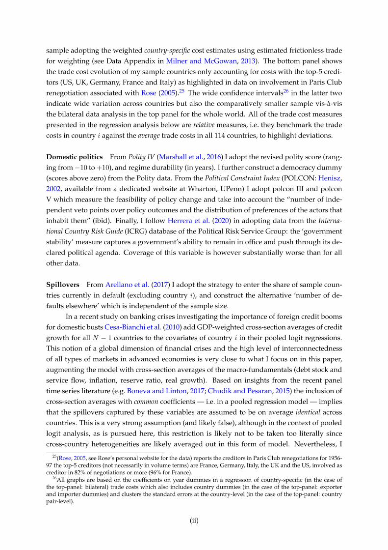
3.1 Sample

My sample covers up to 114 developing economies for the period 1970-2015 (raw data prior

to variable transformations; unbalanced panel). These economies experienced 174 debt crises,

but due to data coverage for other variables the regression samples only capture at most 171 of

these — for the same reason the empirical analysis is conducted for a sample of 102 countries

which experienced 141 crises. Details on sample makeup and descriptive statistics are relegated

to an Appendix. Figure 1 gives an idea of the distribution of crisis events and the distinction

between S&P-defined default and large IMF financing (in the upper panel), as well as of the

share of sample countries in default (left axis) along with the sample evolution over time (in

the lower panel) — in both cases I highlight the differences between the S&P definition of

default and that of large official financing.

Figure 2 gives some insights into the evolution of median debt stocks (official, private)

and debt service flows (relative to GNI) over time. Official debt stock (solid blue line, right

scale) appears hump-shaped with a maximum in the early eighties, though followed by a per-

sistently high level for a period of almost 20 years. From 2007 onwards levels of official debt

were substantially reduced to pre-1978 oil crisis magnitudes (G8 multilateral debt relief initia-

tive in 2005), and have remained relatively stable since. Debt stocks from private lenders (yel-

10

low line) are most significant in the late 1970s/early 1980s, and have recently made a comeback.

The median of debt service flows (dashed black line, left scale) largely shares the evolution of

the official debt stock, though it has a more pronounced early peak in 1988 and a second, albeit

much lower, peak in the early noughties.

3.2 Variable Construction

In the following I describe the dependent and independent variables in broad brushes — a

detailed discussion of variable construction and sources is contained in Appendix A. Appendix

Figure D-1 shows the results of an event analysis study for a number of candidate predictors

of sovereign default.

My dependent variable is an indicator for the first year of default, adopting the Standard

& Poor’s definition of a credit event (about 1/3 of events, largely taken from Reinhart and

Rogoff, 2009) and/or that of exceptionally large financing from the IMF (Medas et al., 2018).10

I construct the reputation proxies based on the memory variables in Catão and Mano

(2017): the rolling share of years spent in default, using 1950 as a starting point (bad reputation);

and the rolling count of years since the last default (also, variations with different discounting).

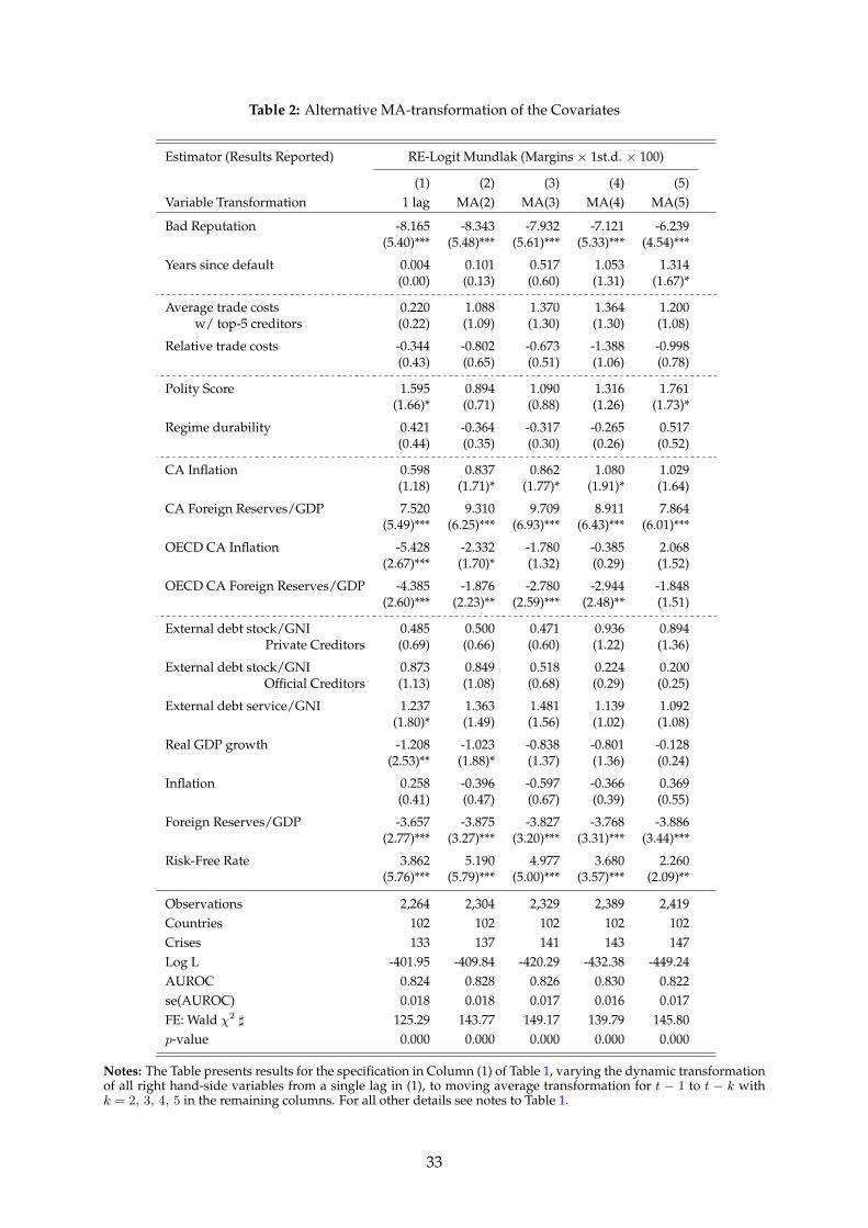
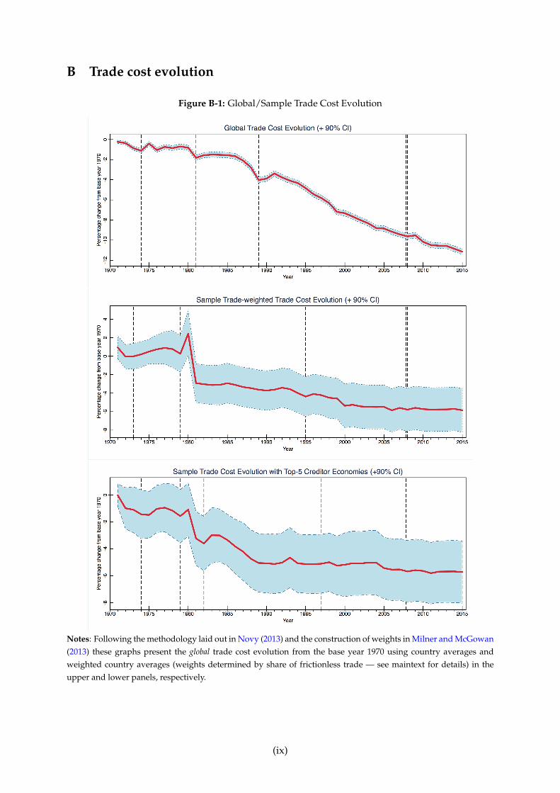
The direct punishment variables are intended to capture the exposure of sovereigns to

the potential for trade sanctions (whether explicit or implicit) and with this the incentives for

sovereigns to avoid or defer default.11 I hypothesise that lower membership in formal trade

networks (especially those of economic significance as evidenced by actual trade flows) deters

sovereigns from entering into default. I construct RTA (regional trade agreements) counts and

trade-weighted RTA counts based on the Regional Trade Agreements Database (Egger and

Larch, 2008). I further hypothesize that a sovereign with higher trade costs will fear trade-

related reprisals and thus have incentives not to default. I compute trade costs following the

methodology introduced in Novy (2013) and Milner and McGowan (2013) using bilateral trade

data from IMF DOTS and GDP data from the World Bank WDI. One variant here is to focus on

trade costs with major creditors (France, the US, Germany, the UK, and Italy). All of the trade

cost measures are relative measures, i.e. they benchmark the trade costs in country i against the

average trade costs in all 114 countries, to highlight deviations.

Measures related to domestic politics are taken from Polity IV: the revised polity score

(ranging from −10 to +10), and regime durability (in years). I also construct a democracy

dummy for Polity IV scores above zero. From POLCON I use polcon III and polcon V which

measure the feasibility of policy change. Following Herrera et al. (2020) I adopt ‘government

10Following the standard in this literature (e.g. Catão and Milesi-Ferretti, 2014) the observations for countries indefault following the first crisis year are omitted.

11Trade of debtor countries is known to decline after default (Rose, 2005), especially so with debtor countries; inthe present dataset merchandise trade drops by around 1-2% following default.

11

stability’ from ICRG.

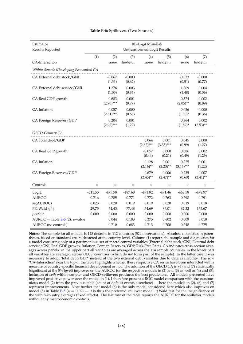
I pursue a number of strategies to capture international spillovers: following Arellano

et al. (2017) I construct the share of sample countries currently in default (excluding country i)

and the alternative ‘number of defaults elsewhere.’ Inspired by a recent study on banking crises

investigating the importance of foreign credit booms for domestic busts (Cesa-Bianchi et al., 2010)

I compute the cross-section averages of macro-fundamentals (debt stock and service flow, infla-

tion, reserve ratio, real growth) and include these alongside their country-specific versions. In

alternative specifications these cross-section averages are interacted with time-invariant (base

year) measures of trade openness (imports plus exports divided by GDP, taken from the WDI)

or financial development (proxied by bank credit to bank deposits from the World Bank Global

Financial Development Database (GFDD). The latter is motivated by the recent literature on ‘too

much finance’ and the potential trade-off between growth and crisis vulnerability. I provide

an econometric rationale for this setup in Section 4 below. I further construct these ‘spillover’

variables for OECD countries, which are not part of my sample, capturing the ‘core-periphery’

notion of Kaminsky and Vega-Garcia (2016).

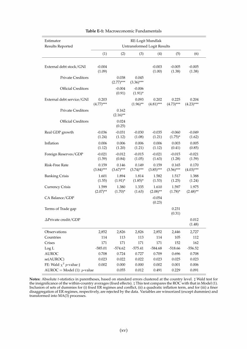
A great deal of other variables have been suggested in the existing literature. Measures

of debt stock and debt service flow are quite common, and I adopt the external debt to GNI

measures (stock, service flows) from GFDD — these are also available split into private and

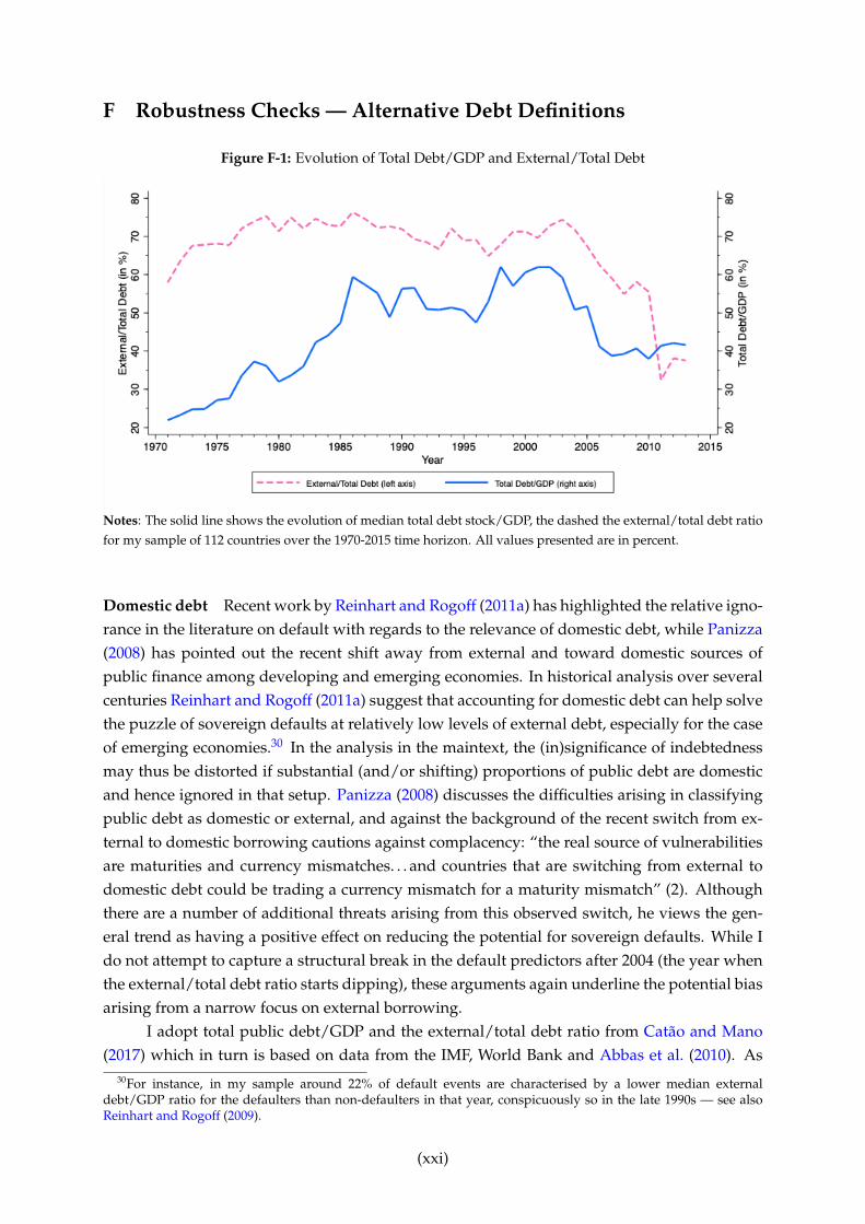
official creditors. In robustness checks I adopt total public debt and the external/total debt

ratio from Catão and Mano (2017) to follow up on the insights from recent work on domestic

debt (Panizza, 2008; Reinhart and Rogoff, 2011a); private and public debt from the 2018 GDD

(Mbaye et al., 2018); and the present-value external debt data from Dias et al. (2014).

Additional macroeconomic fundamentals include real GDP growth from the WDI, infla-

tion (I adopt the GDP deflator from WDI for improved coverage), the foreign reserves to GDP

ratio from Catão and Mano (2017) augmented with data from the WDI, the current account

balance as a measure of external balance and the terms of trade gap (all taken from the same

study). The 10-year US Treasury constant maturity rate to capture the state of the global eco-

nomic environment is taken from FRED. In robustness checks I use an update to the Chinn and

Ito (2006) capital account openness index (standardized), as well as country-specific commod-

ity price growth and volatility measures adopted from Eberhardt and Presbitero (2021); capital

flow bonanzas are constructed following Caballero (2016) using net capital inflows as a share

of GDP from the IMF Financial Flows Analytics database.

I use data from Ilzetzki et al. (2019) to classify countries with fixed exchange rate regimes

as well as a finer disaggregation. Dummy variables for banking and currency crises (start year)

come from a 2017 update to Laeven and Valencia (2013). From Marshall (2017) I take ‘major

episodes of political violence’ involving at least 500 deaths.

12

The above empirical measures treat the manifestation of each theoretical strand as sep-

arate from macroeconomic fundamentals. As the discussion in Panizza (2013) suggests, this

separation is clearly not always warranted, given that reputational motives, direct punish-

ment/incentives, domestic politics, and also spillovers affect the ‘choice’ and thus evolution of

the level of public indebtedness and foreign exchange reserves, among others: bad reputation

or punishment may prevent a country’s access to international financial markets, thus directly

affecting the public debt to GDP ratio. I try to capture these channels by interacting some of the

above ‘theory strand’ variables with the two most relevant macro fundamentals ‘controlled’ by

the domestic government: the external debt to GDP ratio and the foreign reserve ratio.

3.3 Variable Transformations

Outliers can at times drive empirical results, especially when analysing macro variables such as

inflation or indebtedness which cover a vast range of values. I therefore follow standard empir-

ical practice and wisorise the top and bottom one percent of observations for each continuous

variable, respectively.

One important aspect of the empirical modelling of default and more generally financial

crises is how to take account of the pre-crisis dynamics of macroeconomic variables in the con-

struction of an ‘early warning’ approach. In this context, the standard practice in the literature

is to lag the regressors, typically by just a single time period (e.g. Catão and Mano, 2017). This

choice seems somewhat ad hoc and may fail to adequately capture the prevailing dynamics in

the run-up of a crisis. In their seminal contribution on banking crises Schularick and Taylor

(2012) employ lag polynomials of length five in their analysis of advanced economies over a

140-year time period. Given the comparatively short time series dimension of my panel data

(on average 23 years) along with the large number of candidate determinants included in the

model, I adopt moving averages to capture pre-crisis dynamics, as practiced by Reinhart and

Rogoff (2011b) and Jordà et al. (2011, 2016) — based on the below event analysis I select an

MA(3) process, for t − 1 to t − 3. I further present results for a single lag as well as MA(2) to

MA(5) transformations for robustness.

4 Empirical Model and Implementation

I follow the majority of studies in the financial crisis literature and estimate a latent crisis model,

where the observed variable (the debt crisis) is a realized event when the latent variable exceeds

some threshold. I code the crisis variable as equal to one in the year the debt crisis starts, and

zero otherwise.

A key issue to confront in order to obtain robust estimates is unobserved cross-country

13

heterogeneity. I adopt an empirical implementation which deals with this issue by allowing

for country-specific fixed effects, which give all coefficients the interpretation of ‘within’ coun-

try estimates and thus come closer to a plausibly causal interpretation of the results, but at

the same time are not subject to the incidental parameter problem. One disadvantage of the

standard practice in the literature, where fixed effects are simply included in a pooled logit

or probit model (e.g. Gelos et al., 2011; Catão and Milesi-Ferretti, 2014), is that the regression

sample is limited to those countries which experienced a crisis at one point during the sample

period. Since this implementation excludes countries which avoided crises it may run the risk

of distorting the results due to a sample selection effect.12

To overcome this limitation, I follow the practice in Caballero (2016), who adopts a well-

established empirical approach to get around the incidental parameter problem in nonlinear

models, dating back to Mundlak (1978) and a generalisation by Chamberlain (1982). The im-

plementation (henceforth RE-Mundlak Logit) builds on a random effects logit model, where

the strong assumption of no correlation between the individual (in my case country-specific)

effects and the covariates can be relaxed by separately including the country-specific means of

each variable. Further, the statistical significance of accounting for country-specific effects can

easily be tested. The empirical setup is based on a binary choice model:

Y ∗it = α′idt + β

′Xit + eit, (1)

where Y ∗it is a latent variable relating to the observed response variable, Yit (the default start

year), via the indicator function Yit=1(Y ∗it ). Thus Yit = 1 if Y ∗it > 0 and zero otherwise. dt may

include observed common factors and country fixed effects (when dt = 1∀t).

The estimated model simply adds the within-country averages of all time-varying vari-

ables, X̃ , to the random effects logit model to capture the between-country variability in the

propensity of default, which can be argued to arise from factors related to (colonial) history, ge-

ographic location and relatedly natural resource environment, as well as legal system and other

determinants. If the true model does contain such individual effects and these are correlated

with the other covariates in the model, the resulting coefficients of interest β̂ are asymptotically

biased if these ‘fixed effects’ are ignored by the econometrician. Standard errors are clustered at

the country-level in the raw logit regressions, and computed from these via the Delta method

in the marginal effects.

The inclusion of cross-section averages in the empirical model (following Cesa-Bianchi

et al., 2010) to capture spillovers can be given a more formal justification from the macro panel

12In Appendix H I present the results for such a specification (logit with country fixed effects). Estimated marginaleffects follow quite similar patterns of signs and statistical significance, although coefficient estimates are typicallyinflated whle external debt plays a greater role in these specifications.

14

econometric literature. A recent contribution by Boneva and Linton (2017) adopts the common

factor error structure from the linear macro panel literature (see Chudik and Pesaran, 2015, for

a detailed survey) and extends this concept to the nonlinear panel setup. With reference to

equation (1) above they specify:

eit = λ′ift + εit, (2)

where f is a set of unobserved common factors, the λi are associated unknown factor loadings

and ε is white noise. These factors are further assumed correlated with the independent vari-

ables Xit in (1), such that their omission induces omitted variable bias in the estimates of β.

A widely-cited paper by Pesaran (2006) establishes for the linear model that the unobserved

common factors can be proxied by the inclusion of the cross-section averages of all dependent

and independent variables, while the country-specific factor loadings are captured by estimat-

ing the model separately for each country, or by interacting each cross-section average with N

country dummies (see Eberhardt and Presbitero, 2015, for a recent empirical application). The

contribution by Boneva and Linton (2017) establishes that this idea extends to nonlinear models

where the cross-section averages are based only on the independent variables, and where the

model in (1) augmented with cross-section averages is estimated separately for each country.

This ‘common correlated effects’ estimator is however not feasible in the present panel of

relatively modest time series dimension. The elaborate econometric excursion above can how-

ever give some insights into the assumptions made (and relaxed) when cross-section averages

(CA) are included in a pooled logit model as is suggested here: if the CA are simply added

to the model, we are implicitly assuming that the factor loadings are identical across countries,

hence eit = λ′ft+εit. This is a strong assumption. Since the λi parameters cannot be freely esti-

mated in my model I experiment with two forms of country-specific spillover variables by inter-

acting the cross-section averages with time-invariant measures for trade openness and financial

development, respectively.13 These interactions relax the assumption that λi = λ and mimic

the country-specific nature of the factor loadings with country-specific values: eit = λ∗i′ft+ εit.

At the same time they restrict the ‘spillover channels’ to be proxied by a country’s openness to

trade or level of financial development.

Finally, in my empirical analysis I use the Receiver Operating Characteristic (ROC) curve

along with the associated AUROC (area under the ROC curve) statistic, which has become a

prominent feature of the empirical literature on financial crises (see Jordà et al., 2011; Schular-

ick and Taylor, 2012), to study the predictive power of the model. A higher AUROC statistic

(bounded between 0 and 1) indicates better predictive power (a value of 0.5 represents the

13This is motivated by existing work on crisis propagation and international spillovers (Glick and Rose, 1999;Van Rijckeghem and Weder, 2001). I use country-specific averages for openness and findev as weights followingCiccone (2018).

15

benchmark for any informative model, where predictive power is equivalent to the flip of a

coin), and statistical tests to compare the predictive power of different models can be con-

structed given the availability of AUROC standard errors.

5 Results and Discussion

5.1 Results by Theory Strand

The results for separate regressions by theory strand are discussed in details in an Appendix

section. In all cases candidate variables for each strand are tested for predictive power in a

benchmark model of macro-economic determinants of default. The selection of the latter is

also discussed in the Appendix.

5.2 Main Results

In Table 1 I bring together results from models including the empirical interpretations of the

four theory strands alongside macroeconomic fundamentals. The estimates presented in this

table are marginal effects, which I have multiplied by one hundred times the standard devi-

ation of the covariate in question — for ease of discussion I will refer to these as ‘marginal

effects’. Column (1) presents the benchmark specification, all other models are tested against

this specification in terms of their predictive power: the final row of the table presents p-values

for the statistical comparison between the benchmark in (1) and each other model. Models (2)

and (3) provide results for alternative spillover proxies, where the former represents a single

variable (count of default events elsewhere), whereas the latter is a more elaborate specifica-

tion — there is the potential that the cross-section averages may pick up the impact of other

omitted variables, such that we can think of the results for the default count in (2) as the lower

bound and those for the CA specifications in (1) and (3) as the upper bound of the spillover ef-

fects. The remaining four models each drop one of the theory strands for comparison with the

benchmark results.14 Note that for all results presented in this and the following section, model

comparison tests (ROC comparison) always rejected the joint omission of all theory strands or

of all macro-fundamental variables.

Reputation acts as a disciplining device: having a higher share of years in default since

1950 (‘Bad Reputation’) and/or a more recent history of default are associated with lower de-

fault rates — the latter result is only significant in the parsimonious spillover specification in

(2) or when spillovers are excluded in (7). The trade cost measures are statistically insignificant

14If this exercise in (4)-(7) is repeated with the parsimonious model in (2) — see Appendix Table G-1 — therelative magnitude of spillover versus reputation coefficients is similar, and the ROC comparison indicates thesame patterns of significance for the reputation, politics, and spillover theory strands.

16

throughout except when spillovers are excluded in (7). A higher Polity IV score is associ-

ated with higher default propensity, but this measure is only significant in the parsimonious

spillover specification in (2) and again when spillovers are excluded, while regime durability

flips signs across the three spillover specifications and is never statistically significant. As is

already clear from the above, the specification of the spillover variable(s) has significant bear-

ings on the results for all other covariates: the benchmark model in (1) particularly highlights

the role for foreign reserves elswhere for domestic default, both in sample countries and the

OECD, which is also reflected in the results for the more elaborate model in (3) — the effects

of all spillover variables are in addition to the global economic climate captured by the risk free

rate, which in turn is highly significant and positive in the benchmark model but not in the two

alternatives. Notable among the macro fundamentals are the strong significant associations

of the reserve ratio (negative — the opposite sign to the sample spillover variable) as well as

the insignificance of GDP growth, inflation and debt stock effects (except when spillovers are

excluded), respectively. Debt service flows, in support of the notion expressed in Sturzenegger

and Zettelmeyer (2007) that debt payments rather than stock enter into a sovereign’s considera-

tion, have a positive association with default though this is only statistically significant in the

parsimonious spillover model in (2).

The signs of these measures in either models (1) or (2)15 are in line with the raw logit

estimates from the separate strand regressions discussed in Appendix E. The marginal effects

computed and presented allow for direct comparison of the economic magnitudes of the effects

across strands and measures. Quantitatively the largest effects are associated with ‘bad repu-

tation’ and spillover effects, depending on the specification choice for the spillovers. As was

suggested above, if we worry about the conflation of spillovers and omitted variables in the

results for the various cross-section averages, then the parsimonious ‘default count’ specifica-

tion in (2) can perhaps provide a narrower definition of spillover effects, which still highlights

the economic significance of this theory strand. Among the macro-fundamentals the global

economic environment (risk-free rate) and the foreign reserve ratio have the highest economic

significance, with debt service somewhat more moderate in effect.

The remainder of the table presents two sets of statistics alongside empirical results

testing the robustness of the benchmark model in (1), while Table G-1 in the Appendix does

the same for the model in (2): the final table row compares the predictive power with re-

stricted models where in (4)-(7) the set of variables associated with each theory are dropped,

respectively (see ‘Theory omitted’ near the top of the table for orientation). In all but the

threat/incentive case in (5) these restricted models are rejected by this measure of empirical

15It is somewhat academic to discuss consistency of signs between various models when coefficients are estimatedimprecisely such as the domestic politics proxies.

17

fit, implying that the omitted theory ‘matters’ in terms of predictive power. Investigating the

joint (in)significance for each strands of covariates (row marked ‘Theory’ toward the bottom

of the table) indicates that the threat/incentive and domestic politics measures are statistically

insignificant (p = .42 and p = .58) — these tests were carried out for the benchmark model in

(1). Country fixed effects (implemented via time-series averages) are significant in all models

presented, vindicating the choice of the RE-Mundlak approach over a logit fixed effects model.

In addition to the specifications presented a number of alternative or additional measures

were considered for each theory strand (detailed results available on request), which resulted

in identical or inferior predictive power and statistically insignificant coefficients, so that these

covariates were dropped/dismissed in favour of those presented.16 Similarly, the patterns of

my results are qualitatively unchanged (all results are available on request) when I (i) include

the first difference of the Chinn and Ito (2006) standardized measure for capital account open-

ness (2017 update) or run a split sample regression by level of capital account openness, to

gauge the effect of levels or changes in capital controls (Bai and Zhang, 2012);17 (ii) include

the annual growth of an aggregate index for primary commodity price movements along with

its 12-month rolling standard deviation (see Eberhardt and Presbitero, 2021);18 (iii) exclude the

full time series, post-decision point observations or decision-point to completion date obser-

vations in the 34 countries in my sample considered for the Highly Indebted Poor Countries

(HIPC) initiative of debt relief (Cassimon et al., 2015); I also estimate a split-sample regression

for non-HIPC and HIPC countries;19 (iv) include a squared term for inflation in an effort to

capture the hyper-inflation-default nexus of Reinhart and Rogoff (2011b);20 (v) add in controls

16None of the following alternatives changed/improved the predictive power of the benchmark results: expon-tentially discounted years since default (statistically significant at the 1% level), the addition of trade-weightedRTA counts (insignificant), measures of political constraints (insignificant), interactions between trade opennessor financial development and the cross-section averages of inflation and reserves (mixed significance), additionalcross-section averages for real growth, debt stock or service flows (insignificant).

17Following their cautious endorsement by the IMF in certain circumstances, the merits and perils of capitalcontrols in emerging economies are currently subject to debate (Montecino, 2018). In my sample the inclusion of thechange in the Chinn-Ito index of capital account openness leads to a negative significant coefficient on this variable,but no improvement in predictive power (p = .57). A 1 sd change in capital account openness is associated witha 0.85% decline in default propensity — this is a modest effect compared with that associated with reputation orspillover effects and other macro fundamentals. The split sample regressions yield similar patterns across theorystrands as the pooled analysis, though forex/GDP spillovers and the risk-free rate have statistically significantlylarger effects in economies with more capital constraints.

18The commodity price growth and volatility terms have the expected signs but only the latter is statisticallysignificant in a reduced sample from 1981-2015 (114 defaults in 99 countries), in line with the findings in Eberhardtand Presbitero (2021). The exclusion of the 1970s reduces the magnitudes of the spillover variables in the benchmarkmodel without commodity prices; upon their inclusion the relative magnitudes of reputation, punishment, politics,spillover, and macro-fundamentals remain qualitatively identical.

19Note that other debt relief initiatives, such as the Baker and Brady plans studied in Reinhart and Trebesch (2016),were dealing with countries debt restructing following default. Since I exclude ongoing crisis years these policyinterventions do not come to bear on the prediction of (future) crises in these countries. Relative magnitudes ofthe theory strand proxies and macro-fundamentals are qualitatively unchanged in the reduced sample regressions.In the split sample regression the economic magnitudes are larger in the HIPC sample though only statisticallysignificantly so for the spillover variables, the debt stocks and the risk-free rate. Patterns across theory strands areagain very similar to those reported above.

20The coefficient on the squared term has the expected positive sign but neither term is statistically significant.

18

for capital inflow bonanzas (Caballero, 2016) and ‘double bonanzas’ (Reinhart et al., 2016).21

and (vi) exclude ‘new sovereigns’ emerging from the breakup of the Soviet Union during the

early 1990s.

Additional analysis employs alternative measures for sovereign debt from Catão and

Mano (2017) for domestic debt, Dias et al. (2014) for external debt in net present value, and

Mbaye et al. (2018) for private debt. These results are presented in Appendix F and confirm the

general patterns of statistical significance and effect magnitude in the main analysis.

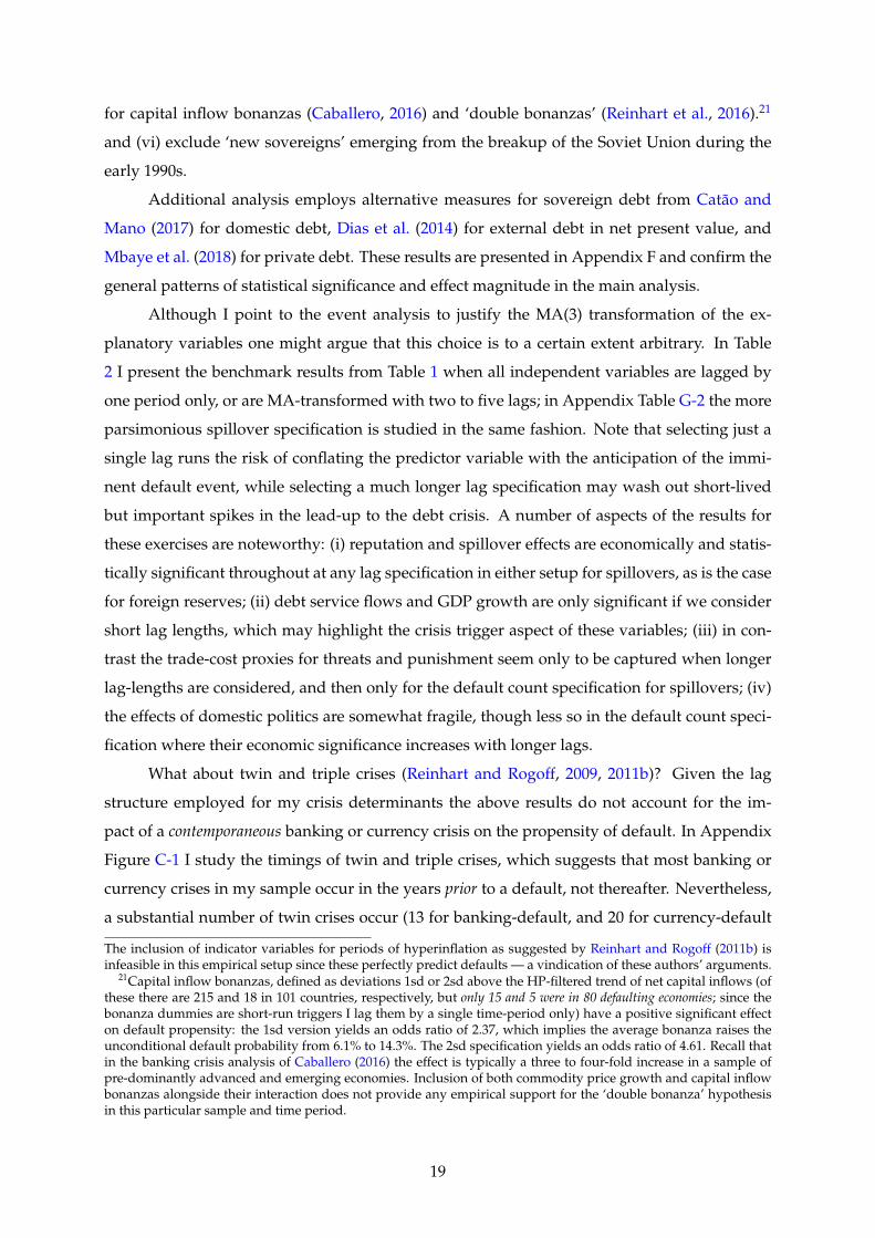
Although I point to the event analysis to justify the MA(3) transformation of the ex-

planatory variables one might argue that this choice is to a certain extent arbitrary. In Table

2 I present the benchmark results from Table 1 when all independent variables are lagged by

one period only, or are MA-transformed with two to five lags; in Appendix Table G-2 the more

parsimonious spillover specification is studied in the same fashion. Note that selecting just a

single lag runs the risk of conflating the predictor variable with the anticipation of the immi-

nent default event, while selecting a much longer lag specification may wash out short-lived

but important spikes in the lead-up to the debt crisis. A number of aspects of the results for

these exercises are noteworthy: (i) reputation and spillover effects are economically and statis-

tically significant throughout at any lag specification in either setup for spillovers, as is the case

for foreign reserves; (ii) debt service flows and GDP growth are only significant if we consider

short lag lengths, which may highlight the crisis trigger aspect of these variables; (iii) in con-

trast the trade-cost proxies for threats and punishment seem only to be captured when longer

lag-lengths are considered, and then only for the default count specification for spillovers; (iv)

the effects of domestic politics are somewhat fragile, though less so in the default count speci-

fication where their economic significance increases with longer lags.

What about twin and triple crises (Reinhart and Rogoff, 2009, 2011b)? Given the lag

structure employed for my crisis determinants the above results do not account for the im-

pact of a contemporaneous banking or currency crisis on the propensity of default. In Appendix

Figure C-1 I study the timings of twin and triple crises, which suggests that most banking or

currency crises in my sample occur in the years prior to a default, not thereafter. Nevertheless,

a substantial number of twin crises occur (13 for banking-default, and 20 for currency-default

The inclusion of indicator variables for periods of hyperinflation as suggested by Reinhart and Rogoff (2011b) isinfeasible in this empirical setup since these perfectly predict defaults — a vindication of these authors’ arguments.

21Capital inflow bonanzas, defined as deviations 1sd or 2sd above the HP-filtered trend of net capital inflows (ofthese there are 215 and 18 in 101 countries, respectively, but only 15 and 5 were in 80 defaulting economies; since thebonanza dummies are short-run triggers I lag them by a single time-period only) have a positive significant effecton default propensity: the 1sd version yields an odds ratio of 2.37, which implies the average bonanza raises theunconditional default probability from 6.1% to 14.3%. The 2sd specification yields an odds ratio of 4.61. Recall thatin the banking crisis analysis of Caballero (2016) the effect is typically a three to four-fold increase in a sample ofpre-dominantly advanced and emerging economies. Inclusion of both commodity price growth and capital inflowbonanzas alongside their interaction does not provide any empirical support for the ‘double bonanza’ hypothesisin this particular sample and time period.

19

events) and are therefore not captured by my analysis. In a robustness check I include dum-

mies for contemporaneous banking and currency crises in addition to the MA-transformed crisis

dummies (results available on request). Although both these dummies are positive significant

their inclusion does not lead to an increase in predictive power.22 The patterns of economic

magnitudes for the various theory strands and macro-fundamentals described above also do

not change in any substantial way.

A qualitative conclusion from this analysis is that there is empirical evidence for the

significance of all but the direct punishment theory for sovereign default, while it appears that

reputation and spillover effects trump all other factors in terms of economic significance. While

there is some tentative evidence for domestic politics affecting default, the direct punishment

strand produces no statistically significant results and fails to increase the predictive power of

the model. Foreign reserves, debt service and the global economic environment (risk-free rate)

are additional macro controls which statistically significantly affect the default propensity.

5.3 Extension: Heterogeneities across Countries and over Time

Thus far the analysis has treated hypothesised crisis determinants as covariates. This section

presents a number of extensions to the above preferred specification, intended to speak to the

concern that different ‘types’ of countries, where type is defined by political regime, ER regime,

etc., are characterised by entirely different default determinants. In each case I devise a sample

split which maintains both a substantial number of observations and defaults in each of the two

subsamples. Based on kmeans clustering of time-series averages of each country — meaning

countries cannot change clusters with the exception of the democracy/autocracy split where

failure of model convergence forced me to adopt a classification based on the time-varying

Polity IV score, and, naturally, the temporal split into early and late periods — I investigate

whether empirical results are significantly different (i) between democracies and autocracies,

(ii) between countries with fixed and flexible exchange rate regimes (based on the classification

in Ilzetzki et al., 2019), (iii) between countries with high and low financial development (using

private bank credit to deposits as a proxy), and (iv) over time (taking 1999 as the cut-off year).

In each case I add additional terms for all model variables interacted with a cluster dummy to

the benchmark specification in column (1) of Table 1.

Table 3 presents the pooled benchmark results (‘marginal effects’ defined as above) along-

side the models for sample splits as indicated. The shaded coefficient pairs rejected a simple

Wald test for equality in the underlying RE-Mundlak logit regression, where darker shading

indicates rejection at the 10% level, and lighter shading at the 15% level. Since sample splits

22Using again odds ratios to express the coefficient magnitudes on these contemporaneous terms suggests 2.9 forbanking and 3.16 for currency crises.

20

essentially double the number of parameters estimated it is not surprising that (a) the predic-

tive fit is, with one exception, better than for the pooled model (see ROC comparison in final

table row), and (b) many covariate coefficients are estimated much less precisely. The number

of default events in each cluster group is not necessarily the same or even close to the same,

while the number of parameters to estimate push the estimator to the limits of its feasibility.

With these caveats in mind I limit the discussion to two broad confirmations and a num-

ber of novel insights. First, regarding the former, across all sample splits (with the exception

of the temporal one) the marginal effects for bad reputation and the foreign reserves spillover

variables consistently have the same sign and in terms of economic magnitudes are signifi-

cantly larger compared with the marginal effects for any macro-fundamentals or alternative

theory strand proxies. Second, the trade cost proxies for the direct punishment theory strand

are insignificant throughout, and of the domestic politics proxies only regime durability shows

some signs of significance (in statistical and economic terms). The first novel insight relates

to the differential significance of spillovers, which in line with network arguments appears to

be higher in economic terms in more financially integrated economies. These economies are

much more susceptible to default if they have high debt services, but they can also reduce

default risk via a growth spurt, a tool which is not available to countries with low levels of fi-

nancial development. Second, the effect of reputational proxies varies substantially over time,

with the negative effect of a bad reputation massively larger in the more recent period, and the

memory effect (years since default) fading into insignificance in this period as well.23 Third,

countries with more flexible exchange rates differ significantly in the effects of their macro-

fundamentals from countries with fixed ER regimes: debt stock and service flows have more

substantial effects on default propensity, same goes for inflation, though GDP growth has a

stronger moderating effect. Although the moderating effect of foreign reserves is economically

significant in the flexible ER economies, this pales against the safeguard provided by reserves

in fixed ER regimes. Fourth, there is very little evidence for a ‘democratic advantage’ if this is

interpreted as differential effects for democracies versus autocracies, with the impact of bank-

ing crises the sole covariate significantly different across political regimes. Finally, the spillover

variables provide some very stark coefficient magnitudes for the foreign reserve cross-section

averages in the more recent time period, suggesting that perhaps the significance of this theory

strand has increased vis-à-vis the earlier period.

These novel insights aside the sample split exercise primarily serves to confirm the pat-

terns of statistical significance and economic magnitudes concluded from the pooled analysis

23With reference to the graphs in Figure 1 this pattern may be explained by the relative absence of defaultsfollowing the S&P definition from the turn of the century: 82% of defaults in this period were due to exceptionalylarge official financing, whereas during 1970-1999 this type made up only 60% of defaults. 83% of defaults followingthe S&P definition were before 2000.

21

in Table 1. The conistency of major factors across specifications as described is a very strong

indication of the pervasiveness and robustness of reputation, spillover and macro-fundamental

effects on sovereign default.

6 Concluding remarks

This paper asked which factors dominate statistically and economically in predicting sovereign

default events in developing and emerging economies over the past forty years. Standard

approaches in economics have traditionally emphasised either reputational concerns or the

threat of punishment, while a more recent literature has modelled international finance as a

global network which sovereign borrowers either exploit strategically or which subjects them

to higher default risk due to spillovers and ‘cascades of failures’. Much of the political science

literature in contrast has focused on the role of political regime and domestic politics with less

concern for punishment and reputation (Michael Tomz being a notable exception).

In this paper I provide a wide range of empirical proxies for the four primary theoret-

ical strands alongside standard macroeconomic controls. These proxies come in the form of

constructed variables, but additional interactions with macro fundamentals and sample splits

by political regime or exchange rate arrangement among others can cover a wide range of

theoretical prescriptions on the possible manifestation of or channel of impact for reputation,

punishment, political, and spillover effects.

The main contribution of this paper is the pursuit of an empirical early warning system

approach including all four main theory strands, which in the existing literature are analysed

separately. This analysis yields a number of novel and important insights: first, reputational

and international spillover effects quantitively play the most significant role in predicting de-

fault events in a large sample of developing and emerging economies. Second, sound empirical

evidence for the significance of direct punishment is less forthcoming, while the impact of do-

mestic politics is fragile and comparatively modest in economic terms. Third, foreign reserves

consistently provide moderating effects on default propensity which in economic terms are

large though not necessarily on par with the reputation and spillover effects. Fourth, these

findings are qualitatively robust to (i) sample splits by a variety of measures including ER ar-

rangements and political regime, (ii) the use of alternative definitions for public debt as well as

the consideration of private debt, (iii) alternative variable transformations to capture pre-crisis

dynamics, as well as (iv) a host of additional covariates related to commodity price movements,

hyper-inflation, or capital controls.

While this study focused on sovereign default in developing and emerging economies

the economic environment in the world at large is captured in at least two ways: first, by the

22

inclusion of the risk-free rate, and second, by the inclusion of cross-section averages for macro

fundamentals in OECD countries.

An empirical study of a comparatively small number of default events (6% of observa-

tions) with a large number of candidate predictors is always subject to concerns over a range

of technical issues, starting from overfitting bias,24 to empirical conflation of theoretically sep-

arate phenomena, to technically insurmountable problems such as constructing meaningful

marginal effects for interaction effects in nonlinear models, to overinterpretation of results for

flawed proxies to theoretical concepts. It was for instance not possible here to disentangle

strategic behaviour from inevitable ‘fate’ in the analysis of international spillovers; many nu-

ances of ongoing theoretical work on the reputation and direct punishment channels also had

to be ignored, while the difficulty of modelling unobserved threats and incentives may have

contributed to the failure to elucidate any significant effects for the punishment theory strand;

and finally, while the split into early and late time periods yielded some stark differences and

thus indicative evidence, the cross-country empirical approach applied here is not best-suited

to speak to the dramatic changes seen in, for instance, the shift from external to domestic debt

or the rise of private debt among developing countries over the past decade.

While all of these caveats and shortcomings must not be ignored, they cannot detract

from the economic significance of international spillovers, to date not widely recognised in the

sovereign default literature, and the confirmation of substantial reputation effects established

in this study.

24Stripped-down models of just individual proxies for each theoretical strand yield encouraging results for theanalysis of reputation and spillovers, and somewhat less enthusiastic support for punishment and domestic politics.

23

References

Abbas, S. A., Belhocine, N., El Ganainy, A., and Horton, M. (2010). A historical public debt

database. IMF Working Paper WP/10/245.

Acemoglu, D., Ozdaglar, A., and Tahbaz-Salehi, A. (2015). Systemic risk and stability in finan-

cial networks. American Economic Review, 105(2):564–608.

Alfaro, L. and Kanczuk, F. (2005). Sovereign debt as a contingent claim: a quantitative ap-

proach. Journal of International Economics, 65(2):297–314.

Archer, C. C., Biglaiser, G., and DeRouen Jr, K. (2007). Sovereign bond ratings and democracy:

The effects of regime type in the developing world. International Organization, 61(2):341–365.

Arellano, C., Bai, Y., and Lizarazo, S. (2017). Sovereign risk contagion. National Bureau of

Economic Research, NBER Working Paper 24031.

Arellano, C. and Kocherlakota, N. R. (2008). Internal debt crises and sovereign defaults. Na-

tional Bureau of Economic Research, NBER Working Paper 13794.

Bai, Y. and Zhang, J. (2012). Financial integration and international risk sharing. Journal of

International Economics, 86(1):17–32.

Bassanetti, A., Cottarelli, C., and Presbitero, A. F. (2019). Lost and found: Market access and

public debt dynamics. Oxford Economic Papers, 71(2):445–471.

Beaulieu, E., Cox, G. W., and Saiegh, S. (2012). Sovereign debt and regime type: Reconsidering

the democratic advantage. International Organization, 66(4):709–738.

Benczúr, P. and Ilut, C. L. (2016). Evidence for relational contracts in sovereign bank lending.

Journal of the European Economic Association, 14(2):375–404.

Boneva, L. and Linton, O. (2017). A discrete-choice model for large heterogeneous panels with

interactive fixed effects with an application to the determinants of corporate bond issuance.

Journal of Applied Econometrics, 32(7):1226–1243.

Borensztein, E. and Panizza, U. (2009). The costs of sovereign default. IMF Staff Papers,

56(4):683–741.

Boz, E. (2011). Sovereign default, private sector creditors, and the IFIs. Journal of International

Economics, 83(1):70–82.

Bulow, J. and Rogoff, K. (1988). Sovereign Debt: Is To Forgive To Forget? American Economic

Review, 79(1):43–50.

24

Bulow, J. and Rogoff, K. (1989). A constant recontracting model of sovereign debt. Journal of

Political Economy, 97(1):155–178.

Bulow, J. and Rogoff, K. (2015). Why sovereigns repay debts to external creditors and why it

matters. VoxEU column, June 10, 2015; available at voxeu.org.

Caballero, J. A. (2016). Do Surges in International Capital Inflows Influence the Likelihood of

Banking Crises? Economic Journal, 126:281–316.

Cassimon, D., Essers, D., and Verbeke, K. (2015). What to do after the clean slate? Post-relief

public debt sustainability and management. Acropolis BeFinD Working Paper 3.

Catão, L. and Milesi-Ferretti, G. M. (2014). External liabilities and crises. Journal of International

Economics, 94:18–32.

Catão, L. A. and Mano, R. C. (2017). Default premium. Journal of International Economics, 107:91–

110.

Cesa-Bianchi, A., Martin, F. E., and Thwaites, G. (2010). Foreign Booms, Domestic Busts: The

Global Dimension of Banking Crises. Journal of Financial Intermediation, 39:58–74.

Chamberlain, G. (1982). Multivariate regression models for panel data. Journal of Econometrics,

18(1):5–46.

Chinn, M. D. and Ito, H. (2006). What matters for financial development? Capital controls,

institutions, and interactions. Journal of Development Economics, 81(1):163–192.

Chudik, A. and Pesaran, M. H. (2015). Large panel data models with cross-sectional depen-

dence: A survey. In Baltagi, B. H., editor, The Oxford Handbook on Panel Data, chapter 1.

Oxford University Press.

Ciccone, A. (2018). International commodity prices and civil war outbreak: New evidence for

Sub-Saharan Africa and beyond. CEPR Discussion Paper 12625.

Cole, H., Neuhann, D., and Ordonez, G. (2016). Debt crises: For whom the bell tolls. National

Bureau of Economic Research, NBER Working Paper 22330.

Dellas, H. and Niepelt, D. (2016). Sovereign debt with heterogeneous creditors. Journal of

International Economics, 99(S1):S16–S26.

Dias, D. A., Richmond, C., and Wright, M. L. (2014). The stock of external sovereign debt: Can

we take the data at ‘face value’? Journal of International Economics, 94(1):1–17.

25

Diaz-Alejandro, C. (1985). Good-bye financial repression, hello financial crash. Journal of De-

velopment Economics, 19(1-2):1–24.

Eaton, J. and Gersovitz, M. (1981). Debt with potential repudiation: Theoretical and empirical

analysis. Review of Economic Studies, 48(2):289–309.

Eberhardt, M. and Presbitero, A. F. (2015). Public debt and growth: Heterogeneity and non-

linearity. Journal of International Economics, 97(1):45–58.

Eberhardt, M. and Presbitero, A. F. (2021). Commodity prices and banking crises. Journal of

International Economics, forthcoming.

Egger, P. and Larch, M. (2008). Interdependent preferential trade agreement memberships: An

empirical analysis. Journal of International Economics, 76(2):384–399.

Eichengreen, B. and Portes, R. (1986). Debt and default in the 1930s: Causes and consequences.

European Economic Review, 30(3):599–640.

Elliott, M., Golub, B., and Jackson, M. O. (2014). Financial networks and contagion. American

Economic Review, 104(10):3115–3153.

Fuentes, M. and Saravia, D. (2010). Sovereign defaulters: Do international capital markets

punish them? Journal of Development Economics, 91(2):336–347.

Gelos, R. G., Sahay, R., and Sandleris, G. (2011). Sovereign borrowing by developing countries:

What determines market access? Journal of International Economics, 83(2):243–254.

Glick, R. and Rose, A. K. (1999). Contagion and trade: Why are currency crises regional? Journal

of international Money and Finance, 18(4):603–617.

Gruss, B. (2014). After the boom–commodity prices and economic growth in Latin America

and the Caribbean. IMF Working Paper 14/154.

Hatchondo, J. C. and Martinez, L. (2010). The politics of sovereign defaults. Federal Reserve

Bank of Richmond Economic Quarterly, 96(3):291–317.

Henisz, W. J. (2002). The institutional environment for infrastructure investment. Industrial and

Corporate Change, 11(2):355–389.

Herrera, H., Ordoñez, G., and Trebesch, C. (2020). Political booms, financial crises. Journal of

Political Economy, 128(2):507–543.

Ilzetzki, E., Reinhart, C. M., and Rogoff, K. S. (2019). Exchange arrangements entering the

twenty-first century: Which anchor will hold? The Quarterly Journal of Economics, 134(2):599–

646.

26

Jayachandran, S. and Kremer, M. (2006). Odious debt. American Economic Review, 96(1):82–92.

Jordà, Ò., Schularick, M., and Taylor, A. M. (2011). Financial Crises, Credit Booms, and External

Imbalances: 140 Years of Lessons. IMF Economic Review, 59(2):340–378.

Jordà, Ò., Schularick, M., and Taylor, A. M. (2016). Sovereigns versus banks: credit, crises, and

consequences. Journal of the European Economic Association, 14(1):45–79.

Kaminsky, G. L., Reinhart, C. M., and Vegh, C. A. (2003). The unholy trinity of financial conta-

gion. Journal of Economic Perspectives, 17(4):51–74.

Kaminsky, G. L. and Vega-Garcia, P. (2016). Systemic and idiosyncratic sovereign debt crises.

Journal of the European Economic Association, 14(1):80–114.

Laeven, L. and Valencia, F. (2013). Systemic banking crises database. IMF Economic Review,

61(2):225–270.

Levy-Yeyati, E. and Panizza, U. (2011). The elusive costs of sovereign defaults. Journal of

Development Economics, 94(1):95–105.

Manasse, P. and Roubini, N. (2009). Rules of thumb for sovereign debt crises. Journal of Inter-

national Economics, 78(2):192–205.

Marshall, M. G. (2017). Major Episodes of Political Violence, 1946-2016. Center for Systemic

Peace and Societal-Systems Research, http://www.systemicpeace.org/warlist/warlist.

htm, last accessed January 12, 2018.

Marshall, M. G., Gurr, T. R., and Jaggers, K. (2016). Polity IV Project: Political Regime Character-

istics and Transitions, 1800-2016. Center for Systemic Peace and Societal-Systems Research,

http://www.systemicpeace.org/polityproject.html, last accessed January 12, 2018.

Martinez, J. V. and Sandleris, G. (2011). Is it punishment? Sovereign defaults and the decline in

trade. Journal of International Money and Finance, 30(6):909–930.

Mbaye, S., Badia, M. M., and Chae, K. (2018). Global debt database: Methodology and sources.

IMF Working Paper WP/18/111.

Medas, P. A., Poghosyan, T., Xu, Y., Farah-Yacoub, J., and Gerling, K. (2018). Fiscal crises.

Journal of International Money and Finance, 88:191–207.

Milner, C. and McGowan, D. (2013). Trade costs and trade composition. Economic Inquiry,

51(3):1886–1902.

27

Mitchener, K. J. and Weidenmier, M. D. (2010). Supersanctions and sovereign debt repayment.

Journal of International Money and Finance, 29(1):19–36.

Montecino, J. A. (2018). Capital controls and the real exchange rate: Do controls promote

disequilibria? Journal of International Economics, 114:80–95.

Mundlak, Y. (1978). On the pooling of time series and cross section data. Econometrica, 46(1):69–

85.

North, D. C. and Weingast, B. R. (1989). Constitutions and commitment: the evolution of insti-

tutions governing public choice in seventeenth-century england. Journal of Economic History,

49(4):803–832.

Novy, D. (2013). Gravity redux: measuring international trade costs with panel data. Economic

Inquiry, 51(1):101–121.

Panizza, U. (2008). Domestic and external public debt in developing countries. UNCTAD

Discussion Paper No. 188.

Panizza, U. (2013). The politics of debt and debt crises. In Gnan, E., editor, The Interaction of

Political, Fiscal and Financial Stability: Lessons from the Crisis, chapter 6. SUERF: The European

Money and Finance Forum.

Pesaran, M. H. (2006). Estimation and inference in large heterogeneous panels with a multi-

factor error structure. Econometrica, 74(4):967–1012.

Reinhart, C. M., Reinhart, V. R., and Trebesch, C. (2016). Global Cycles: Capital Flows, Com-

modities, and Sovereign Defaults, 1815–2015. American Economic Review, Papers & Proceedings,

106(5):574–580.

Reinhart, C. M. and Rogoff, K. S. (2009). This Time is Different: Eight Centuries of Financial Folly.

Princeton University Press.

Reinhart, C. M. and Rogoff, K. S. (2011a). The forgotten history of domestic debt. The Economic

Journal, 121(552):319–350.

Reinhart, C. M. and Rogoff, K. S. (2011b). From financial crash to debt crisis. The American

Economic Review, 101(5):1676–1706.

Reinhart, C. M. and Trebesch, C. (2016). Sovereign debt relief and its aftermath. Journal of the

European Economic Association, 14(1):215–251.

Rose, A. K. (2005). One reason countries pay their debts: renegotiation and international trade.

Journal of Development Economics, 77(1):189–206.

28

Scholl, A. (2017). The dynamics of sovereign default risk and political turnover. Journal of

International Economics, 108:37–53.

Schularick, M. and Taylor, A. M. (2012). Credit booms gone bust: Monetary policy, leverage

cycles, and financial crises, 1870-2008. American Economic Review, 102(2):1029–61.

Schultz, K. A. and Weingast, B. R. (2003). The democratic advantage: institutional foundations

of financial power in international competition. International Organization, 57(1):3–42.

Shea, P. E. and Poast, P. (2018). War and default. Journal of Conflict Resolution, 62(9):1876–1904.

Sturzenegger, F. and Zettelmeyer, J. (2007). Debt defaults and lessons from a decade of crises. MIT

Press.

Tomz, M. (2002). Democratic default: Domestic audiences and compliance with international

agreements. Unpublished Mimeo, Stanford University.

Tomz, M. (2007). Reputation and International Cooperation: Sovereign Debt across Three Centuries.

Princeton University Press.

Tomz, M. and Wright, M. L. (2007). Do countries default in ‘bad times’? Journal of the European

Economic Association, 5(2-3):352–360.

Van Rijckeghem, C. and Weder, B. (2001). Sources of contagion: is it finance or trade? Journal of

international Economics, 54(2):293–308.

Van Rijckeghem, C. and Weder, B. (2009). Political institutions and debt crises. Public Choice,

138(3):387–408.

29

Figures and Tables

Figure 1: Default Event Frequency (top), Share of Sample in Default (bottom)

05

10

15

Co

un

t (u

nb

ala

nce

d p

an

el)

1970 1975 1980 1985 1990 1995 2000 2005 2010 2015Year

S&P Default Definition [61 events] Exceptionally Large Official Financing [113 events]

50

60

70

80

90

10

01

10

Co

un

trie

s in

th

e s

am

ple

0.1

.2.3

.4.5

Sh

are

of

sa

mp

le c

ou

ntr

ies in

de

fau

lt

1970 1975 1980 1985 1990 1995 2000 2005 2010 2015Year

Countries: In the sample (right scale) Share in default (left scale) Dto S&P definition only

Notes: N = 114. The sample covers the period 1970-2015; 88 countries experienced 174 default events (in theregression samples the maximum number of defaults covered is 171 due to data availability for the RHS variables).Both graphs report annual frequencies/values, the top graph highlights the difference between defaults defined byS&P and by exceptional official financing focusing on default start years, the bottom graph countries in default (alsoindicating the unbalancedness of the sample).

30

Figure 2: Evolution of External Debt/GNI (stock, service flow)

01

02

03

04

0E

xte

rna

l D

eb

t/G

NI

ratio

(in

%)

12

34

Exte

rna

l D

eb

t S

erv

ice

/GN

I ra

tio

(in

%)

1970 1975 1980 1985 1990 1995 2000 2005 2010 2015Year

Debt Service/GNI (left axis) Debt Stock/GNI by Lender (right axis): Private Official

Notes: The solid lines shows the median external public debt stock/GNI by lender (grey for private, black forofficial), the dashed line the median service/GNI ratio for my sample of 114 countries over the 1970-2015 timehorizon. All values presented are in percent.

31

Table 1: Main Results

Estimator (Results Reported) RE-Logit Mundlak (Margins × 1 st.d. × 100)

(1) (2) (3) (4) (5) (6) (7)Theory omitted Bad Rep Threats Politics Spillover

Bad Reputation -7.932 -4.783 -10.048 -8.089 -7.685 -3.280(5.61)*** (4.14)*** (5.19)*** (5.80)*** (4.72)*** (3.14)***

Years since default 0.517 1.522 0.120 0.558 0.680 2.576(0.60) (1.88)* (0.14) (0.67) (0.69) (3.14)***

Average trade costs -0.673 -0.542 -0.793 -0.917 -0.427 -0.746w/ top-5 creditors (0.51) (0.47) (0.58) (0.68) (0.28) (0.71)

Relative trade costs 1.370 1.395 1.261 1.723 1.494 2.086(1.30) (1.23) (1.08) (1.47) (1.25) (1.90)*

Polity Score 1.090 2.046 1.227 -0.051 1.176 2.563(0.88) (1.87)* (0.96) (0.04) (0.95) (2.23)**

Regime durability -0.317 0.640 -0.803 0.207 -0.191 0.902(0.30) (0.63) (0.77) (0.17) (0.19) (0.99)

CA Inflation 0.862 2.722 0.776 0.843 0.928(1.77)* (2.49)** (1.35) (1.73)* (1.82)*

CA Foreign Reserves/GDP 9.709 7.676 7.427 9.699 9.778(6.93)*** (2.46)** (5.53)*** (7.23)*** (5.89)***

CA External debt stock/GNI 1.084(0.29)

CA External debt service/GNI 4.260(1.35)

CA Real GDP growth 3.134(2.12)**

OECD CA Inflation -1.780 7.011 2.402 -1.854 -2.051(1.32) (3.14)*** (1.82)* (1.37) (1.44)

OECD CA Foreign Reserves/GDP -2.780 -2.027 -2.275 -2.856 -2.835(2.59)*** (1.40) (1.91)* (2.65)*** (2.46)**

OECD CA Total debt/GDP 8.513(2.11)**

OECD CA Real GDP growth -0.061(0.05)

Count of default 2.898events elsewhere (DC) (5.51)***

External debt stock/GNI 0.471 0.889 0.673 0.953 0.426 0.615 1.705Private Creditors (0.60) (1.21) (0.88) (1.20) (0.53) (0.68) (2.45)**

External debt stock/GNI 0.518 0.101 0.706 -0.983 0.651 0.480 -0.503Official Creditors (0.68) (0.13) (0.81) (1.28) (0.85) (0.51) (0.69)

External debt service/GNI 1.481 1.919 0.065 1.963 1.427 1.343 1.327(1.56) (2.18)** (0.07) (1.93)* (1.53) (1.34) (1.64)

Real GDP growth -0.838 -0.799 -0.765 -0.826 -0.790 -0.868 -0.837(1.37) (1.24) (1.18) (1.21) (1.28) (1.38) (1.29)

Inflation -0.597 0.340 -0.899 0.137 -0.420 -0.431 0.296(0.67) (0.38) (0.98) (0.16) (0.52) (0.46) (0.37)

Foreign Reserves/GDP -3.827 -3.271 -3.698 -3.657 -4.057 -3.678 -1.810(3.20)*** (2.98)*** (2.97)*** (2.25)** (3.13)*** (2.56)** (1.72)*

Risk-Free Rate 4.977 0.128 1.661 2.783 4.906 5.101 2.644(5.00)*** (0.15) (1.49) (2.96)*** (4.87)*** (4.54)*** (3.74)***

Standard errors Cluster Cluster Cluster Jack Cluster Jack ClusterLogL -420.29 -434.72 -403.21 -449.51 -421.65 -423.81 -451.43AUROC (se) 0.83 (.017) 0.81 (.019) 0.85 (.016) 0.79 (.019) 0.82 (.018) 0.82 (.018) 0.78 (.021)Theory: Wald χ2 p-value ‡ 0.000 0.418 0.576 0.000FE: Wald χ2 p-value ] 0.000 0.000 0.000 0.001 0.000 0.000 0.000AUROC = (1): p-value \ 0.137 0.004 0.002 0.150 0.042 0.002

Notes: All results are for 102 countries with 2,329 observations and 141 crises. The estimates presented are marginaleffects multiplied by 100 times the variable standard deviation. Banking and Currency crisis dummies included butnot reported. Absolute t-statistics in parentheses, based on standard errors computed via the Delta method (st.errorsfor RE-Mundlak logit clustered at country level; unless jackknife where indicated). Models (4)-(7) highlight thesignificance of each of the four theories. ] Wald test for the insignificance of the within-country averages. ‡ Thisindicates the joint significance of each ‘theory’ in model (1). \ This test compares the ROC with that of Model (1); in(4)-(7) rejection indicates that the benchmark model is preferred and that the theory variables omitted ‘matters’.

Table 2: Alternative MA-transformation of the Covariates

Estimator (Results Reported) RE-Logit Mundlak (Margins × 1st.d. × 100)

(1) (2) (3) (4) (5)Variable Transformation 1 lag MA(2) MA(3) MA(4) MA(5)

Bad Reputation -8.165 -8.343 -7.932 -7.121 -6.239(5.40)*** (5.48)*** (5.61)*** (5.33)*** (4.54)***

Years since default 0.004 0.101 0.517 1.053 1.314(0.00) (0.13) (0.60) (1.31) (1.67)*

Average trade costs 0.220 1.088 1.370 1.364 1.200w/ top-5 creditors (0.22) (1.09) (1.30) (1.30) (1.08)

Relative trade costs -0.344 -0.802 -0.673 -1.388 -0.998(0.43) (0.65) (0.51) (1.06) (0.78)

Polity Score 1.595 0.894 1.090 1.316 1.761(1.66)* (0.71) (0.88) (1.26) (1.73)*

Regime durability 0.421 -0.364 -0.317 -0.265 0.517(0.44) (0.35) (0.30) (0.26) (0.52)

CA Inflation 0.598 0.837 0.862 1.080 1.029(1.18) (1.71)* (1.77)* (1.91)* (1.64)

CA Foreign Reserves/GDP 7.520 9.310 9.709 8.911 7.864(5.49)*** (6.25)*** (6.93)*** (6.43)*** (6.01)***

OECD CA Inflation -5.428 -2.332 -1.780 -0.385 2.068(2.67)*** (1.70)* (1.32) (0.29) (1.52)

OECD CA Foreign Reserves/GDP -4.385 -1.876 -2.780 -2.944 -1.848(2.60)*** (2.23)** (2.59)*** (2.48)** (1.51)

External debt stock/GNI 0.485 0.500 0.471 0.936 0.894Private Creditors (0.69) (0.66) (0.60) (1.22) (1.36)

External debt stock/GNI 0.873 0.849 0.518 0.224 0.200Official Creditors (1.13) (1.08) (0.68) (0.29) (0.25)

External debt service/GNI 1.237 1.363 1.481 1.139 1.092(1.80)* (1.49) (1.56) (1.02) (1.08)

Real GDP growth -1.208 -1.023 -0.838 -0.801 -0.128(2.53)** (1.88)* (1.37) (1.36) (0.24)

Inflation 0.258 -0.396 -0.597 -0.366 0.369(0.41) (0.47) (0.67) (0.39) (0.55)

Foreign Reserves/GDP -3.657 -3.875 -3.827 -3.768 -3.886(2.77)*** (3.27)*** (3.20)*** (3.31)*** (3.44)***

Risk-Free Rate 3.862 5.190 4.977 3.680 2.260(5.76)*** (5.79)*** (5.00)*** (3.57)*** (2.09)**

Observations 2,264 2,304 2,329 2,389 2,419Countries 102 102 102 102 102Crises 133 137 141 143 147Log L -401.95 -409.84 -420.29 -432.38 -449.24AUROC 0.824 0.828 0.826 0.830 0.822se(AUROC) 0.018 0.018 0.017 0.016 0.017FE: Wald χ2 ] 125.29 143.77 149.17 139.79 145.80p-value 0.000 0.000 0.000 0.000 0.000

Notes: The Table presents results for the specification in Column (1) of Table 1, varying the dynamic transformationof all right hand-side variables from a single lag in (1), to moving average transformation for t − 1 to t − k withk = 2, 3, 4, 5 in the remaining columns. For all other details see notes to Table 1.

33

Table 3: Extensions — Sample Splits

Estimator RE-Logit Mundlak (Results reported: Cluster-Specific Margins × 1 st.d. × 100)

(1) (2) (3) (4) (5)Polity ER regime FinDev Time Period

Pooled Low High Fixed Flex Low High Early Late

Bad Reputation -7.932 -9.099 -7.921 -7.385 -11.243 -6.650 -13.782 -3.868 -18.117(5.61)*** (4.12)*** (3.00)*** (3.88)*** (4.59)*** (3.92)*** (3.03)*** (1.12) (5.83)***

Years since default 0.517 0.528 1.303 0.163 1.738 0.569 3.849 6.978 -0.833(0.60) (0.46) (0.59) (0.11) (1.31) (0.51) (2.19)** (2.20)** (0.68)

Average trade costs 1.370 1.452 1.760 0.291 0.678 1.361 0.032 -1.231 -0.308w/ top-5 creditors (1.30) (0.73) (1.23) (0.16) (0.40) (0.96) (0.01) (0.57) (0.09)

Relative trade costs -0.673 0.451 -1.460 0.799 -1.587 -1.574 0.724 -0.122 -0.379(0.51) (0.20) (1.17) (1.13) (0.68) (0.75) (0.47) (0.21) (0.11)

Polity Score 1.090 0.287 0.479 0.163 -1.360 0.165 3.251(0.88) (0.16) (0.24) (0.12) (0.37) (0.11) (1.11)

Regime durability -0.317 0.569 -0.983 1.080 -1.753 1.070 -7.299 -1.881 3.313(0.30) (0.31) (0.62) (1.05) (0.72) (1.35) (2.94)*** (1.31) (1.98)**

CA Inflation 0.862 0.798 1.761 1.673 -0.603 0.973 1.857 1.869 -1.398(1.77)* (1.27) (1.64) (2.29)** (0.54) (1.61) (1.68)* (2.30)** (0.64)

CA Foreign 9.709 10.837 8.386 9.406 14.882 8.567 15.397 1.939 22.424Reserves/GDP (6.93)*** (4.82)*** (3.46)*** (4.19)*** (6.31)*** (4.55)*** (2.75)*** (0.83) (4.85)***

OECD CA Inflation -1.780 -1.624 -3.006 -0.672 -4.255 0.113 -11.541 3.967 2.728(1.32) (0.86) (1.16) (0.38) (1.41) (0.07) (2.53)** (4.15)*** (0.70)

OECD CA Foreign -2.780 -3.697 -1.504 -1.711 -5.820 -2.229 -4.865 1.333 1.264Reserves/GDP (2.59)*** (2.56)** (0.95) (1.36) (2.49)** (1.84)* (1.83)* (0.96) (0.63)

External debt stock/GNI 0.471 0.647 0.284 0.764 -0.094 0.792 2.036 -0.915 2.152Private Creditors (0.60) (0.45) (0.25) (0.75) (0.06) (0.88) (1.01) (1.08) (0.88)

External debt stock/GNI 0.518 -2.399 0.365 0.267 3.438 1.464 0.454 0.382 5.278Official Creditors (0.68) (1.29) (0.34) (0.23) (2.46)** (1.39) (0.23) (0.36) (2.35)**

External debt 1.481 3.120 1.456 -0.198 3.799 0.022 5.307 1.835 0.169service/GNI (1.56) (1.75)* (1.18) (0.16) (2.01)** (0.02) (2.50)** (1.63) (0.05)

Real GDP growth -0.838 -0.618 -1.533 -0.112 -2.472 -0.013 -2.873 -1.579 -0.873(1.37) (0.63) (1.53) (0.16) (2.13)** (0.02) (2.44)** (2.17)** (0.46)

Inflation -0.597 -1.083 -0.854 -1.942 1.165 -0.138 -2.040 -0.315 -3.481(0.67) (1.18) (0.53) (1.93)* (2.03)** (0.14) (1.01) (0.49) (0.92)

Foreign Reserves/GDP -3.827 -5.161 -1.376 -7.227 -3.883 -4.463 -2.150 -0.801 -8.408(3.20)*** (1.63) (1.37) (3.55)*** (1.67)* (2.30)** (0.82) (0.68) (2.13)**

Risk-Free Rate 4.977 4.684 5.512 5.174 6.889 4.292 9.489 -1.592 8.738(5.00)*** (3.46)*** (3.55)*** (4.38)*** (3.26)*** (3.20)*** (3.75)*** (0.84) (3.97)***

Banking crisis 0.404 1.242 -0.981 0.042 1.088 0.320 0.369 0.434 0.608(1.10) (2.53)** (1.10) (0.08) (1.42) (0.73) (0.45) (1.40) (0.58)

Currency crisis 0.670 0.781 0.539 0.835 0.860 0.471 0.903 0.337 1.402(1.46) (1.04) (1.00) (1.62) (0.85) (0.80) (1.01) (0.79) (1.09)

Observations 2,329 1,311 1,018 1,130 1,199 1,561 748 1,166 1,163Countries 102 53 49 47 55 68 33 100 88Crises 141 75 66 70 71 92 49 45 96LogL -420.29 -407.17 -396.41 -395.25 -363.01AUROC 0.826 0.837 0.852 0.854 0.887seAUROC 0.017 0.017 0.016 0.016 0.015AUROC = (1): p-value 0.309 0.013 0.001 0.000

Notes: This Table presents results for sample splits by (2) political regime, (3) fixed vs flexible exchange rate (follow-ing the classification in Ilzetzki et al., 2019, outlined in the data section), (4) level of financial development (proxiedby private bank credit to bank deposits), (5) time — the early period ends with 1999. The estimates presented aremarginal effects multiplied by 100 times the variable standard deviation — for the cluster, not the full sample ex-cept in model (1). Absolute t-statistics in parentheses, based on standard errors computed via the Delta method(st.errors for RE-Mundlak logit results clustered at the country level). Column (1) is the benchmark (pooled) modelfrom Table 1, (2)-(5) report results for models split by democratic regime, exchange rate regime, financial develop-ment, and time. \ This test compares the ROC with that of the benchmark in Model (1); rejection indicates that thecluster-based model is preferred in terms of predicted power, which (naturally given the doubling of parameters)is the case for three of the four splits investigated. The shaded pairs indicate statistically significant differencesbetween the two clusters (darker shading at the 10% level, lighter shading at the 15% level).

34

Appendix — not intended for publication

A Data Construction, Sample Makeup, and Descriptives

Dependent variable I follow the standard in the literature to define a sovereign default asindicated by either the Standard & Poor definition of a ‘credit event’ or exceptionally largeofficial financing from the IMF. The S&P data beginning from 1824 are collated by Reinhart andRogoff (2009, datasheet for the Preface Figure P.1) and updated to 2012 by Carmen Reinhartduring May 2015 (see carmenreinhart.com); I added to these based on the 2016 S&P AnnualSovereign Default Study And Rating Transitions report covering 2012-15. In the S&P definitiona default is either a unilateral decision on behalf of the debtor (a sovereign government) tointerrupt (re)payment of interest or principal, or a ‘swap’ of new for existing debt with lessfavourable terms for the lender. Large IMF financing events are characterised by Medas et al.(2018, 10) as “any year under an IMF financial arrangement with access above 100 percent ofquota and fiscal adjustment as a program objective.” The analysis here adopts a dummy forthe first year of a default as the dependent variable and following the standard in the literatureexcludes ongoing default years from the sample. In the main specifications below there are upto 174 default events, of which 61 are credit events as defined by S&P.

Reputation I construct the ‘memory’ variables following Catão and Mano (2017): primarily,the rolling share of years spent in default using the 1950s as a starting point (MEM1, above‘Bad Reputation’) and the rolling count of years since the last default (MEM2). In robustnesschecks I adopt alternative functional forms in the construction of the latter variable to providea notion of discounting.

Threats and Incentives The intention for these variables is to capture the exposure of so-vereigns to the potential of some form of trade sanctions (whether explicit or implicit) andalongside this the incentives for sovereigns to defer default. I operationalise this using twomain concepts: (i) the existince of formal preferential trade agreements, and (ii) bilateral tradecosts. The former is based on Mario Larch’s Regional Trade Agreements Database from Eggerand Larch (2008) which I use to compute simple counts of country i’s regional trade agreements(RTAs) at time t as well as an export-share weighted version of the same indicator, capturingRTAs which ‘really matter’ to country i. I hypothesise that lower membership in formal tradepolicy networks (especially those of economic significance as evidenced by actual trade flows)deters sovereigns from entering into default.

Bilateral trade costs are constructed following the strategy described in Novy (2013,adopting σ = 8) and using data for goods exports in nominal US$ from the IMF Direction ofTrade Statistics (DOTS) along with GDP data in nominal US$ and the US GDP deflator fromthe World Bank World Development Indicators (WDI, via Stata command wbopendata). I followMilner and McGowan (2013) to create country-specific trade cost measures from these bilateralestimates. In Figure B-1 the top panel presents the evolution of average country-specific tradecost for all countries featured in the combined DOTS and WDI databases (shaded 90% confi-dence interval), while the middle panel shows the average evolution specific to my 114 country

(i)

sample adopting the weighted country-specific cost estimates using estimated frictionless tradefor weighting (see Data Appendix in Milner and McGowan, 2013). The bottom panel showsthe trade cost evolution of my sample countries only accounting for costs with the top-5 credi-tors (US, UK, Germany, France and Italy) as highlighted in data on involvement in Paris Clubrenegotiation associated with Rose (2005).25 The wide confidence intervals26 in the latter twoindicate wide variation across countries but also the comparatively smaller sample vis-à-visthe bilateral data analysis in the top panel for the whole world. All of the trade cost measurespresented in the regression analysis below are relative measures, i.e. they benchmark the tradecosts in country i against the average trade costs in all 114 countries, to highlight deviations.

Domestic politics From Polity IV (Marshall et al., 2016) I adopt the revised polity score (rang-ing from−10 to +10), and regime durability (in years). I further construct a democracy dummy(scores above zero) from the Polity data. From the Political Constraint Index (POLCON: Henisz,2002, available from a dedicated website at Wharton, UPenn) I adopt polcon III and polconV which measure the feasibility of policy change and take into account the “number of inde-pendent veto points over policy outcomes and the distribution of preferences of the actors thatinhabit them” (ibid). Finally, I follow Herrera et al. (2020) in adopting data from the Interna-tional Country Risk Guide (ICRG) database of the Political Risk Service Group: the ‘governmentstability’ measure captures a government’s ability to remain in office and push through its de-clared political agenda. Coverage of this variable is however substantially worse than for allother data.

Spillovers From Arellano et al. (2017) I adopt the strategy to enter the share of sample coun-tries currently in default (excluding country i), and construct the alternative ‘number of de-faults elsewhere’ which is independent of the sample size.

In a recent study on banking crises investigating the importance of foreign credit boomsfor domestic busts Cesa-Bianchi et al. (2010) add GDP-weighted cross-section averages of creditgrowth for all N − 1 countries to the covariates of country i in their pooled logit regressions.This notion of a global dimension of financial crises and the high level of interconnectednessof all types of markets in advanced economies is very close to what I focus on in this paper,augmenting the model with cross-section averages of the macro-fundamentals (debt stock andservice flow, inflation, reserve ratio, real growth). Based on insights from the recent paneltime series literature (e.g. Boneva and Linton, 2017; Chudik and Pesaran, 2015) the inclusion ofcross-section averages with common coefficients — i.e. in a pooled regression model — impliesthat the spillovers captured by these variables are assumed to be on average identical acrosscountries. This is a very strong assumption (and likely false), although in the context of pooledlogit analysis, as is pursued here, this restriction is likely not to be taken too literally sincecross-country heterogeneities are likely averaged out in this form of model. Nevertheless, I

25(Rose, 2005, see Rose’s personal website for the data) reports the creditors in Paris Club renegotiations for 1956-97 the top-5 creditors (not necessarily in volume terms) are France, Germany, Italy, the UK and the US, involved ascreditor in 82% of negotiations or more (96% for France).

26All graphs are based on the coefficients on year dummies in a regression of country-specific (in the case ofthe top-panel: bilateral) trade costs which also includes country dummies (in the case of the top-panel: exporterand importer dummies) and clusters the standard errors at the country-level (in the case of the top-panel: countrypair-level).

(ii)

experiment with two forms of ‘country-specific’ spillover variables by interacting the cross-section averages with a measure of trade openness (imports plus exports divided by GDP,taken from the WDI) and financial development (proxied by ‘bank credit to bank deposits’from the World Bank Global Financial Development Database (GFDD) via wbopendata). Note thata number of ‘external shocks’ as raised by Eichengreen and Portes (1986) are represented bymacroeconomic fundamentals discussed in the following section.

Macroeconomic Fundamentals and Other Controls A great deal of other variables have beensuggested in the existing literature, some of which will be analysed and then dumped fromthe set of controls due to limited impact on predictive power and the requirement to be quiteparsimonious.

Measures of debt stock and debt service flow are quite common — for instance in theiranalysis of spreads in advanced and developing countries Catão and Mano (2017) use totalpublic debt to GDP in combination with external to total public debt. In the present case ofdeveloping countries there is perhaps less significance attached to domestic debt, and in themain analysis I therefore adopt the external debt to GNI measure from GFDD which furtherimproves coverage. In an extension I adopt total public debt and the external/total debt ra-tio from Catão and Mano (2017) to follow up on the insights in recent work on domestic debt(Panizza, 2008; Reinhart and Rogoff, 2011a); I also adopt external debt in present value termsfrom Dias et al. (2014). Sturzenegger and Zettelmeyer (2007) argue that debt stocks may notbe an ideal measure for analysis due to hidden debt and quasi-fiscal liabilities as well as ignor-ing liquidity concerns. In a similar vein Bulow and Rogoff (2015) argue that “sovereign debtrenegotiations focus very much on the flow of repayments, and much less on how the stock ofdebt evolves. . . because all sides realise that any future promises can be renegotiated.” See alsothe discussion in Bassanetti et al. (2019) on debt dynamics. Below I adopt total reserves/totalexternal debt (liquidity) from the WDI in robustness checks but primarily focus on both ex-ternal debt stocks and external debt service flows (both public and publically guaranteed andexpressed as a share of GNI) from the GFDD. These are also available and applied split intoprivate and official creditors.

Alternative measures of indebtedness are the net present value of external debt stocktaken from Dias et al. (2014) and measures for private debt from the recent Global Debt Database(Mbaye et al., 2018).

Economic performance is clearly significant in light of the prediction that defaults onlyoccur during ‘good times’ from the canonical Eaton and Gersovitz (1981) reputation theory. Iadopt real GDP growth from the WDI.

A variety of studies emphasise inflation and also hyper-inflation (defined by Reinhartand Rogoff, 2011b, as inflation in excess of 500%pa); for improved coverage I adopt the GDPdeflator from the WDI.

It is common practice in the literature (e.g. Bassanetti et al., 2019; Catão and Mano, 2017)to include a measure of the global risk-free rate in the model to capture the state of the globaleconomic environment. The 10-year US Treasury constant maturity data is taken from FRED. Iselect the year-end value on the final trading day of each year from this daily dataset.

Reinhart and Rogoff (2011b) emphasise the occurance of dual or triple crisis and closely

(iii)

associate currency crises with sovereign defaults. For my analysis I take banking and currencycrises data (crisis start year) from a 2017 update to Laeven and Valencia (2013) — note that theReinhart and Rogoff (2009) definition of banking crises is much looser, which may account forthe link they establish in their analysis between banking crises and sovereign default. Relat-edly, if banking crises are associated with defaults (Arellano and Kocherlakota, 2008; Reinhartand Rogoff, 2011b; Jordà et al., 2016), then the most significant determinant of banking crises,private credit growth, may also explain default patterns: I adopt the growth rate of the ratio ofprivate bank credit to GDP from the WDI.27

A number of studies (including Eichengreen and Portes, 1986; Reinhart and Rogoff,2011b; Catão and Mano, 2017) emphasise the significance of the exchange rate regime for de-fault cost and the potential to erode the value of debt indirectly. I use recent data from Ilzetzkiet al. (2019) to classify countries with fixed regimes (regimes 1 and 2) as well as a finer disaggre-gation (adopting the ‘coarse’ classification and gathering 1, 2, 3, 4-5, 6 into separate dummies)into hard pegs, crawling pegs, managed floats, free floats and parallel markets. Additional dataon anchor currencies was used but did not yield additional insights and is therefore omittedhere.

The current account balance as a measure of external balance is adopted in terms of GDPfrom Catão and Mano (2017). Furthermore I employ the foreign reserves to GDP ratio (asprecaution against external shocks) from these authors augmented with data from the WDI.

Many countries in my sample are reliant on exports of natural resources and primarycommodities, such that exogenous terms of trade shocks are deemed important for defaultprediction. Catão and Mano (2017) provide data on the terms of trade gap.28

Concerns over the significance of commodity price movements lead me to adopt themethodology described in Eberhardt and Presbitero (2021) to construct country-specific annualcommodity price growth and its 12-month standard deviation from data by Gruss (2014) andthe IMF Primary Commodity Prices database.

Probing further the significance of capital inflow bonanzas I construct dummies for de-viations in excess of one (or two) standard deviation(s) from the HP-filtered trend followingCaballero (2016), using data on net capital inflows as a share of GDP from the IMF FinancialFlows Analytics (FFA) database. More specifically, this refers to the ‘Total Net Nonofficial In-flows,’ in percent of GDP (in US$).

Finally, I adopt the measure of ‘major episodes of political violence’ involving at least500 deaths from Marshall (2017) to relate to the literature on war and default (Shea and Poast,2018).

Variable descriptives are presented in Table A-1, where I adopt the sample of the macrofundamentals regression in column (2) of Table E-1. The sample makeup and further infor-mation about defaults (S&P, IMF financing), default start years, and ongoing default years ispresented in Table A-2 for the same regression sample.

27This is not real credit growth as in the seminal Schularick and Taylor (2012) study but it is conceptually notobvious that one is clearly preferred to the other against the background of improved coverage for the ratio measure.

28External terms of trade relative to a backward-looking 3-year moving average.

(iv)

Table A-1: Variable descriptives

Variable Obs mean median sd min max

Dependent variable

Sovereign default (start year) 2,826 0.061 0.00 0.24 0.00 1.00

Control variables

External Debt/GDP (in %) 2,826 35.12 26.65 30.15 1.37 166.77External debt service/GDP (in %) 2,826 2.65 1.98 2.30 0.07 13.02External Debt/GDP (in %) - private creditors 2,826 6.61 3.24 9.16 0.00 50.64External Debt/GDP (in %) - official creditors 2,826 28.44 19.20 29.26 0.24 157.27External debt service/GDP (in %) - private creditors 2,826 1.09 0.48 1.61 0.00 10.16External debt service/GDP (in %) - official creditors 2,826 1.53 1.22 1.23 0.02 6.43Real GDP growth (in %) 2,826 4.57 4.47 3.66 -11.70 18.87Inflation (in %) 2,826 13.09 7.81 23.81 -7.26 197.70Foreign reserves/GDP (in %) 2,826 13.22 10.21 12.90 0.23 82.46Risk-free rate (in %) 2,826 5.97 5.62 2.50 2.24 12.26Banking crisis (dummy) 2,826 0.01 0.00 0.07 0.00 0.33Currency crisis (dummy) 2,826 0.02 0.00 0.08 0.00 0.33Political Violence (dummy) 2,826 0.18 0.00 0.36 0.00 1.00Fixed Exchange Rate (ER) regime 2,826 0.74 1.00 0.41 0.00 1.00ER: peg 2,826 0.42 0.00 0.48 0.00 1.00ER: crawl 2,826 0.32 0.00 0.45 0.00 1.00ER: managed float 2,826 0.18 0.00 0.37 0.00 1.00ER: parallel markets 2,826 0.01 0.00 0.10 0.00 1.00Current account/GDP 2,826 -0.09 -0.04 0.38 -7.61 0.27Terms of trade gap 2,422 0.01 0.00 0.12 -0.46 0.55Private credit growth 2,701 3.92 3.76 10.16 -42.22 41.31Liquidity - total reserves/external debt (in %) 2,626 53.34 27.45 85.46 0.79 625.62Capital flow bonanza (1sd) dummy 2,329 0.05 0.00 0.23 0.00 1.00Capital flow bonanza (2sd) dummy 2,329 0.01 0.00 0.09 0.00 1.00Commodity price growth (annual) 1,819 0.11 0.00 1.81 -21.75 25.3912-month SD: Commodity Price Growth 1,819 0.14 0.02 0.72 0.00 16.09Change in capital account openness (Chinn-Ito) 2,261 0.00 0.00 0.05 -0.41 0.25

Alternative Measures for Debt

Total Debt/GDP (in %) 2,154 0.53 0.44 0.38 0.06 2.26External/Total Debt (in %) 2,141 0.65 0.68 0.23 0.11 1.00External Debt (Present Value)/GDP (in %) 967 25.23 22.52 15.57 2.37 102.77Private Debt/GDP - GDD (in %) 1,954 29.84 20.72 26.73 1.75 142.94Public Debt/GDP - GDD (in %) 1,954 45.30 36.47 34.92 3.60 204.04

Reputation

Bad Reputation 2,826 0.10 0.05 0.13 0.00 0.46Years since default 2,826 3.45 0.67 5.26 0.00 24.00

dto w/ exponential discounting (5yr MA) 2,261 0.94 0.98 0.11 0.00 1.00dto w/ exponential discounting (1.2%) 2,261 0.68 0.80 0.34 0.00 1.00dto w/ exponential discounting (15%) 2,261 0.55 0.42 0.42 0.00 1.00

(continued overleaf)

(v)

Table A-1: Variable descriptives (continued)

Variable Obs mean median sd min max

Threats and Incentives

Relative trade costs 2,797 1.15 1.19 0.38 0.15 2.21Relative trade costs (5 creditors) 2,797 0.96 0.68 0.97 0.20 8.54Relative trade costs (FRA) 2,797 0.98 0.68 1.24 0.15 13.80Relative trade costs (DEU) 2,797 1.03 0.73 1.33 0.13 17.85Relative trade costs (ITA) 2,797 0.88 0.61 1.15 0.14 13.00Relative trade costs (GBR) 2,797 0.84 0.57 1.08 0.12 11.88Relative trade costs (USA) 2,797 1.13 0.75 1.62 0.23 20.91Sum of RTAs 2,741 20.75 14.00 20.97 0.00 110.00Export-weighted sum of RTAs 2,741 0.28 0.20 0.28 0.00 0.99

Domestic Politics

Democracy 2,578 0.50 0.50 0.49 0.00 1.00Polity IV (revised) 2,554 0.54 1.00 6.58 -9.00 10.00Regime durability 2,577 14.58 10.33 14.68 0.00 77.00Years since independence 2,762 73.01 39.00 106.51 -4.00 777.00∆POLCON III 2,476 0.00 0.00 0.05 -0.37 0.44∆POLCON V 2,415 0.00 0.00 0.06 -0.43 0.52Annual SD government stability 1,382 0.30 0.23 0.27 0.00 2.12

Spillovers

Sample share in default (in %) 2,714 15.78 16.18 11.73 0.00 54.84Default count elsewhere 2,826 3.60 3.33 2.59 0.00 15.00CA External Debt/GDP (in %) 2,611 35.92 38.44 11.47 18.19 51.64CA External debt service/GDP (in %) 2,611 2.72 2.95 0.66 1.59 4.04CA Real GDP growth (in %) 2,611 4.59 4.51 0.92 2.25 6.37CA Inflation (in %) 2,611 13.21 10.35 7.46 5.39 37.92CA Foreign reserves/GDP (in %) 2,611 12.58 12.92 5.18 4.94 21.70Bank credit to deposits (in %) (’FinDev’) 2,740 97.61 83.85 56.50 20.68 360.42CA External Debt/GDP (in %) × FinDev 2,544 3361.94 2954.91 2192.06 453.75 18323.50CA External debt service/GDP (in %) × FinDev 2,544 258.17 225.12 160.82 43.08 1399.43CA Real GDP growth (in %) × FinDev 2,544 450.58 379.37 287.09 47.59 2176.15CA Inflation (in %) × FinDev 2,544 1263.72 927.77 1071.76 151.98 12593.44CA Foreign reserves/GDP (in %) × FinDev 2,544 1168.58 994.64 815.62 134.95 7747.14CA OECD Total debt/GDP (in %) 2,826 58.56 64.21 15.29 31.24 84.98CA OECD Real GDP growth (in %) 2,826 3.07 3.35 1.42 0.12 6.05CA OECD Inflation (in %) 2,826 5.55 2.87 4.37 1.26 14.60CA OECD Foreign reserves/GDP (in %) 2,826 11.51 11.55 0.84 9.22 12.97CA OECD Total debt/GDP (in %) × FinDev 2,740 5547.62 4955.04 3391.07 675.41 30628.88CA OECD Real GDP growth (in %) × FinDev 2,740 310.77 247.49 261.66 2.53 1978.63CA OECD Inflation (in %) × FinDev 2,740 590.29 279.59 686.87 35.03 5263.92CA OECD Foreign reserves/GDP (in %) × FinDev 2,740 1116.93 975.46 639.49 209.29 4675.97

Notes: All variables are winsorized and transformed into MA(3) processes. ‘IA’ indicates the interaction betweenvariable cross-section averages and the measure of financial development (FinDev). xx% of all observations aredefault years (ongoing default years are omitted by convention), in the sample of defaulters this amounts to xx%. ∗SD indicates the standard deviation, constructed from monthly data.

(vi)

Table A-2: Sample Makeup

wbcode Country Obs Defaults S&P >100% Coverage Default Start Year(s) Ongoing Default YearsAGO Angola 7 1 0 1 2004-2015 2009 2010-12ALB Albania 13 2 0 2 1997-2014 1998, 2014 1999-2011, 2015ARG Argentina 22 2 1 1 1970-2015 1982, 1998 1983-5, 1999-2001ARM† Armenia 13 2 0 2 1993-2015 1996, 2009 1997-9, 2010-2AZE Azerbaijan 22 0 0 0 1993-2015BDI Burundi 41 1 0 1 1970-2015 1991 1992-4BEN Benin 36 2 0 2 1970-2010 1993, 2010 1994-6, 2011-3BFA Burkina Faso 22 2 1 1 1974-2010 1983, 2010 1984-6, 2011-3BGD Bangladesh 33 3 0 3 1973-2012 1980, 1990, 2012 1981-2, 1991-3, 2013-5BGR Bulgaria 16 1 0 1 1995-2015 1998 1999-2001BIH† Bosnia and Herzegovina 10 1 0 1 1999-2009 2009 2010-2BLR Belarus 20 1 0 1 1994-2015 2009 2010BLZ† Belize 38 2 2 0 1976-2015 2006, 2012 2007BOL Bolivia 28 2 2 0 1970-2015 1980, 1986 1981-3, 1987-9BRA Brazil 29 2 1 1 1970-2015 1983, 1998 1984-6, 1999-2001BWA Botswana 39 0 0 0 1976-2015CAF Central African Republic 15 2 2 0 1970-2013 1981, 1983 1984-6CHN China 34 0 0 0 1981-2015CIV Cote d’Ivoire 16 2 0 2 1970-2009 1985 1982-4, 2010-2CMR Cameroon 26 1 1 0 1970-2015 1985 1986-8COG Congo, Rep. 19 1 1 0 1970-2013 1983 1984-6COL Colombia 41 1 0 1 1970-2015 1999 2000-2COM Comoros 28 1 0 1 1981-2009 2009 2010-2CPV Cabo Verde 18 0 0 0 1981-2015 1982-4*CRI Costa Rica 34 1 0 1 1970-2015 1980 1981-3DJI Djibouti 9 1 0 1 1991-2005 1999 2000-2DMA† Dominica 26 1 1 0 1981-2013 2003 1982-4*, 2004-5DOM Dominican Republic 22 2 1 1 1970-2015 1982, 2003 1983-5, 2004-6DZA Algeria 37 1 1 0 1970-2015 1991 1992-4ECU Ecuador 29 3 3 0 1970-2015 1982, 1999, 2008 1983-5, 2000, 2009EGY Egypt, Arab Rep. 41 2 1 1 1970-2015 1978, 1984 1979-81ERI Eritrea 16 0 0 0 1995-2011ETH Ethiopia 21 1 1 0 1983-2013 1991 1992-4FJI Fiji 45 0 0 0 1970-2015GAB Gabon 18 2 1 1 1970-2013 1978, 1986 1979-81, 1987-9GEO Georgia 12 2 0 2 1995-2015 1996, 2008 1997-9, 2009-11GHA Ghana 32 3 1 2 1970-2013 1983, 1987, 2009 1984, 1988-90, 2010-12GIN Guinea 14 2 1 1 1989-2012 1991, 2012 1992-4, 2013-5GMB Gambia, The 38 2 0 2 1970-2013 1982, 1988 1983, 1989-91GNB Guinea-Bissau 12 3 1 2 1980-2010 1983, 2000, 2010 1983-6, 2001-3, 2011-3GRD† Grenada 27 3 2 1 1978-2013 1983, 2004, 2012 1984, 2005-7, 2015GTM Guatemala 44 3 2 1 1970-2015 1983, 1986, 1989 1984GUY Guyana 18 1 1 0 1970-2015 1979 1980-2HND Honduras 18 1 0 1 1970-2015 1979 1980-2HTI Haiti 10 1 0 1 2000-2015 2006 2007-9IDN Indonesia 38 1 0 1 1970-2015 1997 1998-2000IND India 41 1 0 1 1970-2015 1981 1982-4IRN Iran, Islamic Rep. 24 1 1 0 1971-2013 1978 1979-81JAM Jamaica 24 3 2 1 1970-2010 1977, 1987, 2010 1978-80, 1988-90, 2011-3JOR Jordan 25 2 1 1 1976-2012 1989, 2012 1990-2, 2013-5KAZ Kazakhstan 18 1 0 1 1993-2015 1996 1997-9KEN Kenya 16 3 0 3 1970-2011 1975, 1989, 2011 1976-8, 1990-2, 2012-4KGZ Kyrgyz Republic 15 1 0 1 1992-2015 1994 1995-7KHM Cambodia 16 0 0 0 1998-2014KNA† St. Kitts and Nevis 26 0 0 0 1984-2010 2012-3*LAO Lao PDR 30 0 0 0 1985-2015LBN Lebanon 26 0 0 0 1989-2015LBR Liberia 18 3 1 2 1979-2015 1980, 1987, 2008 1981, 1988-90LCA† St. Lucia 32 0 0 0 1981-2013

(continued overleaf)

Table A-2: Sample Makeup (continued)

wbcode Country Obs Defaults S&P >100% Coverage Default Start Year(s) Ongoing Default YearsLKA Sri Lanka 34 3 0 3 1970-2015 1979, 1991, 2009 1980-1, 1992-4, 2010-2LSO Lesotho 32 2 0 2 1975-2015 1991, 2010 1992-4, 2011-3MAR Morocco 34 1 0 1 1970-2015 1980 1981-3MDA Moldova 10 2 1 1 1996-2015 2002, 2010 1997-9, 2011-3MDG Madagascar 20 2 1 1 1970-2013 1980, 1986 1981-3, 1987-9MDV† Maldives 11 1 0 1 2002-2015 2009 2010-1MEX Mexico 28 4 1 3 1970-2015 1977, 1982, 1995, 1999 1978-9, 1983-5, 1996-7, 2000MKD Macedonia, FYR 12 1 0 1 2001-2015 2011 2012-3MLI Mali 36 3 1 2 1970-2013 1983, 1992, 2012 1984-5, 1993-5MNE Montenegro 9 0 0 0 2006-2015MNG Mongolia 18 2 0 2 1992-2015 1983, 2009 1994-6, 2010MOZ Mozambique 18 2 0 2 1996-2015 2009, 2015 2010MRT Mauritania 30 3 0 3 1970-2010 1980, 1989, 2010 1981-2, 1990-2, 2011-3MUS Mauritius 35 2 0 2 1977-2015 1979, 1983 1980-1, 1984MWI Malawi 29 4 1 3 1970-2012 1979, 1988, 1995, 2012 1980-2, 1996-8, 2013-5MYS Malaysia 45 0 0 0 1970-2015NER Niger 29 3 1 2 1970-2012 1983, 1996, 2012 1984-6, 1997-9, 2013-5NGA Nigeria 33 3 3 0 1970-2015 1982, 2001, 2004 1983-5, 2005NIC Nicaragua 20 1 1 0 1970-2015 1979 1980-2NPL Nepal 45 0 0 0 1970-2015PAK Pakistan 30 5 1 4 1970-2013 1980, 1998, 2001, 2008, 1981-3, 1999, 2002-4, 2009-11,

2013 2014-5PAN Panama 30 2 1 1 1970-2015 1980, 1983 1981, 1984-6PER Peru 27 3 2 1 1970-2015 1976, 1978, 1982 1979-80, 1983-5PHL Philippines 22 3 1 2 1970-2015 1976, 1983, 1994 1977-9, 1984-6, 1995-7PNG Papua New Guinea 41 0 0 0 1973-2014PRY Paraguay 20 1 1 0 1995-2015 2003RUS Russian Federation 14 0 0 0 2001-2015RWA Rwanda 40 1 0 1 1970-2015 1998 1999-2001SDN Sudan 11 1 1 0 1970-2015 1979 1980-2SEN Senegal 28 2 0 2 1970-2013 1980, 1988 1981-3, 1989-91SLB Solomon Islands 9 1 1 0 1991-2015 1998 1999-2001SLE Sierra Leone 24 4 1 3 1970-2013 1981, 1986, 2001, 2013 1982-4, 1987-0. 2002-4, 2014-5SLV El Salvador 45 0 0 0 1970-2015STP† Sao Tome and Principe 13 0 0 0 2002-2015SWZ Swaziland 28 0 0 0 1971-2015TCD Chad 38 1 0 1 1970-2013 1995 1996-8, 2015*TGO Togo 22 3 2 1 1970-2013 1979, 1988, 2008 1980-2, 1989-91, 2009-11THA Thailand 38 3 0 3 1970-2015 1981, 1985, 1997 1982-3, 1986, 1998-2000TJK Tajikistan 10 2 0 2 1997-2015 1998, 2009 1999-2001, 2010-12TKM Turkmenistan 20 0 0 0 1993-2013TON† Tonga 28 0 0 0 1985-2013TUN Tunisia 38 2 0 2 1970-2013 1988, 2013 1989-91, 2014-5TUR Turkey 29 2 1 1 1970-2015 1978, 1999 1979-81, 2000-2TZA Tanzania 10 1 0 1 2004-2015 2009 2010UGA Uganda 20 0 0 0 1995-2015UKR Ukraine 11 4 1 3 1992-2014 1995, 1998, 2008, 1996, 1999-2001, 2009-11,

2014 2015UZB Uzbekistan 21 0 0 0 1992-2013VCT† St Vincent & Grenadines 37 0 0 0 1976-2013VEN Venezuela, RB 29 3 3 0 1970-2013 1983, 1995, 2004 1984-6, 1996-7, 2005VNM Vietnam 16 0 0 0 1999-2015VUT† Vanuatu 33 0 0 0 1981-2014YEM Yemen, Rep. 9 1 0 1 2002-2013 2010 2011-2, 2015*ZAF South Africa 21 0 0 0 1994-2015ZMB Zambia 28 1 0 1 1970-2015 1978 1979-81ZWE Zimbabwe 26 3 1 2 1981-2015 1983, 1992, 2000 1984, 2001-3

Notes: † indicates the countries which are not included in the main regressions (typically due to missing dataon domestic politics). For Defaults I separately indicate the number of defaults based on the S&P criterion andlarge official financing from the IMF. Coverage indicates the nominal start and end year of the country series (notaccounting for gaps in the data or additional years in default), the final two columns indicate the default start yearand ongoing default years (not included in the sample), respectively. * highlights periods which were not in thesample (due to missing control variables) in the first place.

B Trade cost evolution

Figure B-1: Global/Sample Trade Cost Evolution

Notes: Following the methodology laid out in Novy (2013) and the construction of weights in Milner and McGowan(2013) these graphs present the global trade cost evolution from the base year 1970 using country averages andweighted country averages (weights determined by share of frictionless trade — see maintext for details) in theupper and lower panels, respectively.

(ix)

C Twin and Triple Crises

Figure C-1: Twin and Triple Crises – Default with Banking Crises (top) and Currency Crises (bottom)

Notes: N = 114. The sample covers the period 1970-2015; 88 countries experienced 174 default events (in theregression samples the maximum number of defaults covered is 171 due to data availability for the RHS variabes).In the top graph default events (start years) are compared to banking crises, in the bottom graph with currencycrises. Each plot highlights (a) twin crises (country code), (b) triple crises (dto.), and (c) twin crisis events withinfour years of each other (using grey and black bars to distinguish the order of events: defaults typically take placein the same year or after banking or currency crisis events). Taken together, 16% (29/174) of the defaults in the sampleare also associated with a banking crisis (crises within four years of each other), for currency crises this figure is26% (46/174). The unconditional propensity of a twin crisis (between t− 3 and t+ 3) is 1.1% for banking crises and1.6% for currency crises — compared with an unconditional propensity of default of 5.7%.

(x)

D Event Analysis

Figure D-1: Event Analysis

Notes: The sample for this event analysis is based on a logit regression including all of the above covariates alongwith country fixed effects (N = 87, n = 2, 112 and 171 default events) — years when a country is in default (otherthan the start year) are excluded from the sample. The event analysis itself also includes country fixed effects, thusgiving the plots a ‘within-country’ interpretation. The first two rows of plots cover macro-economic fundamentals(debt service flows have similar patterns to debt stock), the bottom two rows represent variables for the reputation,direct punishment, domestic politics, and spillover theory strands, respectively.

(xi)

E Empirical Results by Theory Strand

This section presents the empirical results from each individual theory strand. I begin withthe set of macro-fundamentals I chose to constitute a benchmark specification for default pre-diction, with results presented in Table E-1. The subsequent paragraphs turn to proxies forreputation, threats, domestic politics and spillovers, with empirical results presented in TablesE-2 to E-6.

Macro-Fundamentals Table E-1 presents results for macro fundamentals, where here and inthe following the sample size is held approximately constant across specifications. Table foot-notes provide additional information for each theory strand. Reported results are raw logitcoefficients, so in this initial analysis by strand the focus is on sign and significance of the co-variates as well as (change in) predictive power. A first notable aspect of all specifications isthe high AUROC statistic, around .7, suggesting sound predictive power: macroeconomic fun-damentals on their own clearly matter for default proponsity; second, all models (here and inall following results presented) highlight the importance of the country fixed effects as opera-tionalised using the Mudlak-Chamberlain methodology.

The combination of disaggregated debt stocks with aggregate service flows in model (3)provides the most parsimonious setup with the highest predictive power. In this specifica-tion (without theory variables) neither growth nor inflation nor foreign reserves are statisti-cally significant, while financial crises and the global risk-free rate (a measure of the overall‘health’ of the global economy) have some bearings on default propensity. Additional results(available on request) suggest that the inclusion of (i) a broad measure of political violence,(ii) a dummy for fixed exchange rate (ER) regimes, and (iii) separate dummies for finer defini-tions of ER regimes do not improve the predictive power of the model, while their coefficientsare statistically insignificant. In the following all theory strands are tested against the macro-fundamentals model of column (3), Table E-1. In the following I further report predictive powerfor a ‘bare-bones’ model only considering the theory strand proxies.

Reputation The reputation theory is tested in Table E-2 using the measures introduced byCatão and Mano (2017). The inclusion of reputation variables increases predictive power inalmost all specifications considered: ‘bad reputation’ (share of years in default) is highly sig-nificant on its own and in combination with variations of the ‘years since default’ measure.Reputation clearly matters as a disciplining devide for sovereigns: a higher share of years indefault is associated with a lower propensity to default, but sovereigns feel less constrained thefurther in the past their last default occurred. The predictive power of the bare-bones theoryvariable(s) reported in the final row of the table is consistently high at around .7.

What if (bad) reputation manifests itself through the (in)ability to borrow funds abroador to accumulate foreign reserves? In separate analysis (results available on request) I interactthe debt stock and foreign reserve ratio variables with ‘bad reputation’ and ‘years since default’,corresponding to the specifications in columns (2) to (5) of Table E-2. None of these interactionterms between reputation and macro-fundamentals are statistically significant, and none of theaugmented models increases predictive power. Reputational effects thus appear to be primarily

(xii)

affecting the default ‘decision’ directly, rather than through macroeconomic fundamentals.

Threats/Incentives Table E-3 investigates the ‘direct punishment’ theory strand, relying onmeasures of preferential trade networks and relative trade costs. All of the models tested haveat least some statistically significant covariates, and the signs for the RTA count measures arein line with the hypothesis that higher trade integration makes countries less worried aboutpost-default reprisal. Only the trade cost variable for the top-5 creditors has the hypothesisednegative sign. Models combining the two measures in (6)-(8) have the highest predictive powerwhen macro fundamentals are included, note however that the AUROC for these models with-out controls (‘bare bones models’) is substantially lower than in the reputation strand analysis.

With regards to interaction effects between punishment variables and macrofundamentalsto capture alternative channels through which this theory strand may affect default, none of themodels tested increased the predictive power and none of the interactions (private and officialdebt, foreign exchange ratio) were statistically signifcant (results available on request).

Domestic Politics The importance of political regime and domestic politics is tested in Ta-ble E-4 where the availability of Polity IV data constrains the sample to around 100 countriesand 163 defaults. Predictive power is lower here and not all models improve on the macro-fundamentals benchmark in column (1). Model (5) including the Polity score as well as themeasure for regime durability has the best predictive power for the full sample models: ahigher Polity score and longer regime durability are associated with higher default propensity,though the estimate for the former is not statistically significant. Predictive power is even betterfor the change in government stability variable in (8) but data availability reduces the sampleby almost 50%.

Analogously to the previous analysis I considered whether the influence of domesticpolitics could be detected in the relevances of macroeconomic fundamentals, interacting indi-cators with the debt stock and reserve ratio variables: a repressive political regime may pursuean odious debt cycle (Jayachandran and Kremer, 2006), whereas democratic regimes cannotadopt a ‘devil-may-care’ attitude to run-away public borrowing since the electorate have thepower to vote out the government. These extensions to the models presented in columns (6)and (7) however did not yield any new insights (results on request): the variable of interest andits interaction terms were all jointly insignificant and while predictive power improves overthe simpler models in (2) and (3) it does not improve over the more parsimonious model in (5).

The predictive power of the ‘bare-bones’ theory variables for domestic politics is compa-rable to that of the direct punishment variables, thus substantially below the reputation proxies.

Spillovers Tables E-5 and E-6 offer results for proxies of spillovers in the prediction of debtdefault — it should be noted that a distinction between strategic and nonstrategic default inresponse to events initiated outside a sovereign’s economy cannot be determined here. Fol-lowing the macro-fundamentals benchmark in column (1) the next four models are variationson default counts and sample share in default — in all cases the variable constructed excludescountry i. The final three columns instead present results where spillovers are modelled using

(xiii)

cross-section averages. All models presented have significantly improved predictive powercompared with a macro-fundamentals model in (1).

Higher count of defaults or higher sample share of defaults — in both cases the variablesare MA(3) transformed like all other covariates — is associated with higher default propen-sity. Interactions between these two theory variables and macro-fundamentals in (3) and (5) donot improve predictive power and therefore the simpler specifications are preferred. Columns(6)-(8) present specifications augmented with cross-section averages (CA) of the five macro-fundamentals with cross-section variation (the risk-free rate is common to all countries) fol-lowing the methodology in Cesa-Bianchi et al. (2010). As was suggested in the discussion ofthe variable construction, the models in (7) and (8) are in principle preferable to that in (6) sincethey allow potential spillovers to vary across countries, albeit requiring that spillover channelsare linked to trade and financial development, respectively. The improved predictive powerof model (6) however suggests that this specification captures the spillovers better than thealternative models. The model in (6) is also preferable to those in (2) and (4), suggesting the‘global’ cross-section averages provide a better proxy for spillovers — note that ‘global’ in thiscase refers to the sample of 114 developing countries.

The latter point raises the question whether it is appropriate to ignore the goings-on inthe rich OECD countries which are not included in the sample. In the following I allow forcore-periphery spillovers in the spirit of Kaminsky and Vega-Garcia (2016) by augmenting themodel with OECD country cross-section averages of the macro-fundamentals.29 In Table E-6columns (2) and (3) reprint the columns (6) and (8) from the previous table analysing within-sample spillovers (i.e. possibly ignoring any core-periphery effects), columns (4) and (5) focuson the exclusive effect of OECD spillovers, and columns (6) and (7) combine the two sourcesof spillovers. This analysis suggests that considering OECD-spillovers alongside those fromcountries in the sample does significantly improve predictive power and highlights the signif-icance of GDP growth, inflation, and foreign reserves in developing countries and inflation inOECD countries for default prediction. Debt stock and service flows on the other hand do notseem to have significant bearings on default. Again all models presented in the Table improveon the macro-fundamentals benchmark specification, but only the specification with within-sample CA in (2) and the two final models adopting OECD and witin-sample CA improvepredictive power over the much simpler model in Column (2) of Table E-5. All bare-bonestheory model have high AUROCs, which in case of the preferred CA model in (6) reaches .75.

29Note that the use of the default count or share variables from models in Table E-5 alongside OECD-only equiv-alents would not be a fruitful exercise due to the sparsity of defaults in OECD economies.

(xiv)

Table E-1: Macroeconomic Fundamentals

Estimator RE-Logit MundlakResults Reported Untransformed Logit Results

(1) (2) (3) (4) (5) (6)

External debt stock/GNI -0.004 -0.003 -0.005 -0.005(1.09) (1.00) (1.38) (1.38)

Private Creditors 0.038 0.045(2.77)*** (3.36)***

Official Creditors -0.004 -0.006(0.91) (1.91)*

External debt service/GNI 0.203 0.093 0.202 0.225 0.204(4.77)*** (1.96)** (4.81)*** (4.73)*** (4.23)***

Private Creditors 0.162(2.16)**

Official Creditors 0.024(0.25)

Real GDP growth -0.036 -0.031 -0.030 -0.035 -0.060 -0.049(1.24) (1.12) (1.08) (1.21) (1.75)* (1.62)

Inflation 0.006 0.006 0.006 0.006 0.003 0.005(1.12) (1.20) (1.21) (1.12) (0.41) (0.85)

Foreign Reserves/GDP -0.021 -0.012 -0.015 -0.021 -0.015 -0.021(1.59) (0.84) (1.05) (1.63) (1.28) (1.59)

Risk-Free Rate 0.159 0.146 0.149 0.159 0.165 0.170(3.84)*** (3.67)*** (3.74)*** (3.85)*** (3.56)*** (4.03)***

Banking Crisis 1.601 1.894 1.814 1.582 1.517 1.388(1.55) (1.91)* (1.85)* (1.53) (1.25) (1.24)

Currency Crisis 1.599 1.380 1.335 1.610 1.597 1.975(2.07)** (1.70)* (1.63) (2.08)** (1.78)* (2.48)**

CA Balance/GDP -0.054(0.23)

Terms of Trade gap 0.231(0.31)

∆Private credit/GDP 0.012(1.48)

Observations 2,852 2,826 2,826 2,852 2,446 2,727Countries 114 113 113 114 105 112Crises 171 171 171 171 152 162Log L -585.01 -574.62 -575.41 -584.68 -518.66 -556.52AUROC 0.708 0.724 0.727 0.709 0.696 0.708se(AUROC) 0.023 0.022 0.022 0.023 0.025 0.023FE: Wald χ2 p-value ] 0.002 0.000 0.000 0.002 0.001 0.006AUROC = Model (1): p-value 0.055 0.012 0.491 0.229 0.091

Notes: Absolute t-statistics in parentheses, based on standard errors clustered at the country level. ] Wald test forthe insignificance of the within-country averages (fixed effects). \ This test compares the ROC with that in Model (1).Inclusion of sets of dummies for (i) fixed ER regimes and conflict, (ii) a quadratic inflation term, and for (iii) a finerdisaggregation of ER regimes, respectively, are rejected by the data. Variables are winsorized (except dummies) andtransformed into MA(3) processes.

(xv)

Table E-2: Reputation

Estimator RE-Logit MundlakResults Reported Untransformed Logit Results

(1) (2) (3) (4) (5) (6) (7)

Rolling share of years -1.824 -1.852 -2.181 -2.587 -3.532in default (2.11)** (1.80)* (0.19) (0.63) (3.43)***

Years since default 0.102 0.098(a) Untransformed (4.84)*** (3.71)***

Years since default 1.306(b) Exp discount 1.2% (1.00)

Years since default -0.807(c) Exp discount 15% (0.25)

Years since default -0.732(d) Quasi-hyp discount (2.21)**

Controls × × × × × × ×

Observations 2,826 2,826 2,826 2,826 2,826 2,826 2,826Countries 113 113 113 113 113 113 113Crises 171 171 171 171 171 171 171Log L -575.41 -563.55 -564.45 -553.12 -558.49 -559.86 -556.49AUROC 0.727 0.747 0.743 0.762 0.751 0.758 0.763se(AUROC) 0.022 0.022 0.021 0.021 0.022 0.021 0.020FE: Wald χ2 ] 35.82 74.76 38.17 76.50 63.08 76.18 97.03p-value 0.000 0.000 0.000 0.000 0.000 0.000 0.000AUROC = Model (1): p-value 0.019 0.108 0.006 0.009 0.001 0.000AUROC (no controls) 0.696 0.557 0.709 0.683 0.692 0.686

Notes: Absolute t-statistics in parentheses, based on standard errors clustered at the country level. ] Wald test forthe insignificance of the within-country averages (fixed effects). \ This test compares the ROC with that in Model (1).Column (1) reports the sample and diagnostics for a model consisting only of a parsimonious set of macro controlvariables (private and official external debt stock/GNI, External debt service/GNI, Real GDP growth, Inflation,Foreign Reserves/GDP, Risk-Free Rate, banking crisis dummy, currency crisis dummy). Variables are winsorized(except dummies) and transformed into MA(3) processes. ] Wald test for the insignificance of the within-countryaverages (fixed effects). Adopting a test of equality between ROC areas all models augmented with ‘reputation’variables in columns (2)-(7) reject this null with reference to the benchmark macro fundamentals model in column(1). By the same measure/test, Model (4) improves on Model (3), but not on Model (2); model (7) in contrastimproves on (2) and (3) (respective p-values .007, .059) and is the preferred model. Models interacting the reputationvariables with private and official debt stock as well as foreign reserves do not improve the model fit and yieldstatistically insignificant coefficient on the interaction terms. The final row of the table reports the AUROC for thereputation models without any macroeconomic controls.

(xvi)

Table E-3: Threats and Incentives (Direct Punishment)

Estimator RE-Logit MundlakResults Reported Untransformed Logit Results

(1) (2) (3) (4) (5) (6) (7) (8)

RTA count 0.010(1.79)*

Trade-weighted 0.932 0.980 1.117 1.101RTA count (2.55)** (2.69)*** (2.95)*** (2.90)***

Relative trade costs 0.850 1.045 1.202 1.235(1.73)* (1.95)* (2.35)** (2.37)**

Relative trade costs -0.034 -0.083 -0.051w/ top-5 creditors (0.62) (1.92)* (0.92)

Controls × × × × × × × ×

Observations 2,798 2,726 2,719 2,798 2,719 2,798 2,719 2,719Countries 112 112 112 112 112 112 112 112Crises 167 166 166 167 166 167 166 166Log L -563.34 -555.88 -554.36 -559.73 -550.74 -556.53 -548.28 -546.22AUROC 0.727 0.730 0.730 0.737 0.741 0.744 0.742 0.747se(AUROC) 0.022 0.022 0.023 0.022 0.022 0.021 0.022 0.021FE: Wald χ2 ] 35.92 38.49 48.11 45.80 60.40 56.41 65.98 81.97p-value 0.000 0.000 0.000 0.000 0.000 0.000 0.000 0.000AUROC = (1): p-value 0.397 0.528 0.077 0.036 0.012 0.050 0.012AUROC (no controls) 0.534 0.549 0.565 0.591 0.587 0.600 0.609

Notes: Absolute t-statistics in parentheses, based on standard errors clustered at the country level. Column (1)reports the sample and diagnostics for a model consisting only of a parsimonious set of macro control variables(private and official external debt stock/GNI, External debt service/GNI, Real GDP growth, Inflation, Foreign Re-serves/GDP, Risk-Free Rate, banking crisis dummy, currency crisis dummy). Variables are winsorized (exceptdummies) and transformed into MA(3) processes. ] Wald test for the insignificance of the within-country averages(fixed effects). The models in (5) and (6) increase predictive power relatitve to the simpler versions in (3) and (4) andare therefore the preferred models, whereas (8) does not improve on either of them; (7) is an improvement on (3)but not on (4). Models interacting the punishment variables with private and official debt stock as well as foreignreserves do not improve the model fit and yield statistically insignificant coefficient on the interaction terms. Thelast row of the table reports the AUROC for the direct punishment models without any macroeconomic controls.

(xvii)

Table E-4: Domestic Politics

Estimator RE-Logit MundlakResults Reported Untransformed Logit Results

(1) (2) (3) (4) (5) (6) (7) (8)

Democracy 0.237 0.354(0.89) (0.84)

Democracy × Private -0.006Debt Stock/GNI (0.38)

Democracy × Official -0.002Debt Stock/GNI (0.28)

Democracy × Foreign 0.008Reserves/GDP (0.31)

Revised polity score 0.023 0.029 0.023(1.03) (1.31) (0.83)

Polity score × Private -0.000Debt Stock/GNI (0.23)

Polity score × Official -0.000Debt Stock/GNI (0.08)

Polity score × Foreign 0.002Reserves/GDP (0.74)

Regime durability 0.011 0.015(1.26) (1.71)*

∆Government stability 0.581(0.83)

Controls × × × × × × × ×

Observations 2,554 2,554 2,554 2,554 2,554 2,554 2,518 1,317Countries 103 103 103 103 103 103 100 77Crises 163 163 163 163 163 163 162 81Log L -541.88 -540.46 -539.61 -539.61 -535.89 -537.60 -528.84 -260.49AUROC 0.721 0.728 0.729 0.728 0.741 0.736 0.743 0.762se(AUROC) 0.023 0.022 0.022 0.022 0.021 0.022 0.022 0.027FE: Wald χ2 ] 33.55 35.24 35.93 41.13 45.59 22.15 53.93 37.80p-value 0.000 0.000 0.000 0.000 0.000 0.014 0.000 0.000Interaction: Wald χ2 ] 0.34 0.67p-value 0.953 0.881AUROC = Model (1): p-value 0.097 0.074 0.167 0.007 0.020 0.013 0.312AUROC (no controls) 0.549 0.562 0.557 0.606 0.653 0.596 0.616

Notes: Absolute t-statistics in parentheses, based on standard errors clustered at the country level. Column (1)reports the sample and diagnostics for a model consisting only of a parsimonious set of macro control variables(private and official external debt stock/GNI, External debt service/GNI, Real GDP growth, Inflation, Foreign Re-serves/GDP, Risk-Free Rate, banking crisis dummy, currency crisis dummy). Variables are winsorized (exceptdummies) and transformed into MA(3) processes. ] Wald test for the insignificance of the within-country averages(fixed effects). The model in (5) improves on both (3) and (4) in terms of predictive power — this is the preferredmodel. The last row of the table reports the AUROC for the domestic politics models without any macroeconomiccontrols.

(xviii)

Table E-5: Spillovers

Estimator RE-Logit MundlakResults Reported Untransformed Logit Results

(1) (2) (3) (4) (5) (6) (7) (8)CA-Interaction none openit findevit

Count of default 0.170 0.207events elsewhere (DC) (6.12)*** (3.99)***

DC × -0.001Private Debt Stock/GNI (0.69)

DC × -0.001Official Debt Stock/GNI (1.38)

DC × 0.002Foreign Reserves/GDP (0.63)

Sample share 0.019 0.046in default (DS) (2.26)** (3.71)***

DS × -0.000Private Debt Stock/GNI (0.55)

DS × -0.000Official Debt Stock/GNI (1.68)*

DS × -0.002Foreign Reserves/GDP (2.24)**

CA External debt stock/GNI -0.067 -0.043 -0.000(1.31) (0.85) (0.62)

CA External debt service/GNI 1.276 0.271 0.003(1.55) (0.33) (0.34)

CA Real GDP growth 0.683 0.468 -0.001(2.96)*** (2.89)*** (0.77)

CA Inflation 0.057 0.006 0.000(2.61)*** (0.23) (0.66)

CA Foreign 0.204 0.041 0.001Reserves/GDP (2.92)*** (0.77) (1.22)

Controls × × × × × × × ×

Observations 2,529 2,529 2,529 2,529 2,529 2,529 2,062 2,529Countries 112 112 112 112 112 112 111 112Crises 148 148 148 148 148 148 133 148Log L -511.55 -491.11 -484.73 -505.57 -500.41 -475.58 -423.55 -487.68AUROC 0.716 0.756 0.770 0.727 0.739 0.785 0.770 0.771se(AUROC) 0.023 0.020 0.020 0.022 0.022 0.020 0.022 0.019FE: Wald χ2 ] 29.75 73.98 64.02 42.09 29.61 54.43 55.18 77.48p-value 0.000 0.000 0.000 0.000 0.001 0.000 0.000 0.000AUROC = (1): p-value 0.000 0.000 0.001 0.000 0.000 0.003 0.000CA: Wald χ2 ] 15.76 20.31 23.50p-value 0.008 0.001 0.000AUROC (no controls) 0.676 0.737 0.639 0.715 0.710 0.699 0.683

Notes: Absolute t-statistics in parentheses, based on standard errors clustered at the country level. A test for thenull of equality of the AUROC statistic between (2) and (4) is statistically significant, p = .01, thus in favour of(2). Model (6) is however preferred to model (2) by the same measure, while (7) and (8) are not. Taking all of thisinto account the model in (6) is preferred. Interaction models: A ROC comparison test suggests the two interactionmodels in (3) and (5) do not improve on the simpler models in (2) and (4). ] Wald test for the insignificance of thewithin-country averages (fixed effects). \ Wald test for the insignificance of the 5 cross-section average terms. ‘CA’indicates cross-section averages across across the 114 sample countries — the row ‘CA-Interaction’ near the top ofthe table highlights whether these CA have been interacted with trade openness or financial development, if at all.A separate Wald test indicates joint insignificance of the CA terms (rejected in all three models). The last row of thetable reports the AUROC for the spillover models without any macroeconomic controls.

(xix)

Table E-6: Spillovers (Two Sources)

Estimator RE-Logit MundlakResults Reported Untransformed Logit Results

(1) (2) (3) (4) (5) (6) (7)CA-Interaction none findevit none findevit none findevit

Within-Sample (Developing Economies) CA

CA External debt stock/GNI -0.067 -0.000 -0.033 -0.000(1.31) (0.62) (0.51) (0.77)

CA External debt service/GNI 1.276 0.003 1.369 0.004(1.55) (0.34) (1.48) (0.56)

CA Real GDP growth 0.683 -0.001 0.574 -0.002(2.96)*** (0.77) (2.05)** (0.89)

CA Inflation 0.057 0.000 0.056 -0.000(2.61)*** (0.66) (1.90)* (0.36)

CA Foreign Reserves/GDP 0.204 0.001 0.264 0.002(2.92)*** (1.22) (1.69)* (2.53)**

OECD-Country CA

CA Total debt/GDP 0.064 0.001 0.045 0.000(2.62)*** (3.35)*** (0.99) (1.27)

CA Real GDP growth -0.057 0.000 0.086 0.002(0.44) (0.21) (0.49) (1.29)

CA Inflation 0.128 0.001 0.325 0.001(2.16)** (2.23)** (3.14)*** (1.22)

CA Foreign Reserves/GDP -0.679 -0.006 -0.235 -0.007(2.45)** (2.47)** (0.69) (2.41)**

Controls × × × × × × ×

Log L -511.55 -475.58 -487.68 -491.82 -491.46 -468.58 -478.97AUROC 0.716 0.785 0.771 0.772 0.763 0.798 0.791se(AUROC) 0.023 0.020 0.019 0.019 0.020 0.019 0.018FE: Wald χ2 ] 29.75 54.43 77.48 54.69 86.01 82.33 135.67p-value 0.000 0.000 0.000 0.000 0.000 0.000 0.000AUROC = Table E-5 (2): p-value 0.044 0.183 0.275 0.602 0.009 0.010AUROC (no controls) 0.710 0.683 0.713 0.700 0.748 0.725

Notes: The sample for all models is 148 defaults in 112 countries (529 observations). Absolute t-statistics in paren-theses, based on standard errors clustered at the country level. Column (1) reports the sample and diagnostics fora model consisting only of a parsimonious set of macro control variables (External debt stock/GNI, External debtservice/GNI, Real GDP growth, Inflation, Foreign Reserves/GDP, Risk-Free Rate). CA indicates cross-section aver-ages across panels: in the upper part all variables are averaged across the 114 sample countries, in the lower partall variables are averaged across OECD countries (which do not form part of the sample). In the latter case it wasnecessary to adopt ‘total debt/GDP’ instead of the two external debt variables due to data availability. The row‘CA-Interaction’ near the top of the table highlights whether these respective CA series have been interacted with ameasure of country-specific financial development or not. The addition of the OECD CA in (6) and (7) statistically(significant at the 5% level) improves on the AUROC for the respective models in (2) and (3) as well as (4) and (5):inclusion of both within-sample- and OECD-spillovers produces the best predictions. All models presented haveimproved predictive power over the model in (1), I therefore present a ROC model comparison with the parsimo-nious model (2) from the previous table (count of default events elsewhere) — here the models in (2), (6) and (7)represent improvements. Note further that model (6) is the only model considered here which also improves onmodel (5) in Table E-5 (p = 0.02) — it is thus the preferred spillover model. ] Wald test for the insignificance ofthe within-country averages (fixed effects). The last row of the table reports the AUROC for the spillover modelswithout any macroeconomic controls.

(xx)

F Robustness Checks — Alternative Debt Definitions

Figure F-1: Evolution of Total Debt/GDP and External/Total Debt

Notes: The solid line shows the evolution of median total debt stock/GDP, the dashed the external/total debt ratiofor my sample of 112 countries over the 1970-2015 time horizon. All values presented are in percent.

Domestic debt Recent work by Reinhart and Rogoff (2011a) has highlighted the relative igno-rance in the literature on default with regards to the relevance of domestic debt, while Panizza(2008) has pointed out the recent shift away from external and toward domestic sources ofpublic finance among developing and emerging economies. In historical analysis over severalcenturies Reinhart and Rogoff (2011a) suggest that accounting for domestic debt can help solvethe puzzle of sovereign defaults at relatively low levels of external debt, especially for the caseof emerging economies.30 In the analysis in the maintext, the (in)significance of indebtednessmay thus be distorted if substantial (and/or shifting) proportions of public debt are domesticand hence ignored in that setup. Panizza (2008) discusses the difficulties arising in classifyingpublic debt as domestic or external, and against the background of the recent switch from ex-ternal to domestic borrowing cautions against complacency: “the real source of vulnerabilitiesare maturities and currency mismatches. . . and countries that are switching from external todomestic debt could be trading a currency mismatch for a maturity mismatch” (2). Althoughthere are a number of additional threats arising from this observed switch, he views the gen-eral trend as having a positive effect on reducing the potential for sovereign defaults. While Ido not attempt to capture a structural break in the default predictors after 2004 (the year whenthe external/total debt ratio starts dipping), these arguments again underline the potential biasarising from a narrow focus on external borrowing.

I adopt total public debt/GDP and the external/total debt ratio from Catão and Mano(2017) which in turn is based on data from the IMF, World Bank and Abbas et al. (2010). As

30For instance, in my sample around 22% of default events are characterised by a lower median externaldebt/GDP ratio for the defaulters than non-defaulters in that year, conspicuously so in the late 1990s — see alsoReinhart and Rogoff (2009).

(xxi)

Panizza (2008) points out there are a number of shortcomings with the definition of domesticversus external debt associated with these data, but as a simple extension to my analysis and inthe interest of maintaining a large sample of developing and emerging countries I adopt thesemeasures here and acknowledge the caveats raised. Figure F-1 charts the median evolution oftotal public debt (solid line, right scale) and the external to total debt ratio (dashed line, leftscale) in the sample of (now) 112 countries. Total debt evolution displays the same hump-shaped pattern as the median external debt stock series presented in Figure 2 in the maintext.The external debt ratio measure however provides some interesting patterns: having accountedfor between 60 and 70% of total debt for three decades, the external debt share began to declinein the early 2000s, with the aftermath of the Global Financial Crisis accounting for a particularlydramatic drop. The latest available data for 2013 suggest that external debt accounts for less than40% in the average developing country in my sample.

Table F-1 presents results for the specification when I include total debt and the exter-nal to total debt ratio instead of external debt and debt service flows. Diagnostic tests suggestthat the punishment and domestic politics strands are only borderline significant, while rep-utational and spillover effects have significant predictive power. An increase in the total debtstock is associated with increased default propensity, but the magnitude of this effect is mod-erate compared with the aforementioned theory strands. At least in this specification the splitbetween external and domestic debt bears no economic or statistical significance, possibly dueto the relatively recent shift in proportions. It bears emphasising that the distinction betweendomestic and external debt adopted in the data used is far from perfect, and that further anal-ysis with alternative data is necessary to confirm these findings.

External Debt in Net Present Value A different concern about the debt burden relates to thefact that the face value of debt as applied above can be misleading since sovereigns can borrowat different maturities and contractual forms. One prominent concern here is that low-incomecountries typically borrow from official lenders at low long-term rates, whereas middle-incomecountries borrow from private lenders at market rates (Dias et al., 2014) — as a result, the debtburden of the latter relative to the former may be seriously understated. As was emphasisedin the previous paragraphs, mismatched maturities can be a significant source of sovereignvulnerability (Panizza, 2008) and I therefore adopt the external debt stock data at 10% coupon-equivalent face value from Dias et al. (2014), equivalent to the present value of debt cashflowsdiscounted at 10%. These data are available for 100 developing countries for 1979-2006 — in myanalysis, due to availability of other data, this reduces to 74 countries experiencing 71 defaults;the number of observations at 967 is just over 40% of that in the main results for external debtin Table 1, so that comparability of results is somewhat hampered.

Table F-2 presents results for present value debt: in the benchmark model in (1) and thealternative in (2) the spillover effects are now all statistically insignificant, though the moreelaborate spillover model in (3) provides similar patterns to earlier findings: bad reputationand spillovers matter most, while foreign reserves are the most significant macro-fundamental.Overall, however, evidence for the statistical significance of spillover effects is weaker: thep-values for dropping spillover variables from models (1), (2) or (3) are .165, .836 and .158,respectively. Only the reputation effect emerges from this exercise with a very robust confir-

(xxii)

mation of economic and statistical significance. I emphasise again the difficulties arising forcomparison with earlier results from the substantially reduced sample in this analysis.

Private Debt With the rise in private sector debt in total external debt over the past decadeand a half, the economics literature has also considered the link between private sector debtand sovereign default. Typically two major mechanisms are suggested: first, a negative effectof private debt on the propensity of default since governments may take on substantial debtfrom private banks in the wake of financial distress or outright crisis, thus undermining theirown solvency (Arellano and Kocherlakota, 2008; Reinhart and Rogoff, 2011b).31 Second, ex-cessive public debt can undermine the private sector, perhaps due to a nonlinear relationshipbetween public debt and economic growth (Reinhart and Rogoff, 2009), or because recessionsare unnecessarily prolonged if the public sector does not have sufficient ‘fiscal space’ to pursuemacro-economic stabilisation policies when the financial sector is in distress (Jordà et al., 2016).

Until recently the sparsity of private debt data prevented empirical analysis beyond asmall number of advanced economies (e.g. the Jordà-Schularick-Taylor Macrohistory Database).With the recent publication of the IMF Global Debt Database (GDD: Mbaye et al., 2018) a muchwider sample of countries is now available for analysis. In order to maximise coverage I adoptthe ‘loans and debt securities’ definition of private debt along with the ‘central governmentdebt’ definition of public debt from GDD — both stock variables are defined in terms of GDP.My sample is reduced to 91 countries with 2,113 (1,954) observations, experiencing 126 (112)crises (lower values are for the full spillover specification).

Table F-3 presents results for the regressions taking the model with the default countspillover variable as the benchmark in column (1) and the full spillover specification in (3) asalternative.32 Column (2) omits all macro-fundamentals and thus confirms their significance bycomparison of the resulting AUROC with that for the benchmark model in (1). As before thespecifications in (4)-(7) drop one theory strand at a time — in contrast to the previous analysisthis suggests that the direct punishment strand is (marginally) significant, whereas the domes-tic politics strand is (marginally) insignificant. This is reflected in the economic and statisti-cal significance of relative trade costs in all models presented, while results for the domesticpolitics proxies are mixed. Spillovers measured via default event counts are more moderatein their economic size, though the cross-section averages specification re-establishes the eco-nomic supremacy of bad reputation and spillover effects. Regarding the substantial innovationin these regressions of the addition of private debt, it is notable that in contrast to public debtstock this variable is statistically and economically significant in predicting default, with theexception of the elaborate spillover model in (3).

31See also the classic narrative of this mechanism for Chile 1977-85 in Diaz-Alejandro (1985).32Note that the model adopting the more parsimonious set of cross-section averages as in all the previous regres-

sions did not converge in the present empirical setup.

(xxiii)

Table F-1: Robustness — Total Debt Burden

Estimator (Results Reported) RE-Logit Mundlak (Margins × 1 st.d. × 100)

(1) (2) (3) (4) (5) (6) (7)Theory omitted Bad Rep Threats Politics Spillover

Bad Reputation -8.677 -4.866 -10.813 -8.768 -8.513 -3.205(6.71)*** (4.95)*** (6.62)*** (6.80)*** (5.51)*** (3.39)***

Years since default 0.144 0.941 -0.248 0.262 0.257 1.790(0.18) (1.10) (0.30) (0.32) (0.24) (1.85)*

Average trade costs -0.926 -1.014 -0.692 -1.885 -0.848 -0.793w/ top-5 creditors (0.83) (0.88) (0.71) (1.21) (0.65) (0.79)

Relative trade costs 1.829 1.922 1.875 2.335 1.853 1.911(1.73)* (1.68)* (1.69)* (1.72)* (1.53) (1.67)*

Polity Score 0.676 1.912 0.836 -0.402 0.659 2.749(0.55) (1.89)* (0.66) (0.32) (0.53) (2.67)***

Regime durability -0.204 0.934 -1.014 0.549 -0.112 1.813(0.17) (0.82) (0.82) (0.40) (0.09) (1.70)*

CA Inflation 1.247 2.429 1.226 1.279 1.331(2.55)** (2.12)** (1.97)** (2.69)*** (2.30)**

CA Foreign Reserves/GDP 10.032 8.415 7.511 9.963 10.022(7.58)*** (2.78)*** (4.59)*** (7.55)*** (5.66)***

CA External debt stock/GNI 0.761(0.19)

CA External debt service/GNI 4.017(1.25)

CA Real GDP growth 2.634(1.74)*

OECD CA Inflation -2.371 6.778 2.986 -2.448 -2.469(1.78)* (3.06)*** (2.32)** (1.83)* (1.62)

OECD CA Foreign -2.374 -2.320 -1.818 -2.483 -2.434Reserves/GDP (2.19)** (1.57) (1.50) (2.27)** (2.10)**

OECD CA Total debt/GDP 8.818(2.34)**

OECD CA Real GDP growth 0.297(0.24)

Count of default 3.065events elsewhere (DC) (6.23)***

Total public 0.990 1.372 0.634 0.682 1.064 1.080 0.652debt/GDP (1.67)* (2.32)** (0.90) (0.88) (1.77)* (1.34) (1.02)

External/Total -0.072 -0.500 -0.113 -0.123 -0.066 -0.111 -1.345public debt (0.07) (0.56) (0.11) (0.11) (0.06) (0.10) (1.48)

Real GDP growth -0.543 -0.574 -0.523 -0.478 -0.422 -0.555 -0.814(0.86) (0.77) (0.73) (0.63) (0.68) (0.83) (1.14)

Inflation -1.057 -0.018 -1.351 -0.193 -0.781 -0.946 -0.039(1.43) (0.02) (1.78)* (0.25) (1.14) (1.13) (0.05)

Foreign Reserves/GDP -3.752 -2.893 -3.678 -3.811 -3.837 -3.582 -1.585(2.78)*** (2.44)** (2.77)*** (2.10)** (2.60)*** (2.36)** (1.49)

Risk-Free Rate 5.587 0.348 1.880 3.049 5.498 5.609 3.101(6.19)*** (0.45) (1.80)* (3.38)*** (6.06)*** (5.30)*** (4.22)***

Standard errors Cluster Cluster Cluster Jack Cluster Jack ClusterLogL -420.29 -434.72 -403.21 -449.51 -421.65 -423.81 -451.43AUROC (se) 0.821 (.019) 0.799 (.020) 0.851 (.017) 0.779 (.020) 0.814 (.020) 0.816 (.019) 0.768 (.022)FE: χ2 or F p-value ] 0.000 0.000 0.000 0.000 0.000 0.000 0.000AUROC = (1): p-value 0.164 0.002 0.002 0.152 0.121 0.002

Notes: All results are for 100 countries with 2,122 observations and 129 crises. The estimates presented are marginaleffects multiplied by 100 times the variable standard deviation. Indicators for banking and currency crises are in-cluded but not reported. Absolute t-statistics in parentheses, based on standard errors computed via the Deltamethod (st.errors for RE-Mundlak logit clustered at country level; jackknife; jackknife where indicated where indi-cated). Models (4)-(7) highlight the significance of each of the four theories. ] Wald test for the insignificance of thewithin-country averages. ‡ This indicates the joint significance of each ‘theory’ in model (1). \ This test comparesthe ROC with that of Model (1); in (4)-(7) rejection indicates that the benchmark model is preferred and that thetheory variables omitted ‘matters’.

(xxiv)

Table F-2: Robustness — External Debt in Present Value Terms

Estimator (Results Reported) RE-Logit Mundlak (Margins × 1 st.d. × 100)

(1) (2) (3) (4) (5) (6) (7)Theory omitted Bad Rep Threats Politics Spillover

Bad Reputation -13.701 -11.817 -18.088 -13.102 -12.898 -11.481(4.18)*** (4.82)*** (4.45)*** (4.47)*** (3.11)*** (4.95)***

Years since default -0.273 -0.375 -0.465 -0.040 0.030 -0.293(0.21) (0.31) (0.35) (0.03) (0.02) (0.24)

Average trade costs -3.776 -3.886 -2.916 -3.035 -3.542 -3.535w/ top-5 creditors (2.28)** (2.61)*** (1.81)* (1.89)* (1.08) (2.43)**

Relative trade costs 1.555 1.723 1.129 0.756 1.922 1.331(0.75) (0.85) (0.58) (0.29) (0.84) (0.64)

Polity Score 0.944 1.568 1.165 0.792 1.227 1.661(0.57) (1.02) (0.71) (0.35) (0.75) (1.10)

Regime durability 0.147 0.918 -2.103 1.043 0.681 0.541(0.06) (0.36) (0.75) (0.36) (0.29) (0.21)

Count of default -1.625events elsewhere (DC) (0.88)

CA Inflation 1.866 7.784 3.038 2.111 2.282(1.32) (3.39)*** (1.85)* (1.58) (1.28)

CA Foreign Reserves/GDP -0.256 4.628 -2.461 -1.052 -0.487(0.11) (1.33) (0.74) (0.42) (0.16)

CA External NPV debt stock/GDP 14.461(3.08)***

CA External debt service/GNI -3.493(1.13)

CA Real GDP growth 2.472(1.41)

OECD CA Inflation -8.038 7.517 4.060 -9.232 -6.508(1.50) (0.71) (0.86) (1.75)* (1.11)

OECD CA Foreign 1.587 2.196 8.514 0.717 2.987Reserves/GDP (0.28) (0.28) (1.25) (0.13) (0.50)

OECD CA Total debt/GDP 8.938(1.56)

OECD CA Real GDP growth -3.008(2.21)**

External debt 2.912 2.376 3.159 1.674 3.346 3.087 2.653stock (PV)/GDP (1.63) (1.39) (2.08)** (0.62) (1.86)* (1.38) (1.59)

External debt service/GNI -0.310 0.257 -1.553 2.259 -0.332 -0.110 0.508(0.13) (0.11) (0.78) (0.87) (0.14) (0.04) (0.24)

Real GDP growth -0.126 -0.575 -0.717 -0.059 -0.393 -0.152 -0.565(0.08) (0.38) (0.43) (0.04) (0.29) (0.09) (0.40)

Inflation -1.199 -0.613 -1.049 -0.656 -0.360 -1.107 -0.498(0.97) (0.46) (0.69) (0.53) (0.31) (0.63) (0.37)

Foreign Reserves/GDP -7.976 -6.841 -7.225 -9.077 -7.132 -8.671 -6.945(2.24)** (2.24)** (2.65)*** (1.73)* (2.21)** (1.52) (2.47)**

Risk-Free Rate 5.266 -0.387 5.795 3.757 4.960 4.749 -1.343(1.27) (0.19) (1.15) (0.75) (1.19) (1.02) (0.81)

Standard errors Cluster Cluster Cluster Jack Cluster Jack ClusterLogL -182.74 -188.73 -171.36 -201.01 -185.69 -186.58 -190.03AUROC 0.875 0.858 0.885 0.817 0.864 0.870 0.857se(AUROC) 0.018 0.022 0.019 0.025 0.020 0.018 0.021FE: χ2 p-value ] 0.000 0.000 0.000 0.048 0.000 0.011 0.000AUROC = (1): p-value 0.221 0.462 0.001 0.116 0.464 0.165

Notes: All results are for 74 countries with 967 observations and 71 crises (1980-2006). The estimates presented aremarginal effects multiplied by 100 times the variable standard deviation. Absolute t-statistics in parentheses, basedon standard errors computed via the Delta method (st.errors for RE-Mundlak logit results clustered at the countrylevel; jackknife where indicated). Column (1) is the benchmark (full) model, (2) and (3) report results for alternativespillover variables, models (4)-(7) highlight the (in-)significance of each of the four theories: reputation, threats andincentives, domestic politics, and spillovers. See Table F-1 for further details.

Table F-3: Robustness — Private and Public Debt

Estimator (Results Reported) RE-Logit Mundlak (Margins × 1 st.d. × 100)

(1) (2) (3) (4) (5) (6) (7)Theory omitted Bad Rep Threats Politics Spillover

Bad Reputation -3.448 -4.760 -12.628 -3.117 -2.744 -2.421(3.41)*** (5.88)*** (7.36)*** (2.98)*** (2.45)** (1.88)*

Years since default 3.314 1.118 0.405 2.840 3.865 4.213(2.16)** (0.86) (0.22) (1.85)* (2.23)** (2.81)***

Average trade costs -0.517 -0.522 0.720 -0.715 -0.381 -0.311w/ top-5 creditors (0.48) (0.53) (0.74) (0.49) (0.30) (0.24)

Relative trade costs 4.000 4.264 2.972 3.447 3.779 3.580(3.59)*** (3.16)*** (2.18)** (2.94)*** (2.75)*** (3.07)***

Polity Score 2.072 0.850 0.415 1.422 1.961 2.013(1.97)** (0.76) (0.31) (1.26) (1.86)* (1.75)*

Regime durability 0.842 1.260 -1.479 1.827 1.254 0.346(1.20) (1.54) (1.26) (2.42)** (1.43) (0.16)

Count of default 1.467 3.077 1.115 1.601 1.376events elsewhere (DC) (1.94)* (7.20)*** (1.78)* (2.14)** (1.58)

CA Private Debt/GDP 10.796(2.27)**

CA Public Debt/GDP 5.749(4.11)***

CA Real GDP growth 1.777(1.54)

CA Inflation 3.985(2.85)***

CA Foreign Reserves/GDP -7.704(0.84)

OECD CA Private Debt/GDP 9.920(1.35)

OECD CA Public Debt/GDP 2.238(0.38)

OECD CA Real GDP growth 0.617(0.48)

OECD CA Inflation 3.279(0.96)

OECD CA Foreign Reserves/GDP 0.548(0.27)

Private Debt/GDP 3.369 0.624 4.441 2.600 2.774 3.901(2.49)** (0.44) (2.91)*** (1.89)* (1.59) (2.50)**

Public Debt/GDP 0.969 0.327 0.320 0.991 0.969 0.625(1.24) (0.36) (0.40) (1.20) (1.09) (0.62)

Real GDP growth -0.708 -0.837 -0.605 -0.638 -0.796 -0.787(1.26) (1.17) (0.88) (1.10) (1.24) (1.15)

Inflation 0.662 -0.329 0.571 0.829 0.442 0.590(0.85) (0.57) (0.73) (1.17) (0.43) (0.74)

Foreign Reserves/GDP -2.988 -3.194 -3.310 -3.092 -2.544 -2.431(2.35)** (2.51)** (1.98)** (2.12)** (1.73)* (1.58)

Risk-Free Rate 2.027 5.940 2.269 1.947 1.971 3.138(1.81)* (3.36)*** (2.42)** (1.71)* (1.59) (3.59)***

Standard errors Cluster Jack Cluster Jack Cluster Jack JackLogL -387.95 -418.21 -323.55 -402.55 -394.82 -394.97 -398.56AUROC 0.826 0.753 0.857 0.800 0.812 0.815 0.806se(AUROC) 0.018 0.021 0.017 0.020 0.019 0.018 0.019FE: χ2 p-value ] 0.000 0.000 0.000 0.000 0.000 0.000 0.000AUROC = (1): p-value 0.000 0.012 0.045 0.091 0.113 0.034

Notes: All results are for 91 (in model (3) 90) countries with 2,113 (1,954) observations and 126 (112) crises. Theestimates presented are marginal effects multiplied by 100 times the variable SD. Absolute t-statistics in parentheses,based on standard errors computed via the Delta method (st.errors for RE-Mundlak logit results clustered at thecountry level; jackknife where indicated). Column (1) is the benchmark model, (2) omits the macro controls, and (3)reports results for a set of alternative spillover variables; models (4)-(7) highlight the (in-)significance of each of thefour theories: reputation, threats and incentives, domestic politics, and spillovers. See Table F-1 for further details.

G Empirical Results using alternative Spillover Definitions

Table G-1: Robustness check using default counts

Estimator (Results Reported) RE-Logit Mundlak (Margins × 1 st.d. × 100)

(1) (2) (3) (4) (5) (6) (7)Theory omitted Bad Rep Threats Politics Spillover

Bad Reputation -3.774 -8.040 -10.185 -3.817 -2.843 -2.642(3.36)*** (5.61)*** (5.19)*** (3.38)*** (2.69)*** (2.53)**

Years since default 1.737 0.504 0.118 1.687 2.030 2.630(2.24)** (0.60) (0.14) (2.21)** (2.31)** (3.54)***

Average trade costs -1.584 -0.688 -0.811 -1.422 -1.488 -1.529w/ top-5 creditors (1.24) (0.51) (0.58) (1.07) (0.87) (1.37)

Relative trade costs 2.052 1.357 1.248 1.898 2.003 2.486(1.46) (1.30) (1.08) (1.35) (1.31) (1.89)*

Polity Score 1.890 1.087 1.223 0.507 1.871 2.269(1.73)* (0.88) (0.96) (0.51) (1.68)* (2.05)**

Regime durability 0.827 -0.314 -0.795 0.839 0.962 0.959(0.80) (0.30) (0.77) (0.60) (0.90) (1.14)

Count of default 2.588 2.269 2.622 2.591events elsewhere (DC) (4.54)*** (4.10)*** (4.58)*** (4.25)***

CA Inflation 0.862 2.722(1.77)* (2.49)**

CA Foreign Reserves/GDP 9.709 7.676(6.93)*** (2.46)**

CA External debt stock/GNI 1.084(0.29)

CA External debt service/GNI 4.260(1.35)

CA Real GDP growth 3.134(2.12)**

OECD CA Inflation -1.761 6.935(1.32) (3.14)***

OECD CA Foreign Reserves/GDP -2.979 -2.173(2.59)*** (1.40)

OECD CA Total debt/GDP 8.556(2.11)**

OECD CA Real GDP growth -0.062(0.05)

External debt stock/GNI 1.385 0.473 0.676 1.383 1.093 1.498 1.948Private Creditors (1.90)* (0.60) (0.88) (1.63) (1.39) (1.70)* (3.12)***

External debt stock/GNI -0.168 0.527 0.718 -1.554 0.144 -0.318 -0.692Official Creditors (0.22) (0.68) (0.81) (2.28)** (0.19) (0.38) (0.94)

External debt service/GNI 1.785 1.495 0.066 1.728 1.809 1.782 1.535(2.06)** (1.56) (0.07) (1.95)* (2.08)** (1.94)* (2.03)**

Real GDP growth -0.781 -0.893 -0.815 -0.674 -0.560 -0.944 -0.924(1.29) (1.37) (1.18) (1.01) (0.94) (1.42) (1.55)

Inflation 0.743 -0.661 -0.997 0.857 0.907 0.847 0.495(0.73) (0.67) (0.98) (0.87) (1.03) (0.76) (0.55)

Foreign Reserves/GDP -3.082 -3.758 -3.631 -2.879 -3.189 -2.881 -1.874(3.05)*** (3.20)*** (2.97)*** (2.28)** (3.03)*** (2.36)** (1.97)**

Risk-Free Rate 0.796 4.918 1.642 1.419 0.738 0.636 2.819(0.93) (5.00)*** (1.49) (1.69)* (0.84) (0.67) (4.12)***

LogL -481.53 -420.29 -403.21 -500.20 -484.73 -487.38 -497.93AUROC(se) 0.81 (.018) 0.83 (.017) 0.85 (.016) 0.78 (.019) 0.81 (.018) 0.80 (.019) 0.79 (.020)FE: Wald χ2 p-value ] 0.000 0.000 0.000 0.000 0.000 0.000 0.000AUROC = (1): p-value \ 0.054 0.002 0.003 0.227 0.005 0.002Dto. same sample 0.137 0.004

Notes: Results for 2, 526 observations (2, 329 in (2) and (3)) — in 102 countries with 159 (141) crises. Models in (4)and (6) are derived from logit regressions with jackknifed standard errors. See Table 1 in the main text for all otherdetails.

(xxvii)

Table G-2: Alternative MA-transformation for alternative spillover specification

Estimator (Results Reported) RE-Logit Mundlak (Margins × 1st.d. × 100)

(1) (2) (3) (4) (5)Variable Transformation 1 lag MA(2) MA(3) MA(4) MA(5)

Bad Reputation -3.380 -3.197 -3.774 -3.867 -3.933(3.06)*** (2.70)*** (3.36)*** (3.69)*** (3.81)***

Years since default 1.053 1.598 1.737 2.086 2.120(1.49) (2.22)** (2.24)** (2.82)*** (2.97)***

Average trade costs 1.523 2.099 2.052 2.454 2.401w/ top-5 creditors (1.09) (1.46) (1.46) (1.81)* (1.88)*

Relative trade costs -1.607 -1.623 -1.584 -2.056 -1.531(2.03)** (1.50) (1.24) (1.72)* (1.65)*

Polity Score 1.734 1.752 1.890 2.050 2.181(1.78)* (1.69)* (1.73)* (1.95)* (2.11)**

Regime durability 0.897 0.737 0.827 0.687 0.853(0.89) (0.70) (0.80) (0.66) (0.92)

Count of default 2.518 2.179 2.588 2.348 1.782events elsewhere (5.25)*** (4.27)*** (4.54)*** (4.34)*** (3.37)***

External debt stock/GNI 0.485 0.500 0.471 0.936 0.894Private Creditors (0.69) (0.66) (0.60) (1.22) (1.36)

External debt stock/GNI 1.396 1.593 1.385 1.608 1.420Private Creditors (2.19)** (2.23)** (1.90)* (2.32)** (2.50)**

External debt stock/GNI 0.424 -0.021 -0.168 -0.313 -0.575Official Creditors (0.62) (0.03) (0.22) (0.38) (0.75)

External debt service/GNI 1.726 1.652 1.785 1.487 1.313(2.64)*** (1.99)** (2.06)** (1.53) (1.53)

Real GDP growth -1.157 -1.064 -0.781 -0.685 -0.293(2.28)** (1.85)* (1.29) (1.16) (0.54)

Inflation 0.640 0.511 0.743 0.828 1.206(0.76) (0.51) (0.73) (0.92) (2.01)**

Foreign Reserves/GDP -3.432 -3.341 -3.082 -2.825 -2.626(3.08)*** (3.41)*** (3.05)*** (2.90)*** (3.08)***

Risk-Free Rate 0.571 1.031 0.796 1.169 1.181(0.75) (1.21) (0.93) (1.39) (1.43)

Observations 2,491 2,512 2,526 2,557 2,573Countries 102 102 102 102 102Crises 159 159 159 159 159Log L -479.23 -482.77 -481.53 -489.48 -497.53AUROC 0.818 0.815 0.813 0.801 0.795se(AUROC) 0.017 0.017 0.018 0.019 0.019FE: Wald χ2 ] 153.33 160.74 201.69 208.38 201.01p-value 0.000 0.000 0.000 0.000 0.000

Notes: The Table presents results for the specification in Column (2) of Table 1, varying the dynamic transformationof all right hand-side variables from a single lag in (1), to moving average transformation for t − 1 to t − k withk = 2, 3, 4, 5 in the remaining columns. For all other details see notes to Table 1.

(xxviii)

H Empirical Results using simple Logit estimator

Table H-1: Main Results using Logit with Country FE

Estimator (Results Reported) Logit with Country FE (Margins × 1 st.d. × 100)

(1) (2) (3) (4) (5) (6) (7)Theory omitted Bad Rep Threats Politics Spillover

Bad Reputation -12.083 -7.501 -15.807 -12.168 -11.345 -4.730(4.93)*** (3.63)*** (4.99)*** (5.05)*** (4.66)*** (2.54)**

Years since default 0.062 2.285 -0.776 0.200 0.105 4.096(0.04) (1.76)* (0.50) (0.14) (0.08) (3.24)***

Average trade costs -1.303 -0.776 -1.218 -1.706 -1.332 -0.711w/ top-5 creditors (0.90) (0.59) (0.84) (1.00) (0.83) (0.54)

Relative trade costs 2.159 1.947 2.104 2.466 2.304 2.220(1.69)* (1.58) (1.63) (2.14)** (1.78)* (1.64)*

Polity Score 2.177 3.528 2.128 0.253 2.224 4.027(1.15) (1.90)* (1.09) (0.16) (1.14) (2.06)**

Regime durability -0.482 0.497 -1.586 -0.184 -0.568 0.923(0.28) (0.29) (0.89) (0.10) (0.33) (0.54)

CA Inflation 0.935 2.850 1.068 0.903 1.006(1.30) (1.87)* (1.30) (1.25) (1.41)

CA Foreign Reserves/GDP 14.268 12.593 10.050 14.162 14.488(6.25)*** (2.90)*** (6.54)*** (6.46)*** (6.78)***

CA External debt stock/GNI 2.284(0.44)

CA External debt service/GNI 5.262(1.22)

CA Real GDP growth 3.477(1.73)*

OECD CA Inflation -2.308 9.950 4.035 -2.378 -2.604(1.13) (3.37)*** (2.28)** (1.17) (1.28)

OECD CA Foreign Reserves/GDP -3.526 -2.970 -2.386 -3.624 -3.531(2.56)** (1.56) (1.62) (2.59)*** (2.53)**

OECD CA Total debt/GDP 12.104(2.29)**

OECD CA Real GDP growth 0.091(0.06)

Count of default 3.931events elsewhere (DC) (5.02)***

(Table is Continued Overleaf)

(xxix)

Table H-1: Main Results using Logit with Country FE (continued)

Estimator (Results Reported) Logit with Country FE (Margins × 1 st.d. × 100)

(1) (2) (3) (4) (5) (6) (7)Theory omitted Bad Rep Threats Politics Spillover

External debt stock/GNI 0.828 1.527 1.057 1.459 0.782 0.746 2.433Private Creditors (0.81) (1.40) (1.04) (1.38) (0.73) (0.68) (2.21)**

External debt stock/GNI 0.873 0.371 0.674 -1.197 1.171 0.613 -0.520Official Creditors (0.75) (0.33) (0.53) (1.19) (1.00) (0.53) (0.50)

External debt service/GNI 2.509 2.609 0.834 2.388 2.416 2.335 1.615(2.08)** (2.09)** (0.64) (1.82)* (2.01)** (1.86)* (1.29)

Real GDP growth -1.158 -1.228 -1.229 -1.125 -1.055 -1.169 -1.482(1.30) (1.35) (1.29) (1.30) (1.19) (1.30) (1.51)

Inflation -0.655 0.327 -1.085 0.022 -0.550 -0.566 0.164(0.54) (0.27) (0.94) (0.02) (0.52) (0.47) (0.14)

Foreign Reserves/GDP -3.939 -3.059 -3.679 -3.528 -3.944 -3.677 -2.208(3.16)*** (2.53)** (2.76)*** (2.59)*** (2.74)*** (2.93)*** (1.70)*

Risk-Free Rate 6.401 -0.052 2.119 3.659 6.431 6.512 3.766(4.46)*** (0.04) (1.31) (2.84)*** (4.41)*** (4.65)*** (3.61)***

LogL -382.78 -399.65 -368.49 -406.39 -384.51 -384.50 -412.21AUROC (se) 0.84 (.02) 0.81 (.02) 0.85 (.02) 0.80 (.02) 0.83 (.02) 0.83 (.02) 0.80 (.02)Theory: Wald χ2 p-value ‡ 0.000 0.205 0.404 0.000FE: Wald χ2 p-value ] 0.000 0.000 0.000 0.000 0.000 0.000 0.000AUROC = (1): p-value \ 0.061 0.023 0.015 0.415 0.349 0.005

Notes: All results are for 80 countries with 1,784 observations and 141 crises. The estimates presented are marginaleffects multiplied by 100 times the variable standard deviation. Banking and Currency crisis dummies included butnot reported. Absolute t-statistics in parentheses, based on standard errors computed via the Delta method (st.errorsfor RE-Mundlak logit clustered at country level; unless jackknife where indicated). Models (4)-(7) highlight thesignificance of each of the four theories. ] Wald test for the insignificance of the within-country averages. ‡ Thisindicates the joint significance of each ‘theory’ in model (1). \ This test compares the ROC with that of Model (1); in(4)-(7) rejection indicates that the benchmark model is preferred and that the theory variables omitted ‘matters’.

(xxx)