JOURNAL OF LATEX CLASS FILES, VOL. X, NO. X, SEPTEMBER 20XX 1
Asymptotic Performance of Discrete-Valued VectorReconstruction via Box-Constrained Optimization
with Sum of !1 RegularizersRyo Hayakawa, Member, IEEE, and Kazunori Hayashi, Member, IEEE
Abstract—In this paper, we analyze the asymptotic perfor-mance of convex optimization-based discrete-valued vector recon-struction from linear measurements. We firstly propose a box-constrained version of the conventional sum of absolute values(SOAV) optimization, which uses a weighted sum of !1 regu-larizers as a regularizer for the discrete-valued vector. We thenderive the asymptotic symbol error rate (SER) performance ofthe box-constrained SOAV (Box-SOAV) optimization theoreticallyby using the convex Gaussian min-max theorem (CGMT). Wealso derive the asymptotic distribution of the estimate obtainedby the Box-SOAV optimization. On the basis of the asymptoticresults, we can obtain the optimal parameters of the Box-SOAVoptimization in terms of the asymptotic SER. Moreover, we canalso optimize the quantizer to obtain the final estimate of theunknown discrete-valued vector. Simulation results show that theempirical SER performance of Box-SOAV and the conventionalSOAV is very close to the theoretical result for Box-SOAVwhen the problem size is sufficiently large. We also show thatwe can obtain better SER performance by using the proposedasymptotically optimal parameters and quantizers compared tothe case with some fixed parameter and a naive quantizer.
Index Terms—Discrete-valued vector reconstruction, convexoptimization, convex Gaussian min-max theorem, asymptoticperformance
I. INTRODUCTION
RECONSTRUCTION of a discrete-valued vector from itslinear measurements often arises in various communi-
cations systems, e.g., multiple-input multiple-output (MIMO)signal detection [1], [2], multiuser detection [3], and thedecoding of space-time block codes [4]. In some applicationssuch as overloaded MIMO systems [5]–[7] and faster-than-Nyquist (FTN) signaling [8], the number of measurementsis less than that of the unknown variables. In such under-determined problems, simple linear methods, such as linearminimum mean-square-error (LMMSE) method, have poor
Manuscript received April XX, 20XX; revised September XX, 20XX.This work was supported in part by the Grants-in-Aid for Scientific Re-
search no. 18K04148 and 18H03765 from the Ministry of Education, Culture,Sports, Science and Technology of Japan, the Grant-in-Aid for JSPS ResearchFellow no. 17J07055 from Japan Society for the Promotion of Science, and theR&D contract (FY2017-2020) “Wired-and-Wireless Converged Radio AccessNetwork for Massive IoT Traffic” (JPJ000254) for radio resource enhancementby the Ministry of Internal Affairs and Communications, Japan. This workwas partially presented in IEEE ICASSP 2019, Brighton, UK, May 12–17,2019.
Ryo Hayakawa is with Graduate School of Engineering Science, OsakaUniversity, Osaka 560-8531, Japan (e-mail: [email protected]).
Kazunori Hayashi is with the Center for Innovative Research and Edu-cation in Data Science, Kyoto University, Kyoto 606-8315, Japan (e-mail:[email protected]).
performance. Although the maximum likelihood (ML) methodwith the exhaustive search can achieve good performance interms of the error rate, the computational complexity increasesexponentially along with the problem size.
To obtain good performance with reasonable computationalcomplexity, some convex optimization-based methods havebeen proposed for large-scale discrete-valued vector recon-struction. Box relaxation method [9], [10] considers the MLmethod under the hypercube including all possible discrete-valued vectors. Regularization-based method and transform-based method [11] apply the idea of compressed sensing [12],[13] to discrete-valued vector reconstruction. Sum of absolutevalues (SOAV) optimization [14] takes a similar approachand uses a weighted sum of !1 regularizers as a regularizerfor the discrete-valued vector. One of advantages of theSOAV optimization over the other convex optimization-basedmethods is that it can take the probability distribution ofunknown variables into consideration. The SOAV optimizationhas been applied to various practical problems in wirelesscommunication and control theory [15]–[22].
There are a few theoretical analyses for the convexoptimization-based discrete-valued vector reconstruction. Forthe regularization-based method and the transform-basedmethod, for example, the required number of measurementsfor the perfect reconstruction has been derived under someassumptions in [11]. As a precise asymptotic analysis, the sym-bol error rate (SER) performance of the box relaxation methodhas been analyzed in [23]. The key technique in the analysisis the convex Gaussian min-max theorem (CGMT) [24].
CGMT has been applied to the performance analyses ofvarious optimization problems. The asymptotic normalized-squared-error (NSE) and mean-square-error (MSE) have beenanalyzed for various regularized estimators [24]–[28]. Theasymptotic symbol error rate (SER) of the box relaxationmethod has been derived for binary phase shift keying (BPSK)signals in [29], and the result has been generalized for pulseamplitude modulation (PAM) in [23]. CGMT has also beenused for the analysis of nonlinear measurement model [30].A similar result has been obtained for MIMO signal detec-tion with low resolution analog-to-digital converters (ADCs),where the receiver has the quantized measurements [31].Moreover, CGMT can be applied to the case when the mea-surement matrix is not perfectly known and includes Gaussiandistributed errors [32]. In [33], the technique has been usedto derive the asymptotically optimal power allocation betweenthe pilots and the data in MIMO BPSK transmission. In [34],
This is the author's version of an article that has been published in this journal. Changes were made to this version by the publisher prior to publication.The final version of record is available at http://dx.doi.org/10.1109/TSP.2020.3011282
Copyright (c) 2020 IEEE. Personal use is permitted. For any other purposes, permission must be obtained from the IEEE by emailing [email protected].
JOURNAL OF LATEX CLASS FILES, VOL. X, NO. X, SEPTEMBER 20XX 2
CGMT-based analysis has been applied to an optimizationproblem in the complex-valued domain under some assump-tions, while above approaches consider optimization problemsin the real-valued domain.
In this paper, motivated by the CGMT-based analysis forthe box relaxation method [23], we analyze the asymptoticperformance of discrete-valued vector reconstruction based onthe SOAV optimization. To make the analysis simpler, wefirstly modify the conventional SOAV optimization into thebox-constrained SOAV (Box-SOAV) optimization by using theboundedness of the unknown vector. The Box-SOAV optimiza-tion can be regarded as the combination of the box relaxationmethod and the SOAV optimization. We then investigatethe performance of Box-SOAV by using CGMT [24], [27],which has been used for the performance analyses of severalconvex optimization problems. We provide the asymptoticSER of Box-SOAV in the large system limit with a fixedmeasurement ratio, which is defined as the ratio of the numberof unknown variables to the number of measurements. Theasymptotic SER is characterized by the probability distributionof the unknown vector, the measurement ratio, the parametersof Box-SOAV, and the optimizer of a scalar optimizationproblem. The result enables us to predict the performanceof Box-SOAV in the large-scale discrete-valued vector recon-struction. We also derive the asymptotic distribution of theestimate obtained by the Box-SOAV optimization. By usingthe asymptotic distribution, we can optimize the quantizerfor the hard decision of the unknown discrete-valued vectorin terms of the asymptotic SER. Moreover, we propose aprocedure to choose the parameter value of the Box-SOAVoptimization to minimize the asymptotic SER. Simulationresults show that the empirical SER performance of the Box-SOAV optimization and the conventional SOAV optimizationagrees well with the theoretical result for Box-SOAV in large-scale problems. From the results, we can also see that theproposed asymptotically optimal parameters and quantizer canachieve better performance compared to the case with somefixed parameter and a naive quantizer.
The additional contributions of this paper against the pre-liminary conference paper [35] is summarized as follows:
• We provide a detailed proof for the theoretical analysisin this paper, whereas we have given only the sketch ofthe proof in [35] due to space limitation.
• We further derive the asymptotic distribution of theestimate of the unknown vector obtained by the Box-SOAV optimization.
• On the basis of the asymptotic distribution, we providethe asymptotically optimal quantizer.
• We also propose the parameter selection method thatminimizes the asymptotic SER.
The rest of the paper is organized as follows. In Section II,we describe the discrete-valued vector reconstruction problem,some conventional methods, and CGMT. We then providethe main analytical results for the Box-SOAV optimizationin Section III. The proof for the main theorem is given inSection IV. Section V gives some simulation results, whichdemonstrate the validity of the theoretical analysis for Box-
SOAV. Finally, Section VI presents some conclusions.In the rest of the paper, we use the following notations.
We denote the transpose by (·)T, the identity matrix by I ,a vector whose elements are all 1 by 1, and a vector whoseelements are all 0 by 0. For a vector z = [z1 · · · zN ]T ∈RN , the !1 norm and the !2 norm are given by ‖z‖1 =∑N
n=1 |zn| and ‖z‖2 =√∑N
n=1 z2n, respectively. We denote
the number of nonzero elements of z by ‖z‖0. For a lowersemicontinuous convex function ζ : RN → R ∪ {∞}, wedefine the Moreau envelope and the proximity operator as
envζ(z) = minu∈RN
{ζ(u) + 1
2 ‖u− z‖22}
and proxζ(z) =
arg min u∈RN
{ζ(u) + 1
2 ‖u− z‖22}
, respectively. When a
sequence of random variables {Zn} (n = 1, 2, . . . ) converges
in probability to Z, we denote ZnP−→ Z as n → ∞ or
plim n→∞ Zn = Z.
II. PRELIMINARIES
A. Discrete-Valued Vector Reconstruction
In this paper, we consider the reconstruction of an N dimen-sional discrete-valued vector x = [x1 · · · xN ]T ∈ RN ⊂ RN
from its linear measurements given by
y = Ax+ v ∈ RM . (1)
Here, R = {r1, . . . , rL} (r1 < · · · < rL) is a finite set ofpossible values for the elements of the unknown vector. Thedistribution of the element of x is assumed to be known and isgiven by Pr(xn = r") = p", where
∑L"=1 p" = 1. A ∈ RM×N
is a known measurement matrix composed of independent andidentically distributed (i.i.d.) Gaussian random variables withzero mean and variance 1/N . v ∈ RM is an additive Gaussiannoise vector with mean 0 and covariance matrix σ2
vI . Thenoise variance σ2
v is assumed to be known in this paper.
B. Convex Optimization-Based Approaches
For the discrete-valued vector reconstruction, several convexoptimization-based approaches have been proposed. Here, webriefly review some conventional methods.
1) Box Relaxation Method [9], [10]: The box relaxationmethod is based on the ML method given by
mins∈{r1,...,rL}N
1
2‖y −As‖22 . (2)
Although the ML method (2) can achieve good performance,the required computational complexity becomes prohibitivewhen the problem size is large. To tackle this problem, thebox relaxation method uses the box constraint s ∈ [r1, rL]N
instead of the constraint s ∈ {r1, . . . , rL}N in (2) as
mins∈[r1,rL]N
1
2‖y −As‖22 (3)
because the unknown vector satisfies x ∈ RN ⊂ [r1, rL]N .Since both of the objective function and the feasible region areconvex, the optimization problem can be solved with severalconvex optimization techniques. The asymptotic SER of thebox relaxation method has been derived in [23] by using theCGMT framework.
This is the author's version of an article that has been published in this journal. Changes were made to this version by the publisher prior to publication.The final version of record is available at http://dx.doi.org/10.1109/TSP.2020.3011282
Copyright (c) 2020 IEEE. Personal use is permitted. For any other purposes, permission must be obtained from the IEEE by emailing [email protected].
JOURNAL OF LATEX CLASS FILES, VOL. X, NO. X, SEPTEMBER 20XX 3
2) Regularization-Based Method [11]: In [11], theregularization-based method given by
mins∈RN
L∑
"=1
‖s− r"1‖1 subject to y = As (4)
has been proposed for the discrete-valued vector reconstruc-tion in the noise-free case. This method uses the regularizer∑L"=1 ‖s− r"1‖1 for the unknown discrete-valued vector. The
idea of the regularizer comes from compressed sensing [12],[13] and the fact that the vector x − r"1 has some zeroelements. As described in [11], the optimization problem (4)can be solved as linear programming. As for the theoreticalanalysis, the SER of the regularization-based method has beenderived for the binary vector reconstruction. Some methodsbased on a similar idea have also been proposed for the noisymeasurement case [36], [37]. However, these methods cannotutilize the knowledge of the distribution of the unknownvector.
3) SOAV Optimization [14]: The SOAV optimization forthe reconstruction of x is given by
mins∈RN
{1
2‖y −As‖22 +
L∑
"=1
q" ‖s− r"1‖1
}
, (5)
where q" (≥ 0) is a parameter and set as q" = p" in [14].Although the SOAV optimization is based on a similar ideaas that of the regularization-based method (4), it includes theparameter q" in the objective function. By tuning these parame-ters, we can take the probability p1, . . . , pL into account. Sincethe objective function of the SOAV optimization (5) is convex,we can obtain a sequence converging to the optimal solutionby several convex optimization algorithms such as proximalsplitting methods [38]. For example, an algorithm based onBeck-Teboulle proximal gradient algorithm [39] has beenproposed in [17], whereas Douglas-Rachford algorithm [40],[41] has been used in [19], [21]. Although some theoreticalresults about the SOAV optimization have been derived in [17],[19] by using restricted isometry property (RIP) [42], theprecise SER has not been obtained in the literature.
C. CGMT
CGMT is a theorem that associates the primary optimization(PO) problem with the auxiliary optimization (AO) problemgiven by
(PO): Φ(G) = minw∈Sw
maxu∈Su
{uTGw + ρ(w,u)
}, (6)
(AO): φ(g,h) = minw∈Sw
maxu∈Su
{‖w‖2 g
Tu− ‖u‖2 hTw
+ρ(w,u)} , (7)
respectively, where G ∈ RM×N , g ∈ RM , h ∈ RN ,Sw ⊂ RN , Su ⊂ RM , and ρ(·, ·) : RN × RM → R. Weassume that Sw and Su are closed compact sets, and ρ(·, ·) is acontinuous convex-concave function on Sw×Su. The elementsof G, g, and h are i.i.d. standard Gaussian random variables.The following theorem relates the optimizer wΦ(G) of (PO)with the optimal value of (AO) in the limit of M,N → ∞ with
a fixed ratio ∆ = M/N , which we simply denote N → ∞ inthis paper.
Theorem II.1 (CGMT [23]). Let S be an open set in Sw
and Sc = Sw \ S . Also, let φSc(g,h) be the optimal valueof (AO) with the constraint w ∈ Sc. If there are constantsη > 0 and φ satisfying (i) φ(g,h) ≤ φ + η and (ii)φSc(g,h) ≥ φ + 2η with probability approaching 1, thenwe have lim
N→∞Pr (wΦ(G) ∈ S) = 1.
III. MAIN RESULTS
In this section, we provide the main results of this paper. InSection III-A, we modify the conventional SOAV optimizationinto the Box-SOAV optimization to make the analysis simpler.In Section III-B, we derive the asymptotic SER of the estimateobtained by the Box-SOAV optimization. We then characterizethe distribution of the estimate in Section III-C. By using theresults, we also derive the asymptotically optimal quantizerfor the estimate in Section III-D. Finally, we propose aparameter selection method for the Box-SOAV optimizationin Section III-E.
A. Box-SOAV Optimization
To make the analysis simpler (For details of the analysis,see Section IV-A), we have newly considered the Box-SOAVoptimization given by
x = arg mins∈[r1,rL]N
{1
2‖y −As‖22 +
L∑
"=1
q" ‖s− r"1‖1
}
(8)
= arg mins∈RN
{1
2‖y −As‖22 +
L∑
"=1
q" ‖s− r"1‖1 + I(s)}
,
(9)
where the function I(·) denotes the indicator function givenby
I(s) ={0 (s ∈ [r1, rL]N )
∞ (s /∈ [r1, rL]N ). (10)
This modification is reasonable because x ∈ [r1, rL]N and itdoes not change the value of the objective function for s ∈[r1, rL]N . Let f(s) =
∑L"=1 q" ‖s− r"1‖1+I(s), where f(·)
is an element-wise function and we use the same notation f(·)for the corresponding scalar function hereafter. By modifyingthe result in [17], the proximity operator proxγf (z) (γ ≥ 0)can be obtained as
proxγf (z)
=
r1 (z < r1 + γQ2)...
...
z − γQk (rk−1 + γQk ≤ z < rk + γQk)
rk (rk + γQk ≤ z < rk + γQk+1)...
...
rL (rL + γQL ≤ z)
, (11)
This is the author's version of an article that has been published in this journal. Changes were made to this version by the publisher prior to publication.The final version of record is available at http://dx.doi.org/10.1109/TSP.2020.3011282
Copyright (c) 2020 IEEE. Personal use is permitted. For any other purposes, permission must be obtained from the IEEE by emailing [email protected].
JOURNAL OF LATEX CLASS FILES, VOL. X, NO. X, SEPTEMBER 20XX 4
Box constraint
SOAV regularization
regularizationℓ1
Box-SOAV optimization (Proposed)
Box-LASSO [28]LASSO [43]
SOAV optimization [14]
Box relaxation method [9, 10]
Fig. 1: Relationship to conventional methods
where
Qk =
(k−1∑
"=1
q"
)
−(
L∑
"′=k
q"′
)
(k = 2, . . . , L). (12)
By using some proximal splitting algorithm [38] with the prox-imity operator in (11), we can obtain a sequence convergingto the solution of the Box-SOAV optimization (9).
It should be noted that the Box-SOAV optimization in (9)is the combination of the box relaxation method in (3) andthe SOAV optimization in (5). Figure 1 shows the relationshipbetween the Box-SOAV optimization and several conventionalmethods. Unlike the Box relaxation method, the Box-SOAVoptimization utilizes both the box constraint and the SOAVregularization. Hence, the Box-SOAV optimization can utilizethe knowledge of the distribution p1, . . . , pL and can achievebetter performance than the box relaxation method when thedistribution is not uniform. It should also be noted that the !1regularization ‖s‖1 in absolute shrinkage and selection opera-tor (LASSO) [43] is a special case of the SOAV regularization∑L"=1 q" ‖s− r"1‖1. As the combination of the box constraint
and the !1 regularization, the box constrained-LASSO (Box-LASSO) given by
mins∈[cl,cu]N
{1
2‖y −As‖22 + λ ‖s‖1
}(13)
has been discussed in the literature [28], where λ (> 0) is theregularization parameter. The Box-SOAV optimization can beregarded as an extension of Box-LASSO for general discretedistribution. In fact, Box-SOAV becomes equivalent to Box-LASSO in some cases (For example, see Example III.2).
B. Asymptotic SER of Box-SOAV
To provide the asymptotic SER of Box-SOAV, we firstlyshow the following theorem.
Theorem III.1. The measurement matrix A ∈ RM×N isassumed to be composed of i.i.d. Gaussian random variableswith zero mean and variance 1/N . The distribution of thenoise vector v ∈ RM is also assumed to be Gaussian withmean 0 and covariance matrix σ2
vI . We also assume that the
x Ay
v
Box-SOAV x
(a) original system
XY
α*
Δ
H
Xprox α*
β* Δf
( ⋅ )
(b) decoupled scalar system
Fig. 2: Comparison between the original reconstruction pro-cess and its decoupled version in the asymptotic regime
optimization problem maxβ>0 minα>0 F (α,β) has a uniqueoptimizer (α∗,β∗), where
F (α,β) =αβ
√∆
2+σ2
vβ√∆
2α− 1
2β2 − αβ
2√∆
+β√∆
αE
[env α
β√
∆f
(X +
α√∆H
)]. (14)
Here, X is the random variable with the same distributionas the unknown variables, i.e., Pr(X = r") = p". H isthe standard Gaussian random variable independent of X . Wefurther define
L = {ψ(·, ·) : [r1 − rL, rL − r1]×R → R |ψ(·, r") is Lipschitz continuous for any r" ∈ R}.
(15)
For any function ψ(·, ·) ∈ L, we have
plimN→∞
1
N
N∑
n=1
ψ (xn − xn, xn) = E[ψ(X −X,X
)], (16)
where xn denotes the nth element of x in (9) and
X = prox α∗β∗√
∆f
(X +
α∗√∆H
). (17)
Proof: See Section IV.
Theorem III.1 gives us intuitive insights for the discrete-valued vector reconstruction with the Box-SOAV optimization.We can see from (16) that the random variable X has the prob-abilistic property of the estimate x (For precise characteriza-tion of X , see Theorem III.2 in Section III-C). Hence, (17) canbe regarded as the ‘decoupled’ scalar system of the originalsystem as shown in Fig. 2, where Y = X + α∗
√∆H . The un-
known vector x is mixed by the measurement matrix A in theoriginal system (Fig. 2(a)), whereas the unknown variable Xgoes through only the additive Gaussian white noise (AWGN)channel in the decoupled scalar system (Fig. 2(b)). Note thatthe noise variance (α∗)2/∆ is related to the asymptotic MSE
This is the author's version of an article that has been published in this journal. Changes were made to this version by the publisher prior to publication.The final version of record is available at http://dx.doi.org/10.1109/TSP.2020.3011282
Copyright (c) 2020 IEEE. Personal use is permitted. For any other purposes, permission must be obtained from the IEEE by emailing [email protected].
JOURNAL OF LATEX CLASS FILES, VOL. X, NO. X, SEPTEMBER 20XX 5
and σ2v in the reconstruction (See Remark IV.1). Moreover,
The proximity operator
prox α∗β∗√
∆f (Y ) = arg min
s∈R
{1
2(Y − s)2 +
α∗
β∗√∆f(s)
}
(18)
has the ‘decoupled’ form of the original Box-SOAV optimiza-tion in (9), which can be rewritten as
x = arg mins∈RN
{1
2‖y −As‖22 + f(s)
}, (19)
up to the coefficient α∗
β∗√∆
. In the asymptotic regime with the
large system limit, the statistical property of the reconstructionwith the Box-SOAV optimization is characterized by thescalar system given by (17). Such a decoupling principle hasalso been known for approximate message passing (AMP)algorithm and related methods [44]–[46].
The SER of Box-SOAV is given by 1N‖Q(x)− x‖0, where
the element-wise quantizer Q(·) maps each element of thevector to a value in R. The asymptotic SER of Box-SOAV isgiven by the following corollary of Theorem III.1.
Corollary III.1. Under the assumptions in Theorem III.1, theasymptotic SER of Box-SOAV is given by
plimN→∞
1
N‖Q(x)− x‖0
= 1−L∑
"=1
p" Pr(Q(X) = r" | X = r"
). (20)
Proof: See Appendix A.The function F (α,β) in (14) and the asymptotic SER
in (20) can be calculated by using the probability densityfunction pH(z) = 1√
2πexp(−z2/2) and the cumulative dis-
tribution function (CDF) PH(z) =∫ z
−∞ pH(z′)dz′ of thestandard Gaussian distribution. For example, when we use thequantizer QNV(·) that maps the input to the nearest value inR, i.e.,
QNV(x) =
r1
(x <
r1 + r22
)
......
r"
(r"−1 + r"
2≤ x <
r" + r"+1
2
)
......
rL
(rL−1 + rL
2≤ x
)
, (21)
the asymptotic SER in (20) can be written as
SERNV = 1−L∑
"=1
p"
{
PH
(√∆
2α∗ (r"+1 − r") +Q"+1
β∗
)
− PH
(√∆
2α∗ (r"−1 − r") +Q"
β∗
)}
, (22)
where Q" is defined in (12) for ! = 2, . . . , L and we furtherdefine Q1 = −∞, QL+1 = ∞, r0 = −∞, and rL+1 = ∞ forconvenience.
C. Asymptotic Distribution of Estimates by Box-SOAV
Corollary III.1 implies that the asymptotic distribution of theestimate xn is characterized by the random variable X in (17).In fact, we can obtain the following convergence result fromTheorem III.1.
Theorem III.2. Let µx be the empirical distribution corre-sponding to the CDF given by Px(x) =
1N
∑Nn=1 I(xn ≤ x),
where I(xn ≤ x) = 1 if xn ≤ x and otherwise I(xn ≤ x) = 0.Moreover, let µX be the distribution of the random variable X .The empirical distribution µx converges weakly in probability
to µX , i.e.,∫g dµx
P−→∫g dµX holds as N → ∞ for every
continuous compactly supported function g(·) : [r1, rL] → R.
Proof: See Appendix B.
From Theorem III.2, we can evaluate the asymptotic distri-bution of the estimate obtained by Box-SOAV. The CDF of Xis given by
PX (x) = Pr(X ≤ x
)(23)
=L∑
"=1
p" Pr(X ≤ x | X = r"
)(24)
=L∑
"=1
p" Pr
(prox α∗
β∗√∆f
(r" +
α∗√∆H
)≤ x
)
(25)
=L∑
"=1
p"PH
(√∆
α∗
{prox−1
α∗β∗√
∆f(x)− r"
})
(26)
for x ∈ [r1, rL] \ R, where prox−1γf (·) : [r1, rL] \ R → R is
given by
prox−1γf (x) =
x+ γQ2 (r1 < x < r2)...
...
x+ γQ"+1 (r" < x < r"+1)...
...
x+ γQL (rL−1 < x < rL)
(27)
from (11). The CDF in (26) is not continuous at x ∈ R becausethe random variable X has a probability mass at x ∈ R. Infact, the conditional probability mass at X = r" can be writtenas
Pr(X = r" | X = rk
)
= Pr
(prox α∗
β∗√∆f
(rk +
α∗√∆H
)= r"
)(28)
= PH
(√∆
α∗ (r" − rk) +Q"+1
β∗
)
− PH
(√∆
α∗ (r" − rk) +Q"
β∗
)
, (29)
This is the author's version of an article that has been published in this journal. Changes were made to this version by the publisher prior to publication.The final version of record is available at http://dx.doi.org/10.1109/TSP.2020.3011282
Copyright (c) 2020 IEEE. Personal use is permitted. For any other purposes, permission must be obtained from the IEEE by emailing [email protected].
JOURNAL OF LATEX CLASS FILES, VOL. X, NO. X, SEPTEMBER 20XX 6
-1 -0.5 0 0.5 1x
0
0.2
0.4
0.6
0.8
1
CDF
Fig. 3: The empirical histogram of the CDF (solid line)and the asymptotic distribution (dashed line) of the esti-mates by Box-SOAV (N = 1000, M = 750, ∆ =0.75, (p1, p2, p3) = (0.2, 0.6, 0.2), (r1, r2, r3) = (−1, 0, 1),(q1, q2, q3) = (1, 0.005, 1), SNR = 20 dB)
whereas for x /∈ R the conditional density of X on the eventX = rk is given by
pX|X=rk(x) =
√∆
α∗ pH
(√∆
α∗
{prox−1
α∗β∗√
∆f(x)− rk
})
.
(30)
Hence, the asymptotic density pX(x) of X can be written as
pX(x)
=
{∑Lk=1 pk Pr
(X = r" | X = rk
)δr#(x) (x = r")
∑Lk=1 pkpX|X=rk
(x) (x /∈ R),
(31)
where δr#(·) denotes the Dirac measure at r".In Fig. 3, we show the empirical histogram of the CDF
of the estimates by Box-SOAV. In the simulation, we setN = 1000, M = 750, ∆ = 0.75, (p1, p2, p3) = (0.2, 0.6, 0.2),(r1, r2, r3) = (−1, 0, 1), and (q1, q2, q3) = (1, 0.005, 1). The
signal-to-noise ratio (SNR) defined as∑L"=1 p"r
2"/σ
2v is 20 dB.
The empirical result is averaged over 20 independent realiza-tions of the measurement matrix A and the unknown vectorx. To solve the Box-SOAV optimization, we use the Douglas-Rachford algorithm [38], [40]. For comparison, the figure alsoshows the asymptotic distribution in (26). We can see that theasymptotic distribution obtained from Theorem III.2 agreeswell with the empirical histogram of the CDF.
D. Asymptotically Optimal Quantizer
By using the asymptotic density in the previous subsection,we can design the quantizer Q(·) to obtain the asymptoticallyoptimal SER. Although QNV(·) in (21) is commonly used asthe quantizer, it is not optimal in terms of the asymptoticSER in (20) in general. We here present the desired quantizerminimizing the asymptotic SER as the asymptotically optimal
quantizer QAO(x) = r". The index ! ∈ {1, · · · , L} can beobtained by maximum a posteriori (MAP) criterion as
! = arg maxk=1,...,L
Pr(X = rk | X = r"
)(32)
= arg maxk=1,...,L
Pr (X = rk) Pr(X = r" | X = rk
)(33)
= arg maxk=1,...,L
pk
{
PH
(√∆
α∗ (r" − rk) +Q"+1
β∗
)
− PH
(√∆
α∗ (r" − rk) +Q"
β∗
)}
(34)
when x = r" by using (29), and
! = arg maxk=1,...,L
Pr(X = rk | X = x
)(35)
= arg maxk=1,...,L
Pr (X = rk) pX|X=rk(x) (36)
= arg maxk=1,...,L
pkpH
(√∆
α∗
{prox−1
α∗β∗√
∆f(x)− rk
})
(37)
when x /∈ R by using (30). When we use the above QAO(·)as the quantizer, the asymptotic SER in (20) can be written as
SERAO = 1−L∑
"=1
p" Pr(X ∈ Q−1
AO(r") | X = r")
(38)
= 1−L∑
"=1
p"µX|X=r#
(Q−1
AO(r"))
(39)
in general, where we define
Q−1AO(r") = {x | QAO(x) = r"} (40)
and µX|X=r#denotes the distribution of X conditioned on
X = r", i.e., the distribution of prox α∗β∗√
∆f
(r" +
α∗√∆H)
.
Note that the CDF corresponding to µX|X=r#is given by
PX|X=r#(x) = PH
(√∆
α∗
{prox−1
α∗β∗√
∆f(x)− r"
})
(41)
as shown in (26). Once Q−1AO(r") is obtained, we can compute
the asymptotic SER from (39) and (41).
The asymptotically optimal quantizer QAO(·) given by (34)and (37) is usually expressed as a simpler form in practice.Since the estimate x = r" should be mapped to the same valueas QAO(r") = r", the quantizer should be written as
QAO(x) =
r1 (x < κ∗2)...
...
r" (κ∗" ≤ x < κ∗"+1)...
...
rL (κ∗L ≤ x)
, (42)
where −∞ = κ∗1 < κ∗2 < · · · < κ∗L < κ∗L+1 = ∞ andr"−1 < κ∗" < r" (! = 2, . . . , L). In this case, we have
This is the author's version of an article that has been published in this journal. Changes were made to this version by the publisher prior to publication.The final version of record is available at http://dx.doi.org/10.1109/TSP.2020.3011282
Copyright (c) 2020 IEEE. Personal use is permitted. For any other purposes, permission must be obtained from the IEEE by emailing [email protected].
JOURNAL OF LATEX CLASS FILES, VOL. X, NO. X, SEPTEMBER 20XX 7
Q−1AO(r") = [κ∗" ,κ
∗"+1) and hence the asymptotic SER in (39)
can be written as
SERAO = 1−L∑
"=1
p"
{
PH
(√∆
α∗ (κ∗"+1 − r") +Q"+1
β∗
)
− PH
(√∆
α∗ (κ∗" − r") +Q"
β∗
)}
(43)
by using (27) and (41).We here mention the computational complexity to perform
the asymptotically optimal quantization with QAO(·). For fixedparameters q1, . . . , qL, the dominant part of the quantizationis to compute α∗ and β∗ in Theorem III.1. As we will seein Section IV-C, the function F (α,β) in (14) is convex-concave. Hence, α∗ and β∗ can be calculated by searchingtechniques such as the ternary search and the golden-sectionsearch [47]. Since the search in each dimension requires
O(log 1
εtol
)evaluations of F (α,β), the whole computational
complexity to obtain α∗ and β∗ is O((
log 1εtol
)2), where εtol
is the error tolerance. The complexity is not problematic in oursimulations using the ternary search with εtol = 10−6. Once weobtain α∗ and β∗, we can compute QAO(·) according to (34)and (37). When QAO(·) can be written as (42), we can performthe quantization more easily by calculating κ∗2, . . . ,κ
∗L in
advance (See Examples III.1 and III.2 in Section III-E).
E. Proposed Parameter Selection for Box-SOAV
The parameters q" (! = 1, . . . , L) in the Box-SOAV op-timization (9) affects the performance of the reconstruction.From the results of the previous subsections, once the param-eters q" are fixed, the asymptotic SER of Box-SOAV with theasymptotically optimal quantizer can be evaluated as follows:
1) Calculate α∗ and β∗ in Theorem III.1. (Note that theknowledge of the noise variance σ2
v is required.)2) Obtain the asymptotically optimal quantizer QAO(·)
based on (34) and (37).3) Compute the asymptotic SER in (20) (or (43) in many
cases).
We thus propose the approach to determine the parametersq" (or Q" in (11)) by numerically minimizing the resultantasymptotic SER in (20). If the noise variance is known, wecan optimize the parameters in the Box-SOAV optimizationin terms of the asymptotic SER. Even if the noise varianceis unknown, we can use the same approach by estimatingthe SNR in some manner such as [48]. Although the SNRestimation method in [48] requires that the unknown vector haszero-mean, this assumption is reasonable in many applicationssuch as the signal detection in MIMO communications.
F. Examples of the Analysis
In the following examples, we show the theoretical resultfor three specific scenarios.
Example III.1 (Binary Vector). We consider the reconstruc-tion of the binary vector x ∈ {r1, r2}N . When the estimate xof an element of x equals r1 or r2, we should just quantize
-1 -0.5 0 0.5 1
x
0
0.1
0.2
0.3
0.4
0.5
0.6
probab
ilitydensity
p1pX|X=r1(x)
p2pX|X=r2(x)
κ∗
2
Fig. 4: The asymptotic density (solid line) of the estimates byBox-SOAV and the threshold κ∗2 of the asymptotically optimalquantizer (∆ = 0.6, (p1, p2) = (0.3, 0.7), (r1, r2) = (−1, 1),(q1, q2) = (0.5, 0.5), SNR = 15 dB)
it on the basis of (34). For x ∈ (r1, r2), the output of theasymptotically optimal quantizer is determined from (37). Wethus obtain the value of κ∗2 such that
p1pH
(√∆
α∗
{prox−1
α∗β∗√
∆f(κ∗2)− r1
})
= p2pH
(√∆
α∗
{prox−1
α∗β∗√
∆f(κ∗2)− r2
})
. (44)
If the solution of (44) lies in (r1, r2), we have
κ∗2 = prox α∗β∗√
∆f
(1
2(r1 + r2) +
(α∗)2
∆
1
r2 − r1log
p1p2
).
(45)
In this case, the asymptotically optimal quantizer can bewritten as
QAO(x) =
{r1 (x < κ∗2)
r2 (κ∗2 ≤ x)(46)
for x ∈ (r1, r2). Figure 4 shows an example of the asymptoticdensity of the estimates by Box-SOAV given by (31). In thefigure, we set ∆ = 0.6, (p1, p2) = (0.3, 0.7), (r1, r2) =(−1, 1), (q1, q2) = (0.5, 0.5), and SNR of 15 dB. We cansee that a certain probability mass is located at x = ±1. Thefunctions pkpX|X=rk
(x) (k = 1, 2) are also plotted by thedotted lines in the figure. We can confirm that the two curvescross at x = κ∗2.
We can obtain the asymptotically optimal parameters of theBox-SOAV optimization from the theoretical result. For thereconstruction of x ∈ {r1, r2}N , the Box-SOAV optimization
This is the author's version of an article that has been published in this journal. Changes were made to this version by the publisher prior to publication.The final version of record is available at http://dx.doi.org/10.1109/TSP.2020.3011282
Copyright (c) 2020 IEEE. Personal use is permitted. For any other purposes, permission must be obtained from the IEEE by emailing [email protected].
JOURNAL OF LATEX CLASS FILES, VOL. X, NO. X, SEPTEMBER 20XX 8
Fig. 5: Asymptotic SER of QAO(·) versus Q2 (∆ = 0.7,(r1, r2) = (0, 1), (p1, p2) = (0.8, 0.2), SNR = 15 dB)
is given by
x = arg mins∈[r1,r2]N
{1
2‖y −As‖22
+ q1 ‖s− r11‖1 + q2 ‖s− r21‖1
}
(47)
= arg mins∈[r1,r2]N
{1
2‖y −As‖22 +Q2
N∑
n=1
sn
}
(48)
because q1 ‖s− r11‖1 + q2 ‖s− r21‖1 = Q2∑N
n=1 sn +(const.) for s ∈ [r1, r2]N . Hence, the performance of Box-SOAV depends only on Q2. By numerically computing thevalue of Q2 minimizing the asymptotic SER, we can obtain theoptimal QAO(·) and the corresponding asymptotic SER. Forexample, Fig. 5 shows the asymptotic SER of QAO(·) versusQ2 when ∆ = 0.7, (r1, r2) = (0, 1), (p1, p2) = (0.8, 0.2), andSNR of 15 dB. From the figure, we can see that the asymptoticperformance of Box-SOAV largely depends on the parameterQ2. By using the optimal value Q∗
2 of Q2 minimizing theasymptotic SER, we can obtain the asymptotically optimalvalues of α∗, β∗, and κ∗2 in (45).
We then compare the performance of quantizer QNV(·)in (21) and QAO(·) in (46). Figure 6 shows the asymptoticSER of Box-SOAV with four cases: (i) QNV(·) with Q2 = 0,(ii) QNV(·) with the optimal Q2, (iii) QAO(·) with Q2 = 0,and (iv) QAO(·) with the proposed optimal parameter selection.In the figure, we set ∆ = 0.7, (r1, r2) = (−1, 1), andSNR of 15 dB. The figure shows that the proposed optimalparameter selection can achieve better performance than thenaive selection Q2 = 0. Moreover, the performance of QAO(·)is better than that of QNV(·), especially when the differencebetween p1 and p2 is large. We can also see that QNV(·) andQAO(·) have the same performance when p1 = p2 = 0.5. Inother words, the quantization to the nearest candidate r" isoptimal when the distribution is uniform. This fact can alsobe derived from (45), which results in κ∗2 = (r1 + r2) /2 whenp1 = p2 = 0.5 and q1 = q2.
Fig. 6: Asymptotic SER versus p1 for binary vector (∆ = 0.7,(r1, r2) = (−1, 1), SNR = 15 dB)
Example III.2 (Discrete-Valued Sparse Vector). The discrete-valued vector x with (p1, p2, p3) = ((1−p0)/2, p0, (1−p0)/2)and (r1, r2, r3) = (−r, 0, r) (r > 0) becomes sparse whenp0 is large. By a similar discussion to Example III.1, theasymptotically optimal quantizer is given by
QAO(x) =
−r (x < κ∗2)
0 (κ∗2 ≤ x < κ∗3)
r (κ∗3 ≤ x)
(49)
when −r < κ∗2 < 0, where
κ∗2 = prox α∗β∗√
∆f
(−1
2r +
(α∗)2
∆
1
rlog
1− p02p0
), (50)
κ∗3 = −κ∗2. (51)
For the reconstruction of x via Box-SOAV in this scenario,we can set q1 = q3 from the symmetry of the distribution. Asa result, the Box-SOAV optimization problem can be writtenas
x = arg mins∈[−r,r]N
{1
2‖y −As‖22
+ q1 ‖s+ r1‖1 + q2 ‖s‖1 + q1 ‖s− r1‖1
}
(52)
= arg mins∈[−r,r]N
{1
2‖y −As‖22 + q2 ‖s‖1
}(53)
because q1 ‖s+ r1‖1+q1 ‖s− r1‖1 = 2q1rN = (const.) fors ∈ [−r, r]N . Hence, only q2 is the parameter to be optimized.Note that the Box-SOAV optimization problem is equivalentto Box-LASSO [28] in this case.
We show several asymptotic results for the reconstructionof the vector with (p1, p2, p3) = ((1− p0)/2, p0, (1− p0)/2)and (r1, r2, r3) = (−r, 0, r) (r > 0). We firstly discussthe sensitivity of QAO(·) in Fig. 7, which shows κ∗2 in (50)as the function of p0. In the figure, we set (p1, p2, p3) =((1− p0)/2, p0, (1− p0)/2), (r1, r2, r3) = (−1, 0, 1), and theSNR of 15 dB. The parameter q2 is numerically chosen by
This is the author's version of an article that has been published in this journal. Changes were made to this version by the publisher prior to publication.The final version of record is available at http://dx.doi.org/10.1109/TSP.2020.3011282
Copyright (c) 2020 IEEE. Personal use is permitted. For any other purposes, permission must be obtained from the IEEE by emailing [email protected].
JOURNAL OF LATEX CLASS FILES, VOL. X, NO. X, SEPTEMBER 20XX 9
Fig. 7: Sensitivity of κ∗2 against the change of p0((p1, p2, p3) = ((1 − p0)/2, p0, (1 − p0)/2), (r1, r2, r3) =(−1, 0, 1), SNR = 15 dB)
Fig. 8: Asymptotic SER versus ∆ = M/N for discrete-valuedsparse vector ((p1, p2, p3) = (0.05, 0.9, 0.05), (r1, r2, r3) =(−1, 0, 1), SNR = 15 dB)
minimizing the asymptotic SER. We can see that the valueof κ∗2 does not change so significantly, especially for largep0. However, since κ∗2 is different from the threshold −0.5of QNV(·), we can improve the asymptotic performance byusing QAO(·) with κ∗2 instead of QNV(·). Next, we showthe performance gain obtained by using QAO(·). Figure 8shows the asymptotic SER of Box-SOAV with QNV(·) andQAO(·). In the figure, we set (p1, p2, p3) = (0.05, 0.9, 0.05),(r1, r2, r3) = (−1, 0, 1), and SNR of 15 dB. The parameterq2 of Box-SOAV is numerically chosen by minimizing theasymptotic SER for each quantizer. We can observe that theasymptotically optimal quantizer QAO(·) outperforms QNV(·)especially for large ∆ = M/N . Although the estimate x itselfis the same for Box-SOAV and Box-LASSO irrespective ofthe quantizer, the optimization of the quantizer improves theasymptotic SER performance. Finally, in Fig. 9, we comparethe performance of Box-SOAV with the matched filter bound
(MFB), which is defined as the probability of the estimationerror for xn ∈ {r1, . . . , rL} from
yMFB := aT
n
y −∑
n′ )=n
an′xn′
(54)
= ‖an‖22 xn + aT
nv (55)
when xn′ (n′ ,= n) is known. Note that ‖an‖22P−→ ∆ and
aTnv ∼ N (0,∆σ2
v ) in the asymptotic regime, where N (µ,σ2)denotes the Gaussian distribution with mean µ and varianceσ2. When (p1, p2, p3) = ((1 − p0)/2, p0, (1 − p0)/2) and(r1, r2, r3) = (−1, 0, 1), the asymptotic MFB is given by
SERMFB
= 1−[
(1− p0)PH
(∆+ κ2√
∆σ2v
)
+ p0
{
PH
(
− κ2√∆σ2
v
)
− PH
(κ2√∆σ2
v
)}]
, (56)
where
κ2 = σ2v log
1− p02p0
− ∆
2. (57)
The asymptotic SER in (56) can be derived by consideringthe MAP estimation of xn from yMFB and the asymptoticallyoptimal quantizer designed for the MAP estimation. FromFig. 9, we observe that the asymptotic SER of QAO(·) is closerto the MFB than that of QNV(·). The figure also shows that thedifference from the MFB becomes smaller as the measurementratio ∆ increases.
Example III.3 (Uniformly distributed vector). The analysisin [49] suggests that we should remove the SOAV regularizer(i.e., q1 = · · · = qL = 0) and use only the box constraint forthe uniformly distributed vector with p1 = · · · = pL = 1/L(See also Remark III.1). As shown below, the quantizationby QNV(·) to the nearest value is asymptotically optimal in
This is the author's version of an article that has been published in this journal. Changes were made to this version by the publisher prior to publication.The final version of record is available at http://dx.doi.org/10.1109/TSP.2020.3011282
Copyright (c) 2020 IEEE. Personal use is permitted. For any other purposes, permission must be obtained from the IEEE by emailing [email protected].
JOURNAL OF LATEX CLASS FILES, VOL. X, NO. X, SEPTEMBER 20XX 10
Fig. 10: Asymptotic SER for the uniform distribution((p1, p2, p3) = (1/3, 1/3, 1/3), (r1, r2, r3) = (−1, 0, 1),∆ = 0.7)
this case. In the same manner as Example III.1, the optimalthreshold κ∗" (! = 2, . . . , L) should satisfy
p"−1pH
(√∆
α∗
{prox−1
α∗β∗√
∆f(κ∗" )− r"−1
})
= p"pH
(√∆
α∗
{prox−1
α∗β∗√
∆f(κ∗" )− r"
})
, (58)
which can be rewritten as
κ∗" =1
2(r"−1 + r") (59)
because p"−1 = p" and q1 = · · · = qL = 0. The threshold (59)means that the asymptotically optimal quantizer QAO(·) be-comes equivalent to QNV(·).
Strictly speaking, however, the removal of the SOAV regu-larizer and the use of QNV(·) are not necessarily optimal evenfor the uniform distribution in terms of the asymptotic SER. Infact, Fig. 7 shows that the value of κ∗2 for ∆ = 0.7 is differentfrom the threshold −0.5 of QNV(·) when p0 = 1/3, whichmeans the uniform distribution (p1, p2, p3) = (1/3, 1/3, 1/3).This means that q2 = 0 and the naive quantizer QNV(·)are not asymptotically optimal in this case. However, QNV(·)and QAO(·) have almost the same asymptotic performanceas shown in Fig. 10. In the figure, we show the asymptoticperformance of QNV(·) with q2 = 0 and QAO(·) with theoptimal q2 for (p1, p2, p3) = (1/3, 1/3, 1/3), (r1, r2, r3) =(−1, 0, 1), and ∆ = 0.7. Hence, we can obtain almost thebest performance by using the naive quantizer QNV(·) withq2 = 0 in this case.
Remark III.1. In [49], a parameter selection method hasbeen proposed for the SOAV optimization on the basis ofthe analysis of the discreteness-aware approximate messagepassing (DAMP) algorithm. However, the method does notnecessarily minimize the SER of the SOAV optimizationbecause it minimizes the required number of measurements forthe perfect reconstruction in the noise-free case. Since it does
not take the noise variance into consideration, it is difficult tofairly compare the result in [49] with the theoretical result inthis paper.
IV. PROOF OF THEOREM III.1
In this section, we show the proof of Theorem III.1. Al-though the procedure of the proof roughly follows the analysisusing CGMT in the literature (e.g., [23], [24]), we need tomodify several parts for our problem. The difference from theSER analysis for the box relaxation method in [23] mainlycomes from the fact that we use the regularization term in theBox-SOAV optimization. Moreover, since we consider generaldiscrete distribution p1, . . . , pL, we need to design the set Sin CGMT appropriately. In the proof, we mention the maindifferences as necessary.
A. (PO)
To obtain the (PO) problem for the proof, we firstly definethe error vector as w := s − x and rewrite the Box-SOAVoptimization (9) as
minw∈Sw
1
N
{1
2‖Aw − v‖22 +
L∑
"=1
q" ‖x+w − r"1‖1
}
, (60)
where Sw ={z ∈ RN | r1 − xn ≤ zn ≤ rL − xn (n =
1, . . . , N)}
and the objective function is normalized by N .Since we have used the box constraint s ∈ [r1, rL]N in theoriginal Box-SOAV optimization (9), the constraint set Sw
becomes the closed compact set. As denoted in Theorem II.1,Sw is required to be a closed compact set to apply CGMT.If we do not use the box constraint, we need to treat theboundedness of the error vector in some other way as in [24,Appendix A]. Compared to that, the box constraint in the Box-SOAV optimization will be reasonable and simplify the prooffor the boundedness of the constraint set. Unlike the case withthe box relaxation method [23], we have the regularizationterm
∑L"=1 q" ‖x+w − r"1‖1 in the objective function. Thus,
we cannot take the same approach as in [23] to transformthe optimization problem (60). To tackle this problem, wetransform (60) in accordance with [24], which utilizes aslightly different approach from [23]. Specifically, since theconvex conjugate of the function ξ(z) := 1
2 ‖z‖22 is given by
ξ∗(z∗) := maxu∈RM
{uTz∗ − 1
2‖u‖22
}(61)
=1
2‖z∗‖22 , (62)
we have
1
2‖Aw − v‖22 = max
u∈RM
{√NuT (Aw − v)− N
2‖u‖22
}.
(63)
Hence, the optimization problem (60) is equivalent to
minw∈Sw
maxu∈RM
1
N
{√NuT (Aw − v)− N
2‖u‖22
+L∑
"=1
q" ‖x+w − r"1‖1
}
. (64)
This is the author's version of an article that has been published in this journal. Changes were made to this version by the publisher prior to publication.The final version of record is available at http://dx.doi.org/10.1109/TSP.2020.3011282
Copyright (c) 2020 IEEE. Personal use is permitted. For any other purposes, permission must be obtained from the IEEE by emailing [email protected].
JOURNAL OF LATEX CLASS FILES, VOL. X, NO. X, SEPTEMBER 20XX 11
Let w∗ and u∗ be the optimal values of w and u, respectively.Since u∗ satisfies u∗ = 1√
N(Aw∗ − v) and w∗ is bounded,
there exists a constant Cu such that ‖u∗‖2 ≤ Cu withprobability approaching 1. We can thus rewrite (64) as
minw∈Sw
maxu∈Su
{1
NuT
(√NA
)w − 1√
NvTu− 1
2‖u‖22
+1
N
L∑
"=1
q" ‖x+w − r"1‖1
}
, (65)
where Su ={z ∈ RM | ‖z‖2 ≤ Cu
}. The optimization prob-
lem (65) takes the form of (PO) in (6).
B. (AO)
We then analyze the (AO) problem corresponding to (65).We can confirm that Sw and Su are closed compact sets and thefunction − 1√
NvTu − 1
2 ‖u‖22 + 1
N
∑L"=1 q" ‖x+w − r"1‖1
is convex-concave on Sw × Su. Hence, the (AO) problemcorresponding to (65) is given by
minw∈Sw
maxu∈Su
{1
N
(‖w‖2 g
Tu− ‖u‖2 hTw)− 1√
NvTu
− 1
2‖u‖22 +
1
N
L∑
"=1
q" ‖x+w − r"1‖1
}
, (66)
which can be rewritten as
minw∈Sw
maxu∈Su
{1√N
(‖w‖2√
NgT − vT
)u− 1
N‖u‖2 h
Tw
− 1
2‖u‖22 +
1
N
L∑
"=1
q" ‖x+w − r"1‖1
}
. (67)
Since both g and v are Gaussian,‖w‖
2√N
g − v is also
Gaussian distributed with mean 0 and covariance matrix(‖w‖2
2
N+ σ2
v
)I . We can thus rewrite
(‖w‖
2√N
gT − vT
)u as
√‖w‖2
2
N+ σ2
vgTu by the slight abuse of notation, where g is
the random vector with i.i.d. standard Gaussian elements. Bysetting ‖u‖2 = β, the (AO) problem can be further rewrittenas
minw∈Sw
max0≤β≤Cu
{√‖w‖22N
+ σ2v
β ‖g‖2√N
− 1
NβhTw − 1
2β2
+1
N
L∑
"=1
q" ‖x+w − r"1‖1
}
. (68)
Note that the optimization of β is difficult here in this casebecause the resultant optimization problem of α∗ becomescomplicated, whereas it can be easily done in the case withthe box relaxation method [23]. From the identity χ =
minα>0
(α2 + χ2
2α
)for χ (> 0), we have
√‖w‖22N
+ σ2v = min
α>0
(α
2+
‖w‖2
2
N+ σ2
v
2α
)
(69)
and rewrite (68) as
maxβ>0
minα>0
{αβ
2
‖g‖2√N
+σ2
vβ
2α
‖g‖2√N
− 1
2β2 − 1
N
N∑
n=1
αβh2n
2
√N
‖g‖2
+β
α
‖g‖2√N
minw∈Sw
1
N
N∑
n=1
Jn(wn)
}
, (70)
where
Jn(wn) =1
2
(
wn −√N
‖g‖2αhn
)2
+α
β
√N
‖g‖2
L∑
"=1
q" |xn + wn − r"| . (71)
Note that the objective function becomes separable for wn
in (70), and that the change in the range of β does not changethe optimal value. The function Jn(wn) includes the regu-
larization term αβ
√N
‖g‖2
∑L"=1 q" |xn + wn − r"| unlike the case
with the box relaxation method [23]. Since the optimizationwith respect to w in (70) is given by
minw∈Sw
1
N
N∑
n=1
Jn(wn)
= mins∈[r1,rL]N
1
N
N∑
n=1
[1
2
{
sn −(
xn +
√N
‖g‖2αhn
)}2
+α
β
√N
‖g‖2
L∑
"=1
q" |sn − r"|]
(72)
=1
N
N∑
n=1
envαβ
√N
‖g‖2f
(
xn +
√N
‖g‖2αhn
)
, (73)
(70) can be rewritten as
φ∗N = maxβ>0
minα>0
FN (α,β), (74)
where
FN (α,β)
=αβ
2
‖g‖2√N
+σ2
vβ
2α
‖g‖2√N
− 1
2β2 − 1
N
N∑
n=1
αβh2n
2
√N
‖g‖2
+β
α
‖g‖2√N
1
N
N∑
n=1
envαβ
√N
‖g‖2f
(
xn +
√N
‖g‖2αhn
)
. (75)
The optimal value of w is given by
wN (h,x) = proxα∗N
β∗N
√N
‖g‖2f
(
x+
√N
‖g‖2α∗Nh
)
− x, (76)
where α∗N and β∗
N are the optimal values of α and βcorresponding to φ∗N , respectively.
C. Applying CGMT
We then consider the condition (i) of Theorem II.1. AsN → ∞, FN (α,β) converges pointwise to F (α,β) definedin Theorem III.1. Since we can see from (68) and (69) thatFN (α,β) is convex-concave, F (α,β) is also convex-concave.
This is the author's version of an article that has been published in this journal. Changes were made to this version by the publisher prior to publication.The final version of record is available at http://dx.doi.org/10.1109/TSP.2020.3011282
Copyright (c) 2020 IEEE. Personal use is permitted. For any other purposes, permission must be obtained from the IEEE by emailing [email protected].
JOURNAL OF LATEX CLASS FILES, VOL. X, NO. X, SEPTEMBER 20XX 12
Let φ∗ = maxβ>0 minα>0 F (α,β) and denote the optimalvalues of α and β by α∗ and β∗, respectively. By a similardiscussion to the proof of [23, Lemma IV. 1], we have
φ∗NP−→ φ∗ and (α∗
N ,β∗N )
P−→ (α∗,β∗) as N → ∞. Hence,the optimal value of (AO) satisfies the condition (i) in CGMTfor φ = φ∗ and any η > 0.
Next, we define the set S used in CGMT. We have thefollowing lemma for the optimizer wN of (AO) in (76).
Lemma IV.1. For any function ψ(·, ·) ∈ L (given by (15)),we have
plimN→∞
1
N
N∑
n=1
ψ (wN,n(hn, xn), xn)
= E[ψ(X −X,X
)], (77)
where wN,n(hn, xn) denotes the nth element of wN in (76).
Proof: See Appendix C.
From Lemma IV.1, we can define
S =
{
z ∈ RN
∣∣∣∣∣∣∣∣∣∣1
N
N∑
n=1
ψ(zn, xn)− E[ψ(X −X,X
)]∣∣∣∣∣ < ε
}
(78)
and obtain wN (h,x) ∈ S with probability approaching 1 forany ε (> 0). Note that we define the function ψ(·, ·) as abivariate function of X−X and X , whereas it is defined as aunivariate function of X−X in [23]. This is because we wouldlike to obtain not only the result for the error X −X but alsothat of the estimate X as in Corollary III.1 and Theorem III.2.When the intervals of r1, . . . , rL is not uniform unlike PAMsignals, we require the distribution of the estimate X to obtainthe asymptotic SER because the symbol error for xn dependsnot only on the error xn − xn but also on the value of xn.
Finally, we consider the condition (ii) of CGMT. From thestrong convexity in w of the objective function in (68), wecan show φSc ≥ φ∗N + η with probability approaching 1 fora constant η (> 0), where φSc denotes the optimal value of(AO) under the restriction of w ∈ Sc. Hence, by setting φ =φ∗, η = η/3 in Theorem II.1, we can use CGMT for S , i.e.,Lemma IV.1 holds not only for the optimizer wN of (AO) butalso for that of (PO). We thus conclude the proof.
Remark IV.1. The optimal value α∗ is related to the asymp-totic MSE as is the case of [24]. In fact, from the definitionof α∗
N and (69), (α∗N )2 can be written as
(α∗N )2 =
‖wN‖22N
+ σ2v , (79)
where wN is the optimal value of (AO). Given that α∗N
P−→ α∗,we have
wN ∈ SMSE :=
{
z ∈ RN
∣∣∣∣∣
∣∣∣∣∣‖z‖22N
− (α∗)2 + σ2v
∣∣∣∣∣ < ε
}
,
(80)
Fig. 11: SER of Box-SOAV versus N ((r1, r2) = (0, 1),(p1, p2) = (0.8, 0.2), SNR = 15 dB)
with probability approaching 1 as N → ∞ for any ε (> 0).By using CGMT for SMSE, we obtain x − x ∈ SMSE withprobability approaching 1, i.e.,
plimN→∞
1
N‖x− x‖22 = (α∗)2 − σ2
v . (81)
V. SIMULATION RESULTS
In this section, we compare the theoretical results byCorollary III.1 and the empirical performance obtained bycomputer simulations. In the simulations, the measurementmatrix A ∈ RM×N and the noise vector v ∈ RM satisfythe assumptions in Theorem III.1. For the calculation of α∗
and β∗, we use the ternary search with the error toleranceεtol = 10−6.
We firstly compare the empirical performance of the Box-SOAV optimization with the theoretical result. Figure 11shows the SER performance for the binary vector with(r1, r2) = (0, 1) for measurement ratios of ∆ = 0.5, 0.6,and 0.7. The distribution of the unknown vector is given by(p1, p2) = (0.8, 0.2). The SNR is 15 dB. We use QAO(·) asthe quantizer and the parameter of Box-SOAV is optimizedas in Example III.1. In the figure, ‘empirical’ represents theempirical performance obtained by averaging the SER over2000 independent realizations of the measurement matrix. Weuse Douglas-Rachford algorithm [38], [40] to solve the Box-SOAV optimization problem. We can see that the theoreticalprediction denoted by ‘theoretical’ agrees well with the em-pirical performance for large N .
Next, we show that the proposed optimal parameters andquantizer can achieve better performance than some fixedparameter and the naive quantizer. Figure 12 shows the SERperformance of the Box-SOAV optimization versus the SNR,where N = 1000, ∆ = 0.8, (r1, r2, r3) = (−1, 0, 1), and(p1, p2, p3) = (0.1, 0.8, 0.1). As described in Example III.2,the parameter of the Box-SOAV optimization is only q2 inthis case. In the figure, ‘q2 = 0.01’ and ‘q2 = 0.1’ denote theperformance of the Box-SOAV optimization with q2 = 0.01and q2 = 0.1, respectively. We use the naive quantizer QNV(·)in (21) for these methods. Also, ‘optimal’ represents the
This is the author's version of an article that has been published in this journal. Changes were made to this version by the publisher prior to publication.The final version of record is available at http://dx.doi.org/10.1109/TSP.2020.3011282
Copyright (c) 2020 IEEE. Personal use is permitted. For any other purposes, permission must be obtained from the IEEE by emailing [email protected].
JOURNAL OF LATEX CLASS FILES, VOL. X, NO. X, SEPTEMBER 20XX 13
Fig. 12: SER of Box-SOAV versus the SNR (N = 1000, ∆ =0.8, (r1, r2, r3) = (−1, 0, 1), (p1, p2, p3) = (0.1, 0.8, 0.1))
performance of the Box-SOAV optimization with the proposedasymptotically optimal parameter and quantizer QAO(·). Wecan see that the proposed parameter and quantizer outperformsthe fixed parameter and the naive quantizer. It should be notedthat the optimal value of q2 clearly depends on the SNRand the proposed approach can determine the asymptoticallyoptimal value adaptively if the SNR is known in advance.
Finally, we compare the performance of the Box-SOAV op-timization with some conventional methods. Figure 13 showsthe SER performance versus ∆ for the unknown discrete-valued vector with (r1, r2, r3) = (−1, 0, 1). We assumeN = 1500, (p1, p2, p3) = (0.25, 0.5, 0.25), and the SNRof 20 dB. In the figure, ‘SOAV’ and ‘Box-SOAV’ representthe conventional SOAV optimization and the Box-SOAV op-timization, respectively. We use QAO(·) as the quantizer andthe parameter of Box-SOAV is optimized as in Example III.2.For comparison, we also evaluate the performance of the boxrelaxation method [9], [10] given by
mins∈[−1,1]N
1
2‖y −As‖22 . (82)
From the figure, we can see that the empirical performances ofBox-SOAV and SOAV are close to the theoretical predictionof Box-SOAV. Moreover, they have better performance thanthe box relaxation method because they effectively use theknowledge of the distribution of the unknown vector.
VI. CONCLUSION
In this paper, we have derived the theoretical asymptoticperformance of the discrete-valued vector reconstruction us-ing the Box-SOAV optimization, which is the combinationof the conventional box relaxation method and the SOAVoptimization. By using the CGMT framework, we have shownthat the asymptotic SER can be obtained with Corollary III.1.Moreover, we have derived the asymptotic distribution of theestimate obtained by the Box-SOAV optimization. The empiri-cal estimate of the Box-SOAV optimization is characterized bythe random variable X in the large system limit. This meansthat the reconstruction process by the Box-SOAV optimizationcan be decoupled into the corresponding scalar system inthe asymptotic regime. The asymptotic results enable us toobtain the optimal parameters of the Box-SOAV optimizationand the asymptotically optimal quantizer. In Examples III.1–III.3, we have shown the derivation, the effectiveness, and thesensitivity of the quantizer for several instances of the recon-struction problem. Simulation results show that the empiricalperformance agrees well with the theoretical prediction ofCorollary III.1 when the problem size is sufficiently large. Wehave also shown that we can improve the performance of theBox-SOAV optimization by using the proposed asymptoticallyoptimal parameters and quantizer.
Future work includes the extension of the analysis to thereconstruction of the complex discrete-valued vector. Thebox relaxation method can be extended for the complexdiscrete-valued vector, and the theoretical performance hasbeen analyzed in [34]. On the other hand, although the SOAVoptimization has also been extended for the complex discrete-valued vector [50], the theoretical aspects has not been knownsufficiently. The techniques in [34] might be useful to obtainthe asymptotic performance of the method in [50]. As anotherresearch direction, it would be interesting to consider theunknown discrete-valued vector obtained by the quantizationof a continuous-valued vector. It might be possible to optimizethe initial quantization by our approach as in the rate-distortiontheory [51].
APPENDIX APROOF OF COROLLARY III.1
Let ψ(w, x) = 1−χ(w+x, x) in Theorem III.1, where thefunction χ(·, ·) : [r1, rL]×R → {0, 1} is given by
χ(x, x) =
{1 (Q(x) = x)
0 (Q(x) ,= x). (83)
The left hand side of (16) can be written as
plimN→∞
1
N
N∑
n=1
(1− χ(xn, xn)) = plimN→∞
1
N‖Q(x)− x‖0 ,
(84)
This is the author's version of an article that has been published in this journal. Changes were made to this version by the publisher prior to publication.The final version of record is available at http://dx.doi.org/10.1109/TSP.2020.3011282
Copyright (c) 2020 IEEE. Personal use is permitted. For any other purposes, permission must be obtained from the IEEE by emailing [email protected].
JOURNAL OF LATEX CLASS FILES, VOL. X, NO. X, SEPTEMBER 20XX 14
whereas the right hand side can be written as
E[1− χ(X,X)
]= 1− Pr
(Q(X) = X
)(85)
= 1−L∑
"=1
p" Pr(Q(X) = r" | X = r"
),
(86)
which concludes (20). Although χ(·, r") is not Lipschitz con-tinuous, we can approximate χ(·, r") with a Lipschitz functionbecause H is a continuous random variable and the probabilitymeasure for the discontinuity point of χ(·, r") is zero (For asimilar discussion, see [23, Lemma A.4]).
APPENDIX BPROOF OF THEOREM III.2
It is sufficient to prove
limN→∞
Pr
(∣∣∣∣
∫g dµx −
∫g dµX
∣∣∣∣ < ε
)= 1 (87)
for any ε > 0. From the Stone-Weierstrass theorem [52], thereexists a polynomial ν(·) : [r1, rL] → R such that
|g(x)− ν(x)| < ε
3(88)
for any x ∈ [r1, rL]. Hence, the absolute value in (87) can beupper bounded as∣∣∣∣
∫g dµx −
∫g dµX
∣∣∣∣
≤∣∣∣∣
∫g dµx −
∫ν dµx
∣∣∣∣+∣∣∣∣
∫ν dµx −
∫ν dµX
∣∣∣∣
+
∣∣∣∣
∫ν dµX −
∫g dµX
∣∣∣∣ (89)
<
∣∣∣∣
∫ν dµx −
∫ν dµX
∣∣∣∣+2
3ε (90)
Note that the polynomial ν(·) is Lipschitz in [r1, rL]. Wethen define ψ(w, x) = ν(w + x) in Theorem III.1 and obtain
plim N→∞1N
∑Nn=1 ν(xn) = E
[ν(X)
], i.e.,
limN→∞
Pr
(∣∣∣∣
∫ν dµx −
∫ν dµX
∣∣∣∣ <ε
3
)= 1. (91)
(90) and (91) conclude (87).
APPENDIX CPROOF OF LEMMA IV.1
Let θ(hn, xn) = prox α∗β∗√
∆f
(xn + α∗
√∆hn
)−xn. From the
law of large numbers, we have
plimN→∞
1
N
N∑
n=1
ψ(θ(hn, xn), xn) = E[ψ(X −X,X
)]. (92)
Hence, it is sufficient to show
plimN→∞
∣∣∣∣∣1
N
N∑
n=1
{ψ(wN,n(hn, xn), xn)− ψ(θ(hn, xn), xn)}
∣∣∣∣∣
= 0, (93)
which is equivalent to
limN→∞
Pr
(∣∣∣∣∣1
N
N∑
n=1
{ψ(wN,n(hn, xn), xn)
− ψ(θ(hn, xn), xn)}∣∣∣∣∣ < ε
)
=L∑
"=1
p" limN→∞
Pr
(∣∣∣∣∣1
N
N∑
n=1
{ψ(wN,n(hn, r"), r")
− ψ(θ(hn, r"), r")}∣∣∣∣∣ < ε
)
(94)
= 1 (95)
for any ε (> 0). We thus prove
limN→∞
Pr
(∣∣∣∣∣1
N
N∑
n=1
{ψ(wN,n(hn, r"), r")
− ψ(θ(hn, r"), r")}∣∣∣∣∣ < ε
)
= 1 (96)
for ! = 1, . . . , L below.
If we denote the Lipschitz constant of ψ(·, r") by Cψ,", wehave
The absolute value in the right hand side of (97) is upperbounded as
|wN,n(hn, r")− θ(hn, r")|
≤
∣∣∣∣∣proxα∗N
β∗N
√N
‖g‖2f
(
r" +
√N
‖g‖2α∗Nhn
)
− proxα∗N
β∗N
√N
‖g‖2f
(r" +
α∗√∆hn
)∣∣∣∣∣
+
∣∣∣∣∣proxα∗N
β∗N
√N
‖g‖2f
(r" +
α∗√∆hn
)
− prox α∗β∗√
∆f
(r" +
α∗√∆hn
)∣∣∣∣∣ (98)
≤
∣∣∣∣∣
√N
‖g‖2α∗Nhn − α∗
√∆hn
∣∣∣∣∣
+
∣∣∣∣∣proxα∗N
β∗N
√N
‖g‖2f
(r" +
α∗√∆hn
)
− prox α∗β∗√
∆f
(r" +
α∗√∆hn
)∣∣∣∣∣. (99)
In (99), we use the fact that proxγf (·) is non-expansive. For
the first term in (99), we have∣∣∣√N
‖g‖2
α∗Nhn − α∗
√∆hn
∣∣∣ P−→ 0 as
This is the author's version of an article that has been published in this journal. Changes were made to this version by the publisher prior to publication.The final version of record is available at http://dx.doi.org/10.1109/TSP.2020.3011282
Copyright (c) 2020 IEEE. Personal use is permitted. For any other purposes, permission must be obtained from the IEEE by emailing [email protected].
JOURNAL OF LATEX CLASS FILES, VOL. X, NO. X, SEPTEMBER 20XX 15
Fig. 14: Graphical representation for (100).
N → ∞. Moreover, given thatα∗
N
β∗N
√N
‖g‖2
is sufficiently close toα∗
β∗√∆
when N is large, the second term is upper bounded as
∣∣∣∣∣proxα∗N
β∗N
√N
‖g‖2f
(r" +
α∗√∆hn
)− prox α∗
β∗√∆f
(r" +
α∗√∆hn
)∣∣∣∣∣
≤ maxk=2,...,L
{∣∣∣∣∣
(α∗N
β∗N
√N
‖g‖2− α∗
β∗√∆
)
Qk
∣∣∣∣∣
}
(100)
P−→ 0 (101)
as N → ∞ (See Fig. 14). We thus have |ψ(wn(hn, r"), r")−ψ(θ(hn, r"), r")|
P−→ 0 and obtain (96), which completes theproof.
REFERENCES
[1] A. Chockalingam and B. S. Rajan, Large MIMO Systems. Cambridge,U.K.: Cambridge University Press, 2014.
[2] S. Yang and L. Hanzo, “Fifty years of MIMO detection: The road tolarge-scale MIMOs,” IEEE Commun. Surv. Tutor., vol. 17, no. 4, pp.1941–1988, Fourthquarter 2015.
[3] S. Verdu, Multiuser Detection, 1st ed. New York, NY, USA: CambridgeUniversity Press, 1998.
[4] S. K. Mohammed, A. Zaki, A. Chockalingam, and B. S. Rajan, “High-rate space–time coded large-MIMO systems: Low-complexity detectionand channel estimation,” IEEE J. Sel. Top. Signal Process., vol. 3, no. 6,pp. 958–974, Dec. 2009.
[5] K. K. Wong, A. Paulraj, and R. D. Murch, “Efficient high-performancedecoding for overloaded MIMO antenna systems,” IEEE Trans. Wirel.Commun., vol. 6, no. 5, pp. 1833–1843, May 2007.
[6] T. Takahashi, S. Ibi, and S. Sampei, “Criterion of adaptively scaledbelief for PDA in overloaded MIMO channels,” in Proc. 51st AsilomarConference on Signals, Systems, and Computers, Oct. 2017, pp. 1094–1098.
[7] S. Takabe, M. Imanishi, T. Wadayama, R. Hayakawa, and K. Hayashi,“Trainable projected gradient detector for massive overloaded MIMOchannels: Data-driven tuning approach,” IEEE Access, vol. 7, pp.93 326–93 338, 2019.
[8] J. B. Anderson, F. Rusek, and V. Owall, “Faster-than-Nyquist signaling,”Proc. IEEE, vol. 101, no. 8, pp. 1817–1830, Aug. 2013.
[9] P. H. Tan, L. K. Rasmussen, and T. J. Lim, “Constrained maximum-likelihood detection in CDMA,” IEEE Trans. Commun., vol. 49, no. 1,pp. 142–153, Jan. 2001.
[10] A. Yener, R. D. Yates, and S. Ulukus, “CDMA multiuser detection:A nonlinear programming approach,” IEEE Trans. Commun., vol. 50,no. 6, pp. 1016–1024, Jun. 2002.
[11] A. Aıssa-El-Bey, D. Pastor, S. M. A. Sbaı, and Y. Fadlallah, “Sparsity-based recovery of finite alphabet solutions to underdetermined linearsystems,” IEEE Trans. Inf. Theory, vol. 61, no. 4, pp. 2008–2018, Apr.2015.
[12] D. L. Donoho, “Compressed sensing,” IEEE Trans. Inf. Theory, vol. 52,no. 4, pp. 1289–1306, Apr. 2006.
[13] K. Hayashi, M. Nagahara, and T. Tanaka, “A user’s guide to compressedsensing for communications systems,” IEICE Trans. Commun., vol. E96-B, no. 3, pp. 685–712, Mar. 2013.
[14] M. Nagahara, “Discrete signal reconstruction by sum of absolute values,”IEEE Signal Process. Lett., vol. 22, no. 10, pp. 1575–1579, Oct. 2015.
[15] H. Sasahara, K. Hayashi, and M. Nagahara, “Symbol detection for faster-than-Nyquist signaling by sum-of-absolute-values optimization,” IEEESignal Process. Lett., vol. 23, no. 12, pp. 1853–1857, Dec. 2016.
[16] T. Ikeda, M. Nagahara, and S. Ono, “Discrete-valued control of lineartime-invariant systems by sum-of-absolute-values optimization,” IEEETrans. Autom. Control, vol. 62, no. 6, pp. 2750–2763, Jun. 2017.
[17] H. Sasahara, K. Hayashi, and M. Nagahara, “Multiuser detection basedon MAP estimation with sum-of-absolute-values relaxation,” IEEETrans. Signal Process., vol. 65, no. 21, pp. 5621–5634, Nov. 2017.
[18] R. Hayakawa and K. Hayashi, “Error recovery for massive MIMO signaldetection via reconstruction of discrete-valued sparse vector,” IEICETrans. Fundam. Electron. Commun. Comput. Sci., vol. E100-A, no. 12,pp. 2671–2679, Dec. 2017.
[19] ——, “Convex optimization-based signal detection for massive over-loaded MIMO systems,” IEEE Trans. Wirel. Commun., vol. 16, no. 11,pp. 7080–7091, Nov. 2017.
[20] T. Ikeda and M. Nagahara, “Discrete-valued model predictive controlusing sum-of-absolute-values optimization,” Asian J. Control, vol. 20,no. 1, pp. 196–206, 2018.
[21] R. Hayakawa and K. Hayashi, “Discreteness-aware decoding for over-loaded non-orthogonal STBCs via convex optimization,” IEEE Commun.Lett., vol. 22, no. 10, pp. 2080–2083, Oct. 2018.
[22] K. Hayashi, A. Nakai, R. Hayakawa, and S. Ha, “Uplink overloadedMU-MIMO OFDM signal detection methods using convex optimiza-tion,” in Proc. Asia-Pacific Signal and Information Processing Associ-ation Annual Summit and Conference (APSIPA ASC), Nov. 2018, pp.1421–1427.
[23] C. Thrampoulidis, W. Xu, and B. Hassibi, “Symbol error rate perfor-mance of box-relaxation decoders in massive MIMO,” IEEE Trans.Signal Process., vol. 66, no. 13, pp. 3377–3392, Jul. 2018.
[24] C. Thrampoulidis, E. Abbasi, and B. Hassibi, “Precise error analysis ofregularized M -estimators in high dimensions,” IEEE Trans. Inf. Theory,vol. 64, no. 8, pp. 5592–5628, Aug. 2018.
[25] C. Thrampoulidis, A. Panahi, D. Guo, and B. Hassibi, “Precise erroranalysis of the LASSO,” in Proc. IEEE International Conference onAcoustics, Speech and Signal Processing (ICASSP), Apr. 2015, pp.3467–3471.
[26] C. Thrampoulidis, A. Panahi, and B. Hassibi, “Asymptotically exact er-ror analysis for the generalized !2
2-LASSO,” in Proc. IEEE International
Symposium on Information Theory (ISIT), Jun. 2015, pp. 2021–2025.[27] C. Thrampoulidis, S. Oymak, and B. Hassibi, “Regularized linear regres-
sion: A precise analysis of the estimation error,” in Proc. Conference onLearning Theory, Jun. 2015, pp. 1683–1709.
[28] I. B. Atitallah, C. Thrampoulidis, A. Kammoun, T. Y. Al-Naffouri,M. Alouini, and B. Hassibi, “The BOX-LASSO with application toGSSK modulation in massive MIMO systems,” in Proc. IEEE Interna-tional Symposium on Information Theory (ISIT), Jun. 2017, pp. 1082–1086.
[29] C. Thrampoulidis, E. Abbasi, W. Xu, and B. Hassibi, “BER analy-sis of the box relaxation for BPSK signal recovery,” in Proc. IEEEInternational Conference on Acoustics, Speech and Signal Processing(ICASSP), Mar. 2016, pp. 3776–3780.
[30] C. Thrampoulidis, E. Abbasi, and B. Hassibi, “LASSO with non-linearmeasurements is equivalent to one with linear measurements,” in Proc.the 28th International Conference on Neural Information ProcessingSystems - Volume 2, ser. NIPS’15. Montreal, Canada: MIT Press, 2015,pp. 3420–3428.
[31] C. Thrampoulidis and W. Xu, “The performance of box-relaxationdecoding in massive MIMO with low-resolution ADCs,” in Proc. IEEEStatistical Signal Processing Workshop (SSP), Jun. 2018, pp. 821–825.
[32] A. M. Alrashdi, I. B. Atitallah, T. Y. Al-Naffouri, and M. Alouini, “Pre-cise performance analysis of the LASSO under matrix uncertainties,” inProc. IEEE Global Conference on Signal and Information Processing(GlobalSIP), Nov. 2017, pp. 1290–1294.
[33] A. M. Alrashdi, I. B. Atitallah, T. Ballal, C. Thrampoulidis, A. Chaaban,and T. Y. Al-Naffouri, “Optimum training for MIMO BPSK transmis-sion,” in Proc. IEEE 19th International Workshop on Signal ProcessingAdvances in Wireless Communications (SPAWC), Jun. 2018, pp. 1–5.
[34] E. Abbasi, F. Salehi, and B. Hassibi, “Performance analysis of convexdata detection in MIMO,” in Proc. IEEE International Conference on
This is the author's version of an article that has been published in this journal. Changes were made to this version by the publisher prior to publication.The final version of record is available at http://dx.doi.org/10.1109/TSP.2020.3011282
Copyright (c) 2020 IEEE. Personal use is permitted. For any other purposes, permission must be obtained from the IEEE by emailing [email protected].
JOURNAL OF LATEX CLASS FILES, VOL. X, NO. X, SEPTEMBER 20XX 16
Acoustics, Speech and Signal Processing (ICASSP), May 2019, pp.4554–4558.
[35] R. Hayakawa and K. Hayashi, “Performance analysis of discrete-valuedvector reconstruction based on box-constrained sum of L1 regularizers,”in Proc. IEEE International Conference on Acoustics, Speech and SignalProcessing (ICASSP), May 2019, pp. 4913–4917.
[36] Y. Fadlallah, A. Aıssa-El-Bey, K. Amis, D. Pastor, and R. Pyndiah, “Newiterative detector of MIMO transmission using sparse decomposition,”IEEE Trans. Veh. Technol., vol. 64, no. 8, pp. 3458–3464, Aug. 2015.
[37] Z. Hajji, A. Aıssa-El-Bey, and K. Amis, “Simplicity-based recovery offinite-alphabet signals for large-scale MIMO systems,” Digital SignalProcessing, vol. 80, pp. 70–82, Sep. 2018.
[38] P. L. Combettes and J.-C. Pesquet, “Proximal splitting methods in signalprocessing,” in Fixed-Point Algorithms for Inverse Problems in Scienceand Engineering, ser. Springer Optimization and Its Applications. NewYork, NY: Springer New York, 2011, vol. 49, pp. 185–212.
[39] A. Beck and M. Teboulle, “A fast iterative shrinkage-thresholdingalgorithm for linear inverse problems,” SIAM J. Imaging Sci., vol. 2,no. 1, pp. 183–202, Jan. 2009.
[40] P. Lions and B. Mercier, “Splitting algorithms for the sum of twononlinear operators,” SIAM J. Numer. Anal., vol. 16, no. 6, pp. 964–979, Dec. 1979.
[41] J. Eckstein and D. P. Bertsekas, “On the Douglas-Rachford splittingmethod and the proximal point algorithm for maximal monotone oper-ators,” Mathematical Programming, vol. 55, no. 1, pp. 293–318, Apr.1992.
[42] E. J. Candes, “The restricted isometry property and its implications forcompressed sensing,” Comptes Rendus Mathematique, vol. 346, no. 9,pp. 589–592, May 2008.
[43] R. Tibshirani, “Regression Shrinkage and Selection via the Lasso,” J. R.Stat. Soc. Ser. B Methodol., vol. 58, no. 1, pp. 267–288, 1996.
[44] D. L. Donoho, A. Maleki, and A. Montanari, “Message-passing algo-rithms for compressed sensing,” PNAS, vol. 106, no. 45, pp. 18 914–18 919, Nov. 2009.
[45] S. Rangan, “Generalized approximate message passing for estimationwith random linear mixing,” in Proc. IEEE International Symposium onInformation Theory (ISIT), Jul. 2011, pp. 2168–2172.
[46] C. Jeon, R. Ghods, A. Maleki, and C. Studer, “Optimality of large MIMOdetection via approximate message passing,” in Proc. IEEE InternationalSymposium on Information Theory (ISIT), Jun. 2015, pp. 1227–1231.
[47] D. G. Luenberger and Y. Ye, “Basic Descent Methods,” in Linear andNonlinear Programming, ser. International Series in Operations Research& Management Science. New York, NY: Springer US, 2008, pp. 215–262.
[48] M. A. Suliman, A. M. Alrashdi, T. Ballal, and T. Y. Al-Naffouri,“SNR estimation in linear systems with Gaussian matrices,” IEEE SignalProcess. Lett., vol. 24, no. 12, pp. 1867–1871, Dec. 2017.
[49] R. Hayakawa and K. Hayashi, “Discreteness-aware approximate mes-sage passing for discrete-valued vector reconstruction,” IEEE Trans.Signal Process., vol. 66, no. 24, pp. 6443–6457, Dec. 2018.
[50] ——, “Reconstruction of complex discrete-valued vector via convexoptimization with sparse regularizers,” IEEE Access, vol. 6, pp. 66 499–66 512, 2018.
[51] T. M. Cover and J. A. Thomas, Elements of Information Theory (WileySeries in Telecommunications and Signal Processing). USA: Wiley-Interscience, 2006.
[52] D. Perez and Y. Quintana, “A survey on the Weierstrass approximationtheorem,” Divulg. Matematicas, vol. 16, no. 1, pp. 231–247, 2008.
PLACEPHOTOHERE
Ryo Hayakawa received the bachelor’s degree inengineering, the master’s degree in informatics, andPh.D. degree in informatics from Kyoto University,Kyoto, Japan, in 2015, 2017, and 2020, respectively.He is currently an Assistant Professor at GraduateSchool of Engineering Science, Osaka University.He was a Research Fellow (DC1) of the JapanSociety for the Promotion of Science (JSPS) from2017 to 2020. He received the 33rd Telecom SystemTechnology Student Award, APSIPA ASC 2019 BestSpecial Session Paper Nomination Award, and the
16th IEEE Kansai Section Student Paper Award. His research interests includesignal processing and wireless communication. He is a member of IEICE.
PLACEPHOTOHERE
Kazunori Hayashi is currently a Professor at Cen-ter for Innovative Research and Education in DataScience / Graduate School of Informatics, KyotoUniversity. He received the B.E., M.E., and Ph.D.degrees in communication engineering from Os-aka University, Osaka, Japan, in 1997, 1999 and2002, respectively. He was an Assistant Professorfrom 2002 to 2007, an Associate Professor from2007 to 2017 at Graduate School of Informatics,Kyoto University, and a Professor from 2017 to2020 at Graduate School of Engineering, Osaka City
University. His research interests include statistical signal processing forcommunication systems. He received the ICF Research Award from the KDDIFoundation in 2008, the IEEE Globecom 2009 Best Paper Award, the IEICECommunications Society Best Paper Award in 2010, the WPMC’11 Best PaperAward, the Telecommunications Advancement Foundation Award in 2012, andthe IEICE Communications Society Best Tutorial Paper Award in 2013. Heis a member of IEICE, APSIPA, and ISCIE.
This is the author's version of an article that has been published in this journal. Changes were made to this version by the publisher prior to publication.The final version of record is available at http://dx.doi.org/10.1109/TSP.2020.3011282
Copyright (c) 2020 IEEE. Personal use is permitted. For any other purposes, permission must be obtained from the IEEE by emailing [email protected].
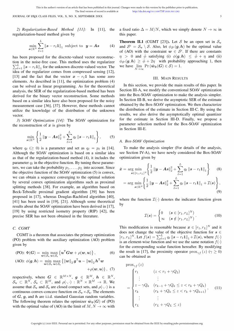
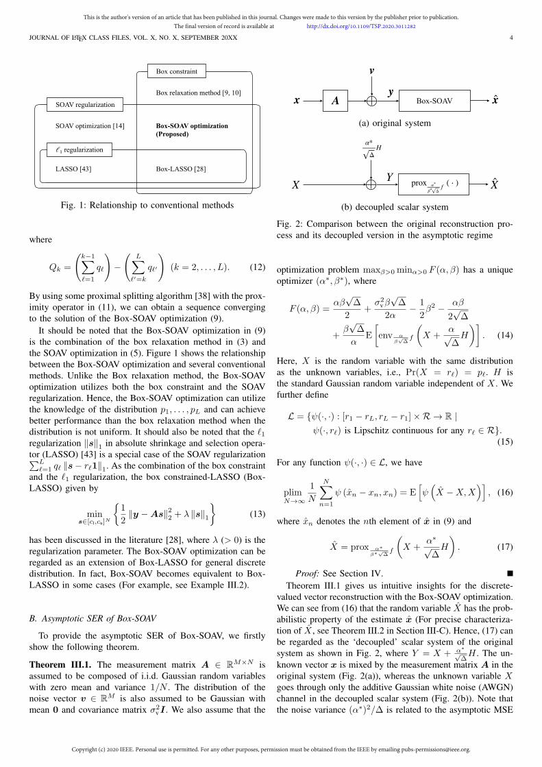

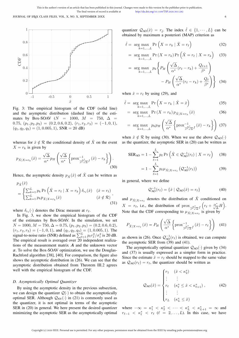


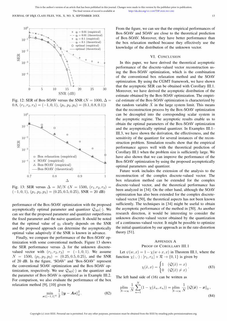

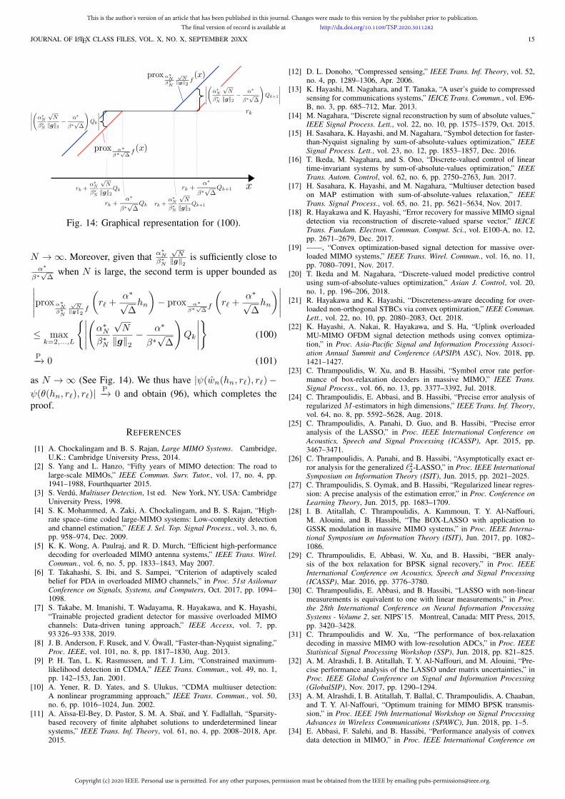


![· AXX+BXX 20xx- AXX 20xx x H ABC XX ABC BXX 20XX X F] ABC XX . 2019 20194 . 1 . h, POI ( ákJ* 30 2201 Elk 2.1 2.2 2.3 . Created Date: 9/9/2020 3:05:52 PM ...](https://static.documents.pub/doc/80x56/606e842847f51e6bfd5988c3/axxbxx-20xx-axx-20xx-x-h-abc-xx-abc-bxx-20xx-x-f-abc-xx-2019-20194-1-h.jpg)


