ATINER's Conference Paper Series COM2013-0658 · Teradata Inc USA Abstract The techniques of hash...

ATINER CONFERENCE PAPER SERIES No: COM2013-0658

1

Athens Institute for Education and Research

ATINER

ATINER's Conference Paper Series

COM2013-0658

Son Pham

Professor

California State University at Northridge

USA

Thu Pham

Senior Consultant

Teradata Inc

USA

Dynamic External Merger Sort for

Partial Group-by in Optimization


2


8 Valaoritou Street, Kolonaki, 10671 Athens, Greece

Tel: + 30 210 3634210 Fax: + 30 210 3634209

Email: [email protected] URL: www.atiner.gr

URL Conference Papers Series: www.atiner.gr/papers.htm

Printed in Athens, Greece by the Athens Institute for Education and Research.

All rights reserved. Reproduction is allowed for non-commercial purposes if the

source is fully acknowledged.

ISSN 2241-2891

31/10/2013


3

An Introduction to

ATINER's Conference Paper Series

ATINER started to publish this conference papers series in 2012. It includes only the

papers submitted for publication after they were presented at one of the conferences

organized by our Institute every year. The papers published in the series have not been

refereed and are published as they were submitted by the author. The series serves two

purposes. First, we want to disseminate the information as fast as possible. Second, by

doing so, the authors can receive comments useful to revise their papers before they

are considered for publication in one of ATINER's books, following our standard

procedures of a blind review.

Dr. Gregory T. Papanikos

President



4

This paper should be cited as follows:

Pham, S. and Pham, T. (2013) "Dynamic External Merger Sort for Partial

Group-by in Optimization" Athens: ATINER'S Conference Paper Series, No:

COM2013-0658.


5

Dynamic External Merger Sort for

Partial Group-by in Optimization

Son Pham

Professor

California State University at Northridge

USA

Thu Pham

Senior Consultant

Teradata Inc

USA

Abstract

The techniques of hash and sort/merge naturally compete for a join plan within

group-by queries because they both cluster records. Hash technique tends to

cluster faster than its rival short/merge (in special cases). Despite its

advantages, hash usually fails to yield a lower cost. In order to avoid such

problematic issues, several methods are proposed to improve these techniques

such as: apply the partial group-by operator in conjunction with the heap/merge

sort process to remove immediately duplicates; increase the input size by

coupling the runs in heap sort to reduce CPU time as well as the I/O time; and

utilize the feedback mechanism to extend each merge run to reduce further the

I/O processing.

Keywords:

Corresponding Author:


6

Introduction and Motivation

In SQL (Structure Query Language), group-by is an operator that clusters

collective data across multiple records by using a key with one or more

columns. It is viewed as removing duplicate records with identical keys and

clustering aggregate on another particular column. Group-by performs a

complete clustering once at the end of the join plans. Partial group-by operates

similarly but clusters partially throughout the join plans multiple times. In

either case, hash and sort/merge techniques can be used to achieve the same

results.

Sorting automatically arranges collective data into increasing or decreasing

sequence clusters. Sorting becomes difficult when RAM cannot hold all data

records. Therefore, it requires additional merge to complete its task. Initially,

RAM will be filled up to its capacity and then sorted. This sorted segment is

then stored as a run into a file. The process is repeated until all the collective

data is exhausted. In order to complete the task, all runs are merged to a sorted

single file. Nevertheless, this technique is complex and has high cost in both

CPU and I/O times.

Hashing also clusters records but does not sort. Hashing scans the

collective data and stores same-key records into a bucket. This is preferable for

lower cost because it scans data only once. However, it has some restrictions:

1) RAM must be large enough to hold all the buckets. Since each bucket only

holds one representative record and an updated aggregated value, RAM needs

to hold distinctive key records. 2) The number of distinct keys must be known

before hashing. If it is not known, the number must be counted and therefore

time consuming. Instead an estimation is done but at the cost of accuracy. This

presents a large error margin and may lead to an overflow of distinctive records

in the RAM. Consequently collisions will occur, i.e., two records with two

different keys end up in the same bucket. Completion time for clustering is

unpredictable and may even longer time than the rival merge/sort.

Hashing presents its own set of concerns. In an ideal case, there is an

abundance of duplicated and therefore less distinct keys. In a scarce duplicate

case, it may require large amounts of time or even fail to perform. In a case

where RAM capacity is in approximately close range of distinct keys, hashing

either performed reasonably well or poorly based on experimental data. If

hashing fails to perform, sort/merge is the last resort for optimizer to do

clustering. However, sort merge is complex and time consuming. As a result,

both techniques have disadvantages. In order to solve these concerns, new

techniques such as coupling technique and feedback mechanism are proposed

and used in conjunction with hashing/sort merge to enhance performance

Main Ideas for Solutions: Related Work

Many researchers have investigated the problem of group-by moving

around[7,9]. However, the implementation doe not encourage them to go


7

further due to the high cost of group-by[2,3]. In other words, optimizer would

not select group-by before the joins. Consequently the group-by was not fully

developed[8]. In parallel, the materialized views are growing with a lot of

promising in the queries using aggregation using the intermediate existing

views because the cost is reduced[5]. However, an extra cost should be

compensated: the cost for searching the appropriate views[4,6]. Therefore the

materialized view techniques make the group-by less attractive and hence

dampened the hope of group-by. On another aspect, the process of elimination

is still primitive to help group-by to achieve a significant reduction.

Group-by as an Elimination Process

Group-by operator can be viewed as an elimination process when the table

is sorted on the group-by fields[1]. During the row elimination, the aggregation

is updated. We name this process Group-by elimination. The elimination can

be done concurrently during the sorting. We attempt to reduce the CPU time

and I/O time. The sooner the rows are eliminated, the higher chance for the

lower I/O cost in the subsequent operation.

A. Heap sort:

In the external merge sort, the first pass, PASS 0 is the heap sort. In this

pass, the buffer is filled will rows. Then rows are sorted before it is dumped to

disk to make a run. Heap sort can be improved to remove the duplicates and

update the aggregations. Here is the comparison of the classical way and the

new improved one:

- In the classical way, the heap sort finishes its job first, and then

we build a routine scan the array to remove duplicates. The scan

running time is of order(n) where n is the size of the array.

- The more efficient way is to eliminate the duplicates during the

“delete step” of the root by moving it to the bottom right node of

the tree. We note that heap sort has two main steps: Step 1: to

build the heap structure and Step 2: to delete the root by

exchanging it with the bottom-right node of the tree, fix the heap

with a shorter than 1 element, and repeat the deletion. At this step

2, we might want to modify as follows: in the case of duplicate,

instead of exchanging, we only move the bottom-right node to the

root. We are able to keep tract the duplicate count at this moment

or to update the aggregation

In this section we will demonstrate the following features:

a. To incorporate the elimination process during the process of heap

sort. This will save the scanning CPU time for removing


8

duplicates. The saving is about O(n), where n is the cardinality of

the relation.

b. In addition, we will show a technique to implement the heap sort

in view of child-parent tree and the array tree so that the result (a

run) will be in an increasing order without duplicates. It will

occupy the original array from index 0 until to the new length of

the distinct elements.

c. The run can be stored block by block into the disk, instead of row

by row. Hence the average cost of I/O time per write will be

reduced.

d. Moreover, the run can be expanded. This will reduce the number

of runs under the modified heap sort process.

The section is divided into two parts: OVERVIEW ARRAY AS A

BINARY TREE and IMPLEMENTATION TO REMOVE DUPLICATES

A. OVERVIEW ARRAY AS A BINARY TREE

1a. Given a sequence of numbers, we can store it into an array as follows:

The sequence of numbers is filled in starting at the index 0.

Example: the sequence 92, 47, 21, 20, 12, 45 63, 61, 17, 55 37, 25, 64,

83, and 73 is stored in the array as follows:

1b. View the array as a tree as follows: (See Figure 1 for example of heap)

a. Root is at the last index (index = 5) of the array

b. Two children of the root are at the indices 4 and 3

c. The children of next level are at the indices 2, 1, and 0.

B. IMPLEMENTATION TO REMOVE DUPLICATES

a. Install heap sort: We follow the classical techniques to build the heap tree

with the above transformation between the array indexes and the

children/parent tree. Here is the pseudo code:

// Build the array with the heap property: parent is greater than or equal to

children

for( int i = Length / 2; i > 0; i-- ) percDown2( a, i, Length );

// PercDown2 fixes the heap at parent node I of the array a, limited within

the Length

// A loop: Delete the root, move the bottom-right node to the root, fix heap

at the root.

for( int i = Length; i > 0; i-- )

{ //i = size of array

percDown2( a, 1, i);

( index) 0 1 2 3 4 5

74 45 26 17 44 69


9

}// end For

Implement duplicate removal, and keep track of the counts of duplicates: We can extend the array to the array of records with fields: key and count,

where count is initialized to be 1. During the loop of the root deletion, we can

modify to remove the array is growing from index 0 to LastIndex-1 if we have

no duplicate in key. Otherwise, the resulting array remains the same length

except the count is updated. In the following, we will use Java-like Pseudo-

code to express the algorithm.

// Set LastIndex to be 0

LastIndex =0;

// first time to swap: delete root and move the bottom-right node to

root.

Record temp = a[rootA]; // hold the root after swap

a[rootA] = a[0];// delete root: the last index in the array

a[0] = temp;

Figure 1: Tree and index for heap structure.

Formula of transformation:

iP + iA = n, where iP is an index in the parent/children tree, iA is its

corresponding node in the array tree and n is the length of the array

if i is a parent, 2*i and 2*i+1 are two children.

Index

5 6

9

Index

4

Index

3

Index

2

Index

1

Index

0

4

5

2

6

7

4

1

7

4

4

Tree of Array Indexes

1

6

9

2 3

4 5 6

4

5

2

6

7

4

1

7

4

4

Tree of Parent/Children Indexes


10

LastIndex++;

// second and after with elimination of duplicates.

for( int i = rootA; i > 0; i-- )

{

percDown2( a, 1, i); // 1 and i are two ends of children-

parent tree

// add codes to remove duplicates.

if (a[rootA].key== temp.key)

{ // count up for duplication

a[LastIndex -1].count += a[rootA].count;

a[rootA] = a[Length-i]; // move last element up

}

else if (Length-i==LastIndex)

{ temp = a[rootA];

swapReferences( a, rootA, Length-i );

LastIndex++;

}

else

{ a[LastIndex] = a[rootA];

a[rootA] = a[Length-i];

temp = a[LastIndex];

LastIndex++;

}

}// end For

return LastIndex;

NOTES:

1. In Appendix A is a Java program for heap sort with removal duplicates and

keep track of the count of the duplicates.

2. The technique demonstrates the removal duplicates and concurrently

keeping track of the count. However, it is used count as an example

without loss of generality. It can do similarly to update aggregations as

long as the aggregations are decomposable such as Min, Max, SUM, and

the like. Decomposable means the aggregation on a subset of rows can be

carried to the super set.

Discussion

1. If RAM can hold the distinctive records, the heap can eliminated all

duplicated with a single run. This is the case of hashing.

2. In other cases, multiple runs will be generated and the merging the runs

will be required to remove further the cross-over duplicates among the

runs. We will discuss this topic in the merging section. Nevertheless, the

number of duplicates in the collected records can be contributed


11

significantly in the I/O reductions. The large number of duplicates, the

more reduction in I/O.

3. The removing duplicates instantly in sort/merge processes will integrate the

two techniques hashing and sorting not to have a two extreme costs but a

gradually costs base on the number of duplicates.

B. The Theory on the Removal

In this section, we will investigate the number of removal duplicates using

probability. A key is a set of one or more attributes, which is subject to be

removed its duplicates. Without loss of generality we assume a key of one

attribute, instead of multiple attributes. We assume that the key values are

randomly distributed within the table. We further assume that the keys are

duplicated evenly. We introduce the following notations:

- Let n be the number of distinct values of the key. It can be calculated

as the ratio of the table cardinality and the number of duplicates per

value.

- Let B be the number of rows can be hold by the system buffer. It can be

calculated by the formula:

B = (size of buffer in bytes)/ (size of the row in bytes).

The size of B can be smaller or larger than the number of distinct keys n.

In the case of B < n, the duplicates in B is possible due to the repetition in the

table. However, the number of duplicates will be much less than the one in the

case of B>= n. In this section, we will estimate the number of the removals in

the buffer.

Definition 1: Given a table. If it has two rows of the same key and no

other rows have that key, we say it has a pair of identical key – call pair for

short. Similarly we call triple, quadruple, quintuple for the cases of three

identical keys, four identical keys, and five identical keys respectively. In

general, if it has k rows of the same key, we say it has a k-identical. Hence

pair, triple, quadruple, and quintuple are 2-identical, 3-identical, 4-identical and

5-identical respectively. In this definition, triple is not two pairs.

This definition can be generalized for a subset of a table instead of the

whole table.

Lemma 1: The chance for a buffer B to have a pair is

where is B!/(2! * (B-2)!). B

2

B

2 n * (n-1)B-2

n B


12

Proof: There are n B combinations of B rows for n possible rows of n

distinct keys. We want to find the number of pairs in these combinations. For

convenient, we use the keys 0,…(n-1) for n possible keys and consider B as an

array of B rows. Since each pair will occupy two rows in the buffer of B rows,

there will be B!/(2! * (B-2)!) choices. For each B-choice, we can have the key

0,...(n-1) for the pairs.

Consider one choice with key = 0, there are remaining B-2 spaces in the

array. These spaces cannot hold key 0 because the key 0 already appeared.

Otherwise we don’t have pair in this choice. Therefore there are n-1 distinct

keys for (B-2) spaces. Certainly we have (n-1) B-2

combinations of n-1 distinct

keys for B-2 spaces; there are possible some more pairs within them; hence the

new pair make B-choice having the double pairs. Let k be the number of pairs

in these combinations. Hence (n-1) B-2

- k is the number of combinations

without pairs. Therefore we have:

Number of single pairs of key 0: B!/(2! * (B-2)!) * ( (n-1) B-2

- k).

Number of double pairs of non-zero keys: B!/(2! * (B-2)!) * k.

We can repeat the same logic for other keys 1,..n-1. Hence we have in

total the following

single pairs: n * B!/(2! * (B-2)!) * ((n-1) B-2

- k)

double pairs: (n/2) * B!/(2! * (B-2)!) * (k).

In the double-pair case, the number of double pairs will be cut down a half

because for each double-pair row, there will be another copy in later case. We

can demonstrate as follows: the B-buffer (-, -, -, i, -, -, -,i, -, -, -, j, -, -, -,j…)

can be generated with the pair (i, i) from one of the B!/(2! * (B-2)!) choices

and the pair (j, j) from one of the pairs in B-2 spaces. This combination can

also be generated with the pair (j, j) from one of the B!/(2! * (B-2)!) choices

and the pair (i, i) from one of the pairs in B-2 spaces. Hence if we count one for

each single pair and count 2 for each double pair, we have the following total

number of pairs: n * B!/(2! * (B-2)!) * (n-1) B-2

. Therefore the proof is

completed.

Lemma 2: The chance for a buffer B to have a j-identical is

where is B!/(j! * (B-j)!).

Proof: The proof is similar to the one of Lemma 1.

Proposition 1: The number of removal duplicates in the buffer is

B

j

B

j n * (n-1)B - j

n B


13

where is B!/(j! * (B-j)!).

The number of distinct keys in the buffer is

Proof: For each j-identical, we can remove j-1 out so that all keys are distinct.

Hence the numbers of rows can be removed out of B-buffer is the total

removals of all j-identical, where j = 2..B.

For the second formula, the logic can be simple. The keys from the table have

n distinct values. For one fixed key, the chance for not-selecting it is (n-1)/n.

For the buffer of size B, the chance for not selecting the key is [(n-1)/n]B

.

Hence the chance for selecting the key is 1- [(n-1)/n]B

. For all n keys, the

chance for them to be selected in the buffer is n*[1-(n-1)/n]B

.

Computer simulation for the removal of duplicates: (See Table 1)

In this section we will write a program to generate n different keys of

integers and duplicate them multiple times. The keys are then permuted

randomly. The B keys are extracted sequencially from the generated source.

Then we inspect their duplicates and is calculated by sum of all removals over

the number of extractions. Table1 includes some results from the formula given

by Proposition 1 and by the simulation on the varieties of buffer size B and

different number of distinct keys.

Behavior of Removals with respect to the Base:

Table1: Some comparisons of row reductions provided by the formula in Proposition 1 and by computer simulation.

(a) (b) (c) (d)

3 4 0.6875 0.6970

4 5 1.0480 1.058

5 7 1.238651 1.225715

6 4 2.71191 2.7025

7 5 3.048576 3.04325

9 4 5.300339 5.299

(a): the buffer size in rows

(b): the distinct key values

of the table.

(c): the row reduction in

buffer due to the removal of

duplicates provided by

Proposition 1.

(d): the average of row

reduction provided by

computer simulation.

B

j=2

B

j n * (n-1)B – j * (j-1)

n B

B

j

n * (1 – [(n-1)/n]B )


14

We still assume that each key value is duplicated uniformly across the

table. The base is defined as the ratio of the table cardinality over the number

of duplicates per key. This is also the number of the distinct values in the

table. In Chart 1, with the fixed buffer size = 15, we plot the row reduction of

buffer when the base is changed. The graph indicates a hyperbola shape: as the

base is increasing, the row reduction is decreasing. On the other hand, in Chart

2, with the fixed base = 14, we plot the row reduction of the buffer when the

buffer size is changed. In this case we have a parabola shape.

Programming experiment 2: We configure the buffer of size B = 15 and

generate a relation of 600 records from 60 distinct keys. These keys are

permuted randomly. Each load from the relation to buffer will be removed the

duplicates to the distinct keys. With eight independent executions, we have the

following sequence of the new lengths of runs: 12/15/14/13/12/14/14/15. Their

average is 13.625.

Coupling Technique

In this section we will introduce a technique named coupling to extend the

sizes of runs during the removal duplicates. The records from the collected data


15

will be read in sector to fill the read buffer. It is transformed to RAM for heap

sorting with concurrently removal duplicates. After sorting, the sorted segment

will be moved to the output buffer except for the last record with the largest

key. The output buffer is not filled up yet because of the duplicate removal

and it will not be written to file until it is filled. In the meantime the read buffer

is filled up with the next read sector for the next run. RAM is sorted with

duplicate removal. The last key of the previous run is used to locate within this

sorted RAM to find the record with first equal or larger key. At this point, the

output buffer will be more filled. The output buffer is written to file when it is

filled.

Note: In practice, the file system might be different. However, the concept is

the same-- remove duplicates as soon as possible, extend the input length, and

delay the output until it is filled.

Figure 2 depicts the steps of a coupling technique: 1) Read the collected

data to RAM; 2) heap sort on RAM with duplicate removal; 3) Write RAM to

output buffer and keep the last key; 4) Read the next sector of the collected

data to RAM; 5) heap sort on RAM with duplicate removal 6) Use the last key

of step 3 to locate the record in RAM; 7) fill up the output buffer.

Figure 2. Comparison the Common technique to the Coupling


16

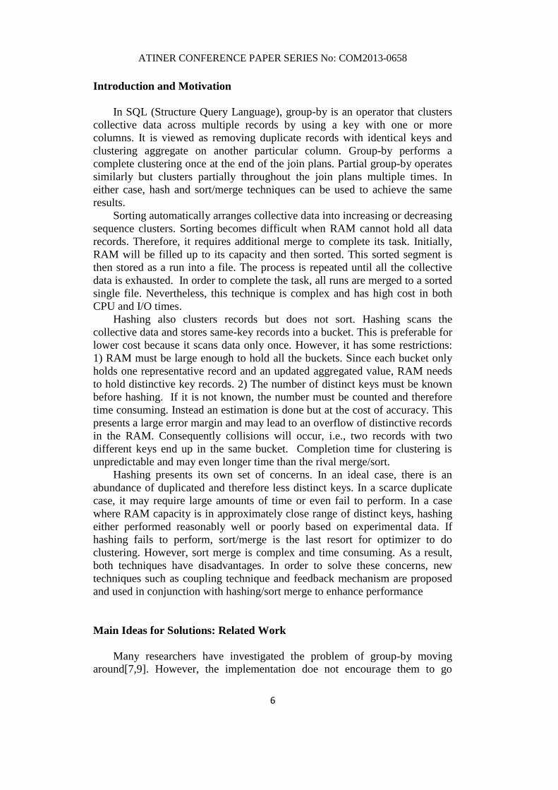
Figure 3. Provides the chart of reduction in runs with coupling technique. We

observe that the more distinct keys, the less reductions in runs

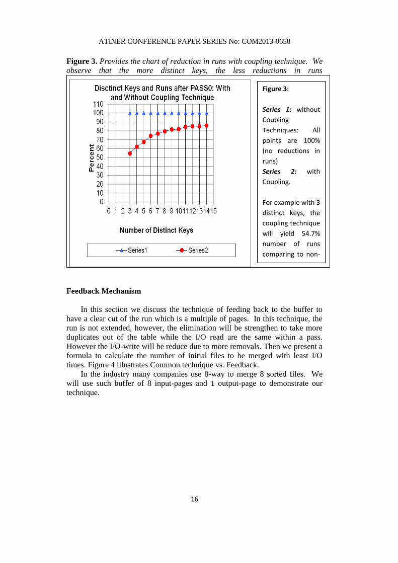
Feedback Mechanism

In this section we discuss the technique of feeding back to the buffer to

have a clear cut of the run which is a multiple of pages. In this technique, the

run is not extended, however, the elimination will be strengthen to take more

duplicates out of the table while the I/O read are the same within a pass.

However the I/O-write will be reduce due to more removals. Then we present a

formula to calculate the number of initial files to be merged with least I/O

times. Figure 4 illustrates Common technique vs. Feedback.

In the industry many companies use 8-way to merge 8 sorted files. We

will use such buffer of 8 input-pages and 1 output-page to demonstrate our

technique.

Figure 3:

Series 1: without

Coupling

Techniques: All

points are 100%

(no reductions in

runs)

Series 2: with

Coupling.

For example with 3

distinct keys, the

coupling technique

will yield 54.7%

number of runs

comparing to non-

coupling

technique.


17

Figure 4. Common Technique vs. Feedback

Conclusion

The common technique will yield a binary decision either hash or sort/

merge. The decision is based on the capacity of RAM; whether it can hold all

the distinct keys or not. If the all the distinct keys can be fitted into RAM,

there will be only one run and the hashing technique is applied. The graph in

Figure 3 depicts a gradually decrease in reductions of the runs when there are

more distinct keys. Hence the costs for group-by operator with this coupling

technique will yield a varying range of cost, not the binary costs from the

common technique.

From a different perspective, duplicates in heap are removed within a run

(intra duplicates) while merge eliminates the duplicates from cross runs (inter-

duplicates). Therefore, more studies are needed to understand heap and merge

behavior. Since the heap is performed first, all inter-duplicates are removed

within each individual run. The remaining inter-duplicates are only in cross

runs. Therefore further studies on the inter-duplicates are necessary. Some

preliminary experiments are conducted on several TPC-benchmarks

(Transaction Processing Performance Council) group-by queries. One

experiment will remove inter-duplicates right after the heap, and the other will

delay removal until the end of join plans. The latter case is faster about 20%

to 40%. More study should address questions such as: How many inter-

duplicates are there in the merge? When to remove the duplicates right after

the heap or postpone until the end of the join plan?” Such questions are

currently under research to truly understand the removal of duplicates.


18

References

Chaudhuri, S and Shim, K.1994). Including Group-By in Query Optimization, (In

VLBD, pp. 354-366.

Gray,J., Bosworth, A., Layman, A, and Pirahesh, H. (1996) Data cube: A relational

aggregation operator generalizing group-by, cross-tab, and sub-totals. In

Proceeding 12th International Conference on Data Engineering, New Orleans,

Louisiana USA, February.

Grumbach, S. et al.(1999), Querying Aggregate Data, PODS '99, pp. 174-185.

Gupta, A. (1995) "Generalized Projections: A Powerful Approach to Aggregation,"

VLBD, pp. 1-26 (1995).

Larson, P.A. and Yang, H.Z.(1985) Computing queries from derived relations. In

VLDB, pp. 259-269.

Rafanelli, M., Bezenchek, A. and Tininini, L.(1996) The aggregate data problem: a

system for their definition and management. ACM Sigmod Record, 25(4): 8-13,

December.

Pham, S. and Pham, T. (2005) Group-by Early in Optimization. In: Computer Science

and Information System Edited by Dr. Panagiotis Petratos & Dr. Demitrios

Michalopoulos, 411-430.

Pham, S. and Pham, T. (2008) Sorting of records with duplicate removal in a

database system US Patent: 7370068.

Yang, H. Z. and P. A. Larson, P. A. (1987) Query transformation for PSJ-queries. In

VLBD, pp. 245-254, 1987.


19

Date post:	27-Aug-2018
Category:	Documents
Upload:	ngonhan
View:	212 times
Download:	0 times

ATINER's Conference Paper Series COM2013-0658 · Teradata Inc USA Abstract The techniques of hash...

Documents