ATIS Graph Theory - Indiana University Bloomington · ATIS Graph Theory ATIS Graph Theory is...

© Copyright 1996 to 2008 by Kenneth R. Thompson, Systems Predictive Technologies, 2096 Elmore Avenue, Columbus, Ohio 43224-5019;

Site: www.Raven58Technologies.com. All rights reserved. Intellectual materials contained herein may not be copied or summarized without written permission from the author.

System-Predictive Technologies Report # 11 October 7, 2007

The report number corresponds to the Proffitt Grant report of the same number

Updated March 2008

ATIS Graph Theory

Prepared by: Kenneth R. Thompson Head Researcher

System Predictive Technologies 2096 Elmore Avenue

Columbus, Ohio 43224-5019

Prepared as an independent report for Theodore W. Frick, SimEd & MAPSAT Development Head Researcher

Associate Professor and Web Director School of Education Indiana University

Bloomington, Indiana

ATIS Graph Theory, Report 11 – 1



ATIS Graph Theory

ATIS Graph Theory is developed directly from the definition of system with GO, the object-

set, and GA

, the relation-set, as the basis for the theory. This development is required in order to

obtain the analyses that determine the Structural Properties of the target system and the

corresponding axioms. These axioms will then provide the means to predict behavioral outcomes

of the system.

This development will start with a diagram of a system and its main partitions and source of its affect-relations.

Graph theory is founded on the notion of vertex, v, as the only primitive term and edge, e, defined in terms of the system vertices. For ATIS, v∈GO and e∈G

A.

The construction of GO and GA

are defined on the following two pages.

This report is a revision of the Proffitt Grant report of the same number, and has been refined to reflect a more in-depth analysis of ATIS Graph Theory. This report, in particular, will provide various definitions whose measures are determined by the Shortest Distance Measure defined by the Floyd-Warshall Algorithm. This algorithm provides the shortest distance; i.e., path lengths, between every two system components. Having established these distances, then path lengths between any two components can be determined as a sum of shortest paths as an application of the Transitive Property for Ordered Pairs. That is, if (x,y) and (y,z) define direct affect relations from x to y and y to z, respectively, then there is an indirect affect relation, (x,z), from x to z that has a path link that is the sum of the two direct affect relations.

Determining all direct and transitive ordered pairs will define all system shortest-path affect-relations.

As of March 2008, this report is being updated to provide a more thorough discussion of ATIS Graph Theory and other topics not previously discussed. Some of the current updates are derived from the text: Network Analysis, Methodological Foundations, by Ulrik Brandes and Thomas Erlebach (Eds.), Springer-Verlag, Berlin and Heidelberg, Germany, 2005.




The System Relation-Set, GA, is defined as follows:

Affect Relation-Set, GA

, Construction Decision Procedure

The logical construction of the affect relation-set, GA, will be determined as

follows:

1) Every Information Base (ĪB) defines affect relations, An∈A, by the unary- and binary-component-derived sets from the ĪB. That is, the components of An are of the form: {{xi},{xi,yi}} ∈ Ai∈An that indicates that an “affect relation” has been determined to exist from “xi” to “yi.”

2) Affect Relation-Set Predicate Schemas, P(xn,yn) = P(An), are defined as required to define the family of affect-relations, An∈A, as extensions of the predicate schemas. ‘P(An)’ designates the predicate that defines the components of An.

3) The Affect-Relation Transition Function, φn, is defined by:

φn: X×Y → An | X,Y ⊂ ĪB .∧. φn(X×Y) =

{{xn},{xn,yn}}| P(An) ∧ xn∈X ∧ yn∈Y}.

4) The family of affect relations, A = GA, is defined recursively by applications of

the function defined in 3) for all elements in ĪB to each P(An) defined in 2).

5) New components are evaluated for each P(An) defined in 2) and included in the appropriate extension when the value is true.

6) No other objects will be considered as elements of An∈A = GA except as they are

generated in accordance with rules 1) through 5).




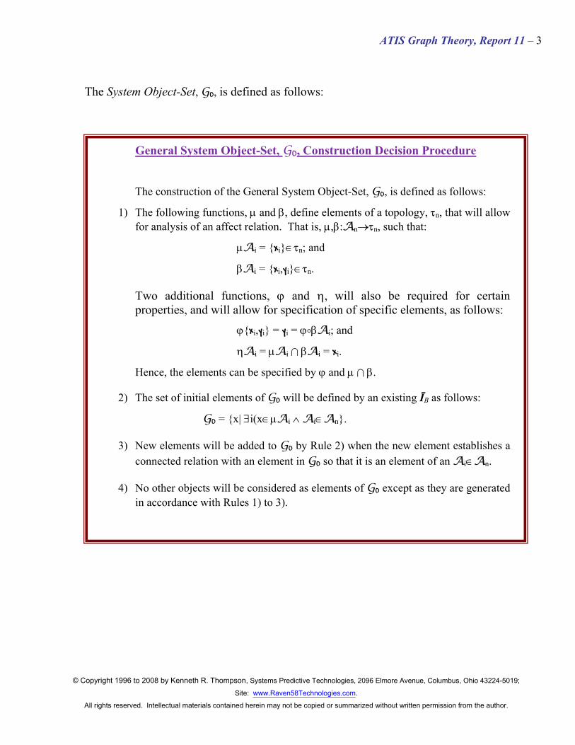
The System Object-Set, GO, is defined as follows:

General System Object-Set, GO, Construction Decision Procedure

The construction of the General System Object-Set, GO, is defined as follows:

1) The following functions, µ and β, define elements of a topology, τn, that will allow for analysis of an affect relation. That is, µ,β:An→τn, such that:

µAi = {xi}∈τn; and

βAi = {xi,yi}∈τn.

Two additional functions, ϕ and η, will also be required for certain properties, and will allow for specification of specific elements, as follows: ϕ{xi,yi} = yi = ϕ)βAi; and

ηAi = µAi 3 βAi = xi.

Hence, the elements can be specified by ϕ and µ 3 β.

2) The set of initial elements of GO will be defined by an existing ĪB as follows:

GO = {x| ∃i(x∈µAi ∧ Ai∈An}.

3) New elements will be added to GO by Rule 2) when the new element establishes a connected relation with an element in GO so that it is an element of an Ai∈An.

4) No other objects will be considered as elements of GO except as they are generated in accordance with Rules 1) to 3).




Global Graph of System Properties

A system is quite complex and exhibits many different interrelations of its components. A General System Graph is shown below in Diagram S-1. ‘G’ =df General System

Diagram S-1 Universe of Discourse (U) G = df (P, A, T, Q, σ)1,2

1 G is the General System, P is the Object Partitioning Set, A is the Family of Affect Relations Set, T is the Linearly Ordered Time Set, Q is the Qualifier Set, and σ is the System State Transition Function. 2 TP, IP, FP, OP, SP, L, L ’, SBX, S’BY ∈ P (‘BX’ & ‘BY’ are the “background components”); A1, A2, …, An ∈A; t1, t2, …, tk ∈T; fI, fO, fT, fB, fS ∈T.




In Diagram S-1, the system components are the endvertices of the “arrows”. In this case, the components are partitions (or partition-subsets) of the system; i.e., input, output, storeput, etc.

Diagram S-1 also indicates the various Basic, Structural and Dynamic Properties of the system.

An analysis of a system can become very complex. This complexity increases even more when a full General System Multi-Level Graph as shown on the following page in Diagram S-2 is analyzed. The graph shown is a 3-Tier Graph that includes an analysis of a supersystem and subsystems.

General System 3-Tier Graph

System analyses are most often, if not always, restricted to well-defined systems that ignore the environment of the system as well as subsystems. This frequently is done simply to have more control over the research being conducted, and, in fact, may explain the reliance on statistical-based analyses; that is, they are essential since the total relevant system is not being analyzed at the component-level. However, it is also for this reason that most, if not all, social science projects, in particular, are flawed and provide somewhat or substantial invalid results. Diagram S-2 provides a glimpse as to why this is.




Diagram S-2

Target System; e.g., a high school

Target System’s Supersystem; e.g., the environment of the high school to include other high schools, middle schools that feed the high school; the controlling school board, etc.; the fire, police, and medical infrastructure; home, religious and social support groups, etc.

Target System’s Subsystems; e.g., classrooms, principal’s office, counseling department, athletic organizations, in-school medical and security organizations, etc.




As can be seen, a comprehensive system analysis is very daunting since the super-system

and all relevant subsystems must be analyzed as separate systems and then be integrated with the target system to determine their effect and the resulting predictive outcomes.

General System Multi-Level Analysis

As can be seen from Diagram S-2, a full analysis of a system should include at least an analysis of the main subsystems and their relation to the entire system even if the supersystem is not analyzed, which could result in a very large system. However, in most cases, even subsystems are not analyzed in the research conducted by social scientists. However, the analysis needs to be even more comprehensive. Once a targeted system is defined for analysis, the relevant supersystems and subsystems must also be identified. Once they are identified, then an analysis of each of these systems needs to be completed and then integrated with the analysis of the targeted system to obtain the desired analysis.




ATIS Overview

Graph Theory provides the basis for many disciplines in which there is a connectedness of elements or components that seem to be related in a system-type arrangement. Graph Theory provided an integral part of SIGGS (Set Theory, Information Theory, Graph Theory, and General Systems Theory) that was devised by Elizabeth Steiner (Maccia) and George Maccia in the 1960’s. More recently, it has provided a basis for studies of Networks and Social Networks, in particular. Much of Network Analysis, however, is designed around Internet-type systems and frequently relies on communications between components derived from Information Theory. In all instances, the development of network-type analyses relies on statistical-based analyses.

ATIS has been designed as an axiomatic theory that is not dependent on either Information Theory or statistical-based analyses. For that reason, this report presents ATIS Graph Theory, and will utilize only those graph-theoretic concepts that are applicable to this theory, which may include certain axioms related to Graph Theory.

ATIS Graph Theory

Vertex (Component). We start with one primitive term: vertex (component), v.

Vertices (components) are elements of a set, GO; that is, v∈GO. In Diagram 1, all of the lettered “boxes” are vertices (components). [Vertices will be referred to as components for the rest of this report.]

Edge (Affect-Relation). An edge (affect-relation), e, is mapped onto an element of the product GO%GO where the elements from each GO are the endvertices (end-components) of the edge (affect-relation). In Diagram 1 shown below, the edges (affect-relations) are the non-directed or directed arrows between the components. Note that (k,l) is a non-directed edge. [Edges will be referred to as affect-relations for the rest of this report.]

Therefore, GA = GO%GO.




Non-Directed Affect-Relation. A non-directed affect-relation, e, is an affect-relation that does not have an initiating or terminating end-component; that is, it is not directed. For non-directed affect-relations, GO is not partitioned. In Diagram 0, GO consists of all end-components. Diagram 0 represents a graph of the components and affect-relations. (Graph will be formally defined below.) The non-directed affect-relations are those that do not have the arrowheads; i.e., {k, l} = {l, k}. Non-directed affect-relations are designated by a binary set containing the end-components of the affect-relation.

Mixed Graphs. A mixed graph is a graph that has both non-directed and directed affect-relations. Diagram 0 presents a mixed graph. Unlike for most systems or networks, it is likely that many of the systems that are analyzed under ATIS will be depicted by mixed graphs; i.e., many systems will have both known directed affect-relations and those that are unknown except for the components involved which will have to be depicted by non-directed affect-relations. For example, it may be known that two students work together to complete their homework; however, it may be unknown which one, if either, is helping the other and would be identified by the affect-relation controls activities of. In such a system, the relation can be identified as a non-directed affect-relation. In such systems, there will be two functions defining the mappings of the components:

(1) For non-directed affect-relations, ƒ:A → GO%GO.

(2) For directed affect-relations, ƒ:A → IGO%TGO.

Incidence Relation. An incidence relation is the relation defined by relations (1) and (2) above; i.e., an incidence relation defines the system relation-set to the system object-set.

As a result of this definition, we will say that affect-relations are incident to their respective end-components.

Directed Affect-Relation. A directed affect-relation, e, is an affect-relation that has both an initiating and terminating end-component; that is, GO is divided into initiating-components, IGO, and terminating-components, TGO, so that (vi,vj)∈ IGO%TGO where IGO 4 TGO = GO but the sets are not necessarily disjoint. In Diagram 0, IGO consists of the end-components that do not have the arrowheads, and TGO consists of the end-components that do have the arrowheads.

Since the notion of a simple graph depends only on the definition of directed affect-relation, it will now be defined so that it can be used in some of the later definitions. It will also be defined later as part of the definitions concerning various types of graphs.




Diagram 0

Simple Affect-Relation. A simple affect-relation is an affect-relation that maps onto only one component.

In Diagram 0, all affect-relations are simple affect-relations.

Simple Graph, or Simple Affect-Relation Graph. A simple graph, or simple affect-relation graph, is a graph that contains only simple affect-relations with no loops, cycles, or parallels (hyper-affect-relations) which will be defined later.

Affect-Relation Basis (Undirected Affect-Relations). An affect-relation basis (undirected affect-relations) are the affect-relations without the directed links; i.e., a mapping of undirected affect-relations.

Affect-Relation Basis Graph. An affect-relation basis graph is a graph that contains only undirected affect-relations.

This graph may be required in order to determine the connectedness of any two components.

a

i

h

g

jd

c

fe

b

k

l

m




Component Degree. The component degree, d(v), is the number of affect-relations incident to v; that is, that emanate from v or are initiated at v.

Component degree is dependent on the affect relations being analyzed and whether or not

the analysis is concerned with only one affect relation or a hyper-affect relation; that is, when there

is more than one type of affect-relation, as well as whether both initiating and terminating relations

are considered or taken individually.

In Diagram 1, the component degree of j is 3; i.e., d(j) = 3, since there are three affect

relations initiating or terminating with respect to j, and assuming that all relations incident to j are

being analyzed

Diagram 1a provides a greater challenge since there are three different affect relations in the

graph. What is the value of d(d)? There are at least four different values: dH(d) = 6, d1(d) = 3,

d2(d) = 2, and d3(d) = 1, for the hyper-affect-relation, and affect-relation-1, -2, and -3, respectively.

But, as will be seen below, there are actually some more alternatives, so you must be precise when

defining the affect relations of concern.

Diagram 1

In Diagram 1, both (a, e, f, i, j, i, f, g, h) and (a, b, d, c, b, a, e, f, i, j, m, j, i, f, e) are walks

a

i

h

g

jd

c

fe

b

k

l

m




Diagram 1a

Initiating-Component Degree. The initiating component degree, dI(v), is the number of

affect-relations incident to v that are initiating affect-relations.

Terminating-Component Degree. The terminating component degree, dT(v), is the

number of affect-relations incident to v that are terminating affect-relations.

In Diagram 1a, the component degree of d is:

For Initiating and Terminating Hyper-Affect Relations: dHI(d) = 3, dHT(d) = 3,

For Two Affect Relations: dH(1-2)I(d) = 3, dH(1-2)T(d) = 2, dH(1-3)I(d) = 1, dH(1-3)T(d) = 2, dH(2-3)I(d) = 1,

dH(2-3)T(d) = 2,

For Initiating-Affect Relations: d1I(d) = 2, d2I(d) = 1, d3I(d) = 0,

For Terminating-Affect Relations: d1T(d) = 1, d2T(d) = 1, d3T(d) = 1.

a

g

c

fe

b

h

d

Affect relation #1 Affect relation #2 Affect relation #3




Disjoint Component. A disjoint component, v, is a component such that: d(v) = 0; i.e., it is not connected to any other component.

If a component is actually not connected to any other system component by any affect-relation, then, by definition, it cannot be recognized. However, with most empirical systems, every component will be connected to other components by at least one type of affect-relation. Under such a system, a component may be a disjoint component with respect to one or more affect-relations while being connected by other affect-relations that establish its identity within the system.

Bridge. A bridge, e, is an affect-relation such that if it is removed will make the end-components disjoint.

For certain analyses, one may wish to focus on a specific component and its affect-relations. To do so, the set of affect-relations incident to that component must be known. Such a set is identified by ‘Γ’. In Diagram 1a, Γ(d) = {(d,b)1, (d,d)1, (d,d)2, (c,d)3}; where the subscripts indicate the affect-relation.

Component Affect-Relation Set. The component affect-relation set, Γ(v), is the set of affect-relations incident to v.

For ATIS, Γ(v) ∈ An ⊂ A.

The component affect-relation set with initiating affect-relations at v is ΓI(v); and the component affect-relation set with terminating affect-relations at v is ΓT(v).

Further, another important set is the component neighborhood set. This is the set of all components that are directly-connected to a component. Such a set is identified by ‘N’.

Component Neighborhood Set. The component neighborhood set, N(v), is the set of components that are directly-connected to v.

For ATIS, N(v) ⊂ GO.

The neighborhood affect-relation set with initiating affect-relations at v is NI(v); and the component affect-relation set with terminating affect-relations at v is NT(v).




Walk. A walk is an alternating sequence of components and affect-relations, beginning and ending with a component, regardless of path direction, if any. Essentially, to determine a walk, a graph is viewed as a non-directed graph. And, this will facilitate one of the most basic concepts encountered in General Systems Theory from which ATIS has been retroduced: Components are connected if a walk exists from one component to the other, otherwise they are disconnected. A walk also determines whether or not one component affects another component is some way. If a walk exists between the components, then there is an affect relation of some kind between them, and the behavior of the system is determined, in part, by this relation.

Directed-Walk. A directed-walk is an alternating sequence of components and affect-relations, beginning and ending with a component, in which path direction is critical; that is the alternating sequence of components must start with a component that is an initiating end-component of the affect-relation and the subsequent component must be a terminating end-component that is also the initiating end-component of the next affect-relation, and the sequence continues to alternate with such affect-relations.

NOTE: If d(v) ≥ 2, then a directed-walk may continue in any direction if the terminating

end-component has more than one subsequent initiating end-components.

NOTE: Also of concern, as with the definition of degree, is whether or not the directed-walk must be with respect to the same affect-relation or if different affect-relations may be used to continue the directed-walk. In the latter case, Hyper-Affect-Relations are considered, whereas in the first case all affect-relations must be the same. This same consideration must be accounted for even in a non-directed graph, since the paths will be different if different affect-relations are allowed. How components are connected is a matter of choice that may depend on the analysis being conducted. Further, if, with respect to one affect relation, two components are not connected but are connected with another affect relation, then these components are connected with respect to the hyper-affect relation even if they are not connected with respect to one of the affect relations. Again, these components do in some manner modify the system behavior by their hyper-affect relation connectedness.

Trail. A trail is an alternating sequence of components and affect-relations, beginning and ending with a component, regardless of path direction, if any, and all affect-relations are distinct; i.e., the walk does not retrace itself, no affect-relation occurs more than once.




Closed Walk. A closed walk is one in which the initial and final components are the same.

In Diagram 1, (a, e, f, i, f, e, a) is a closed walk; where we start and end with “a”. Although there are two each of “e” and “f”, the walk passes through them and does not close until “a” is reached.

Open Walk. An open walk is one in which the initial and final components are different.

In Diagram 1, (b, c, d) is an open walk, and more precisely, an open directed-walk.

Walk Length. The walk length, ´, is the total number of affect-relations, n, encountered in the walk.

For an open walk, ´ = n – 1; and for a closed walk, ´ = n, where “n” is the number of components encountered in the walk.

Component Link. A component link exists when there is a walk between two components and ´ = 1.

Chain. A chain is a directed-walk in which all components have d(v) = 2.

Again, the choice of affect-relations may be of concern if there is more than one affect-

relation in a graph.

Diagram 2

In Diagram 2, (c, d, i, j) is a chain of length ´ = 3; and (f, g) is a chain of length ´ = 1. The first chain must start at c and end at j since d

G(b) = 3 and d

G(m) = 1.

a

i

h

g

jd

c

fe

b

k

l

m




Affect-Relation Division. An affect-relation division is the dividing of an affect-relation obtained by the insertion of an additional component.

For example, in the following graph, f and g are affect-relation connected.

f → g

It may be determined that there is an intervening, previously unknown, component that is actually part of this connection, thus resulting in the following graph:

f → p → g

This additional component, p, has now been added to the system with relations to f and g as shown. The reverse of this process may also be done where a more complex graph is reduced to one that is more easily analyzed.

Diagram 2

Graph. A graph, G = (GO,GA), is defined by a function on two sets, GO and G

A:

ƒ:GA → GO%GO; remembering that GO is defined by G

A.

Where there is no confusion, this function may be written:

ƒ:A → GO%GO.

a

i

h

g

jd

c

fe

b

k

l

m




Frequently, the following notation is used for a graph: G = (V,E), so that the component and affect-relation sets can be denoted by V(G) and E(G), respectively. The advantage of this notation is that now the specific graph may be easily referenced. However, the same can be denoted by the use of various letters for different graphs under consideration; e.g., G, H, J, etc., with subscripts for graphs G, H, J, etc.

In Diagram 2, graph G is defined by GO and GA; where, GO = V(G) = {a, b, c, d, e, f, g, h, i, j, k, l, m}

and GA = E(G) = {(a,b), (a,e), (b,c), (c,d), (d,i), (i,j), (j,m), (e,b), (e,f), (f,g), (g,h), (k,l)}.




Tree Graphs

Tree Graphs are frequently analyzed and are treated as though they represent certain empirical social structures; e.g., company personnel diagrams, political structures, school systems, etc. However, it will be seen that when Social Networks are considered, there is no such thing as a true Tree Social Network, or Tree Social Graph. The reason is obvious—in order to have a tree, the top or pinnacle component must not have any affect relation that is incident to it as a receiving component. Such is not the case in any empirical system since all components have advisors or even secret individuals who influence the decisions of the one-at-the-top. Therefore, we treat Tree Graphs only to the extent that they are frequently considered in the literature, but one must always be careful when attempting to analyze any Social Network as a Tree Social Network, since, in fact, it probably is not.

As an example of a Tree Graph, we will take Diagram 2 and remove the affect relations (e,b) and (k,l) to obtain Diagram 2a, shown below.

Diagram 2a

Tree. A tree, r(tree)(e), is an acyclic, simple-graph in which ∀vi,vj∃1n∈N[r(tree)(e)v(i),v(j) ≥ n];

where N is the set of positive integers. That is, every pair of connected components is directed-

connected by only one directed-walk in an acyclic, simple-graph.

The notation ‘r(tree)(e)’ designates a tree-relation. The subscripts of e designate the end-

components of the tree-edge. ‘∀vi,vj∃1n∈N[r(tree)(e)v(i),v(j) ≥ n]’ is read: “For all v(i) and v(j), there is

exactly one positive integer, n, such that, the distance defined by the tree-relation r at edge e with

end-component vertices v(i) and v(j) is greater than or equal to n.”

a

i

h

g

jd

c

fe

b

m




Branch Affect-Relation. A branch affect-relation, r(branch)(e), is an affect-relation of a tree.

In Diagram 2a, the branch affect-relations are all path-connections; e.g., (a,b), (a,e), (a,c), (a,d), (d,i), (d,j), (d,m), (e,f), (e,g), (e,h),.

Leaf Affect-Relation. A leaf affect-relation, r(leaf)(e), is an affect-relation in which the

terminating end-component has d(v) = 1.

In Diagram 2, the leaf affect-relations are: (g,h) and (j,m)

Diagram 2a

Leaf-Component. A leaf-component is the terminating end-component of a leaf affect-relation.

In Diagram 2a, the leaf-components are h and m

a

i

h

g

jd

c

fe

b

m




Component Set. The component set of G, GO(G), is the set of all components in G ⊂ GO.

Diagram 3: The component set, GO(G) = {a, b, c, d, e, f, g, h, i, j, k, l, m}.

If the graph, G*, defined by the three components b, c, and d are being considered, then GO(G*) = { b, c, d} ⊂ GO.

System Size. System size is the number of its components; i.e., the cardinality |GO(G)|.

In Diagram 3, the system size is |GO(G)| = 13.

a

i

h

g

jd

c

fe

b

k

l

m




Diagram 3

Affect-Relation Set. The affect-relation set of G, GA(G), is the set of all affect-relations in

G.

In Diagram 3, the affect-relation set, which has two distinct affect relations, is GA(G) =

{(a,b), (a,c), (a,d), (a,e), (a,f), (a,g), (a,h), (b,c), (b,d), (b,b), (c,d), (c,b), (c,c), (d,b), (d,c), (d,d), (e,f), (e,g), (e,h),

(f,g), (f,h), (g,h), (k,l), (i,f), (i,g), (i,h), (i,j), (i,m), (i,i), (j,m), (j,i), (j,f), (j,g), (j,h), (j,j), (k,l)}Affect-Relation-1 4

{(i,j)}Affect-Relation-2.

Let GA(1)

(G) = Affect-Relation-1 and GA(2)

(G) = Affect-Relation-2, then:

GA(G) = G

A(1)(G) % {0} 4 G

A(2)(G) % {1} = {G

A(1)(G), G

A(2)(G)}

That is, the Affect-Relation Set consists of the two sets, GA(1)

(G) and GA(2)

(G), rather than the union of their

components. An Affect-Relation Set will normally be a family of sets.

a

i

h

g

jd

c

fe

b

k

l

m




System Complexity. System complexity is the number of its affect-relations; i.e., the cardinality |G

A(G)|.

In Diagram 3 the system complexity is |GA(G)| = 37.

Affect-Relation Loop. An affect-relation loop is an affect-relation whose endpoint-components are the same component and the affect relation is a direct-relation.

Diagram 4: 3 loops, (h, h), (d, d)m(1), and (d, d)m(2). NOTE: (b, b), and other

such relations are not loops since the endpoints are not the same, but pass through other components before returning to b.

Affect-Relation Loop Graph (Loop Graph). An affect-relation loop graph is a graph that contains an affect-relation loop.

Affect-Relation Cycle. An affect-relation cycle consists of connectedness that starts with one component, connects to one or more other components, and then returns to the initial component having not connected to any other component more than once.

In Diagram 4, (b, c, d, b) is a cycle.

NOTE: (e, f, e) is not a cycle since the two affect relations are distinct.

Affect-Relation Cyclic Graph (Cyclic Graph). An affect-relation cyclic graph is a graph that contains an affect-relation cycle.

a

g

c

fe

b

h

d




Affect-Relation Parallel. An affect-relation parallel consists of one or more different types of affect-relations that connect the same components in the same way; that is, are directed in the same direction, or are connected components.

In Diagram 4, (f, g)m(1) and (f, g)m(2) are affect-relation parallels. It is important for directed affect-relations that both affect-relations are in the same direction. (e, f)m(1) and (f, e)m(2) are not affect-relation parallels. (d, d)m(1) and (d, d)m(2) are affect-relation parallels only if the direction of the loops is irrelevant. NOTE: Whereas it may generally be perceived that loop direction for the purposes of determining parallel relations cannot be distinguished, we will not here make that assumption. There may be circumstances in which specific loop direction may be required; e.g., if there are “high” and “low” weather-type loops emanate from the same “center,” in which case the loops are not parallel. For example, the manner in which one uses learning resources may need to be distinguished. This might apply to a student’s use of textbooks as opposed to library resource texts. In both instances the learning process may be “dedicated study.” However, one may wish to distinguish the availability of the resource by loop direction. Other analyses may require a distinguishing of loop direction. At this time, it seems to be more prudent to allow for such differing loop directions, even though most often they will not be distinguished.

Affect-Relation Parallel Graph (Parallel Graph). An affect-relation parallel graph is a graph that contains an affect-relation parallel.

Multi-Affect-Relation System. A multi-affect-relation system is a system which contains more than one type of affect-relation.

By definition, a parallel graph depicts a multi-affect-relation system since more than one type of affect-relation is required in a parallel graph. However, a multi-affect-relation system does not have to have parallel affect-relations.

Multi-Affect-Relation Graph. A multi-affect-relation graph is a graph which contains more than one type of affect-relation.




Affect-Relation Weight. An affect-relation weight, ω(e∈G⊂GA), is the weight or value

associated with an affect-relation.

Diagram 5

In Diagram 5, the affect-relation weights are the values associated with each affect-relation.

Affect-Relation Weighted Graph. An affect-relation weighted graph is a graph that has affect-relation weights.

Diagram 5a

In Diagram 5a, the component weights are the values associated with each component.

25

25

25

25

25

70

60

13560

90

7090

90 90

25

15

10

30 55 20

75

90

3535

35

65

80

9090

70 70




Component Weight. A component weight, ϖ(v∈G⊂GO), is the weight or value associated

with a component.

Component Weighted Graph. A component weighted graph is a graph that has component weights.

Weighted Graph. A weighted graph is a graph that is either an affect-relation weighted graph or a component weighted graph.

Affect-Relation Weighted System. An affect-relation weighted system is the sum of all of the affect-relation weights in the system, and is designated by the sum Σω(e∈G⊂G

A).

In Diagram 5, the affect-relation weighted system is Σω(e∈G⊂GA) = 865. The blue vertex is

colored for reference with respect to Diagram 6. These values may; for example, represent the strength of influence that each component in an ATIS-system has on the affected component.

Component Weighted System. A component weighted system is the sum of all of the component weights in the system, and is designated by the sum Σϖ(v∈G⊂GO).

In Diagram 5a, the component weighted system is Σϖ(v∈G⊂GO) = 905. These values may; for example, represent the influence that a component has with respect to all other system components. This weight is obtained from the total of the weighted affect-relations the component has in the system. (If there are no assigned weights, each affect-relation weight is taken as 1.) Then these weights will provide a quick indicator as to which components will most likely influence system behavior.




Component Weighted System. A component weighted system is the sum of all of the component weights in the system, and is designated by the sum Σϖ(v∈G⊂GO).

Path Weight. The path weight is the sum of the weights of the affect-relations that comprise the path.

Diagram 6

In Diagram 6, the path weight for (a, b, c, f) = 260; and (f, e, d) = 140. The central cycle from Diagram 5 associated with the blue component (vertex), has been reduced to loop g and has the same value as the cycle of 105.

In this instance, the loop itself has an affect relation emanating from it to i. This affect relation is warranted since it emanates from a component of the reduced cycle and not from h itself.

15

10

30 55 20

75

90

105

65

80

9090

70 70

ab

c

de

f

g

i

h

j

k

l

m n




Composite Chain. A composite chain is a chain in which affect-relation loops, affect-relation parallels and affect-relation cycles have been reduced to a single weighted-path connection.

Diagrams 7a and 7b

In Diagram 7a, (c, d, i, j) and (l, h) are chains, but not composite chains. Consider all direct paths to have a weight of 1. Reducing the loop, (g, g), and cycle, (e, a, b, e), to weighted affect relations, the entire walk can be made a composite chain (l, j) of length ´ = 13, as shown in Diagram 7b. If a further reduction is required, the remaining composite chain can be reduced to (l, j) also of length ´ = 13 as shown in Diagram 7c.

Diagram 7c

Composite Chain Graph. A composite chain graph is a graph that contains a composite chain.

jk l m12

i

h

j

c

f

5

k

l

m

4

d

a

i

h

j d

c

fe

b

k

l

m

g




Diagrams 8a, 8b and 8c

System Partition. A system partition is a subsystem, (V⊂GO,R⊂GA); such that, the

components of V are all connected by the affect-relations of R, and R are only those affect-relations

defined on the components of V.

Diagrams 8b and 8c are partitions of 8a, reflecting two distinct affect

relations. 8a is a partition of itself.

System Partition Graph. A system partition graph is a graph that contains a system

partition.

f

g

a

i

j

d

c

fe

b

m

a

i

h

j d

c

fe

b

k

l

m

g




Diagram 9a (System = G), and 9b (Subsystem = Y)

GO = {a, b, c, d, e, f, g, h, I, j, k, l, m}; and V = {b, e, f, g} ⊂ GO

Subsystem Partition Degree. The subsystem partition degree, dY⊂G

(V), is the number of

affect-relations in the subsystem, Y, associated with V; that is, dY(V⊂GO) = |R⊂G

A| for the

subsystem (V,R).

In Diagram 9b, dY(V⊂GO) = |R⊂G

A| = 5

(V,R) is the subsystem of components which are connected and have connections of the same

type.

e

b

gf

a

i

h

j d

c

e

b

k

l

m

g

f




Diagram 9a (System = G), 9b (Subsystem = Y), and 9c (Subsystem = Z)

Equi-Degree Subsystem Partition. An equi-degree subsystem partition, dY⊂G

(Vm), is a

subsystem in which all affect-relations have the same degree; that is, dY(Vm⊂GO) = m.

In Diagram 9b, dY(V) = V2 = 2. In Diagram 9c, d

Y(V) = V5 = 5.

NOTE: There is nothing in the definition that says that the partition includes only connected components. An analysis of such partitions will determine whether or

not a system partition of a certain degree has any properties of interest.

If the degree of the individual components are the same, represented by dY(v) = Vm = m;

where m is the number of connections incident to each of the components of V, then the subsystem

can be analyzed for any special characteristics that such component-degree provides. That is, for

this designation, all components of the set V have the same degree. This notation is used in order to

identify the specific components being considered and the affect-relation type incident to those

components. This is also one means of separating out those components in a specific affect relation

that comprise a chain, or a walk with certain degrees, etc.

If the connectedness is non-directional, then m defines the total number of connections

incident to the components. It is of note that loops are counted twice since the edge contacts the

component twice. If dG(v) = V 0 = 0, then v is a disconnected component. If d

G(v) = V 1 = 1, then v is

a leaf (considered below); i.e., a terminating component.

a

i

h

jd

c

l

e

g

a

i

h

j d

c

e

b

k

l

m

g

f




If, however, the connectedness is directional, then the type of the connectedness must be

defined as initiating or terminating. In this case, the affect-relations are referred to as paths, where

the path is from the initiating component to the terminating component.

Diagram 10

IVm designates the initiating component degree of initiating directed paths incident to the component.

dG⟨I⟩(v) = IVm = m

If, in Diagram 10, dG⟨I⟩(v) = IV5 = 5, then V = Ø.

If, in Diagram 10, dG⟨I⟩(v) = IV3 = 3, then V = {b, f, g}.

TVm designates the terminating component degree of terminating directed paths incident to the vertex.

dG⟨T⟩(v) = TVm = m

If, in Diagram 10, dG⟨T⟩(v) = TV1 = 1, then V = {a, b, c, d, I, j, m, h, i}.

a

i

h

jd

c

e

b

k

l

m

g

f




Diagram 10

If there is more than one type of connection to the vertex, then we have the following

notation:

Vm,n,...,w designates the component degree of connected edges incident to the vertex of type m1, m2, ..., mn.

dG⟨m(1),...,m(n)⟩(v) = Vm(1),...,m(n) = m1 + m2 + ... + mn

If, in Diagram 10, dG⟨m(1), m(2)⟩(v) = V2,3 = 2 + 3 = 5, where m1 = “2-degree

affect-relations” and m2 = “3-degree affect-relations,” then V = {e, g}.

That is, we are concerned with components that have a degree of 5 determined by two distinct affect relations one of which has 2 affect relations incident to

the component and one which has 3 affect relations incident to the component.

IVm,n,...,w designates the initiating component degree of edges with initiating directed paths incident to the vertex of type m1, m2, ..., mn.

dG⟨I |m(1),...,m(n)⟩(v) = Vm(1),...,m(n) = m(1) + m(2) + ... + m(n)

If, in Diagram 10, dG⟨I | m(1), m(2)⟩(v) = IV1,3 = 1 + 2 = 3, where m1 = “1-degree

initiating affect-relations” and m2 = “2-degree initiating affect-relations,” then V = {f, g}.

That is, we are concerned with components that have a degree of 3 with respect to initiating components in which one relation has 1 affect relation incident to the

component and the other one has 2. The analytic concern here is to determine if there are relevant properties of the system that are dependent on this particular

affect-relation degree property.

a

i

h

jd

c

e

b

k

l

m

g

f




Diagram 10

TVm,n,...,w designates the terminating component degree of edges with terminating directed paths incident to the vertex of type m1, m2, ..., mn.

dG⟨T |m(1),...,m(n)⟩(v) = Vm(1),...,m(n) = m(1) + m(2) + ... + m(n)

If, in Diagram 10, dG⟨T | m(1), m(2)⟩(v) = TV2,2 = 2 + 2 = 4, where m1 = “2-degree

terminating straight-line affect-relations” and m2 = “2-degree terminating broken-line affect-relations,” then V = {e}.

a

i

h

jd

c

e

b

k

l

m

g

f




Adjacent Components. Adjacent components are components that are connected by a walk of ´ = 1.

Diagram 11

(b,c), (e,f), (f,e), (j,i), (h,g), etc. are adjacent components.

Directed Adjacent Components. Directed adjacent components, r→(e), are affect-relations connecting components with a walk of ´ = 1 in the direction of the connection: |r→(e)| = 1; where, |r→(e)| is the measure of the length of the affect-relation path.

[NOTE: The nomenclature “r→(e)” designates a relation, r, defined by edge, e, that is directed, →. This arrow was not required for a tree-relation since tree is, by definition, directed. The nomenclature will be simplified by eliminating this arrow whenever it is clear that the affect-relation is directed.]

In Diagram 11: (b,c), (e,f), (j,i), (k,l), etc. are directed adjacent components; however, (b,a), (d,c), etc. are not.

Directed Non-Adjacent Components. Directed non-adjacent components are affect-relations connecting components such that |r→(e)| >1.

In Diagram 11: (b,d), (e,h), etc. are directed non-adjacent components.

Directed Associated Components. Directed associated components are affect-relations connecting components such that |r→(e)| ≥ 1.

In Diagram 11: (b,d), (e,h), etc. are directed associated components.

a

i

h

g

jd

c

fe

b

k

l

m




Diagram 11

Simple Affect-Relation. An affect-relation that maps onto only one component is a simple affect-relation.

In Diagram 11, (e,f), (f,g), (c,d), etc., are simple affect-relations.

Simple Affect-Relation Graph. A simple affect-relation graph, or simple graph, is a graph that contains only simple affect-relations with no loops, cycles, or parallels (hyper-affect-relations).

Multiple Affect-Relations. Multiple affect-relations are two or more distinct affect-relations that map onto the same component.

In Diagram 11, (i,j) defines multiple affect-relations.

Multiple Affect-Relation Graph. A multiple affect-relation graph is a graph that contains multiple affect-relations.

a

i

h

g

jd

c

fe

b

k

l

m




Diagram 12

Similar Affect-Relations. Similar affect-relations are affect-relations that are defined by the same predicate.

In Diagram 12, (a,a), (d,i), (i,j), (b,e), (f,e), and (g,f) all have similar affect-relations; i.e.,

Parallel Affect-Relations. Parallel affect-relations are dissimilar affect-relations that connect components in the same way; i.e., in the same direction.

In Diagram 12, the solid-line directed affect-relations (g,h) and (h,g) are two affect-relations that map onto g and h. However, these affect-relations are not parallel since they are in different directions.

In Diagram 12, (a,a), (d,i), (i,j), (b,e), (f,e), and (g,f) are component-pairs that have parallel affect-relations.

i

h

j d

c

e

b

k

l

m

g

fa




Diagram 13: System with 3 different affect relations represented by the 3 different lines.

Diagram 14

Hyper-Affect-Relation. A hyper-affect-relation is a connected relation that maps multiple

affect-relations onto component-pairs.

In Diagram 14 the hyper-affect-relations are represented by the heavy solid lines that have replaced the multiple affect-relations shown in Diagram 13.

These heavy lines represent that 2 or more affect-relations are defined between the various components.

i

h

j d

c

e

b

k

l

m

g

a

f

i

h

j d

c

e

b

k

l

m

g

a

f




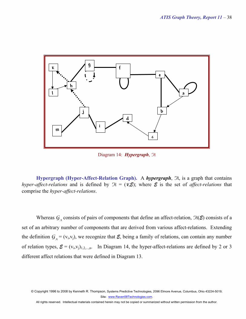
Diagram 14: Hypergraph, H

Hypergraph (Hyper-Affect-Relation Graph). A hypergraph, H, is a graph that contains hyper-affect-relations and is defined by H = (V,E); where E is the set of affect-relations that comprise the hyper-affect-relations.

Whereas GA consists of pairs of components that define an affect-relation, H(E) consists of a

set of an arbitrary number of components that are derived from various affect-relations. Extending

the definition GA = (vi,vj), we recognize that E, being a family of relations, can contain any number

of relation types, E = (vi,vj)1,2,...,n. In Diagram 14, the hyper-affect-relations are defined by 2 or 3

different affect relations that were defined in Diagram 13.

i

h

j d

c

e

b

k

l

m

g

a

f




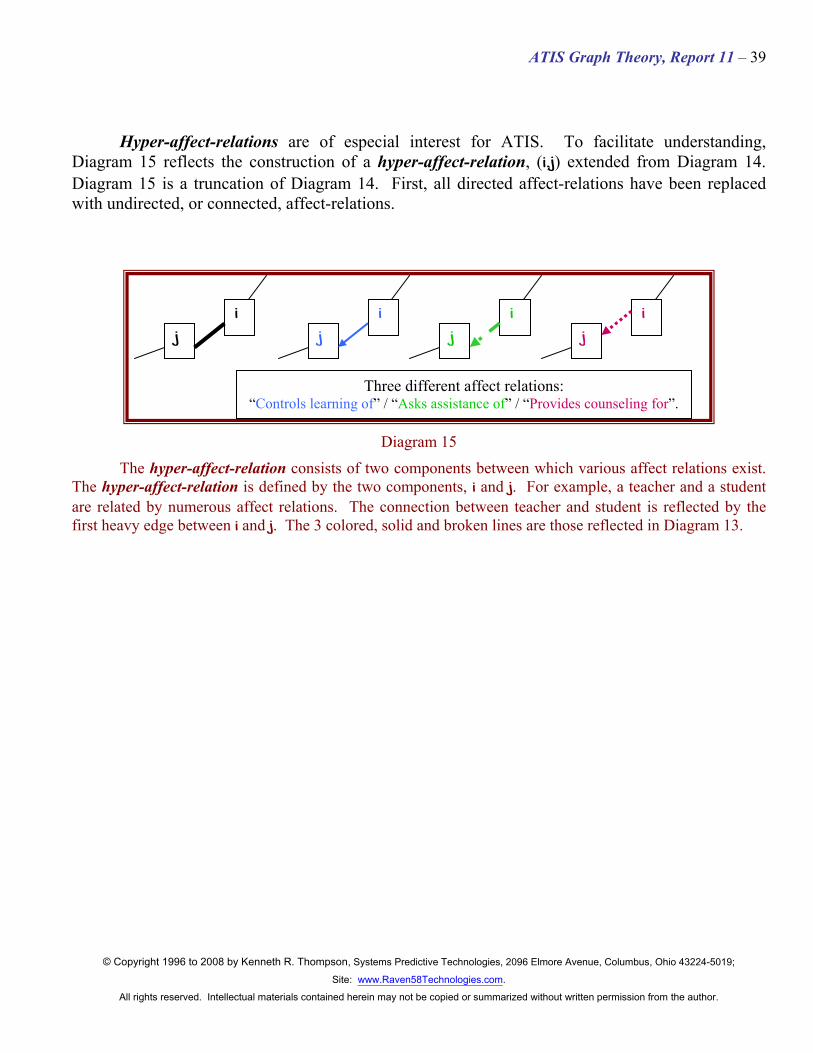
Hyper-affect-relations are of especial interest for ATIS. To facilitate understanding, Diagram 15 reflects the construction of a hyper-affect-relation, (i,j) extended from Diagram 14. Diagram 15 is a truncation of Diagram 14. First, all directed affect-relations have been replaced with undirected, or connected, affect-relations.

Diagram 15

The hyper-affect-relation consists of two components between which various affect relations exist. The hyper-affect-relation is defined by the two components, i and j. For example, a teacher and a student are related by numerous affect relations. The connection between teacher and student is reflected by the first heavy edge between i and j. The 3 colored, solid and broken lines are those reflected in Diagram 13.

ij

i j

ij

i j

Three different affect relations: “Controls learning of” / “Asks assistance of” / “Provides counseling for”.




This report will now continue with the development of ATIS Graph Theory applied to the defining of the ATIS Structural Properties.

In the diagrams, the notation “2; A1-S3” or other similar notation, indicates that there is a path or connection of length 2 from A1 to S3.

It is important to note that every Structural Property is defined in a manner that it is distinctly different from all other Structural Properties. All measures shown in the following examples are distinctly different. While such definitions may not necessarily reflect a desired interpretation, they do reflect distinct attributes of a system and are all closely associated with their initial intent. That is, measures are designed to interpret various attributes of a system, which these definitions do. As such, they must not be changed to reflect some other perspective. If any changes are recommended, they must be considered with respect to the totality of the definitions, and cannot be arbitrarily made on an individual basis. In particular, Active Dependentness and Passive Dependentness definitions are now parallel definitions and reflect the system connectedness of non-adjacent relations. This is an important system attribute that must be measured. Adjacent relations are more than adequately measured through other properties and there is no necessity of defining Dependentness in any other way. Further, it is legitimate to consider that adjacent relations are more than adequately considered by Compactness, Strongness, Unilateralness, Weakness and Wholeness which characterize direct affects, while Dependentness is more properly reflected by relations that have more “substance” to them.

In order to compare the property values side-by-side, the table on the following page is provided. These are the values for the system that is described by the various properties that are defined individually following the table.




Property Values for School System of 14 Components with Relations Shown in Following Charts

Property Count Value

Active Dependence 128.00 paths 338.75

Centrality 61.00 paths 161.44

Compactness 122.00 paths 322.87

Complete Connectedness 4.00 paths 10.59

Complexness 19.00 paths 19.00

Flexibleness log2(64)=6.00 paths 15.88

Heterarchy System 57.00 paths 150.85

Hierarchy System 0.00 paths 0.00

Independence 65.00 paths 172.02

Interdependence log2(15552)=13.92 paths 36.85

Passive Dependence 64.00 paths 169.38

Size 14.00 components 14.00

Strongness log2(248832)=17.92 paths 47.44

Unilateralness 0.00 paths 0.00

Vulnerableness 2.00 paths 5.29

Weakness 15.00 paths 39.70

Wholeness log2(15,552.00)=13.92 paths 36.85




Complexity and Size in a School System

Administrators:

Teachers:

Students:

Affect Relation: Controls Activities of Complexity is the cardinality of the affect-relation set, and Size is the cardinality of the component set. Therefore: M(

XS) = 19.00, and M(

ZS) = 14.00.

Complexness, XS, =df a measure of a partition, Y = (V⊂GO,R⊂G

A), characterized by the number of

affect-relations.

M(XS) =df |Y(R)|

Sizeness, ZS, =df a measure of a partition, Y = (V⊂GO,R⊂G

A), characterized by the number of

components.

M(ZS) =df |Y(V)|

A1 A2

T1 T2 T3 T4

S1 S2 S3 S4

S5 S6 S7 S8




Complexity and Size in a School System

Administrators:

Teachers:

Students:

Affect Relation: Controls Activities of Therefore: M(

XS) = 22.00, 23.00, or 24.00; and M(

ZS) = 17.00.

Complexity and Size Analyses

When considering a school system, a more detailed analysis may be desired than that shown above. For example, whereas all affect-relations are considered the same; i.e., controls activities of, in fact they are quite different. There are several levels of control: Administrator-to-Administrator, Administrator-to-Teacher, Teacher-to-Teacher, Teacher-to-Student, and Student-to-Student. Each of these controls activities of affect-relation can be analyzed as independent affect-relations.

Further, it may be that a greater refinement is desired as reflected in the following graph. In this graph, it is recognized that there may be additional Student-to-Student affect-relations. For this new analysis, complexity and size will have the following values: M(

XS) = 22.00, 23.00 or

24.00; and M(ZS) = 17.00. The previous graph may simply be a truncated version of this graph. It

may be that weighted relations may be required for the previous graph and such will be determined by the analyst. System values are greatly dependent on the expertise of the analyst and intent of the analysis.

A1 A2

T1 T2 T3 T4

S1 S2 S3 S4

S5 S6 S7 S8 S9 S10

S11




Normalization Factor

Most of the definitions that will be used for Structural Properties will require a Normalization Factor in order to have measures that are comparable between systems as well as within a system.

This Normalization Factor accounts for differing sizes between systems and the number of affect-relations that are considered.

Normalization Factor, C, =df [log2(P[Z(SO)]) ÷ n]; for ‘n’ affect relations.

Property-Measure Precision

Property measures are not necessarily as precise as desired and as projected by the theory.

For the Active Dependentness property, the measure is quite accurate since only adjacent components are being measured. However, it is significant to note that in many of the Structural Property definitions any reference to the number of paths related to a property is, at this time, not precise. The reason is that the present state-of-the-art programming will only allow for shortest-path computations between any two components to preclude combinatorial explosion.

However, since all properties will be measured with the same lack of precision, it is considered that, for system-to-system comparisons, the measures will be accurate for their intended purposes until more precise evaluations are possible.




Active Dependentness in a School System

Administrators:

Teachers:

Students:

Affect Relation: Controls Activities of In this system, there are 10 components that Control Activities of other components with respect to Active Dependentness. Since there is only 1 affect-relation and 14 components, then the total possible affect relation paths is P[Z(SO)] = 236,975,181,590; and therefore, C = log2(P[Z(SO)]) l 37. The value is determined by finding the product of the degrees of each initiating component. There are 128 paths related to Active Dependentness. Therefore: M(ADS) l 338.75.

Active dependentness, ADS, =df a partition, Y = (V⊂GO,R⊂GA), characterized by initiating

component affect-relations.

ADS =df Y | ∀vi,vj∈Y(V )∃e∈Y(R)[e = (vi,vj) ∧ dI(v) > 0]

Active dependentness is determined by the initiating-component degrees of the system.

M: Active dependentness measure, M(ADS), =df a measure of initiating component affect-relations.

M(ADS) =df {[Σi=1,…,n(Πj=1,…,mdI(v)j)i] ÷ C} % 100

A1 A2

T1 T2 T3 T4

S1 S2 S3 S4

S5 S6 S7

S8




Centralization in a School System

Administrators:

Teachers:

Students:

Affect Relation: Controls Activities of In this system, there is 1 component that Controls Activities of other components with respect to Centralization. Since there is only 1 affect-relation and 14 components, then the total possible affect relation paths is P[Z(SO)] = 236,975,181,590; and therefore, C = log2(P[Z(SO)]) l 37. There are 61 paths related to Centralization, as can be determined by adding the numbers to the right of the ‘/’.

Therefore: M(CS) l 161.44.

Centralness, CS, =df a partition, Y = (V⊂GO,R⊂GA), characterized by primary-initiating

(independent), non-adjacent component affect-relations.

CS =df Y | ∀vi,vj∈Y(V )∃r(I)(e)∈Y(R)[e = (vi,vj) ⊃ r(I)(e) > 1 ∧ r(T)(e) = 0]

‘r(I)(e)’ is read “The directed-affect-relation, r(e), with respect to the initiating component, I(e)”; and ‘r(T)(e)’ is read “The directed-affect-relation, r(e), with respect to the terminating component,

T(e).”

M: Centralness measure, M(CS), =df a measure of primary-initiating, non-adjacent component affect-relations. Let ‘P’ be the total number of permutations.

M(CS) =df {[Σi=1,…,n (Σj=1,…,m|r(IS)(e) > 1|j)i] ÷ C] % 100

A1 A2

T1 T2 T3 T4

S1 S2 S3 S4

S5 S6 S7 S8

2_A1-S2/1 3_A1-S2/1

2_A1-S1/1

2_A1-S5/1

2_A1-T4/2 This designates the paths of length 2 from ‘A1-T4’. ‘/2’ designates that there are 2 such paths.

3_A1-S8/3 5_A1-S8/1

2_A1-S4/1 4_A1-S4/3

3_A1-T3/1

2_A1-S6/1

2_A1-S3/1 4_A1-S3/1

3_A1-S7/1 2_A1-S7/1 4_A1-S7/1




Compactness in a School System

Administrators:

Teachers:

Students:

Affect Relation: Controls Activities of In this system, there are 10 system components that Control Activities of other components with respect to Compactness. Since there is only 1 affect-relation and 14 components, then the total possible affect relation paths is P[Z(SO)] = 236,975,181,590; and therefore, C = log2(P[Z(SO)]) l 37. There are 122 paths related to Compactness. Therefore: M(CPS) l 322.87.

Compactness, CPS, =df a partition, Y = (V⊂GO,R⊂GA), characterized by initiating, associated

component affect-relations. [Associated components are such that |r(e)| ≥ 1.]

CPS =df Y | ∀vi,vj∈Y(V )∃r(I)(e)∈Y(R)[(e = (vi,vj) ⊃ r(I)(e) ≥ 1)]

‘r(I)(e)’ is read “The directed-affect-relation, r(e), with respect to the initiating component, I(e).”

M: Compactness system measure, M(CPS), =df a measure of initiating, associated component affect-relations. Let ‘P’ be the total number of permutations.

M(CPS) =df {[Σi=1,…,n[log2(Πj=1,…,m|r(I)(e) ≥ 1|j ÷ (|Y(V)|2 - |Y(V)|)]i] ÷ C} % 100

A1 A2

T1 T2 T3 T4

S1 S2 S3 S4

S5 S6 S7 S8

2_A1-S2/ 1 3_A1-S2/1 2_T1-S2/ /1 1_S1-S2/1 1_T2-S2/1

2_A1-S1/1 1_T1-S1/1

2_A1-S5/1 1_T1-S5/1

2_A1-T4/2 1_A2-T4/1 1_T3-T4/1

3_A1-S8/3 5_A1-S8/1 2_A2-S8/1 4_A2-S8/1 2_T3-S8/2 1_T4-S8/1 3_T4-S8/1 1 S4-S8/1

2_A1-S4/1 4_A1-S4/2 3_A2-S4/2 2_T4-S4/2 1_T3-S4/1 3_T3-S4/1 1_S8-S4/1

3_A1-T3/1 1_A1-T3 /1 2_A2-T3/1 1_T4-T3/1

2_A1-S6/1 1_T2-S6/1

2_A1-S3/1 4_A1-S3/1 3_A2-S3/1 2_T4-S3/1 1_T3-S3/1

4_A1-S7/1 3_A1-S7/1 2_A1-S7/1 2_T2-S7/1 1_T3-S7/1 1_S6-S7/1 3_A2-S7/1 2 T4-S7/1

1_A1-A2/1

1_A1-T2/1

1_A1-T1/1




Complete Connectivity in a School System

Administrators:

Teachers:

Students:

Affect Relation: Controls Activities of In this system, there are 2 subsystems and 4 system components that Control Activities of other components with respect to Complete Connectivity. Since there is only 1 affect-relation and 14 components, then the total possible affect relation paths is P[Z(SO)] = 236,975,181,590; and therefore, C = log2(P[Z(SO)]) l 37. There are 4 components related to Complete Connectivity. To analyze this system in more detail, this system can be reduced to a single component for each subsystem to determine the properties of the resulting system. There are 4 paths related to Completeness. Therefore: M(CCS) l 10.59.

Completeness, CCS, =df a partition, Y = (V⊂GO,R⊂GA), characterized by pair-wise directed

associated component affect-relations. [Associated components are such that |r→(e)| ≥ 1.]

CCS =df Y | ∀vi,vj∈Y(V )∃r→(e)∈Y(R)[e = (vi,vj) ∧ e = (vj,vi) ⊃ rd(e) ≥ 1]

‘r→(e)’ is read “The directed-affect-relation, r(e).”

M: Completeness measure, M(CCS), =df a measure of pair-wise directed associated component affect-relations. Let ‘P’ be the total number of permutations.

M(CCS) =df {[Σi=1,…,nlog2(Πj=1,…,m|r→(e) ≥ 1|j)i] ÷ C} % 100

A1 A2

T1 T2 T3 T4

S1 S2 S3 S4

S5 S6 S7 S8





Administrators:

Teachers:

Students:

Therefore: M(CCS) l 85.11.

The previous system has been modified to make only one subsystem that is completely connected as shown by the graph below. In this new system, there are 5 system components that Control Activities of other components with respect to Complete Connectivity. Since there are 14 components, then the total possible affect relation paths is P[Z(SO)] = 236,975,181,590; and therefore, log2(P[Z(SO)]) ≈ 37.786.

This complete connectivity can be reduced to a single component, as shown on the following page, to determine the properties of the resulting system. There are 32 paths related to Completeness in this system.

A1 A2

T1 T2 T3 T4

S1 S2 S3 S4

S5 S6 S7 S8





Administrators:

Teachers:

Students:

Therefore: M(CCS) l 0.00.

The previous system has been modified, as indicated by the bracket, to make only one subsystem that is completely connected. The 5 components have been reduced to one, C1. In this new system, there are 0 system components that Control Activities of other components with respect to Complete Connectivity. Since there are 10 components, then the total possible affect relation paths is P[Z(SO)] = 9,864,090; and therefore, log2(P[Z(SO)]) ≈ 23.234.

One advantage of reducing the system to 0-Connectivity is to determine the effect of the subsystem on the system. This might be of value; e.g., when analyzing a system to see whether the isolation of a subsystem would result in a system behavior that is more desirable. Also, notice that it is irrelevant which component of the isolated subsystem each of A1, A2, S3,and S6 were related to, all that is of concern is that they were related to one of the subsystem components.

A1 A2

T1 T2 T3 T4

S1 S2 S3 S4

S5 S6 S7 S8

C




Analysis Considerations

It is significant to note that the Complete Connectivity of the three previous systems are distinctly different, the first having a measure of 10.59, the second of 85.11, and the third of 0.00.

It is clear from their measures, however, that each would have a different impact on the entire system. Therefore, although subsystems can be reduced to single components, it is important to also determine the effect of each subsystem on the entire system, or to weight the reduced component to reflect their impact.

Analyses that eliminate subsystems are of value, however, to demonstrate the impact of eliminating just such subsystem. For example, in school systems that are experiencing financial difficulties, the first program eliminations are extracurricular activities, art and music, or some other programs that are considered “non-essential.” A system analysis may demonstrate otherwise—or may not and such programs should be cut to conserve finances.




Flexibleness in a School System

Administrators:

Teachers:

Students:

Affect Relation: Controls Activities of In this system, there are 6 components that are accessed by other components with respect to Control Activities of other components with respect to Flexibleness. Since there is only 1 affect-relation and 14 components, then the total possible affect relation paths is P[Z(SO)] = 236,975,181,590; and therefore, C = log2(P[Z(SO)]) l 37. The value is determined by finding the product of the degrees of each component that has 2 or more receiving affect relations. In this case the product is 64, and the log2(64) = 6. There are 6 paths related to Flexibleness. Therefore: M(FS) l 15.88.

Flexibleness, FS, =df a partition, Y = (V⊂GO,R⊂GA), characterized by receiving associated

component affect-relations; such that, the receiving component has receiving-degree greater than 1. [Associated components are such that |r(e)| ≥ 1.]

FS =df Y | ∀vi,vj∈Y(V )∃r(I)(e)∈Y(R)[(e = (vi,vj) ⊃ (r(I)(e) ≥ 1 ∧ d(vj) > 1)]

‘r(I)(e)’ is read “The directed-affect-relation, r(e), with respect to the initiating component, I(e).”

M: Flexibleness measure, M(FS), =Df a measure of receiving associated component affect-relations; such that, the receiving component has degree greater than 1. Let ‘P’ be the total number

of permutations. M(FS) =df {[Σi=1,…,n(Πj=1,…,m[d(Vj)T])i] ÷ C} % 100

A1 A2

T1 T2 T3 T4

S1 S2 S3 S4

S5 S6 S7 S8




Heterarchy-Relatedness in a School System

Administrators:

Teachers:

Students:

Affect Relation: Controls Activities of In this system, there are 6 components that Control Activities of other components with respect to Heterarchy-Relatedness. Since there is only 1 affect-relation and 14 components, then the total possible affect relation paths is P[Z(SO)] = 236,975,181,590; and therefore, C = log2(P[Z(SO)]) l 37. There are 57 paths related to Heterarchy-Relatedness. Therefore: M(HAS) l 150.85.

Heterarchiness, HAS, =df a partition, Y = (V⊂GO,R⊂GA), characterized by associated component

affect-relations that are both initiating and receiving, or leaf associated component affect-relations. [Associated components are such that |r(e)| ≥ 1.]

HAS =df Y | ∀vi,vj∈Y(V )∃r(I,T)(e),r(leaf)(e)∈Y(R)[(e = (vi,vj) ⊃ (r(I,T)(e) ≥ 1 ∨ r(leaf)(e) ≥ 1)]

‘r(I,T)(e)’ is read “The directed-affect-relation, r(e), with respect to an initiating and terminating component, I(e) and T(e); i.e., I(e) = T(e)”; and ‘r(leaf)(e)’ is read “The directed-affect-relation, r(e),

with respect to the leaf component, leaf(e).”

M: Heterarchiness measure, M(HAS), =df a measure of initiating and receiving associated component affect-relations, or receiving associated (leaf) component affect-relations. Let ‘P’ be the total number of permutations.

M(HAS) =df {[Σi=1,…,n(Σj=1,…,m[|rd(I,T)(e) ≥ 1| + |r(T)(e) ≥ 1|]j)i] ÷ C} % 100

A1 A2

T1 T2 T3 T4

S1 S2 S3 S4

S5 S6

S7 S8

2_A1-T4/2 1_A2-T4/1

1_A1-T3/1 3 A1-T3/1

2; A1-S3/1 1; T3-S3/1 4; A1-S3/1 3; A2-S3/1 2; T4-S3/1

2_A1-S7/1 4_A1-S7/1 3_A1-S7/1 3_A2-S7/1 2_T4-S7/1 1_T3-S7/1

2_A1-S4/1 4_A1-S4/2 3_A2-S4/2 2_T4-S4/2 1_T3-S4/1 1_S8-S4/1

3_A1-S8/3 5_A1-S8/1 2_A2-S8/1 4_A2-S8/1 1_T4-S8/1 3_T4-S8/1 2_T3-S8/2 1 S4-S8/1

1_A1-A2/1

1_A1-T1/1

1_A1-T2/1

2_A1-S1/1 1_T1-S1/1

2_A1-S2/1 1_T2-S2/1 3_A1-S2/1 2_T1-S2/1 1_S1-S2/1

2_A1-S5/1 1_T1-S5/1

2_A1-S6/1 1_T2-S6/1




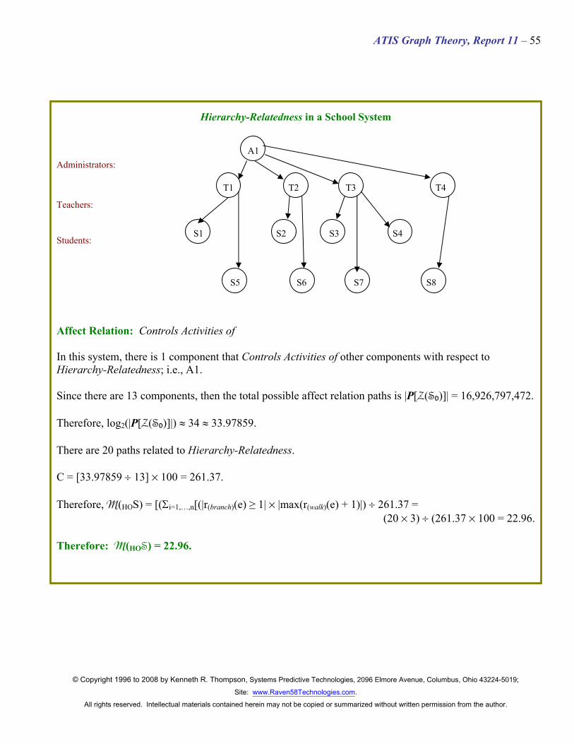
Hierarchy-Relatedness in a School System

Administrators:

Teachers:

Students:

Affect Relation: Controls Activities of In this system, there are no components that Controls Activities of other components with respect to Hierarchy-Relatedness. Since there is only 1 affect-relation and 14 components, then the total possible affect relation paths is P[Z(SO)] = 236,975,181,590; and therefore, C = log2(P[Z(SO)]) l 37. There are 0 paths related to Hierarchy-Relatedness. Although this system has a “root” that could indicate a hierarchy, there are no true levels of connection which are not otherwise connected as a heterarchy; that is there is no “tree” configuration. This structure is not a hierarchy. There are 0 paths related to Hierarchy-Relatedness. Therefore: M(HOS) = 0.00.

Hierarchiness, HOS, =df a partition, Y = (V⊂GO,R⊂GA), characterized by a tree.

HOS =df Y | ∀vi,vj∈Y(V )∃r(tree)(e)v(i),v(j)∈Y(R)[(e = (vi,vj) ⊃ (r(tree)(e)v(i),v(j) = 1)]

‘r(tree)(e)v(i),v(j)’ is read “The directed-affect-relation, r(e), with respect to the tree components, tree(e)”; i.e., for all vi and vj, there is only one directed path.

M: Hierarchiness measure, M(HOS), =df a measure of a tree.

M(HOS) =df {[Σi=1,…,n(Σj=1,…,m[|r(branch)(e) ≥ 1| % |max(r(walk)(e) + 1)|]j)i] ÷ C} % 100

A1 A2

T1 T2 T3 T4

S1 S2 S3 S4

S5 S6 S7 S8




Hierarchy-Relatedness in a School System

Administrators:

Teachers:

Students:

Affect Relation: Controls Activities of In this system, there is 1 component that Controls Activities of other components with respect to Hierarchy-Relatedness; i.e., A1. Since there are 13 components, then the total possible affect relation paths is |P[Z(SO)]| = 16,926,797,472. Therefore, log2(|P[Z(SO)]|) l 34 l 33.97859. There are 20 paths related to Hierarchy-Relatedness. C = [33.97859 ÷ 13] % 100 = 261.37. Therefore, M(HOS) = [(Σi=1,…,n[(|r(branch)(e) ≥ 1| % |max(r(walk)(e) + 1)|) ÷ 261.37 =

(20 % 3) ÷ (261.37 % 100 = 22.96. Therefore: M(HOS) = 22.96.

A1

T1 T2 T3 T4 S1 S2 S3 S4

S5 S6 S7 S8




Independentness in a School System

Administrators:

Teachers:

Students:

Affect Relation: Controls Activities of In this system, there is 1 component that Controls Activities of other components with respect to Independentness. Since there is only 1 affect-relation and 14 components, then the total possible affect relation paths is P[Z(SO)] = 236,975,181,590; and therefore, C = log2(P[Z(SO)]) l 37. There are 64 paths related to Independentness. Therefore: M(IS) l 172.02

Independentness, IS, =df a partition, Y = (V⊂GO,R⊂GA), characterized by primary-initiating

associated component affect-relations. [Associated components are such that |r(e)| ≥ 1.]

IS =df Y | ∀vi,vj∈Y(V )∃r(I)(e)∈Y(R)[e = (vi,vj) ⊃ r(I)(e) ≥ 1 ∧ r(T)(e) = 0]

‘r(I)(e)’ is read “The directed-affect-relation, r(e), with respect to the initiating component, I(e)”; and ‘r(T)(e)’ is read “The directed-affect-relation, r(e), with respect to the terminating component, T(e)”

M: Independentness measure, M(IS), =df a measure of primary-initiating component affect-relations. Let ‘P’ be the total number of permutations.

M(IS) =df {[Σi=1,…,n(Σj=1,…,m|r(PI)(e) ≥ 1|j)i] ÷ C} % 100

A1 A2

T1 T2 T3 T4

S1 S2 S3 S4

S5 S6 S7 S8

39 paths for A2, T4, T3, S3, S4, & S8 (from the right)

9 paths for T3, S3, S4, S7 (from right), & S8

16 paths for T1, T2, S1, S2, S5, S6, & S7 (from the left)




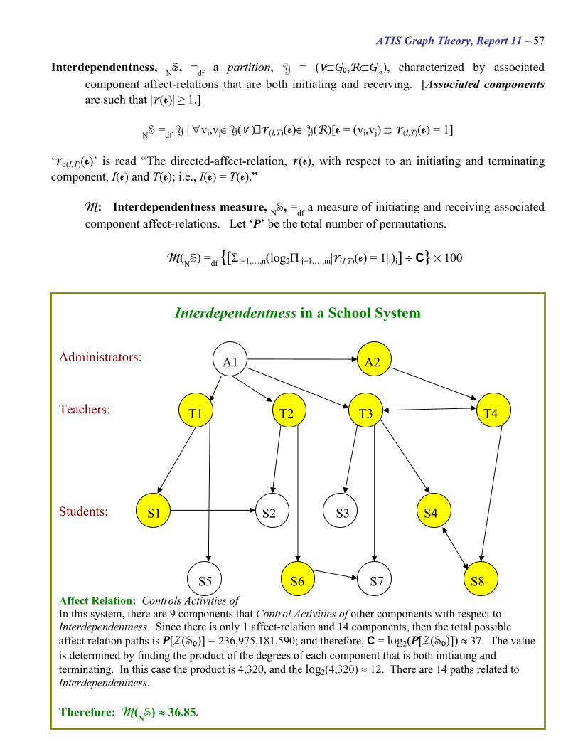
Interdependentness in a School System

Administrators:

Teachers:

Students:

Affect Relation: Controls Activities of In this system, there are 9 components that Control Activities of other components with respect to Interdependentness. Since there is only 1 affect-relation and 14 components, then the total possible affect relation paths is P[Z(SO)] = 236,975,181,590; and therefore, C = log2(P[Z(SO)]) l 37. The value is determined by finding the product of the degrees of each component that is both initiating and terminating. In this case the product is 4,320, and the log2(4,320) ≈ 12. There are 14 paths related to Interdependentness. Therefore: M(NS) l 36.85.

Interdependentness, NS, =df a partition, Y = (V⊂GO,R⊂GA), characterized by associated

component affect-relations that are both initiating and receiving. [Associated components are such that |r(e)| ≥ 1.]

NS =df Y | ∀vi,vj∈Y(V )∃r(I,T)(e)∈Y(R)[e = (vi,vj) ⊃ r(I,T)(e) = 1]

‘rd(I,T)(e)’ is read “The directed-affect-relation, r(e), with respect to an initiating and terminating component, I(e) and T(e); i.e., I(e) = T(e).”

M: Interdependentness measure, NS, =df a measure of initiating and receiving associated component affect-relations. Let ‘P’ be the total number of permutations.

M(NS) =df {[Σi=1,…,n(log2Π j=1,…,m|r(I,T)(e) = 1|j)i] ÷ C} % 100

A1 A2

T1 T2 T3 T4

S1 S2 S3 S4

S5 S6 S7 S8




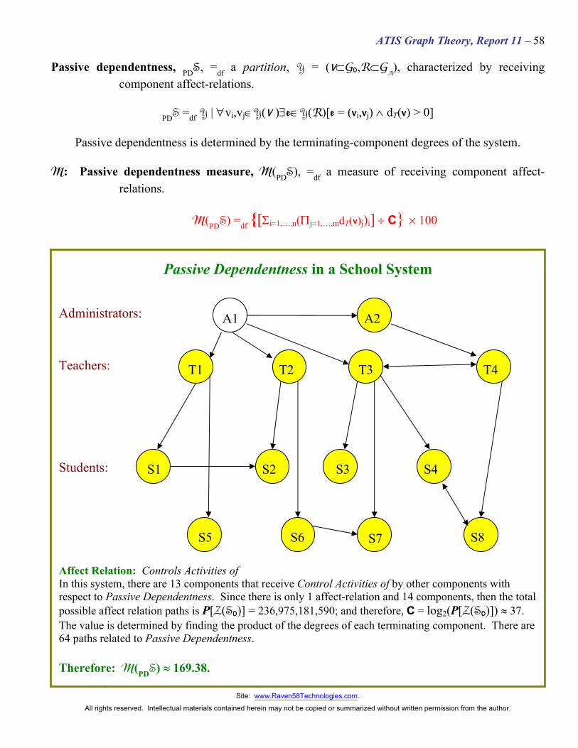
Passive Dependentness in a School System

Administrators:

Teachers:

Students:

Affect Relation: Controls Activities of In this system, there are 13 components that receive Control Activities of by other components with respect to Passive Dependentness. Since there is only 1 affect-relation and 14 components, then the total possible affect relation paths is P[Z(SO)] = 236,975,181,590; and therefore, C = log2(P[Z(SO)]) l 37. The value is determined by finding the product of the degrees of each terminating component. There are 64 paths related to Passive Dependentness. Therefore: M(PDS) l 169.38.

Passive dependentness, PDS, =df a partition, Y = (V⊂GO,R⊂GA), characterized by receiving

component affect-relations.

PDS =df Y | ∀vi,vj∈Y(V )∃e∈Y(R)[e = (vi,vj) ∧ dT(v) > 0]

Passive dependentness is determined by the terminating-component degrees of the system.

M: Passive dependentness measure, M(PDS), =df a measure of receiving component affect-relations.

M(PDS) =df {[Σi=1,…,n(Πj=1,…,mdT(v)j)i] ÷ C} % 100

A1 A2

T1 T2 T3 T4

S1 S2 S3 S4

S5 S6 S8 S7




Strongness in a School System

Administrators:

Teachers:

Students:

Affect Relation: Controls Activities of In this system, there are 14 components that Control Activities of other components with respect to Strongness since all components are connected and numerous components are directed adjacent or non-adjacent connected. Since there is only 1 affect-relation and 14 components, then the total possible affect relation paths is P[Z(SO)] = 236,975,181,590; and therefore, C = log2(P[Z(SO)]) l 37. The product of the component degrees is 248,832, with a log2|248,832| l 18. There are 18 paths related to Independentness. Therefore: M(SS) l 47.44.

Strongness, SS, =df a partition, Y = (V⊂GO,R⊂GA), characterized by connected associated

components. [Associated components are such that |r(e)| ≥ 1.]

SS =df Y | ∀vi,vj∈Y(V )∃r→(e)∈Y(R)[e = (vi,vj)∈R]


M: Strongness measure, SS, =df a measure of the degree of connected components. Let ‘P’ be the total number of permutations.

M(SS) =df {[log2Σi=1,…,n(Π j=1,…,md(vj))i] ÷ C} % 100

A1 A2

T1 T2 T3 T4

S1 S2 S3 S4

S5 S6 S7 S8




Unilateralness (Chains) in a School System

Administrators:

Teachers:

Students:

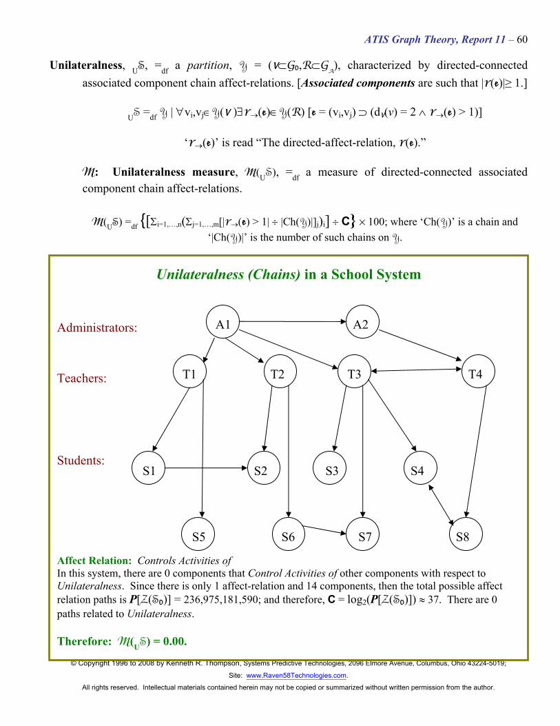
Affect Relation: Controls Activities of In this system, there are 0 components that Control Activities of other components with respect to Unilateralness. Since there is only 1 affect-relation and 14 components, then the total possible affect relation paths is P[Z(SO)] = 236,975,181,590; and therefore, C = log2(P[Z(SO)]) l 37. There are 0 paths related to Unilateralness. Therefore: M(US) = 0.00.

Unilateralness, US, =df a partition, Y = (V⊂GO,R⊂GA), characterized by directed-connected

associated component chain affect-relations. [Associated components are such that |r(e)|≥ 1.]

US =df Y | ∀vi,vj∈Y(V )∃r→(e)∈Y(R) [e = (vi,vj) ⊃ (dV(v) = 2 ∧ r→(e) > 1)]


M: Unilateralness measure, M(US), =df a measure of directed-connected associated component chain affect-relations.

M(US) =df {[Σi=1,…,n(Σj=1,…,m[|r→(e) > 1| ÷ |Ch(Y)|]j)i] ÷ C} % 100; where ‘Ch(Y)’ is a chain and ‘|Ch(Y)|’ is the number of such chains on Y.

A1 A2

T1 T2 T3 T4

S1 S2 S3 S4

S5 S6 S7 S8




Unilateralness (Chains) in a School System

Administrators:

Teachers:

Students:

Affect Relation: Controls Activities of Therefore: M(US) = 14.11.

In the system shown below which has been modified from the one above, there are 12 components that Control Activities of other components with respect to Unilateralness. Since there are 14 components, then the total possible affect relation paths is P[Z(SO)] = 236,975,181,590; and therefore, log2(P[Z(SO)]) l 37.786.

For these 12 components there are 5 different chains. However, only 3 of these chains are

relevant to this measure; i.e., those with 2 or more paths—the blue and orange chains are not relevant for this measure. There are 16 paths related to the relevant chains.

A1 A2

T1 T2 T3 T4

S1 S2 S3 S4

S5 S6 S7 S8




Vulnerableness in a School System

Administrators:

Teachers:

Students:

Affect Relation: Controls Activities of In this system, there are there are 2 components that Control Activities of other components with respect to Vulnerableness. Since there is only 1 affect-relation and 14 components, then the total possible affect relation paths is P[Z(SO)] = 236,975,181,590; and therefore, C = log2(P[Z(SO)]) l 37. There are 2 paths related to Vulnerableness. Therefore: M(VS) l 5.29.

Vulnerableness, VS, =df a partition, Y = (V⊂GO,R⊂GA), characterized by leaf affect-

relations.

VS =df Y | ∀vi,vj∈Y(V )∃r(leaf)(e)∈Y(R) [e = (vi,vj) ⊃ r(leaf)(e) = 1)]

‘r(leaf)(e)’ is read “The directed-affect-relation, r(e), with respect to the leaf component, leaf(e)”

M: Vulnerableness measure, VS, =df a measure of directed-connected adjacent terminating component affect-relations. Let ‘P’ be the total number of permutations.

M(VS) =df {[Σi=1,…,n(Σj=1,…,m|r(leaf)(e) = 1|j)i] ÷ C} % 100

A1 A2

T1 T2 T3 T4

S1 S2 S3 S4

S5 S6 S7 S8

1_T3-S3/1

1_T1-S5/1




Weakness in a School System

Administrators:

Teachers:

Students:

Affect Relation: Controls Activities of In this system, there are there are 13 components that Control Activities of other components with respect to Weakness. Since there is only 1 affect-relation and 14 components, then the total possible affect relation paths is P[Z(SO)] = 236,975,181,590; and therefore, C = log2(P[Z(SO)]) l 37. There are 15 paths related to Weakness. Therefore: M(WCS) l 39.70.

Weakness, WKS, =df a partition, Y = (V⊂GO,R⊂GA), characterized by adjacent connected affect-

relations that are not directed-connected.

WKS =df Y | ∀vi,vj∈Y(V )∃r~→(e)∈Y(R)[e = (vi,vj) ⊃ (r~→(e) = 1)]

‘r~→(e)’ is read “The non-directed-affect-relation, r(e).”

M: Weakness measure, WKS, =df a measure of associated connected affect-relations that are not directed-connected, and leaf affect-relations. Let ‘P’ be the total number of permutations.

M(WKS) =df {[Σi=1,…,n(Σj=1,…,m|r~→(e) = 1|j)i] ÷ C} % 100

A1 A2

T1 T2 T3 T4

S1 S2 S3 S4

S5 S6 S7 S8

1_A2-A1/1

1_T1-A1/1

1_T2-A1/1 1_T3-A1/1

1_T4-A2/1

1_S1-T1/1 1_S2-T2/1 1_S2-S1/1

1_S3-T3/1

1_S4-T3/1

1_S5-T1/1 1_S6-T2/1 1; S7-S6/1

1; S7-T3/1 1_S8-T4/1




Wholeness in a School System

Administrators:

Teachers:

Students:

Affect Relation: Controls Activities of In this system, there is 1 component that Controls Activities of other components with respect to Wholeness. Since there is only 1 affect-relation and 14 components, then the total possible affect relation paths is P[Z(SO)] = 236,975,181,590; and therefore, C = log2(P[Z(SO)]) l 37. The product of the component degrees not including the wholly-connected component is 17,280, with a log2|17,280| l 14. There are 14 paths related to Independentness. Therefore: M(WS) l 36.85.

Wholeness, WS, =df a partition, Y = (V⊂GO,R⊂GA

), characterized by associated directed-connected affect-relations from components directed-connected to all other components, other than primary-initiating components. [Associated components are such that |r(e)| ≥ 1.]

WS =df Y | ∃vi∀vj∈Y(V )∃rd(e)∈Y(R) [e = (vi,vj) ⊃ rd(e) ≥ 1)]


M: Wholeness measure, M(WA), =df a measure of associated directed-connected affect-relations from components connected to all other components. Let ‘P’ be the total number of permutations.

M(WS) =df {[Σi=1,…,n(Σj=1,…,m[|r→(e)| ÷ |W(v)|]j)i] ÷ C} % 100; Where j does not include W(v), and where W(v) are the wholly-connected components, and |W(v) = 0| = 1.

A1 A2

T1 T2 T3 T4

S1 S2 S3 S4

S5 S6 S7 S8

Date post:	19-May-2018
Category:	Documents
Upload:	hoangnhu
View:	218 times
Download:	1 times

ATIS Graph Theory - Indiana University Bloomington · ATIS Graph Theory ATIS Graph Theory is...

Documents