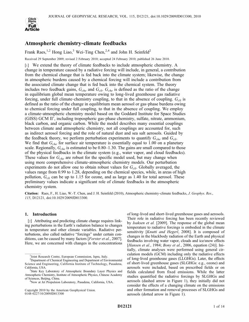
ClickHere

for

FullArticle

Atmospheric chemistry‐climate feedbacks

Frank Raes,1,2 Hong Liao,3 Wei‐Ting Chen,2,4 and John H. Seinfeld2

Received 29 September 2009; revised 2 February 2010; accepted 24 February 2010; published 26 June 2010.

[1] We extend the theory of climate feedbacks to include atmospheric chemistry. Achange in temperature caused by a radiative forcing will include, in general, a contributionfrom the chemical change that is fed back into the climate system; likewise, the changein atmospheric burdens caused by a chemical forcing will include a contribution fromthe associated climate change that is fed back into the chemical system. The theoryincludes two feedback gains, Gche and Gcli. Gche is defined as the ratio of the changein equilibrium global mean temperature owing to long‐lived greenhouse gas radiativeforcing, under full climate‐chemistry coupling, to that in the absence of coupling. Gcli isdefined as the ratio of the change in equilibrium mean aerosol or gas‐phase burdens owingto chemical forcing under full coupling, to that in the absence of coupling. We employa climate‐atmospheric chemistry model based on the Goddard Institute for Space Studies(GISS) GCM II’, including tropospheric gas‐phase chemistry, sulfate, nitrate, ammonium,black carbon, and organic carbon. While the model describes many essential couplingsbetween climate and atmospheric chemistry, not all couplings are accounted for, suchas indirect aerosol forcing and the role of natural dust and sea salt aerosols. Guided bythe feedback theory, we perform perturbation experiments to quantify Gche and Gcli.We find that Gche for surface air temperature is essentially equal to 1.00 on a planetaryscale. Regionally, Gche is estimated to be 0.80–1.30. The gains are small compared to thoseof the physical feedbacks in the climate system (e.g., water vapor, and cloud feedbacks).These values for Gche are robust for the specific model used, but may change whenusing more comprehensive climate‐atmospheric chemistry models. Our perturbationexperiments do not allow one to obtain robust values for Gcli. Globally averaged, thevalues range from 0.99 to 1.28, depending on the chemical species, while, in areas of highpollution, Gcli can be up to 1.15 for ozone, and as large as 1.40 for total aerosol. Thesepreliminary values indicate a significant role of climate feedbacks in the atmosphericchemistry system.

Citation: Raes, F., H. Liao, W.-T. Chen, and J. H. Seinfeld (2010), Atmospheric chemistry‐climate feedbacks, J. Geophys. Res.,115, D12121, doi:10.1029/2009JD013300.

1. Introduction

[2] Attributing and predicting climate change requires link-ing perturbations in the Earth’s radiation balance to changesin temperature and other climate variables. Radiative per-turbations, also called radiative “forcings” under certain con-ditions, can be caused by many factors [Forster et al., 2007].Here, we are concerned with changes in the concentrations

of long‐lived and short‐lived greenhouse gases and aerosols.Their role in radiative forcing has been recently reviewedby Isaksen et al. [2009]. The response of the global meantemperature to radiative forcings is embodied in the climatesensitivity [Knutti and Hegerl, 2008]. It is composed ofchanges in the blackbody radiation of the Earth and physicalfeedbacks involving water vapor, clouds and ice/snow effects[Hansen et al., 1984; Bony et al., 2006, equation (24)]. Ini-tially, climate analyses were performed using general cir-culation models (GCM) including only the radiative effectsof long‐lived greenhouse gases (LLGHGs). Later, the effectsof short‐lived greenhouse gases (SLGHGs: e.g., ozone) andaerosols were included, based on prescribed fields or onfields calculated from fixed emissions. While the latterstudies quantified the radiative forcings by SLGHGs andaerosols (dashed arrow in Figure 1), they initially did notconsider the effects of a changing climate on the emissionsand other formation and removal processes of SLGHGs andaerosols (dotted arrow in Figure 1).

1Joint Research Centre, European Commission, Ispra, Italy.2Department of Chemical Engineering and Department of Environmental

Science and Engineering, California Institute of Technology, Pasadena,California, USA.

3State Key Laboratory of Atmospheric Boundary Layer Physics andAtmospheric Chemistry, Institute of Atmospheric Physics, Chinese Academyof Sciences, Beijing, China.

4Now at Jet Propulsion Laboratory, Pasadena, California, USA.

Copyright 2010 by the American Geophysical Union.0148‐0227/10/2009JD013300

JOURNAL OF GEOPHYSICAL RESEARCH, VOL. 115, D12121, doi:10.1029/2009JD013300, 2010

D12121 1 of 14

[3] Atmospheric chemistry developed initially in parallelwith climate science, with its early applications to airpollution. Following the thinking in climate sciences, wewill consider perturbations in the formation, transforma-tion, and removal of atmospheric species, and describe theresponse of the chemical composition of the atmosphere tosuch perturbations through an atmospheric chemistry sen-sitivity. This sensitivity includes chemical feedbacks, suchas those in the CH4, CO, OH system [Isaksen and Hov,1987]. Because of the many interacting atmospheric spe-cies, the atmospheric chemistry sensitivity is not a singlevalue. This sensitivity should, in fact, be expressed in termsof the Jacobian matrix of the atmospheric chemistry sys-tem [Prather, 1994], through which the change of the con-centration of a single species can be calculated as a functionof the rates of change (including, e.g., emission changes)of all other species. Atmospheric chemistry and air pollu-tion studies are typically performed with atmosphericchemical transport models (CTMs), with prescribed climate.For example, in studies that evaluate the effect of reducingemissions of air pollutants over, say, the next 30 years, aconstant climate is typically assumed. Isaksen et al. [2009]reviewed studies of the effect of air pollution emissionchanges in a future climate as compared to that at present(dotted arrow in Figure 1); however, in those studies, theeffects of the changing atmospheric composition on theclimate itself are usually not considered (dashed arrow inFigure 1).[4] Climate models have become increasingly sophisti-

cated, although not yet comprehensive in allowing forcomplete two‐way coupling between climate and chemicalprocesses. The review by Isaksen et al. [2009], dealing withclimate‐chemistry interactions, largely divides the workinto, on one hand, the impacts of changes in atmospheric

composition on climate, and, on the other hand, impacts ofclimate change on atmospheric composition. Many of thestudies reviewed note the existence of feedbacks but, infact, refer only to a one‐way coupling between climate andatmospheric chemistry, or vice versa. Two recent papersmore systematically address the feedback effects resultingfrom two‐way coupling. Liao et al. [2009] approach theclimate‐atmospheric chemistry system by studying theproduction, transformation, and removal of troposphericozone and aerosols fully coupled to the evolving climate.GCM simulations with and without full coupling showsignificant differences in the predicted levels of equilibriumglobal mean temperature and global and regional levels ofozone and aerosols. Their study did not include aerosol‐cloud interactions: the aerosol indirect effect. Unger et al.[2009] looked, in particular, at the effect of coupling ofozone and aerosols with cloud microphysical processes.They also found significant effects of full coupling onlevels of air pollutants.[5] The above mentioned review and studies, while giv-

ing an exhaustive overview of processes that couple cli-mate with atmospheric chemistry, indicate that atmosphericchemistry research would benefit from a consistent frame-work for discussing, quantifying and comparing feedbacksin the climate‐atmospheric chemistry system. We propose aframework based on Figure 1. Although we deal essentiallywith one feedback loop within the fully coupled system, wecan, and will, throughout this paper, maintain two points ofview. The first is that of the climatologist, who is interestedin how the presence of chemically active species in theatmosphere leads to feedbacks in the climate system, in thesame way as, for example, water vapor leads to feedbacksand enhances climate sensitivity. As such we will speakabout the atmospheric chemistry feedback in the climatesystem. The second view is that of the atmospheric chemist,who is interested how climate leads to feedbacks in theatmospheric chemistry system that affect the relationshipbetween emissions and burdens of chemical components,or, generally speaking, the atmospheric chemistry sensitivity.We will speak about the climate feedback in the atmosphericchemistry system. Together these constitute the atmosphericchemistry‐climate feedbacks referred to in the title of thispaper.[6] The working of feedbacks in the coupled climate‐

atmospheric chemistry system can be illustrated with aconcrete example. Consider a scenario in which both climateand atmospheric chemistry are at steady state and globalSO2 emissions were to be suddenly reduced. Reduction inSO2 emissions leads immediately to a reduction in the for-mation of airborne sulfate aerosol. A global reduction insulfate aerosol leads to a decrease in the negative radiativeforcing associated with sulfate aerosol. As the Earth warmsin response to the aerosol perturbation, the hydrologicalcycle adjusts such that the removal of sulfate aerosol byprecipitation is, say, increased. At this point the feedbackloop is closed. The additional decrease in sulfate aerosol,beyond that resulting from the original SO2 reduction, fur-ther warms the system, and so on, until a new steady stateis achieved. The eventual new steady state results fromthe two‐way coupling between climate and atmosphericchemistry. The atmospheric chemistry sensitivity, linkingthe SO2 emission reduction to a change in sulfate burden,

Figure 1. Box diagram of the fully coupled climate‐atmospheric chemistry system, where lcli and lche are theclimate and atmospheric chemistry sensitivities, respec-tively, c10 is a coupling factor used in describing the effectof climate on atmospheric chemistry, and c01 is a couplingfactor describing the effect of atmospheric chemistry onclimate. We are interested in how radiative and chemicalperturbations/forcings, DR0 f and DR1 f , affect steady stateclimate and atmospheric chemistry, DTss and DCss.

RAES ET AL.: CHEMISTRY‐CLIMATE FEEDBACK D12121D12121

2 of 14

as well as the climate sensitivity, linking the sulfate forcingto a temperature change, are each changed by the feedbackwithin the fully coupled system. The question is: by howmuch?[7] Hence, at a general level, we seek to evaluate the

extent to which the presence of chemically active speciesin the atmosphere leads to feedbacks in the climate sys-tem. At the same time, we will evaluate how climate pro-cesses lead to feedbacks in the atmospheric chemistrysystem. At a more practical level, we want know whatdegree of sophistication is needed to perform integratedclimate change and air pollution analysis. Ideally, the besttool is a fully coupled climate‐atmospheric chemistrymodel, with comprehensive treatment of all important cli-mate and chemical processes. However, even the mostcomprehensive current coupled models require the maxi-mum computing capacity available in, for example, a typ-ical research or meteorological center. They are thereforenot practical for evaluating multiple scenarios needed inthe analysis of combined climate change and air pollutionmitigation options. Before making the case that fully cou-pled models are indeed necessary, it is of interest to eval-uate the importance of coupling, i.e., to quantify the strengthof the atmospheric chemistry‐climate feedbacks.[8] In this work, we use Figure 1 as a framework to

study more systematically the full coupling between climateand atmospheric chemistry and the resulting feedbacks. Indoing so, we use the traditional analysis of climate sensi-tivity and feedbacks [e.g., Hansen et al., 1984; Bony et al.,2006; Schwartz, 2007; Roe and Baker, 2007; Roe, 2009]and extend it to include atmospheric chemistry sensitivityand feedbacks. In section 2, we describe this frameworktheoretically, and in section 3, guided by the framework, weperform a number of perturbation experiments with a fullycoupled climate‐atmospheric chemistry GCM. This allowsus to study the effect of full coupling on both global climateand levels of air pollutants. In section 4, we focus on theclimate system, quantify the atmospheric chemistry feed-back and compare it with the known physical feedbacksdue to changing water vapor, lapse rate, albedo, and clouds.

2. Coupling the Climate and AtmosphericChemistry Systems: Theoretical Framework

[9] In order to illustrate the coupling between climateand atmospheric chemistry, it is sufficient to describe thecoupled system in terms of the Earth’s global mean tem-perature, T, and the concentration of a single genericchemical component, C.[10] The basic dynamic equation for T follows from the

overall planetary energy balance,

cdT

dt¼ S0

4ð1� AðT ;CÞÞ � "ðT ;CÞ�T 4; ð1Þ

where c is the effective heat capacity of the atmosphere‐ocean system, and cdT is the change in the heat contentof the system arising from an imbalance between incomingand outgoing radiation. S0 is the solar constant and s theStefan‐Boltzmann constant. A(T,C) is the planetary albedo,determined partly by cloudiness, aerosols, and the presence

of snow and ice, each of which depends in a complexmanner on T and C. "(T,C) is the planetary longwaveemissivity, which depends on the level of LLGHGs in theatmosphere, including water vapor and SLGHGs, such astropospheric ozone, which themselves depend on T and C.[11] The dynamic equation for C follows from the global

material balance of a species,

dC

dt¼ EðT ;CÞ � DðT ;CÞ þ RX ðT ;CÞ: ð2Þ

E(T,C) and D(T,C) are the emission and physical removalrates, respectively, of the chemical component. The latterincludes dry and wet deposition rates, which are dependenton the concentration of the species and on climatic condi-tions. Emissions of one species could, in principle, depend onthe concentration of other chemical components. RX(T,C)describes the net rate of chemical production of the species.[12] At this stage we have introduced two ways to describe

the coupling between climate and atmospheric chemistry:the set of coupled differential equations (1) and (2), for Tand C, respectively, and the “box diagram” in Figure 1,with its sensitivity parameters l and coupling factors c. It isuseful to show how these two descriptions relate to oneanother, as it will help us in the discussion of feedbacks.

2.1. Perturbation Analysis

[13] We can express equations (1) and (2) in terms ofradiative and chemical imbalances as follows,

cdT

dt¼ R0ðT ;CÞ ¼ the radiative imbalance ðW m�2Þ ð3aÞ

dC

dt¼ R1ðT ;CÞ ¼ the chemical imbalance ð�g m�3 s�1Þ: ð3bÞ

Starting from a steady state, Ri(Tss,C ss) = 0 (i = 0,1), and

applying sustained perturbations, DR0 f and DR1 f (i.e.,radiative and chemical forcings, respectively), the climate‐atmospheric chemistry system will act to restore radiativeand chemical equilibrium. It will relax to a new steady stateat which incoming and outgoing energy fluxes and sourcesand sinks of chemical species are again in balance: Ri (T

ss +DT ss, C ss + DC ss) = 0 (i = 0,1). At any moment during therelaxation, the change of the imbalances can be written asfollows:

�Ri ¼ @Ri

@T

����C

�T þ @Ri

@C

����T

�C i ¼ 0; 1: ð4Þ

Integrating between the start of the perturbation (when Ri =DRif ) and reaching the new steady state (when Ri = 0) yields

Z0

DRif

�Ri ¼ZTssþDTss

Tss

@Ri

@T

����C

�T þZCssþDCss

Css

@Ri

@C

����T

�C i ¼ 0; 1: ð5Þ

Assuming linear behavior in the vicinity of the steady states,it follows that

DRif¼ � @Ri

@T

����C

DTss � @Ri

@C

����T

DCss i ¼ 0; 1 ð6Þ

RAES ET AL.: CHEMISTRY‐CLIMATE FEEDBACK D12121D12121

3 of 14

or, in matrix form,

DR0f

DR1f

" #¼�

@R0

@T

����C

@R0

@C

����T

@R1

@T

����C

@R1

@C

����T

26664

37775 DTss

DCss

� �¼ �J

DTss

DCss

� �: ð7Þ

J, the Jacobian of the coupled system described byequations (1) and (2), contains the complete sensitivity infor-mation. The result as expressed in equation (7) is a standardone in systems and control theory [Athans and Falb, 1966].

2.2. Feedback Analysis

[14] Figure 1 is a “box diagram,” used in traditional feed-back analysis. It shows (see Appendix A) that the changein temperature, caused by a radiative forcing DR0 f , will bea result from that forcing, plus a contribution from thechemical change that also results and that is fed back intothe climate system. Hence,

DT ss ¼ �cliðDR0 f þ c01DC ssÞ; ð8aÞ

where lcli is the sensitivity parameter of the climate system,and c01 is the factor that represents one‐way coupling ofchemical change with climate. Similarly, for the change inthe concentration of a chemical compound, caused by achemical forcing DR1f, we can write

DC ss ¼ �cheðDR1 f þ c10DT ssÞ; ð8bÞ

where lche is the sensitivity parameter of the atmosphericchemistry system, and c10 is the factor that represents one‐way coupling of climate change on atmospheric chemistry.[15] Solving (8a) and (8b) for DR0 f and DR1 f , and writ-

ing in matrix notation yields

DR0 f

DR1 f

� �¼ ��1

cli �c01�c10 ��1

che

� �DT ss

DCss

� �: ð9Þ

Comparing (7) with (9) gives an immediate interpretation ofthe elements in the Jacobian, of which we will make uselater.[16] Inverting equation (9) yields

DT ss

DC ss

� �¼ �cli�che

1� �cli�chec01c10

��1che c01

c10 ��1cli

� �DR0 f

DR1 f

� �: ð10Þ

2.3. Assessing the Atmospheric Chemistry Feedbackin the Climate System

[17] From equation (10) it follows that

DT ss ¼ �cli

1� �cli�chec01c10ðDR0 f þ �chec01DR1 f Þ: ð11Þ

This shows that in the fully, i.e., two‐way, coupled climate‐atmospheric chemistry system, the global mean temperatureis, in principle, sensitive to both radiative and chemical for-cings. The effects of both forcings are additive, but that holdsonly as long as it is justified to assume linear behavior (seeequations (6) and (8)), which must be checked subsequently.

[18] If there is no full coupling between climate andchemistry (c01 = 0 or c10 = 0 or c01 = c10 = 0), equation (11)becomes

DTssun ¼ �cliðDR0 f þ �chec01DR1 f Þ: ð12Þ

Comparing (11) and (12) shows how, because of full cou-pling with atmospheric chemistry, the climate sensitivityparameter changes,

�cli ������!coupling� ¼ �cli

1� �cli�chec01c10; ð13Þ

where l is the climate sensitivity parameter of the coupledsystem. According to the feedback analysis (see equation (A4)),lchec01c10 has the significance of a feedback parameter, andcan be termed the atmospheric chemistry feedback parameter,cche,

cche ¼ �chec01c10: ð14Þ

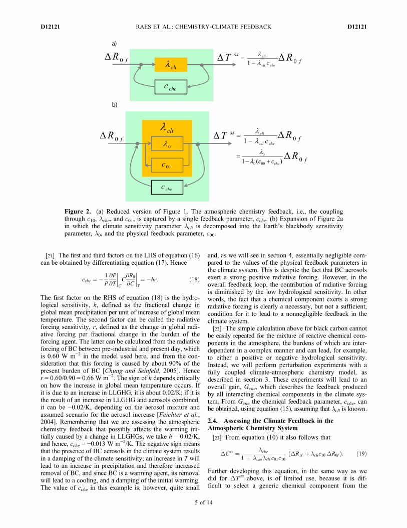
In fact, if we are interested only in radiative perturbations(DR1f = 0), but still want to describe the feedback dueto atmospheric chemistry, Figure 1 can be simplified intoFigure 2.[19] Following equation (A5), the gain Gche of the sys-

tem, i.e., the ratio of output of the coupled system to theoutput of the uncoupled system, can be calculated as theratio of equations (11) and (12),

Gche ¼ DTss

DTssun

¼ 1

1 � �cli cche: ð15Þ

If cche < 0, then Gche < 1 and atmospheric chemistry willdampen the climate sensitivity; if cche > 0, then Gche > 1and it will amplify the climate sensitivity.[20] As shown in equation (14), the atmospheric chemis-

try feedback is composed of three factors, and using thecomparison of the matrices in (7) and (9), it can be writtenmore explicitly as

cche ¼ �chec01c10 ¼ � @R1

@C

����T

� ��1@R0

@C

����T

@R1

@T

����C

ðW m�2=KÞ:

ð16Þ

Each of the three factors can determine the sign and themagnitude of the atmospheric chemistry feedback. What thismeans can be illustrated by considering a simple system,consisting of nonreactive black carbon (BC) aerosols only.In this case, equation (2) becomes

dC

dt¼ E � �ðTÞC ¼ R1ðTÞ; ð17Þ

where C is the global burden of BC, E its global emissionsrate, and b(T) its globally average removal rate. The latter istaken to be proportional to the precipitation rate P, which isknown to be dependent on the global mean temperature T:b(T) = aP(T).

RAES ET AL.: CHEMISTRY‐CLIMATE FEEDBACK D12121D12121

4 of 14

[21] The first and third factors on the LHS of equation (16)can be obtained by differentiating equation (17). Hence

cche ¼ � 1

P

@P

@T

����C

C@R0

@C

����T

¼ �hr: ð18Þ

The first factor on the RHS of equation (18) is the hydro-logical sensitivity, h, defined as the fractional change inglobal mean precipitation per unit of increase of global meantemperature. The second factor can be called the radiativeforcing sensitivity, r, defined as the change in global radi-ative forcing per fractional change in the burden of theforcing agent. The latter can be calculated from the radiativeforcing of BC between pre‐industrial and present day, whichis 0.60 W m−2 in the model used here, and from the con-sideration that this forcing is caused by about 90% of thepresent burden of BC [Chung and Seinfeld, 2005]. Hencer = 0.60/0.90 = 0.66 W m−2. The sign of h depends criticallyon how the increase in global mean temperature occurs. Ifit is due to an increase in LLGHG, it is about 0.02/K; if it isthe result of an increase in LLGHG and aerosols combined,it can be −0.02/K, depending on the aerosol mixture andassumed scenario for the aerosol increase [Feichter et al.,2004]. Remembering that we are assessing the atmosphericchemistry feedback that possibly affects the warming ini-tially caused by a change in LLGHGs, we take h = 0.02/K,and hence, cche = −0.013 W m−2/K. The negative sign meansthat the presence of BC aerosols in the climate system resultsin a damping of the climate sensitivity; an increase in T willlead to an increase in precipitation and therefore increasedremoval of BC, and since BC is a warming agent, its removalwill lead to a cooling, and a damping of the initial warming.The value of cche in this example is, however, quite small

and, as we will see in section 4, essentially negligible com-pared to the values of the physical feedback parameters inthe climate system. This is despite the fact that BC aerosolsexert a strong positive radiative forcing. However, in theoverall feedback loop, the contribution of radiative forcingis diminished by the low hydrological sensitivity. In otherwords, the fact that a chemical component exerts a strongradiative forcing is clearly a necessary, but not a sufficient,condition for it to lead to a nonnegligible feedback in theclimate system.[22] The simple calculation above for black carbon cannot

be easily repeated for the mixture of reactive chemical com-ponents in the atmosphere, the burdens of which are inter-dependent in a complex manner and can lead, for example,to either a positive or negative hydrological sensitivity.Instead, we will perform perturbation experiments with afully coupled climate‐atmospheric chemistry model, asdescribed in section 3. These experiments will lead to anoverall gain, Gche, which describes the feedback producedby all interacting chemical components in the climate sys-tem. From Gche the chemical feedback parameter, cche, canbe obtained, using equation (15), assuming that lcli is known.

2.4. Assessing the Climate Feedback in theAtmospheric Chemistry System

[23] From equation (10) it also follows that

DCss ¼ �che

1� �che�cli c01c10ðDR1f þ �clic10 DR0f Þ: ð19Þ

Further developing this equation, in the same way as wedid for DTss above, is of limited use, because it is dif-ficult to select a generic chemical component from the

a)

b)

Figure 2. (a) Reduced version of Figure 1. The atmospheric chemistry feedback, i.e., the couplingthrough c10, lche, and c01, is captured by a single feedback parameter, cche. (b) Expansion of Figure 2ain which the climate sensitivity parameter lcli is decomposed into the Earth’s blackbody sensitivityparameter, l0, and the physical feedback parameter, c00.

RAES ET AL.: CHEMISTRY‐CLIMATE FEEDBACK D12121D12121

5 of 14

many that are present in the atmosphere. A vector/matrixanalysis could be carried out to describe the effect of cli-mate feedback on the chemical components, but it is notnecessary to present that here.[24] Perturbation experiments with the full climate‐

atmospheric chemistry model will yield, for each of thechemical components i, a gain,

Gcli;i ¼ DCssi

DCssi;un

; ð20Þ

whereDCiss is the change in the concentration of component

i due to a forcing in the fully coupled climate‐chemistrysystem, and DCi,un

ss is the corresponding change in theuncoupled system. These gains will give insight into theimportance of climate as a feedback within the atmosphericchemistry system.

3. Quantifying Atmospheric Chemistryand Climate Feedbacks

[25] Given the complexity of the coupled climate‐atmospheric chemistry system, one cannot estimate a prioriin many cases even the sign of the atmospheric chemistry andclimate feedbacks. This can only be done through simula-tions with a fully coupled climate‐atmospheric chemistrymodel. While many processes in such a model are knownto be nonlinear, the structure of the linear feedback theoryis used here as a guide for a series of perturbation experi-ments that are required to compare the magnitude and signof the various feedbacks within a consistent conceptualframework. In particular, the experiments allow the quan-tification of the gains, Gche and Gcli,i and their related feed-back parameters.[26] It should be clear that the values for the gains and

feedback parameters are descriptors of the particular cli-mate‐atmospheric chemistry used in the experiments, in thesame way as the climate sensitivity is a descriptor of aparticular climate model. The robustness of the values forthe gains and feedback factors obtained from the perturba-tion experiments will need to be discussed, especially whendeviations from the linear theory do occur.

3.1. Model Description: CACTUS Unified Model

[27] The Unified Model developed in the National Aero-nautics and Space Administration (NASA) project, Chem-

istry, Aerosols, and Climate: Tropospheric UnifiedSimulation (CACTUS), simulates the fully coupled inter-actions of chemistry, aerosol, and climate based on the 4°latitude by 5° longitude, nine‐layer Goddard Institute forSpace Studies (GISS) GCM II’, as described in detail inprevious studies [Liao et al., 2003, 2004; Liao and Seinfeld,2005; Liao et al., 2006, 2009].[28] The model includes a detailed simulation of tropo-

spheric O3‐NOx‐hydrocarbon chemistry, as well as sulfate,nitrate, ammonium, black carbon (BC), primary organicaerosols (POA), secondary organic aerosols (SOA), sea salt,and mineral dust. Two‐way coupling between aerosols andgas‐phase chemistry provides consistent chemical fields foraerosol dynamics and aerosol mass, for heterogeneousprocesses and calculations of gas‐phase photolysis rates.Additional information on the treatment of atmosphericchemistry is given in Appendix B. Table 1a list the climatevariables in the model that influence emissions, chemicalreactions, transport, and deposition of gas‐phase species andaerosols, whereas Table 1b lists the atmospheric chemistryvariables in the model that influence climate. Hence, in thefully coupled mode, the climate responds to radiative per-turbations associated with the varying concentrations ofLLGHGs, aerosols and O3. Only the direct radiative effectof aerosols, through scattering and absorption of radiation, isconsidered here. The aerosol indirect effect is not consid-ered; clouds do, however, respond to changes in climatevariables driven by LLGHGs, tropospheric ozone, and directaerosol forcing. Consideration of the aerosol indirect radi-ative effect in climate‐chemistry feedbacks should be thesubject of future work. For aerosol and gas‐phase species,the removal and transport processes, the thermodynamicpartitioning, and reaction rates of the temperature‐sensitivereactions are calculated simultaneously based on relevantclimate variables such as temperature, precipitation, andwind fields. Coupling between climate and the chemistryfields can be turned on and off, depending on the need of theexperiments.[29] In the GCM the atmosphere is coupled to a “Q‐flux”

ocean [Hansen et al., 1984], in which the monthly hori-zontal heat transport fluxes are held constant as in work byMickley et al. [2004], while changes in the sea surfacetemperature and sea ice are calculated based on energyexchange with the atmosphere, ocean heat transport, and theocean mixed layer heat capacity [Hansen et al., 1984]. In theatmosphere nine vertical layers in a s‐coordinate systemextend from the surface to 10 mbar. The dynamical timestep in the GCM is 1 h, while the chemistry subroutines arecalled every 4 h. The GISS GCM‐II’ has been used exten-sively to probe the climate response to perturbations inLLGHG concentrations, solar luminosity, and troposphericO3 and aerosol burdens [e.g., Grenfell et al., 2001; Rind

Table 1a. Climate Variables, Considered in the Present Study,That Influence Emissions, Chemical Reactions, Transport, andDeposition of Gas‐Phase Species and Aerosols

Climate Variables Atmospheric Chemistry Processes

Temperature, precipitation NOx emissions (soil)Frequency of convective events NOx emissions (lightning)Temperature, solar radiation biogenic hydrocarbon emissionsSurface wind, temperature dimethyl sulfide (DMS) emissionsWind sea salt emissionsWind, precipitation mineral dust emissionsTemperature, water vapor chemical reaction ratesTemperature, relative humidity aerosol‐gas‐phase equilibriumCloud amount, cloud water content in‐cloud aerosol formationWinds, atmospheric stability transport of chemical speciesAtmospheric stability, clouds,

precipitationdeposition (wet and dry)

Table 1b. Atmospheric Chemistry Variables, Considered in thePresent Study, That Influence Climate

Atmospheric Chemistry Variable Climate Processes

Concentration of tropospheric ozone radiative effectConcentration of all aerosol species,

except sea salt and mineral dustdirect radiative effect only(assuming internal mixingof aerosol components)

RAES ET AL.: CHEMISTRY‐CLIMATE FEEDBACK D12121D12121

6 of 14

et al., 2001; Shindell et al., 2001; Menon, 2004; Mickleyet al., 2004; Chung and Seinfeld, 2005; Chen et al., 2007].

3.2. Perturbation Experiments: Setup

[30] The sensitivity of climate models can be studiedusing future scenarios, which prescribe changes in con-centrations for LLGHGs and in emissions of air pollutants

and their precursors [Soden and Held, 2006; Kloster et al.,2010]. We follow this approach. Therefore, the radiativeforcing applied in the experiments results from changingthe LLGHG concentrations from 2000 to 2100 values, asprescribed by the IPCC SRES A2 scenario. Similarly, inorder to force the system chemically, we change the emis-sions of air pollutants and their precursors from 2000 valuesto 2100 values (See Table 2 and Appendix B for furtherdetails on how 2100 emissions are calculated).[31] In the chemical forcing experiments, all emissions

are changed in concert, and the eventual changes in tem-perature and concentrations are the end result of a widerange of climatic and chemical processes, which act toenhance or oppose each other. For instance, in the A2 sce-nario, SO2 emissions decrease, which contributes to awarming, because of a reduction in sulfate aerosols. At thesame time, NH3 emissions increase, which leads to cool-ing, as more gas‐phase nitric acid is incorporated into theaerosol phase as nitrate. Therefore, the resulting overallwarming is expected to be smaller than when SO2 andNH3 emissions are perturbed individually. This is to saythat in our study, the values for the gains and feedbackparameters obtained from the chemical perturbation experi-ments depend on the particular scenario assumed for theperturbation. Therefore, results based on chemical forcingexperiments should be viewed as preliminary.[32] The numerical experiments are summarized in Table 3.

They consist of seven pairs of model runs, some of whichwere carried out in previous studies [Liao et al., 2006; Chenet al., 2007; Liao et al., 2009]. Five new runs (B2, C1, C2,

Table 2. Global and Annual Mean 2000 and 2100 GHGConcentrations and Anthropogenic Species Emissions Based onIPCC Scenario SRES A2a

SpeciesPresent Day(Year 2000)

Year 2100(IPCC SRES A2)

CO2 (ppmv) 367 836CH4 (ppbv) 1760 3731N2O (ppbv) 316 447CFC‐11 (pptv) 246 45CFC‐12 (pptv) 535 222NOx (Tg N yr−1) 32 109.7CO (Tg CO yr−1) 1030 2498Ethane (Tg C yr−1) 8.6 100.1Propane (Tg C yr−1) 6.7 28.1≥C4 alkanes (Tg C yr−1) 30.1 60.5≥C3 alkenes (Tg C yr−1) 22 41Acetone (Tg C yr−1) 9 9SO2 (Tg S yr−1) 71.3 62.6NH3 (Tg N yr−1) 46.9 102.6POA (Tg OM yr−1) 82.2 189.5BC (Tg C yr−1) 12.2 28.8

aIntergovernmental Panel on Climate Change [2000] and Liao et al.[2006].

Table 3. Description of the Model Experiments and Their Outcome

Experiments Outcome Gains

Aa A1: 2000 aerosol and gas‐phase concentrationskept fixed; 2000 GHG concentrations

DTssr;un: change in equilibrium global meantemperature owing to GHG radiative forcing,without allowing climate to affect air pollutantconcentrations. (uncoupled)

Gche ¼ DTssr

DTssr;un

A2: 2000 aerosol and gas‐phase concentrationskept fixed; 2100 GHG concentrations

Ba B1: 2000 aerosol and gas‐phase precursoremissions; 2000 GHG concentrations

DTssr and DCss

r : changes in equilibrium globalmean temperature and in levels of air pollutants,owing to GHG radiative forcing, allowing forfull climate‐chemistry coupling

Gche ¼ DTssr

DTssr;un

B2: 2000 aerosol and gas‐phase precursoremissions; 2100 GHG concentrations atyear 2100 level

Ca C1: 2000 aerosol and gas‐phase precursoremissions; 2000 climate kept fixed

DCssc;un; change in equilibrium global air pollutantconcentrations owing to a chemical forcing,without allowing atmospheric chemistry toaffect climate. (uncoupled)

Gi;cli ¼ DCssi;r

DCssr;un

C2: 2100 aerosol and gas‐phase precursoremissions; 2000 climate kept fixed

Da D1: 2000 aerosol and gas‐phase precursoremissions; 2000 GHG concentrations

DTssc and DCss

c : changes in equilibrium globalmean temperature and in levels of air pollutantsowing to the chemical forcing, allowing forfull climate‐chemistry coupling

Gi;cli ¼ DCssi;r

DCssr;un

D2: 2100 aerosol and gas‐phase precursoremissions; 2000 GHG concentrations

Ea E1: 2000 aerosol and gas phase precursoremissions; 2000 GHG concentrations

DTssrþc and DCss

rþc: changes in equilibrium globalmean temperature and air pollutant concentrationsowing to a simultaneous radiative and chemicalforcing, allowing for full climate‐chemistrycoupling

Comparing, e.g., DTssrþc with

DTssr + DTss

c allows quantifyingthe linearity of the systemE2: 2100 aerosol and gas phase precursor

emissions; 2100 GHG concentrations

Fb F1: 2100 aerosol and gas‐phase concentrationskept fixed; 2000 GHG concentrations

DTssr;un: change in equilibrium global meantemperature owing to a radiative forcing,without allowing climate to affect airpollutant concentrations (uncoupled)

Gche ¼ DTssr

DTssr;un

F2: 2100 aerosol and gas‐phase concentrationskept fixed; 2100 GHG concentrations

Gb G1: 2100 aerosol and gas‐phase precursoremissions; 2000 GHG concentrations

DTssr and DCss

r : changes in equilibrium globalmean temperature and in levels of air pollutantsowing to a radiative forcing, allowing for fullclimate‐chemistry coupling

Gche ¼ DTssr

DTssr;un

G2: 2100 aerosol and gas‐phase precursoremissions; 2100 GHG concentrations

aReference year for atmospheric chemical composition: 2000. Note: B1 = D1 = E1.bReference year for atmospheric chemical composition: 2100. Note: G2 = E2.

RAES ET AL.: CHEMISTRY‐CLIMATE FEEDBACK D12121D12121

7 of 14

D2, and F1) were performed to complete the present study.All experiments were run for a sufficiently long time,ranging from 35 to 80 years, to establish a steady state inclimate and atmospheric chemistry. Each of the pairs allowsone to calculate a particular forcing and its effect on climateand chemical burdens. This is done with climate andchemistry uncoupled (pairs A, C and F), and with climateand chemistry fully coupled (pairs B, D, E and G). Bycombining results from the coupled and uncoupled runs,values for Gche and Gcli,i are obtained (see Table 3). For theA–E runs summarized in Table 3, the reference case, whichis subsequently perturbed, has 2000 GHG levels andchemical composition. For the F and G runs in Table 3 thereference case has 2000 GHG levels but a 2100 chemicalcomposition. In this way the effect of the atmosphericchemical state on the atmospheric chemistry feedback canbe evaluated.

3.3. Perturbation Experiments: Results

[33] Results of the perturbation experiments are summa-rized in Table 4.3.3.1. Effect of Atmospheric Chemistry Feedback onClimate (Temperature and Precipitation) Sensitivity[34] In experiments A and B, the radiative forcing at the top

of the atmosphere, as a result of perturbing the concentra-tions of LLGHGs, is 6.63 W m−2. The steady state temper-ature and precipitation increase by 5.32 K and 0.336 mm d−1

in experiment A, and by 5.28 K and 0.342 mm d−1 inexperiment B. As a result of the latter increases, the burdensof chemical species also undergo significant changes inexperiment B, for example, −12% for ozone, −48% for nitrateaerosols −10% for black carbon and −14% for total aerosols(i.e., the sum of all individual aerosol species). With a posi-tive hydrological sensitivity, a decrease in scattering aero-sols amplifies the climate sensitivity, while a decrease inozone and black carbon dampens it (see illustrative exampleabove). Apparently, the latter effect dominates, as the gainGche for temperature, derived from experiments A and Bis 5.28/5.32 = 0.99, i.e., a small damping of the climate(= temperature) sensitivity. The gain Gche for precipitation,0.342/0.336 = 1.02, indicates a small amplification of theprecipitation sensitivity. The latter can be explained by thefact that the initial reduction in aerosol burdens owing to anincrease in precipitation allows for more radiation reachingthe surface, more evaporation, and a further increase inprecipitation. The strength of these feedbacks appears to bedependent on the chemical state of the atmosphere; this isshown by experiments F and G, in which the chemicalcomposition of the atmosphere is that of 2100. The tem-perature and precipitation sensitivities now increase byfactors 1.02 and 1.05, respectively. The values of these gainsare very small, indicating that atmospheric chemistry, astreated here, does not lead to important feedbacks in theclimate system at the planetary scale. We will discuss thisfurther in section 4.[35] So far we have calculated the gain Gche from the

globally averaged values of surface temperature and pre-cipitation. We can also use values in each surface grid pointof the model and study the geographical distribution of Gche.This is done in Figure 3 for the gain for temperature. Itshows that, locally, this gain can be significant: as low as 0.8and as high as 1.3. As can be expected, Gche depends on theT

able

4.Resultsof

thePerturbationExp

erim

ents

DAs

DBs

DCs

DDs

DEs

DFs

DGs

Gche200

0–21

00a

Gcli,ib

Lin

c (%)

Radiativ

eForcing

,W

m−2

6.63

GHG

6.63

GHG

0.72

O3+0.23

AER=0.95

0.72

O3+0.23

AER

+6.63

GHG

=7.58

6.63

GHG

6.63

GHG

0

DT,K

5.32

5.28

0.48

5.93

5.34

5.46

0.99

–1.02

3Dprecip,mm

d−1

0.34

0.34

−0.02

0.33

0.34

0.35

1.02

–1.05

3DO3Tg(%

)−3

9.3(–12

)19

0(59)

187(59)

115(36)

−72.8(–14

)0.99

−29

DH2O2Tg(%

)1.05

(28)

4.47

(119

)4.91

(129

)6.96

(183

)2.05

(24)

1.10

14DSO2Tg(%

)−0

.14(−13

)−0

.51(−47

)−0

.49(−47

)−0

.45(−42

)0.04

(8)

0.96

−40

DsulfateTg(%

)−0

.25(−12

)−0

.11(−5)

−0.09(−4)

−0.19(−9)

−0.10(−5)

0.82

−79

DnitrateTg(%

)−0

.20(−48

)1.63

(382

)1.69

(399

)0.74

(175

)−0

.95(−45

)1.04

−101

DNH4+Tg(%

)−0

.15(−25

)0.52

(92)

0.55

(93)

0.23

(39)

−0.32(−28

)1.06

−74

DBCTg(%

)−0

.02(−10

)0.30

(134

)0.34

(144

)0.27

(116

)−0

.07(−12

)1.13

−19

DPOA

Tg(%

)−0

.09(−7)

1.66

(134

)1.86

(143

)1.64

(126

)−0

.22(−7)

1.12

−8DSOA

Tg(%

)0.00

2(1)

0.18

(52)

0.23

(63)

0.24

(67)

0.01

(2)

1.28

+3

DtotalAERTg(%

)−0

.70(−14

)4.18

(87)

4.57

(91)

2.93

(59)

−1.64(−17

)1.09

−32

a Calculatedas

DB/D

AandDG/D

Ffor20

00and21

00chem

istry,

respectiv

ely.

bCalculatedas

DD/D

C.

c Linearity

(oradditiv

ity)calculated

as10

0×(D

E−(D

B+DD))/D

E.Zeromeans

perfectlin

earity.

RAES ET AL.: CHEMISTRY‐CLIMATE FEEDBACK D12121D12121

8 of 14

chemical composition of the atmosphere. It might be ofinterest to point out that many areas where atmosphericchemistry has a damping effect in the 2000 atmosphere turninto areas in which atmospheric chemistry has an amplifyingeffect in the 2100 atmosphere. Their geographical patterndoes not correlate with those of the air pollution fields norwith that of warming. This shows that the atmosphericchemistry feedback is not necessarily related to pollutedatmospheres, and that climate sensitivity is rather governedby the physical feedbacks, such as, e.g., the snow/icefeedback, operating in the high latitudes.[36] In experiments C and D a chemical forcing is

imposed by changing emissions of air pollutants and theirprecursors. This generally leads to large changes in theburdens of the chemical components, for example, up toan increase of 400% in nitrate burdens, reflecting the largeincreases in NOx and NH3 emissions in the A2 scenario (seeTable 2). These changes in the burdens also result in a topof the atmosphere radiative forcing. This forcing can becalculated from experiment C, where climate is kept fixed,and amounts to 0.95 W m−2; 0.72 W m−2 due to the changein ozone burden plus 0.23 W m−2 due to the change inaerosol burden. This forcing is effective in experiment Dwhere it leads to an increase of temperature of 0.48 K anda decrease of precipitation, −0.019 mm d−1. The warmingis again explained by the dominance of ozone and BC,

whereas the drying is explained by a reduction of incomingradiation, hence a reduction in evaporation at the surface dueto the increased aerosol burden.[37] Experiment E evaluates the effects of the radiative

and chemical forcings combined. In a purely linear sys-tem, these effects on climate are expected to be equal to thesum of the effects of the individual forcings, obtained inexperiments B and D (see equation (11)). The Lin column inTable 4 shows that the temperature increase owing toincreasing LLGHGs and air pollutants simultaneously iswithin 3% of the sum of the temperature increases obtainedby increasing LLGHGs and air pollutants separately. Thesame conclusion holds for precipitation change. A similarconclusion was reached by Kirkevag et al. [2008] andKloster et al. [2010]. Feichter et al. [2004], on the otherhand, found significant deviations from additivity. We willrefrain from making numerical comparisons with these orother studies, because the air pollutants considered as wellas their interactions with the climate system are different. Toexplain the differences would require a detailed intercom-parison study, which is beyond the scope of the presentstudy.[38] The fact that additivity holds in the present experi-

ments is an indication that the imposed perturbations do notlead the modeled temperature and precipitation out of thelinear range. The changes in temperature and precipitation,at most 5.93 K and 0.35 mm d−1, are indeed small comparedto the unperturbed values of 287.4 K and 3.19 mm d−1,respectively. In addition, the values for Gche are obtainedby radiative forcing experiments alone, hence we are notconcerned about the issues existing with chemical forcingsmentioned earlier. We conclude that the values for Gche arerobust, but valid only for the particular climate‐atmosphericchemistry model used.3.3.2. Effects of Climate Feedback on AtmosphericChemistry Sensitivity[39] Changing the emissions of air pollutants and their

precursors in experiment C leads to a change in the steadystate global burdens. As pointed out earlier, these changesare large, for example, up to +59% in ozone burdens,+382% in nitrate aerosol, +134% in BC and +87% in totalaerosol. The same change of emissions in experiment D, inwhich full coupling between atmospheric chemistry andclimate occurs, leads to different changes: +59%, +399%,+144% and +91% for ozone, nitrate aerosol, BC and totalaerosol burdens, respectively. These changes show that cli-mate does feed back on the atmospheric chemistry sensi-tivity, or, more simply, on the relationship between emissionsand burdens.[40] In the case of ozone, the global gain Gcli is 0.99, but

with local values that are significant and up to 1.15, espe-cially in the Northern Hemisphere, and down to 0.8 in someareas over the remote oceans (see Figure 4a). The positivefeedback values can be explained by the positive effect ofchemical forcing on temperature (+0.48 K), which over thecontinents of the Northern Hemisphere has a positive impacton ozone production, by, for example, more active NOx

chemistry and increased biogenic ozone precursors. Overthe oceans the higher water vapor, resulting from the slightwarming, dominates and contributes to ozone destruction.[41] For aerosols, the climate feedback is generally posi-

tive; Gcli,i > 1. As pointed out by Liao et al. [2009], this is

Figure 3. The gain Gche in surface temperature, causedby atmospheric chemistry feedback, in an atmosphere with(a) year 2000 chemical composition and (b) 2100 chemicalcomposition. Dotted areas indicate that local values ofDB–DA and ofDG–DF, in Figures 3a and 3b, respectively,are significantly different from zero at the 95% level.

RAES ET AL.: CHEMISTRY‐CLIMATE FEEDBACK D12121D12121

9 of 14

mainly through a reduction in precipitation (−0.019 mm d−1

in our experiments) and a reduction in convection (notevaluated here), which leads to higher steady state burdensin experiment D compared to experiment C. SO2 and sulfateaerosols seem to be an exception (Gcli = 0.92 and 0.82,respectively), but this is only an artifact of the reductionof SO2 emissions in the A2 scenario and the way Gcli isdefined. The fact is that the reduction in precipitation leadsto smaller reductions in SO2 and sulfate than would beexpected from the SO2 emission reduction only. In practicalterms, the climate feedback works against sulfur emissioncontrols. For BC and POA, the gain is larger than 1.10 andreaches 1.23 for SOA. This points, for most individualaerosol components, to a significant effect of climate feed-back on the atmospheric chemistry sensitivity. The geo-graphical distribution of Gcli for the total aerosol columnburden is shown in Figure 4b. As expected, fields of sig-nificant positive feedback exist over populated and biomassburning areas, with values of Gcli up to 1.4.[42] It is of interest to examine also the linearity of the

changes in burdens with respect to radiative and chemicalforcings (see equation (16)). The last column of Table 4shows that adding the changes in burdens obtained by apply-ing radiative and chemical forcing experiments separately(experiments B and D), can lead to large overprediction orunderpredictions compared to the results of applying these

forcings simultaneously (experiment E). These deviationsare generally larger than the 3% found in calculating tem-perature and precipitation. In the case of ozone, adding theburden changes separately would lead to an overpredictionof 29%. This is explained by the fact that in experiment E,ozone chemistry is occurring at a temperature that is 5.93 Khigher than the unperturbed run, compared to only 0.48 Khigher in experiment D. At this higher temperature, globalozone destruction through higher water vapor concentra-tions seems to be more important than global ozone pro-duction by more active NOx chemistry and higher biogenicemissions. In the case of nitrate and ammonium, the over-predictions are 101% and 74%, respectively. This canagain be explained by the much larger temperature increasein experiment E and the temperature dependence of theammonium/nitrate‐ammonia/nitric acid equilibrium, whichleads to less ammonium nitrate in experiment E.[43] The fact that additivity does not hold in these

experiments is an indication that the imposed perturbationsdo lead to modeled chemical burdens that are out of thelinear range. In addition, we need to recognize the problemthat the calculated gains are dependent on the particularIPCC A2 scenario from which the perturbations werederived. The values for the gains Gcli,i in Table 4 andFigure 4 should be considered as preliminary and give anindication of the strength of climate feedback in the atmo-spheric chemistry of individual species. In future experi-ments, it will be worthwhile to perturb systematically theemissions of individual chemical compounds or groups ofcomponents, for example, emitted by a single economicsector, to come to robust values of Gcli,i.

4. Comparison of Atmospheric ChemistryFeedback With Known Physical Feedbacksin the Climate System

[44] The atmospheric chemistry feedback parameter, cche =lchec01c10, derived in section 2.3, equation (14), can becompared directly with the parameters of the physicalfeedbacks. This can be understood by making the physicalfeedbacks explicit in the analysis. Figure 2a can be trans-formed into Figure 2b, in which l0 is the sensitivity param-eter of a new reference system, with respect to which thephysical feedbacks, c00, as well as the atmospheric chem-istry feedback, cche, can be assessed. The climate sensitivityparameter, lcli, appearing in Figures 1 and 2a, can thus bewritten as

�cli ¼ �0

1� �0c00or ��1

cli ¼ ��10 � c00: ð21Þ

Introducing this in the expression for the climate sensitivityparameter of the coupled climate‐atmospheric chemistrysystem, l (see equation (13)), yields

� ¼ �cli

1� �clicche¼ �0

1� �0ðc00 þ ccheÞ or ��1 ¼ ��10 � c00 � cche:

ð22Þ

Equation (22) shows how the physical and chemical feed-back parameters are additive and can be quantitativelycompared.

Figure 4. The gain Gcli in column burdens of (a) tropo-spheric ozone and (b) total aerosol, caused by climate feed-backs. Dotted areas indicate that local values of DD–DC,for ozone and total aerosol, are significantly different fromzero at the 95% level.

RAES ET AL.: CHEMISTRY‐CLIMATE FEEDBACK D12121D12121

10 of 14

[45] The physical significance of l0 and c00 is straight-forward. Comparison of (7) and (9) shows that

��1cli ¼ �@R0

@T

����C

: ð23Þ

Differentiating equation (1) with respect to T yields

��1cli ¼ 4�"T 3 þ So

4

@A

@T C

���� þ �Tss4 @"

@T C

���� ; ð24Þ

and from a comparison with equation (21) we can write

��10 ¼ 4�"T3 ð25Þ

c00 ¼ � So4

@A

@T C

���� � �Tss4 @"

@T C

���� : ð26Þ

Equation (25) shows that the new reference system for ajoint analysis of physical and chemical feedbacks is theEarth acting as a blackbody, for which l0 = 0.31 K/W m−2

[e.g., Soden and Held, 2006]. Equation (26) shows that c00can be decomposed into various contributions. The firstterm on the RHS of (26) describes feedbacks related tochanges in the planetary albedo with temperature, such ascloud and snow/ice feedbacks. The second term describesfeedbacks related to changes in the emissivity with tem-perature, such as water vapor and atmospheric lapse ratefeedback. The feedback parameters of each of these pro-cesses are continuously being refined by the climate mod-eling community. Most probable values are given byRandall et al. [2007] (see Table 5), and their summationleads to a value for c00 of 1.91 W m−2/K. (Note that with thelatter value for c00 and l0 = 0.31 K/W m−2, it follows from(21) that lcli = 0.78 K/W m−2. That is practically equal tothe climate sensitivity of the particular climate model usedin our study, GISS GCM II’, lcli = 0.80 K/W m−2.)[46] Finally, using equation (15), the atmospheric chemistry

feedback parameter cche can be calculated from the valuesfor Gche obtained in the perturbation analyses and lcli =0.80 K/W m−2 This results in a value of −0.013 W m−2/Kunder the present‐day chemical composition of the atmo-sphere, and 0.025 W m−2/K under a 2100 chemical com-position. The gains Gche obtained in the perturbation analysesare those with respect to a reference system includingthe physical feedbacks. In order to calculate the gains withrespect to the Earth as a blackbody, and be able to com-pare them with the gains of the physical feedbacks, we canuse the values just obtained for cche and plug them inequation (15) using l0 = 0.31 K/W m−2, instead of lcli =0.80 K/W m−2. The result, shown in Table 5, is a gain of0.996 under present‐day chemical composition and 1.008

under 2100 chemical composition. Hence, a change in atmo-spheric chemical composition according to the A2 scenariomight turn the atmospheric chemistry feedback from slightlynegative to slightly positive.[47] Table 5 shows how the values for the atmospheric

chemistry feedback parameter and the corresponding gainare quite small compared to the parameters and gains of theknown physical feedbacks: for example, atmospheric chem-istry gains of 0.996 and 1.008, compared to gains of 2.26,0.80, 1.28 and 1.09, for the water vapor, lapse rate, cloudand surface albedo feedback, respectively. While atmo-spheric chemistry is found to lead only to a minor feedbackin the globally averaged climate system, chemical feedbackson climate can be important regionally, owing to the uniquefeatures of ozone and aerosols in the climate system.

5. Summary and Conclusions

[48] We have developed a framework to analyze andquantify atmospheric chemistry‐climate feedbacks. We doso by extending the familiar feedback analysis used in cli-mate studies to include atmospheric chemistry.[49] Feedbacks exist only when there is a full, i.e., two‐

way, coupling between climate and atmospheric chemistry;i.e., when a feedback loop is created (see Figure 1). Atmo-spheric chemistry creates a feedback in the climate system,and by the same token, climate creates a feedback in theatmospheric chemistry system.[50] The analysis of the coupled climate‐atmospheric chem-

istry system shows how each of these feedbacks consistsof three factors. For instance, the atmospheric chemistryfeedback in the climate system is determined by: (1) thechange in chemical imbalance, per unit of temperature change(c10 in Figure 1); (2) the atmospheric chemistry sensitivity,lche; and (3) the radiative imbalance per unit of chemicalburden (c01). Hence, the fact that a change in the globalburden of a chemical compound leads to a large radiativeimbalance (forcing) is a necessary, but not a sufficient,condition for a strong feedback of atmospheric chemistry onclimate. For aerosols in particular, the hydrological sensi-tivity, i.e., the fractional change in precipitation per degreeK warming, seems to play an important role in determiningboth the magnitude and sign of the atmospheric chemistryfeedback. In the case of a positive hydrological sensitivity,absorbing aerosols like black carbon will dampen the cli-mate (temperature) sensitivity, while scattering species likesulfate and nitrate aerosols will amplify the climate sensi-tivity. In the case of a negative hydrological sensitivity, theroles of absorbing and scattering aerosols will reverse.[51] We use the framework to define a number of per-

turbation experiments with the CACTUS model, whichsimulates many, but not all, of the interactions of chemistry,

Table 5. Climate Feedback Parameters and Gains

ci (W m−2/K) Gi ¼ 11��0ci

Reference

Water vapor 1.80 ± 0.18 2.27 Randall et al. [2007]Lapse rate −0.84 ± 0.26 0.80 Randall et al. [2007]Clouds 0.69 ± 0.38 1.28 Randall et al. [2007]Surface albedo 0.26 ± 0.08 1.09 Randall et al. [2007]Atmospheric chemistry (2000) −0.013 1.00 this workAtmospheric chemistry (2100) 0.025 1.01 this work

RAES ET AL.: CHEMISTRY‐CLIMATE FEEDBACK D12121D12121

11 of 14

aerosol, and climate within the GISS GCM II’ climatemodel. Radiative perturbations allow one to quantify theeffect of atmospheric chemistry on climate sensitivity and tocalculate an atmospheric chemistry feedback parameter thatcan be directly compared with the corresponding parametersof known physical feedbacks: the water vapor, cloud, lapserate and surface albedo feedbacks. Chemical perturbationsallow one to quantify the effect of climate on atmosphericchemistry sensitivity. The following conclusions can bedrawn from these experiments.[52] Within the context of our particular climate‐atmospheric

chemistry model (CACTUS), atmospheric chemistry has onlya small effect on the climate sensitivity on a planetary scale.In the presence of the physical feedbacks, the climate sen-sitivity would be reduced by a factor of 0.99 and enhancedby a factor of 1.02, in an atmosphere with a 2000 and 2100,respectively, chemical composition. Locally, however, damp-ing can be by as much as a factor 0.80 and amplification byas much as a factor 1.30. These values seem to be robustdescriptors of the CACTUS model.[53] Mainly because of the way the chemical perturbations

were prescribed, it has not been possible to assess in a robustway the effect of climate on atmospheric chemistry sensi-tivity, for example, on the relationship between emissionsand atmospheric burdens. The values obtained by experi-ments are indicative only of a significant climate feedback inthe atmospheric chemistry system. In the case of aerosols,the global atmospheric burden of an individual speciescan be up to about 30% higher than expected from theemissions in a fixed climate; that is, the gain is about 1.3.For the total aerosol, the gain is about 1.1, globally, while,locally, it varies between about 0.8 and 1.4, over areas withstrong air pollution. In the case of ozone, the gain is 0.99globally, but up to 1.15 in the Northern Hemisphere, anddown to 0.80 over the remote oceans. These results show theutility of a fully coupled model to describe the chemical

composition of an atmosphere. They show, in particular,that air pollution studies, considering changes in air pol-lutant emissions, must account for the fact that the resultingburdens can be significantly impacted by climate feedbacks.This confirms the conclusion, also arrived at by others[Feichter et al., 2004; Liao et al., 2009] that ongoing climatechange might render air pollution control less effective.[54] We stress once again that the quantitative results of

our study should be viewed as preliminary for two reasons.The CACTUS model does not include all possible processesthat could contribute to creating feedbacks. First and fore-most, it does not consider the indirect radiative effects ofaerosols through their effect on clouds and precipitation. Italso does not consider the climate effect of changes in levelsof sea salt and mineral dust through direct and indirectradiative effects, and we have not considered the longer‐term climate feedback associated with methane perturba-tions. More comprehensive climate‐atmospheric chemistrymodels will lead to different gains and feedback factors.Second, the results regarding climate feedbacks in theatmospheric chemistry system are expected to be dependenton the particular scenario used in performing the perturba-tions experiments in our study. Systematic perturbations bysmall changes in the emissions of one species or one groupof species at a time are in order.[55] The theoretical framework developed and applied

here allows one to unravel various aspects of atmosphericchemistry‐climate feedbacks and address them in a consistentway.

Appendix A: Block Diagram Analysis of ClimateFeedbacks

[56] We follow the notation and much of the terminologyof Roe [2009]. Consider, as a reference, the open loopsystem in Figure A1a. The system behaves in such a way

Figure A1. (a) Reference “open loop” system, that transforms a permanent perturbation (or forcing) ofthe input, DRf, into a steady state change in the output, DTss

0 . In climate science, the reference system isthe Earth acting as a blackbody without feedbacks. (b) The “closed loop” system, including feedbacks.Fractions of the output, c1DTss and ciDTss, are fed back and added to the input DRf.

RAES ET AL.: CHEMISTRY‐CLIMATE FEEDBACK D12121D12121

12 of 14

that a sustained perturbation of the input, DRf, leads to achange in the output DT0

ss. The equilibrium sensitivityparameter l0 of this system is defined by

DTss0 � �0DRf : ðA1Þ

We now consider the presence of a number of feedbacks asdepicted in Figure A1b.[57] The system relaxes to a new steady state at which

DTss ¼ �0ðDRf þXi

ciDTssÞ: ðA2Þ

The coefficients ci are called the feedback parameters. Thecustomary and inherent assumption is that feedbacks arelinearly proportional to the system output, and that they areindependent of one another. Solving (A2) for DTss gives

DT ss ¼ �0

1� �0PiciDRf : ðA3Þ

Comparing equations (A1) and (A3) shows how, because ofthe feedback coupling, the sensitivity parameter has changed

�0 ������!coupling� ¼ �0

1� �0Pici

or ��10 ! ��1 ¼ ��1

0 �Xi

ci:

ðA4Þ

The second form of the equation highlights the additivity ofthe feedback parameters. In climate studies, ��1

0 is often alsocalled a feedback parameter.[58] Another descriptor that follows from the feedback

analysis is the gain G of the system, defined as the ratio ofthe output in the closed loop system, DTss, to the output inthe reference system, DT0

ss. By dividing (A3) by (A1), weobtain

G ¼ DTss

DTss0

¼ �

�0¼ 1

1� �0Pici: ðA5Þ

The gain G results from the effect of all feedbacks acting inconcert. The gain Gi for an individual feedback process is

Gi ¼ 1

1� �0ci: ðA6Þ

Appendix B: Treatment of Atmospheric Chemistryin the CACTUS Unified Model

[59] The gas‐phase atmospheric chemical mechanismincludes 225 chemical species and 346 reactions for sim-ulating gas‐phase species and aerosols. The partitioningof ammonia and nitrate between gas and aerosol phasesis determined by the online thermodynamic equilibriummodel ISORROPIA [Nenes et al., 1998], and the formationof secondary organic aerosol from monoterpenes is based onequilibrium partitioning and experimentally determinedyield factors [Chung and Seinfeld, 2002]. Note that thesimulation of secondary organic aerosol does not includeisoprene or more recent laboratory yields. Heterogeneousreactions considered in the model include those of N2O5,

NO3, NO2, and HO2 on wet aerosols, the uptake coeffi-cients are taken to depend on atmospheric temperatureand relative humidity, as described by Liao and Seinfeld[2005]. Upper boundary layer conditions for O3 and NOx

are applied at the tropopause (about 150 hPa) to representtransport across the tropopause, as described by Wang et al.[1998].[60] The direct radiative effect of O3 as well as that of

internally mixed aerosols including sulfate, nitrate, ammo-nium, black carbon, and organic carbon is fed back into theGISS GCM‐II’. Aerosol optical properties (extinction crosssection, single‐scattering albedo, and asymmetry factor) arecalculated by Mie theory with a look‐up table based onwavelength‐dependent refractive indices and aerosol sizedistributions. Assumptions and parameters used for the cal-culations of aerosol optical properties are given by Liaoet al. [2004]. Water uptake by sulfate/nitrate/ammoniumaerosols is determined by the aerosol thermodynamic equi-librium module, ISORROPIA [Nenes et al., 1998]. Wateruptake by organic carbon aerosol follows the treatment ofChung and Seinfeld [2002]. The refractive index of inter-nally mixed aerosols is calculated by volume‐weighting ofthe refractive index of each aerosol species and water. Itshould be noted that the actual (unknown) mixing state ofaerosols in the atmosphere depends on the aging andcoagulation of aerosol particles, and to some extent internaland external mixtures coexist. In our work the refractiveindex of the internal mixture is calculated by volumeweighting as in most previous studies, but such a linearcombination may represent an oversimplification. Present‐day global optical depths and single‐scattering albedospredicted by this model have been evaluated by comparisonwith measurements from Liao et al. [2004].[61] Biomass burning emissions are, in part, anthropo-

genic and, in part, natural. We assume in this study thatbiomass burning emissions remain unchanged in 2000 and2100; the effect of climate change on the occurrence andintensity of wildfires is therefore not considered. The sea-sonal and geographical distributions of BC and POAemissions in year 2100 are obtained by scaling year 2000monthly values, grid by grid, using projected changes inIPCC SRES A2 CO emissions. Climate‐sensitive naturalemissions, including lightning NOx, NOx from soil, biogenichydrocarbons, sea salt, desert dust and dimethyl sulfide(DMS), are calculated as described by Liao et al. [2006].Ozone and all aerosols, except sea salt and desert dust,affect the radiative balance in the model. Global and annualGHG concentrations and species emissions, for the years2000 and 2100 are given in Table 2.

[62] Acknowledgments. This work was supported by the U.S. Envi-ronmental Protection Agency STAR Program (grant RD‐83337001). HongLiao acknowledges support from the National Science Foundation of China(grant 40775083). Frank Raes acknowledges support by the JRC DirectorGeneral Sabbatical Programme.

ReferencesAthans, M., and P. L. Falb (1966), Optimal Control, McGraw‐Hill, NewYork.

Bony, S., et al. (2006), How well do we understand and evaluate climatechange feedback processes?, J. Clim., 19, 3445–3482, doi:10.1175/JCLI3819.1.

Chen, W. T., H. Liao, and J. H. Seinfeld (2007), Future climate impacts ofdirect radiative forcing of anthropogenic aerosols, tropospheric ozone,

RAES ET AL.: CHEMISTRY‐CLIMATE FEEDBACK D12121D12121

13 of 14

and long‐lived greenhouse gases, J. Geophys. Res., 112, D14209,doi:10.1029/2006JD008051.

Chung, S. H., and J. H. Seinfeld (2002), Global distribution and climateforcing of carbonaceous aerosols, J. Geophys. Res., 107(D19), 4407,doi:10.1029/2001JD001397.

Chung, S. H., and J. H. Seinfeld (2005), Climate response of direct radia-tive forcing of anthropogenic black carbon, J. Geophys. Res., 110,D11102, doi:10.1029/2004JD005441.

Feichter, J., E. Roeckner, U. Lohmann, and B. Liepert (2004), Nonlinearaspects of the climate response to greenhouse gas and aerosol forcing,J. Clim., 17, 2384–2398, doi:10.1175/1520-0442(2004)017<2384:NAOTCR>2.0.CO;2.

Forster, P., et al. (2007), Changes in atmospheric constituents and in radi-ative forcing, in Climate Change 2007. The Physical Science Basis.Working Group I Contribution to the Fourth Assessment Report of theIPCC, pp. 129–234, Cambridge Univ. Press, Cambridge, U. K.

Grenfell, J. L., D. T. Shindell, D. Koch, and D. Rind (2001), Chemistry‐climate interactions in the Goddard Institute for Space Studies generalcirculation model: 2. New insights into modeling the pre‐industrialatmosphere, J. Geophys. Res., 106(D24), 33,435–33,451, doi:10.1029/2000JD000090.

Hansen, J., A. Lacis, D. Rind, G. Russell, P. Stone, I. Fung, R. Ruedy, andJ. Lerner (1984), Climate sensitivity: Analysis of feedback mechanisms.in Climate Processes and Climate Sensitivity, Geophys. Monogr. Ser.,vol. 29, edited by J. E. Hansen and T. Takahashi, pp. 130–163, AGU,Washington, D. C.

Intergovernmental Panel on Climate Change (2000), Emissions Scenarios.A Special Report of Working Group III of the Intergovernmental Panelon Climate Change, edited by N. Nakicenovic et al., 599 pp., CambridgeUniv. Press, New York.

Isaksen, I. S. A., and O. Hov (1987), Calculations of trends in the tropo-spheric concentrations of O3, OH, and CH4, Tellus, Ser. B, 39, 271–285,doi:10.1111/j.1600-0889.1987.tb00099.x.

Isaksen, I. S. A., et al. (2009), Atmospheric composition change: Climate‐chemistry interaction, Atmos. Environ., 43, 5138–5192, doi:10.1016/j.atmosenv.2009.08.003.

Kirkevag, A., T. Iversen, J. E. Kristjansson, O. Seland, and J. B. Debernard(2008), On the additivity of climate response to anthropogenic aerosolsand CO2, and the enhancement of future global warming by carbona-ceous aerosols, Tellus, Ser. A, 60, 513–527.

Kloster, S., F. Dentener, J. Feichter, F. Raes, U. Lohmann, E. Roeckner,and I. Fisher‐Bruns (2010), A GCM study of future climate responseto air pollution reductions, Clim. Dyn., in press, doi:10.1007/s00382-009-0573-0.

Knutti, R., and G. C. Hegerl (2008), The equilibrium sensitivity of theEarth’s temperature to radiation changes, Nat. Geosci., 1, 735–743,doi:10.1038/ngeo337.

Liao, H., and J. H. Seinfeld (2005), Global impacts of gas‐phase chemistry‐aerosol interactions on direct radiative forcing by anthropogenic aerosolsand ozone, J. Geophys. Res., 110, D18208, doi:10.1029/2005JD005907.

Liao, H., P. J. Adams, J. H. Seinfeld, L. J. Mickley, and D. J. Jacob (2003),Interactions between tropospheric chemistry and aerosols in a unifiedGCM simulation, J. Geophys. Res., 108(D1), 4001, doi:10.1029/2001JD001260.

Liao, H., J. H. Seinfeld, P. J. Adams, and L. J. Mickley (2004), Global radi-ative forcing of coupled tropospheric ozone and aerosols in a unified gen-eral circulation model, J. Geophys. Res., 109, D16207, doi:10.1029/2003JD004456.

Liao, H., W. T. Chen, and J. H. Seinfeld (2006), Role of climate change inglobal predictions of future tropospheric ozone and aerosols, J. Geophys.Res., 111, D12304, doi:10.1029/2005JD006852.

Liao, H., Y. Zhang, W.‐T. Chen, F. Raes, and J. H. Seinfeld (2009), Effectof chemistry‐aerosol‐climate coupling on predictions of future climateand future levels of tropospheric ozone and aerosols, J. Geophys. Res.,114, D10306, doi:10.1029/2008JD010984.

Menon, S. (2004), Current uncertainties in assessing aerosol effects on cli-mate, Annu. Rev. Environ. Resour., 29, 1–30, doi:10.1146/annurev.energy.29.063003.132549.

Mickley, L. J., D. J. Jacob, B. D. Field, and D. Rind (2004), Climateresponse to the increase in tropospheric ozone since preindustrial times:A comparison between ozone and equivalent CO2 forcings, J. Geophys.Res., 109, D05106, doi:10.1029/2003JD003653.

Nenes, A., C. Pilinis, and S. N. Pandis (1998), ISORROPIA: A new ther-modynamic equilibrium model for multiphase multicomponent inorganicaerosols, Aquat. Geochem., 4, 123–152, doi:10.1023/A:1009604003981.

Prather, M. J. (1994), Lifetimes and eigenstates in atmospheric chemistry,Geophys. Res. Lett., 21, 801–804, doi:10.1029/94GL00840.

Randall, D. A., et al. (2007), Climate models and their evaluation, in Cli-mate Change 2007. The Physical Science Basis. Working Group I Con-tribution to the Fourth Assessment Report of the IPCC, pp. 590–662,Cambridge Univ. Press, Cambridge, U. K.

Rind, D., J. Lerner, and C. McLinden (2001), Changes of tracer distributionin the doubled CO2 climate, J. Geophys. Res., 106(D22), 28,061–28,079,doi:10.1029/2001JD000439.

Roe, G. H. (2009), Feedbacks, timescales, and seeing red, Annu. Rev. EarthPlanet. Sci., 37, 93–115, doi:10.1146/annurev.earth.061008.134734.

Roe, G. H., and M. Baker (2007), Why is climate sensitivity so unpredict-able?, Science, 318, 629–632, doi:10.1126/science.1144735.

Schwartz, S. E. (2007), Heat capacity, time constant, and sensitivity of theEarth’s climate system, J. Geophys. Res., 112, D24S05, doi:10.1029/2007JD008746.

Shindell, D. T., J. L. Grenfell, D. Rind, V. Grewe, and C. Price (2001),Chemistry‐climate interactions in the Goddard Institute for Space Studiesgeneral circulation model: 1. Tropospheric chemistry model descriptionand evaluation, J. Geophys. Res., 106(D8), 8047–8075, doi:10.1029/2000JD900704.

Soden, B. J., and I. M. Held (2006), An assessment of climate feedbacks incoupled ocean‐atmosphere models, J. Clim. , 19 , 3354–3360,doi:10.1175/JCLI3799.1.

Unger, N., S. Menon, D. M. Koch, and D. T. Shindell (2009), Impacts ofaerosol‐cloud interactions on past and future changes in troposphericcomposition, Atmos. Chem. Phys., 9, 4115–4129, doi:10.5194/acp-9-4115-2009.

Wang, Y., D. J. Jacob, and J. A. Logan (1998), Global simulation of tropo-spheric O3‐NOx‐hydrocarbon chemistry: 1. Model formulation, J. Geophys.Res., 103(D9), 10,713–10,725, doi:10.1029/98JD00158.

W.‐T. Chen, Jet Propulsion Laboratory, Pasadena, 4800 Oak Grove Dr.,Pasadena, CA 91109, USA.H. Liao, State Key Laboratory of Atmospheric Boundary Layer Physics

and Atmospheric Chemistry, Institute of Atmospheric Physics, ChineseAcademy of Sciences, Beijing 100029, China.F. Raes, Joint Research Centre, European Commission, I‐21020 Ispra,

Italy.J. H. Seinfeld, Department of Chemical Engineering, California Institute

of Technology, 1200 E. California Blvd., Mail Code 210‐41, Pasadena, CA91125, USA. (seinfeld@caltech.edu)

RAES ET AL.: CHEMISTRY‐CLIMATE FEEDBACK D12121D12121

14 of 14