Atmospheric Motion Vector observations in the … operated Kalpana-1 and INSAT-3D. The INSAT-3D AMVs...

EUMETSAT/ECMWF Fellowship ProgrammeResearch Report No. 36

Atmospheric Motion Vector observations inthe ECMWF system: Fourth year report

K. Salonen and N. Bormann

May 2015

Series: EUMETSAT/ECMWF Fellowship Programme Research Reports

A full list of ECMWF Publications can be found on our web site under:

http://www.ecmwf.int/en/research/publications

Contact: [email protected]

c©Copyright 2015

European Centre for Medium Range Weather Forecasts

Shinfield Park, Reading, RG2 9AX, England

Literary and scientific copyrights belong to ECMWF and are reserved in all countries. This publication is not

to be reprinted or translated in whole or in part without the written permission of the Director-General. Appro-

priate non-commercial use will normally be granted under the condition that reference is made to ECMWF.

The information within this publication is given in good faith and considered to be true, but ECMWF accepts

no liability for error, omission and for loss or damage arising from its use.

http://www.ecmwf.int/en/research/publications

AMV observations in the ECMWF system: Fourth year report

Contents

1 Executive summary 2

2 EUMETSAT processed Metop AMVs 3

2.1 Single Metop AMVs . . . . . . . . . . . . . . . . . . . . . . . . . . . . . . . . . . . . . . . 3

2.2 Dual Metop AMVs . . . . . . . . . . . . . . . . . . . . . . . . . . . . . . . . . . . . . . . . 4

3 AMVs over the Indian Ocean 8

3.1 Monitoring of Indian Ocean AMVs . . . . . . . . . . . . . . . . . . . . . . . . . . . . . . . 8

3.2 Experimentation with Meteosat-7 and FY-2E . . . . . . . . . . . . . . . . . . . . . . . . . . 14

3.2.1 Quality control and observation errors . . . . . . . . . . . . . . . . . . . . . . . . . . 15

3.2.2 Impact assessment . . . . . . . . . . . . . . . . . . . . . . . . . . . . . . . . . . . . 18

3.3 Conclusions . . . . . . . . . . . . . . . . . . . . . . . . . . . . . . . . . . . . . . . . . . . . 20

4 Situation dependent observation errors with default values 21

5 Status update for the work on alternative interpretations of AMVs 24

Research Report No. 36 1


1 Executive summary

Atmospheric Motion Vector (AMV) observations are assimilated operationally in the ECMWF 4D-Var system

from five geostationary (Meteosat-7, Meteosat-10, GOES-13, GOES-15, MTSAT-2) and four polar orbiting

(Aqua, NOAA-15, NOAA-18, NOAA-19) satellites. In addition, AMVs from five other satellites (FY-2D,

FY-2E, Terra, METOP-A, METOP-B) are passively monitored in the operational system. INSAT-3D and dual

Metop AMVs are currently monitored offline. Table 1 summarises the monitored and used AMVs in the

ECMWF system in December 2014. NOAA-16 was decommissioned on 10th June 2014. Thus, compared

to the operational AMV usage during 2013, one satellite has been lost. The main change in the operational

use of AMVs was the introduction of the updated GOES AMV product into operations on 6th May 2014.

Investigations on the data quality and results from impact studies are reported in Salonen and Bormann (2013a).

The improvements in the updated wind product, especially over low level inversion regions, have been noted in

the routine diagnostics of the operational ECMWF system.

EUMETSAT has introduced several changes to the processing of AVHRR AMVs from Metop-A and Metop-B

satellites during recent years. The long term monitoring statistics indicate improvements in the data quality.

EUMETSAT has also made available a new dual Metop-A/B AMV product. It is the first AMV product with

global coverage. At high latitudes the dual-Metop AMVs have similar characteristics to the single Metop

AMVs. In the tropics dual-Metop AMVs are suffering from high positive bias. Section 2 presents the latest

investigations with the Metop-A and Metop-B AMVs.

Section 3 considers AMVs over the Indian Ocean. Currently Meteosat-7 is the prime satellite giving coverage

over that area but it is approaching the end of its lifetime. EUMETSAT is planning to replace it with Meteosat-8

in the future. Other satellites giving coverage over the region are the CMA operated FY-2D and FY-2E, and

IMD operated Kalpana-1 and INSAT-3D. The INSAT-3D AMVs have recently become available via GTS. The

first monitoring results are generally in line with what is seen for other GEO satellites, suggesting promising

data quality for INSAT-3D AMVs. However, some technical issues need still to be resolved. The quality of

FY-2E AMVs has improved during recent years according to the long-term monitoring statistics, and it also

shows promising data quality. An impact study with Meteosat-7 and FY-2E AMVs has been performed. The

results indicate neutral to positive impact for both satellites.

The situation dependent observation errors are used in the ECMWF operational system from cycle 40r1 on-

wards. In the context of reanalysis activities the estimates for height and tracking errors are not always avail-

able. Section 4 presents results from experiments where the impact of using default values of 80 hPa for the

height error and 2.5 ms−1 for the tracking error has been investigated. The results indicate mainly neutral im-

pact compared to using the more tailored height and tracking error estimates. It can be concluded that although

it may not be optimal to use the default values it is sufficient when the tailored values are not available.

The work on alternative interpretations of AMVs continues and a status update is given in Section 5. Based on

the investigations presented in the third year fellowship report (Salonen and Bormann, 2013a) it was decided to

perform impact studies with a layer averaging observation operator. Also the impact of re-assigning the AMV

height based on model best-fit pressure statistics has been considered. Using the traditional single-level obser-

vation operator together with the height re-assignment indicates positive forecast impact. Experimentation with

layer averaging gives more mixed results. All experiments where layer averaging is applied show statistically

significant negative impact in the tropics at high levels.

2 Research Report No. 36


Table 1: Overview of the use of AMV data in the ECMWF system in December 2014.

IR Cloudy WV Clear WV VIS

Meteosat-7 used used monitored used

Meteosat-10 used used monitored used

GOES-13 used used monitored used

GOES-15 used used monitored used

MTSAT-2 used used monitored used

CMA FY-2D monitored monitored monitored -

CMA FY-2E monitored monitored monitored -

IMD INSAT-3D monitored monitored monitored monitored

offline offline offline offline

MODIS AMVs from Aqua used used used -

MODIS AMVs from Terra monitored monitored monitored -

AVHRR AMVs from NOAA-15, -18 and -19 used - - -

AVHRR AMVs from METOP-A, METOP-B monitored - - -

and dual METOP-A/B (dual METOP-A/B offline) - - -

2 EUMETSAT processed Metop AMVs

2.1 Single Metop AMVs

AVHRR AMVs from Metop-A and Metop-B satellites are passively monitored in the ECMWF system. In the

past, the monitoring statistics have shown larger values for bias and RMSVD for Metop AMVs than for the

NOAA AVHRR AMVs. This is due to different processing used at EUMETSAT and NOAA/NESDIS.

Long-term monitoring of EUMETSAT processed Metop-A AMVs indicates that there has been improvements

in the data quality during the past few years. The magnitude of the variability of the observation minus back-

ground (OmB) and observation minus analysis (OmA) bias has decreased significantly after May 2012. Metop-

B AMVs became operational in spring 2013. Passive monitoring indicates that Metop-A and Metop-B share

very similar characteristics.

EUMETSAT has introduced several updates to the polar AMV processing since Metop-B became operational.

The changes introduced in 2013 include:

• Tropopause determination: no AMVs assigned above tropopause.

• Temperature inversion determination: if a temperature inversion is found and if the retrieved temperature

corresponds to that level, the altitude of the AMV is then set to the bottom of the inversion layer.

• Coverage extended from 55◦ to 50◦ latitude.

• Stronger test to use IASI cloud top height (CTH) to set the altitude.

Based on the improved monitoring statistics it was decided to perform impact studies in the ECMWF system.

The main advantage of Metop-A and Metop-B AMVs from an NWP point of view is that they fill in the gap

between 50◦ and 60◦ where currently very few AMVs are used operationally. The performed impact studies



concentrated only on high level Metop-A and Metop-B AMVs as they had close to zero bias at the time making

the decision. The results indicate that the impact of using Metop-A and Metop-B AMVs processed prior the

changes implemented on 27th May 2014 is mainly neutral with some indications of positive impact at high

latitudes.

On 27th May 2014 EUMETSAT updated the polar wind processing again with significant changes including:

• Reference points used to compute the wind vector are changed to centres of target box from CCC

barycentres.

• The window search size depends on the expected displacement.

The most recent updates have a considerable impact on the AMV characteristics and thus on the monitoring

statistics. Figure 1 shows zonal plots of the OmB wind speed bias (upper panels), RMSVD (middle panels)

and number of observations (lower panels) before (left) and after (right) the changes were implemented. The

considered periods are two months before, 27.3. - 26.5.2014, and two months after, 28.5-27.7.2014, the update.

At mid and low levels the changes have clearly improved the data quality. The long standing issue with positive

speed bias is not present after the update and the magnitude of the speed bias is within ±0.5 ms−1. However,

at high levels a negative speed bias up to -2 ms−1 is now seen whereas before the changes the bias was close to

zero. RMSVD has generally decreased at all levels. The changes in the data quality are significant and thus the

conclusions from the impact studies performed are not valid anymore. Experimentation with the updated wind

product is ongoing.

2.2 Dual Metop AMVs

EUMETSAT has developed a new dual Metop AMV product. The AMVs are derived from pairs of Metop-A

and Metop-B images. Two complementary products are provided, one considering Metop-A as the reference

image and Metop-B as the second image of the pair (dual Metop-A/B), another one considering Metop-B as

the reference and Metop-A as the second image of the pair (dual Metop-B/A). The temporal gap between the

two images used for the tracking is about 50 minutes.

This is the first AMV data set which has global coverage. The NWP interest is especially in the regions between

50◦ to 60◦ latitude north and south, where AMV coverage and usage has been very limited so far. The first data

set was made available for testing in January 2014 and the product has been operationally available since end

of July 2014. Passive monitoring of the dual Metop AMVs in the ECMWF system has been done offline to

enable separation between Metop-A/B and Metop-B/A AMVs.

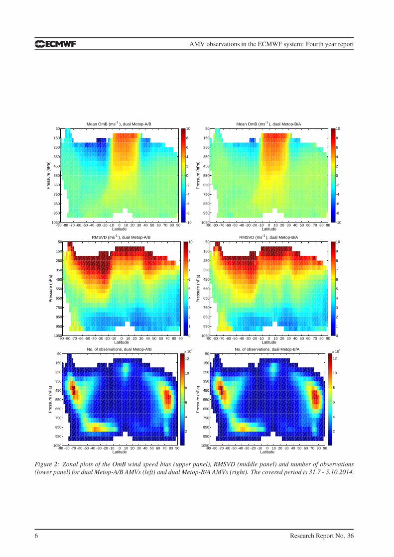
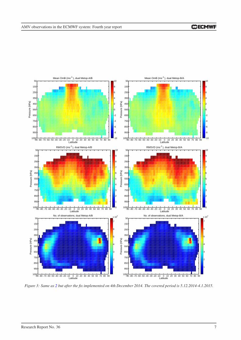
Figure 2 shows zonal plots of the OmB wind speed bias, RMSVD and number of observations for 31.7-

5.10.2014. The left panels are for dual Metop-A/B AMVs and the right panels for dual Metop-B/A AMVs.

In general, at high latitudes the bias and RMSVD statistics are very similar to the single Metop AMVs (note

different scale for bias compared to Fig. 1). The dual-Metop AMVs have large positive bias over the tropics,

especially above 700 hPa. The bias is larger in magnitude and more wide spread compared to what is seen for

AMVs from geostationary satellites. However, outside the tropics the data indicates promising potential for

further investigations.

The zonal plots reveal quite significant differences in the OmB speed bias and RMSVD for dual Metop-A/B

and Metop-B/A AMVs. EUMETSAT has investigated the issue and the explanation is that the planned small

drift of the satellites on the orbit was not taken into account in the AMV derivation. Initially the time difference

between Metop-A and Metop-B has been 45 min / 55 min but is now closer to 49 min / 51 min. A fix to

correct this issue and to prevent it happening again has been introduced to the operational processing on 4th



-90 -80 -70 -60 -50 -40 -30 -20 -10 0 10 20 30 40 50 60 70 80 901050

950

850

750

650

550

450

350

250

150

Latitude

Pre

ssur

e (h

Pa)

Mean OmB (ms-1 ), Metop-B AVHRR

-2

-1.5

-1

-0.5

0

0.5

1

1.5

2

-90 -80 -70 -60 -50 -40 -30 -20 -10 0 10 20 30 40 50 60 70 80 901050

950

850

750

650

550

450

350

250

150

LatitudeP

ress

ure

(hP

a)

Mean OmB (ms-1 ), Metop-B AVHRR

-2

-1.5

-1

-0.5

0

0.5

1

1.5

2

-90 -80 -70 -60 -50 -40 -30 -20 -10 0 10 20 30 40 50 60 70 80 901050

950

850

750

650

550

450

350

250

150

Latitude

Pre

ssur

e (h

Pa)

RMSVD (ms-1 ), Metop-B AVHRR

0

1

2

3

4

5

6

7

8

9

10

-90 -80 -70 -60 -50 -40 -30 -20 -10 0 10 20 30 40 50 60 70 80 901050

950

850

750

650

550

450

350

250

150

Latitude

Pre

ssur

e (h

Pa)

RMSVD (ms-1 ), Metop-B AVHRR

0

1

2

3

4

5

6

7

8

9

10

-90 -80 -70 -60 -50 -40 -30 -20 -10 0 10 20 30 40 50 60 70 80 901050

950

850

750

650

550

450

350

250

150

Latitude

Pre

ssur

e (h

Pa)

No. of observations, Metop-B AVHRR

0.5

1

1.5

2

2.5

x 104

-90 -80 -70 -60 -50 -40 -30 -20 -10 0 10 20 30 40 50 60 70 80 901050

950

850

750

650

550

450

350

250

150

Latitude

Pre

ssur

e (h

Pa)

No. of observations, Metop-B AVHRR

0.5

1

1.5

2

2.5

3

3.5

4

4.5

x 104

Figure 1: Zonal plots of the OmB wind speed bias (upper panels), RMSVD (middle panels) and number of observations

(lower panel) for Metop-B AMVs. The covered periods are two months before, 27.3. - 26.5.2014 (left), and two months

after, 28.5-27.7.2014 (right), the changes were implemented.

December 2014. Figure 3 shows the same as Fig. 2 for a one month period after the change was implemented

(5.12.2014-4.1.2015). The statistics for Metop-A/B and Metop-B/A are very similar to each other.



-90 -80 -70 -60 -50 -40 -30 -20 -10 0 10 20 30 40 50 60 70 80 901050

950

850

750

650

550

450

350

250

150

50

Latitude

Pre

ssur

e (h

Pa)

Mean OmB (ms-1 ), dual Metop-A/B

-10

-8

-6

-4

-2

0

2

4

6

8

10

-90 -80 -70 -60 -50 -40 -30 -20 -10 0 10 20 30 40 50 60 70 80 901050

950

850

750

650

550

450

350

250

150

50

Latitude

Pre

ssur

e (h

Pa)

Mean OmB (ms-1 ), dual Metop-B/A

-10

-8

-6

-4

-2

0

2

4

6

8

10

-90 -80 -70 -60 -50 -40 -30 -20 -10 0 10 20 30 40 50 60 70 80 901050

950

850

750

650

550

450

350

250

150

50

Latitude

Pre

ssur

e (h

Pa)

RMSVD (ms-1 ), dual Metop-A/B

0

1

2

3

4

5

6

7

8

9

10

-90 -80 -70 -60 -50 -40 -30 -20 -10 0 10 20 30 40 50 60 70 80 901050

950

850

750

650

550

450

350

250

150

50

Latitude

Pre

ssur

e (h

Pa)

RMSVD (ms-1 ), dual Metop-B/A

0

1

2

3

4

5

6

7

8

9

10

-90 -80 -70 -60 -50 -40 -30 -20 -10 0 10 20 30 40 50 60 70 80 901050

950

850

750

650

550

450

350

250

150

50

Latitude

Pre

ssur

e (h

Pa)

No. of observations, dual Metop-A/B

2

4

6

8

10

12

x 104

-90 -80 -70 -60 -50 -40 -30 -20 -10 0 10 20 30 40 50 60 70 80 901050

950

850

750

650

550

450

350

250

150

50

Latitude

Pre

ssur

e (h

Pa)

No. of observations, dual Metop-B/A

2

4

6

8

10

12

x 104

Figure 2: Zonal plots of the OmB wind speed bias (upper panel), RMSVD (middle panel) and number of observations

(lower panel) for dual Metop-A/B AMVs (left) and dual Metop-B/A AMVs (right). The covered period is 31.7 - 5.10.2014.



-90 -80 -70 -60 -50 -40 -30 -20 -10 0 10 20 30 40 50 60 70 80 901050

950

850

750

650

550

450

350

250

150

50

Latitude

Pre

ssur

e (h

Pa)

Mean OmB (ms-1 ), dual Metop-A/B

-10

-8

-6

-4

-2

0

2

4

6

8

10

-90 -80 -70 -60 -50 -40 -30 -20 -10 0 10 20 30 40 50 60 70 80 901050

950

850

750

650

550

450

350

250

150

50

Latitude

Pre

ssur

e (h

Pa)

Mean OmB (ms-1 ), dual Metop-B/A

-10

-8

-6

-4

-2

0

2

4

6

8

10

-90 -80 -70 -60 -50 -40 -30 -20 -10 0 10 20 30 40 50 60 70 80 901050

950

850

750

650

550

450

350

250

150

50

Latitude

Pre

ssur

e (h

Pa)

RMSVD (ms-1 ), dual Metop-A/B

0

1

2

3

4

5

6

7

8

9

10

-90 -80 -70 -60 -50 -40 -30 -20 -10 0 10 20 30 40 50 60 70 80 901050

950

850

750

650

550

450

350

250

150

50

Latitude

Pre

ssur

e (h

Pa)

RMSVD (ms-1 ), dual Metop-B/A

0

1

2

3

4

5

6

7

8

9

10

-90 -80 -70 -60 -50 -40 -30 -20 -10 0 10 20 30 40 50 60 70 80 901050

950

850

750

650

550

450

350

250

150

50

Latitude

Pre

ssur

e (h

Pa)

No. of observations, dual Metop-A/B

1

2

3

4

5

6

7

x 104

-90 -80 -70 -60 -50 -40 -30 -20 -10 0 10 20 30 40 50 60 70 80 901050

950

850

750

650

550

450

350

250

150

50

Latitude

Pre

ssur

e (h

Pa)

No. of observations, dual Metop-B/A

1

2

3

4

5

6

7

x 104

Figure 3: Same as 2 but after the fix implemented on 4th December 2014. The covered period is 5.12.2014-4.1.2015.



3 AMVs over the Indian Ocean

Currently, Meteosat-7 is the prime satellite to provide AMV coverage over the Indian Ocean. Securing the

AMV coverage over that area after Meteosat-7 has reached its lifetime is considered to be very important. A

comprehensive comparison of the options with impact assessment is presented in Cotton (2013). EUMETSAT

has expressed also a strong interest in results investigating the available options in the ECMWF system to

support the decision making process.

AMVs covering the Indian Ocean region are available from Meteosat-7 (57.5◦E; EUMETSAT, Carranza et al.

(2014)), FY-2D/E (86.5◦E/105◦E; CMA, Zhang et al. (2014)), Kalpana-1 and INSAT-3D (74◦E and 82◦E; IMD,

Deb (2012)). In the future EUMETSAT is planning to provide coverage for the Indian Ocean by moving

Meteosat-8 over the region. AMVs and radiance data from Meteosat-8 positioned over the Indian Ocean is

expected to provide better quality data than Meteosat-7.

AMVs from Meteosat-7 are operationally used in the ECMWF system. In addition, the quality of AMVs

from FY-2D and FY-2E are operationally passively monitored. The latest addition to the AMVs providing

coverage over the Indian Ocean are the INSAT-3D AMVs. Currently INSAT-3D AMVs are processed for

offline monitoring at ECMWF but they are planned to be added to the operational monitoring in the next update

to the IFS cycle.

In the following, first results from monitoring the quality of INSAT-3D AMVs and a comparison of the char-

acteristics to Meteosat-7 and FY-2E AMVs are presented. The impact of Meteosat-7 and FY-2E has been

investigated and these results will be discussed. Impact assessment of the INSAT-3D AMVs has not been com-

pleted yet as the data was not available at the time when the impact studies with Meteosat-7 and FY-2E were

performed.

3.1 Monitoring of Indian Ocean AMVs

AMVs from INSAT-3D have recently become available via the GTS. Processing of the data started at ECMWF

2nd October 2014. Here, first results of the passive monitoring are presented and the quality of INSAT-3D

AMVs is compared with the quality of Meteosat-7 and FY-2E AMVs.

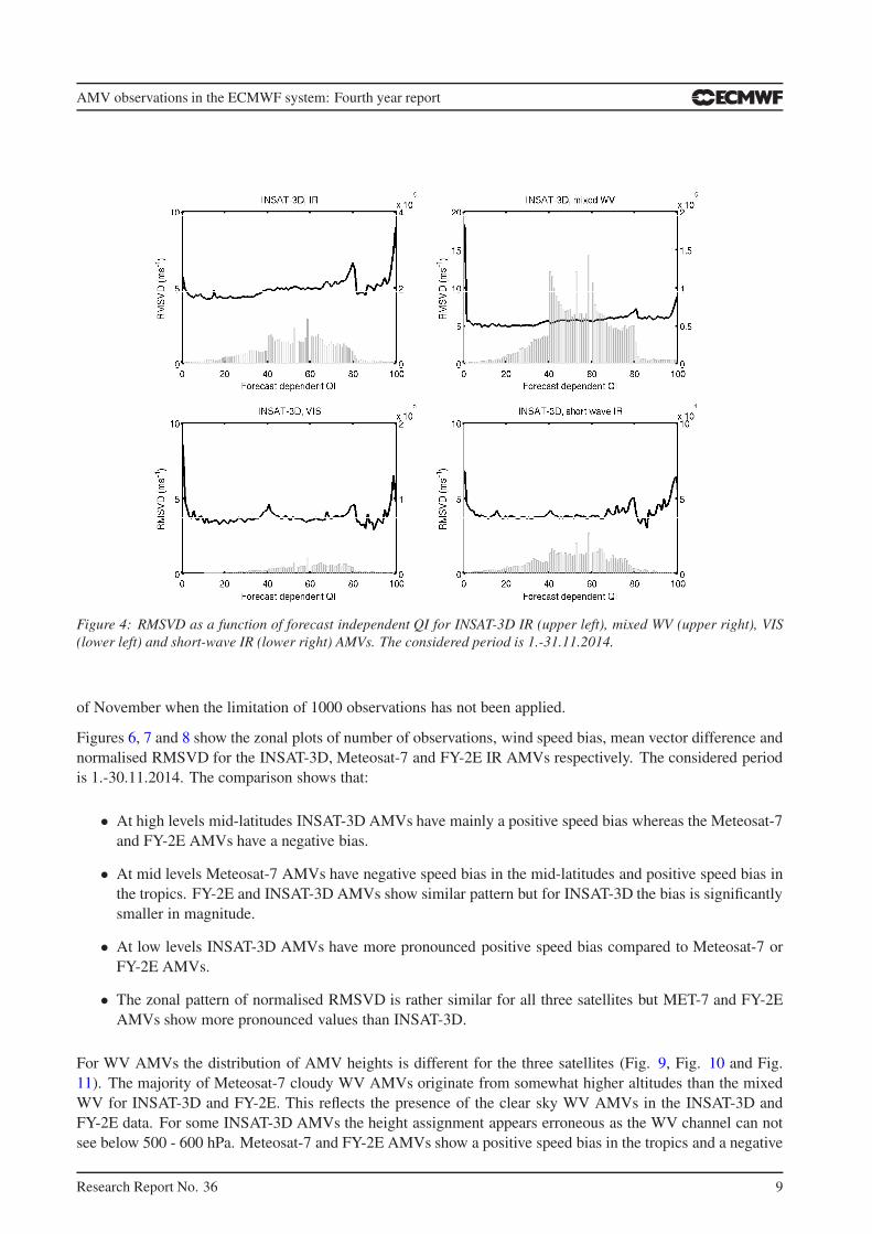
INSAT-3D AMVs are available from IR (10.8 m), VIS (0.65 m), Short-wave IR (3.8 m) and WV (6.9 m)

channels. There is no separation between cloudy and clear sky WV AMVs. The quality information provided

for the AMVs is the forecast independent QI. Figure 4 shows the RMSVD for different QI values. There are

very few observations with QI > 80. In addition, there is no clear dependence between RMSVD and QI. Thus,

in the following monitoring statistics no QI criterion is applied to the INSAT-3D data.

Meteosat-7 AMVs are available 1.5-hourly from IR (11.3 m), VIS (0.7 m) and WV (6.3 m) channels. Here,

only cloudy WV AMVs are considered. FY-2E AMVs are available 6-hourly from IR (10.8 m) and WV (6.8

m) channels. FY-2E WV AMVs are also a mix of cloudy and clear sky AMVs. For the Meteosat-7 and FY-2E

statistics the forecast independent QI > 80 criterion is applied. This is the standard NWP SAF monitoring QI

threshold. However, it is worth to note that for FY-2E the forecast independent and dependent QI are set to the

same value and in practise it is the forecast dependent QI.

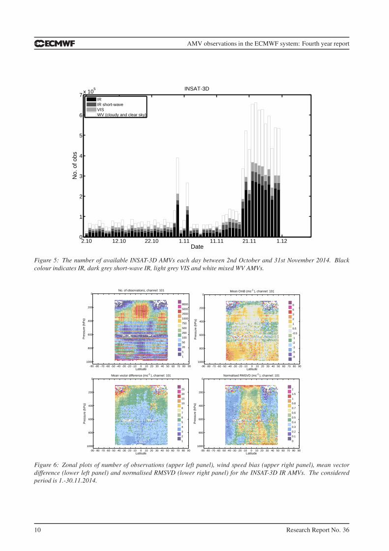
The number of available INSAT-3D AMVs is strongly fluctuating over time. Figure 5 shows the number of

available observations each day between 2nd October and 30th November 2014. Until 20th November 2014

most of the time at most 1000 observations per time and channel have been distributed. Frequently, the number

of winds is precisely 1000 per time-slot, suggesting a technical limitation. After 20th November the number of

available observations has increased significantly. However, there are dates at the end of October and beginning



Figure 4: RMSVD as a function of forecast independent QI for INSAT-3D IR (upper left), mixed WV (upper right), VIS

(lower left) and short-wave IR (lower right) AMVs. The considered period is 1.-31.11.2014.

of November when the limitation of 1000 observations has not been applied.

Figures 6, 7 and 8 show the zonal plots of number of observations, wind speed bias, mean vector difference and

normalised RMSVD for the INSAT-3D, Meteosat-7 and FY-2E IR AMVs respectively. The considered period

is 1.-30.11.2014. The comparison shows that:

• At high levels mid-latitudes INSAT-3D AMVs have mainly a positive speed bias whereas the Meteosat-7

and FY-2E AMVs have a negative bias.

• At mid levels Meteosat-7 AMVs have negative speed bias in the mid-latitudes and positive speed bias in

the tropics. FY-2E and INSAT-3D AMVs show similar pattern but for INSAT-3D the bias is significantly

smaller in magnitude.

• At low levels INSAT-3D AMVs have more pronounced positive speed bias compared to Meteosat-7 or

FY-2E AMVs.

• The zonal pattern of normalised RMSVD is rather similar for all three satellites but MET-7 and FY-2E

AMVs show more pronounced values than INSAT-3D.

For WV AMVs the distribution of AMV heights is different for the three satellites (Fig. 9, Fig. 10 and Fig.

11). The majority of Meteosat-7 cloudy WV AMVs originate from somewhat higher altitudes than the mixed

WV for INSAT-3D and FY-2E. This reflects the presence of the clear sky WV AMVs in the INSAT-3D and

FY-2E data. For some INSAT-3D AMVs the height assignment appears erroneous as the WV channel can not

see below 500 - 600 hPa. Meteosat-7 and FY-2E AMVs show a positive speed bias in the tropics and a negative



2.10 12.10 22.10 1.11 11.11 21.11 1.120

1

2

3

4

5

6

7x 10

5

Date

No.

of o

bs

INSAT-3D

IRIR short-waveVISWV (cloudy and clear sky)

Figure 5: The number of available INSAT-3D AMVs each day between 2nd October and 31st November 2014. Black

colour indicates IR, dark grey short-wave IR, light grey VIS and white mixed WV AMVs.

-90 -80 -70 -60 -50 -40 -30 -20 -10 0 10 20 30 40 50 60 70 80 90

1000

800

600

400

200

0

8000

5000

2000

1000

750

500

200

100

50

20

5

1

Latitude

Pre

ssur

e (h

Pa)

No. of observations, channel: 101

-90 -80 -70 -60 -50 -40 -30 -20 -10 0 10 20 30 40 50 60 70 80 90

1000

800

600

400

200

0

Latitude

Pre

ssur

e (h

Pa)

Mean OmB (ms-1 ), channel: 101

8

5

3

2

1

0.5

-0.5

-1

-2

-3

-5

-8

-90 -80 -70 -60 -50 -40 -30 -20 -10 0 10 20 30 40 50 60 70 80 90

1000

800

600

400

200

0

Latitude

Pre

ssur

e (h

Pa)

Mean vector difference (ms-1 ), channel: 101

25

20

15

10

8

7

6

5

4

3

2

1

-90 -80 -70 -60 -50 -40 -30 -20 -10 0 10 20 30 40 50 60 70 80 90

1000

800

600

400

200

0

Latitude

Pre

ssur

e (h

Pa)

Normalised RMSVD (ms-1 ), channel: 101

2

1.5

1

0.8

0.7

0.6

0.5

0.4

0.3

0.2

0.1

0

Figure 6: Zonal plots of number of observations (upper left panel), wind speed bias (upper right panel), mean vector

difference (lower left panel) and normalised RMSVD (lower right panel) for the INSAT-3D IR AMVs. The considered

period is 1.-30.11.2014.



-90 -80 -70 -60 -50 -40 -30 -20 -10 0 10 20 30 40 50 60 70 80 90

1000

800

600

400

200

0

8000

5000

2000

1000

750

500

200

100

50

20

5

1

Latitude

Pre

ssur

e (h

Pa)


-90 -80 -70 -60 -50 -40 -30 -20 -10 0 10 20 30 40 50 60 70 80 90

1000

800

600

400

200

0

Latitude

Pre

ssur

e (h

Pa)


8

5

3

2

1

0.5

-0.5

-1

-2

-3

-5

-8

-90 -80 -70 -60 -50 -40 -30 -20 -10 0 10 20 30 40 50 60 70 80 90

1000

800

600

400

200

0

Latitude

Pre

ssur

e (h

Pa)


25

20

15

10

8

7

6

5

4

3

2

1

-90 -80 -70 -60 -50 -40 -30 -20 -10 0 10 20 30 40 50 60 70 80 90

1000

800

600

400

200

0

Latitude

Pre

ssur

e (h

Pa)


2

1.5

1

0.8

0.7

0.6

0.5

0.4

0.3

0.2

0.1

0

Figure 7: Same as 6 but for Meteosat-7 IR AMVs.

-90 -80 -70 -60 -50 -40 -30 -20 -10 0 10 20 30 40 50 60 70 80 90

1000

800

600

400

200

0

8000

5000

2000

1000

750

500

200

100

50

20

5

1

Latitude

Pre

ssur

e (h

Pa)


-90 -80 -70 -60 -50 -40 -30 -20 -10 0 10 20 30 40 50 60 70 80 90

1000

800

600

400

200

0

Latitude

Pre

ssur

e (h

Pa)


8

5

3

2

1

0.5

-0.5

-1

-2

-3

-5

-8

-90 -80 -70 -60 -50 -40 -30 -20 -10 0 10 20 30 40 50 60 70 80 90

1000

800

600

400

200

0

Latitude

Pre

ssur

e (h

Pa)


25

20

15

10

8

7

6

5

4

3

2

1

-90 -80 -70 -60 -50 -40 -30 -20 -10 0 10 20 30 40 50 60 70 80 90

1000

800

600

400

200

0

Latitude

Pre

ssur

e (h

Pa)


2

1.5

1

0.8

0.7

0.6

0.5

0.4

0.3

0.2

0.1

0

Figure 8: Same as 6 but for FY-2E IR AMVs.

bias in the mid-latitudes. The magnitude of the bias is more pronounced for the Meteosat-7 AMVs. INSAT-3D

AMVs do not have this kind of pattern. In general there are more regions with positive speed bias than with

negative for the INSAT-3D AMVs. Again, the RMSVD is rather similar for all three satellites.



-90 -80 -70 -60 -50 -40 -30 -20 -10 0 10 20 30 40 50 60 70 80 90

1000

800

600

400

200

0

8000

5000

2000

1000

750

500

200

100

50

20

5

1

Latitude

Pre

ssur

e (h

Pa)


-90 -80 -70 -60 -50 -40 -30 -20 -10 0 10 20 30 40 50 60 70 80 90

1000

800

600

400

200

0

Latitude

Pre

ssur

e (h

Pa)


8

5

3

2

1

0.5

-0.5

-1

-2

-3

-5

-8

-90 -80 -70 -60 -50 -40 -30 -20 -10 0 10 20 30 40 50 60 70 80 90

1000

800

600

400

200

0

Latitude

Pre

ssur

e (h

Pa)


25

20

15

10

8

7

6

5

4

3

2

1

-90 -80 -70 -60 -50 -40 -30 -20 -10 0 10 20 30 40 50 60 70 80 90

1000

800

600

400

200

0

Latitude

Pre

ssur

e (h

Pa)


2

1.5

1

0.8

0.7

0.6

0.5

0.4

0.3

0.2

0.1

0

Figure 9: Same as 6 but for INSAT-3D mixed WV AMVs.

-90 -80 -70 -60 -50 -40 -30 -20 -10 0 10 20 30 40 50 60 70 80 90

1000

800

600

400

200

0

8000

5000

2000

1000

750

500

200

100

50

20

5

1

Latitude

Pre

ssur

e (h

Pa)


-90 -80 -70 -60 -50 -40 -30 -20 -10 0 10 20 30 40 50 60 70 80 90

1000

800

600

400

200

0

Latitude

Pre

ssur

e (h

Pa)


8

5

3

2

1

0.5

-0.5

-1

-2

-3

-5

-8

-90 -80 -70 -60 -50 -40 -30 -20 -10 0 10 20 30 40 50 60 70 80 90

1000

800

600

400

200

0

Latitude

Pre

ssur

e (h

Pa)


25

20

15

10

8

7

6

5

4

3

2

1

-90 -80 -70 -60 -50 -40 -30 -20 -10 0 10 20 30 40 50 60 70 80 90

1000

800

600

400

200

0

Latitude

Pre

ssur

e (h

Pa)


2

1.5

1

0.8

0.7

0.6

0.5

0.4

0.3

0.2

0.1

0

Figure 10: Same as 6 but for Meteosat-7 cloudy WV AMVs.

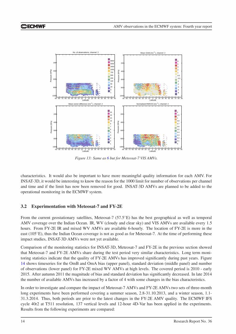
For the VIS AMVs the monitoring statistics are quite similar for INSAT-3D and Meteosat-7 satellites (Fig. 12

and Fig. 13). INSAT-3D AMVs are available below 500 hPa, Meteosat-7 below 700 hPa and in general there

are more Meteosat-7 AMVs available than INSAT-3D AMVs. For FY-2E VIS AMVs are not produced.



-90 -80 -70 -60 -50 -40 -30 -20 -10 0 10 20 30 40 50 60 70 80 90

1000

800

600

400

200

0

8000

5000

2000

1000

750

500

200

100

50

20

5

1

Latitude

Pre

ssur

e (h

Pa)


-90 -80 -70 -60 -50 -40 -30 -20 -10 0 10 20 30 40 50 60 70 80 90

1000

800

600

400

200

0

Latitude

Pre

ssur

e (h

Pa)


8

5

3

2

1

0.5

-0.5

-1

-2

-3

-5

-8

-90 -80 -70 -60 -50 -40 -30 -20 -10 0 10 20 30 40 50 60 70 80 90

1000

800

600

400

200

0

Latitude

Pre

ssur

e (h

Pa)


25

20

15

10

8

7

6

5

4

3

2

1

-90 -80 -70 -60 -50 -40 -30 -20 -10 0 10 20 30 40 50 60 70 80 90

1000

800

600

400

200

0

Latitude

Pre

ssur

e (h

Pa)


2

1.5

1

0.8

0.7

0.6

0.5

0.4

0.3

0.2

0.1

0

Figure 11: Same as 6 but for FY-2E mixed WV AMVs.

-90 -80 -70 -60 -50 -40 -30 -20 -10 0 10 20 30 40 50 60 70 80 90

1000

800

600

400

200

0

8000

5000

2000

1000

750

500

200

100

50

20

5

1

Latitude

Pre

ssur

e (h

Pa)


-90 -80 -70 -60 -50 -40 -30 -20 -10 0 10 20 30 40 50 60 70 80 90

1000

800

600

400

200

0

Latitude

Pre

ssur

e (h

Pa)


8

5

3

2

1

0.5

-0.5

-1

-2

-3

-5

-8

-90 -80 -70 -60 -50 -40 -30 -20 -10 0 10 20 30 40 50 60 70 80 90

1000

800

600

400

200

0

Latitude

Pre

ssur

e (h

Pa)


25

20

15

10

8

7

6

5

4

3

2

1

-90 -80 -70 -60 -50 -40 -30 -20 -10 0 10 20 30 40 50 60 70 80 90

1000

800

600

400

200

0

Latitude

Pre

ssur

e (h

Pa)


2

1.5

1

0.8

0.7

0.6

0.5

0.4

0.3

0.2

0.1

0

Figure 12: Same as 6 but for INSAT-3D VIS AMVs.

First conclusions from the monitoring indicate that the INSAT-3D and FY-2E AMVs show promising data

quality comparable to Meteosat-7, and there is potential for further investigations. From the NWP point of

view, it would be beneficial to separate cloudy and clear sky WV AMVs as they tend to show very different



-90 -80 -70 -60 -50 -40 -30 -20 -10 0 10 20 30 40 50 60 70 80 90

1000

800

600

400

200

0

8000

5000

2000

1000

750

500

200

100

50

20

5

1

Latitude

Pre

ssur

e (h

Pa)


-90 -80 -70 -60 -50 -40 -30 -20 -10 0 10 20 30 40 50 60 70 80 90

1000

800

600

400

200

0

Latitude

Pre

ssur

e (h

Pa)


8

5

3

2

1

0.5

-0.5

-1

-2

-3

-5

-8

-90 -80 -70 -60 -50 -40 -30 -20 -10 0 10 20 30 40 50 60 70 80 90

1000

800

600

400

200

0

Latitude

Pre

ssur

e (h

Pa)


25

20

15

10

8

7

6

5

4

3

2

1

-90 -80 -70 -60 -50 -40 -30 -20 -10 0 10 20 30 40 50 60 70 80 90

1000

800

600

400

200

0

Latitude

Pre

ssur

e (h

Pa)


2

1.5

1

0.8

0.7

0.6

0.5

0.4

0.3

0.2

0.1

0

Figure 13: Same as 6 but for Meteosat-7 VIS AMVs.

characteristics. It would also be important to have more meaningful quality information for each AMV. For

INSAT-3D, it would be interesting to know the reason for the 1000 limit for number of observations per channel

and time and if the limit has now been removed for good. INSAT-3D AMVs are planned to be added to the

operational monitoring in the ECMWF system.

3.2 Experimentation with Meteosat-7 and FY-2E

From the current geostationary satellites, Meteosat-7 (57.5◦E) has the best geographical as well as temporal

AMV coverage over the Indian Ocean. IR, WV (cloudy and clear sky) and VIS AMVs are available every 1.5

hours. From FY-2E IR and mixed WV AMVs are available 6-hourly. The location of FY-2E is more in the

east (105◦E), thus the Indian Ocean coverage is not as good as for Meteosat-7. At the time of performing these

impact studies, INSAT-3D AMVs were not yet available.

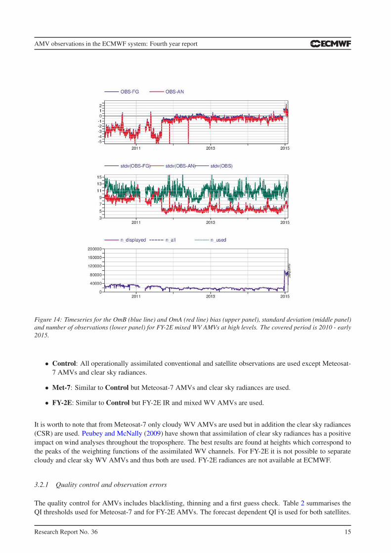
Comparison of the monitoring statistics for INSAT-3D, Meteosat-7 and FY-2E in the previous section showed

that Meteosat-7 and FY-2E AMVs share during the test period very similar characteristics. Long term moni-

toring statistics indicate that the quality of FY-2E AMVs has improved significantly during past years. Figure

14 shows timeseries for the OmB and OmA bias (upper panel), standard deviation (middle panel) and number

of observations (lower panel) for FY-2E mixed WV AMVs at high levels. The covered period is 2010 - early

2015. After autumn 2011 the magnitude of bias and standard deviation has significantly decreased. In late 2014

the number of available AMVs has increased by a factor of 4 with some changes in the bias characteristics.

In order to investigate and compare the impact of Meteosat-7 AMVs and FY-2E AMVs two sets of three-month

long experiments have been performed covering a summer season, 2.8-31.10.2013, and a winter season, 1.1-

31.3.2014. Thus, both periods are prior to the latest changes in the FY-2E AMV quality. The ECMWF IFS

cycle 40r2 at T511 resolution, 137 vertical levels and 12-hour 4D-Var has been applied in the experiments.

Results from the following experiments are compared:



Figure 14: Timeseries for the OmB (blue line) and OmA (red line) bias (upper panel), standard deviation (middle panel)

and number of observations (lower panel) for FY-2E mixed WV AMVs at high levels. The covered period is 2010 - early

2015.

• Control: All operationally assimilated conventional and satellite observations are used except Meteosat-

7 AMVs and clear sky radiances.

• Met-7: Similar to Control but Meteosat-7 AMVs and clear sky radiances are used.

• FY-2E: Similar to Control but FY-2E IR and mixed WV AMVs are used.

It is worth to note that from Meteosat-7 only cloudy WV AMVs are used but in addition the clear sky radiances

(CSR) are used. Peubey and McNally (2009) have shown that assimilation of clear sky radiances has a positive

impact on wind analyses throughout the troposphere. The best results are found at heights which correspond to

the peaks of the weighting functions of the assimilated WV channels. For FY-2E it is not possible to separate

cloudy and clear sky WV AMVs and thus both are used. FY-2E radiances are not available at ECMWF.

3.2.1 Quality control and observation errors

The quality control for AMVs includes blacklisting, thinning and a first guess check. Table 2 summarises the

QI thresholds used for Meteosat-7 and for FY-2E AMVs. The forecast dependent QI is used for both satellites.



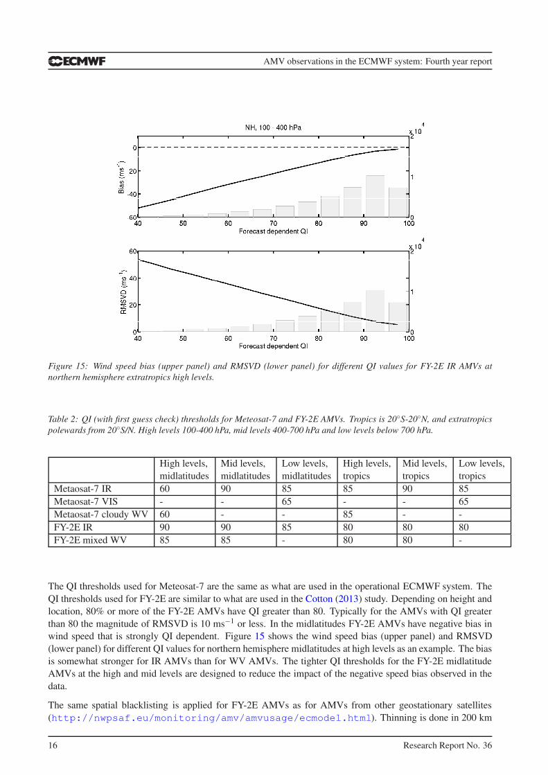
Figure 15: Wind speed bias (upper panel) and RMSVD (lower panel) for different QI values for FY-2E IR AMVs at

northern hemisphere extratropics high levels.

Table 2: QI (with first guess check) thresholds for Meteosat-7 and FY-2E AMVs. Tropics is 20◦S-20◦N, and extratropics

polewards from 20◦S/N. High levels 100-400 hPa, mid levels 400-700 hPa and low levels below 700 hPa.

High levels, Mid levels, Low levels, High levels, Mid levels, Low levels,

midlatitudes midlatitudes midlatitudes tropics tropics tropics

Metaosat-7 IR 60 90 85 85 90 85

Metaosat-7 VIS - - 65 - - 65

Metaosat-7 cloudy WV 60 - - 85 - -

FY-2E IR 90 90 85 80 80 80

FY-2E mixed WV 85 85 - 80 80 -

The QI thresholds used for Meteosat-7 are the same as what are used in the operational ECMWF system. The

QI thresholds used for FY-2E are similar to what are used in the Cotton (2013) study. Depending on height and

location, 80% or more of the FY-2E AMVs have QI greater than 80. Typically for the AMVs with QI greater

than 80 the magnitude of RMSVD is 10 ms−1 or less. In the midlatitudes FY-2E AMVs have negative bias in

wind speed that is strongly QI dependent. Figure 15 shows the wind speed bias (upper panel) and RMSVD

(lower panel) for different QI values for northern hemisphere midlatitudes at high levels as an example. The bias

is somewhat stronger for IR AMVs than for WV AMVs. The tighter QI thresholds for the FY-2E midlatitude

AMVs at the high and mid levels are designed to reduce the impact of the negative speed bias observed in the

data.

The same spatial blacklisting is applied for FY-2E AMVs as for AMVs from other geostationary satellites

(http://nwpsaf.eu/monitoring/amv/amvusage/ecmodel.html). Thinning is done in 200 km


http://nwpsaf.eu/monitoring/amv/amvusage/ecmodel.html


0 100 200 300

950

850

750

650

550

450

350

250

150

50

Height error (hPa)

Pre

ssur

e (h

Pa)

WV

MET-7FY-2E

0 100 200 300

950

850

750

650

550

450

350

250

150

50

Height error (hPa)

Pre

ssur

e (h

Pa)

IR

MET-7FY-2E

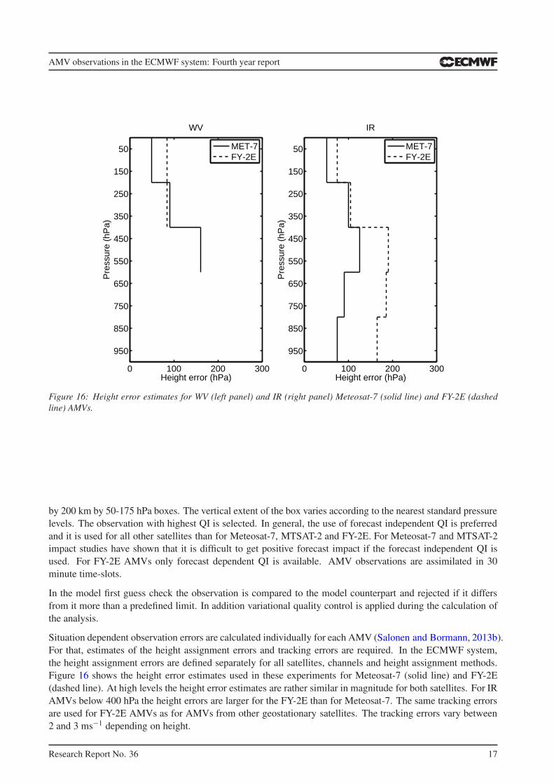
Figure 16: Height error estimates for WV (left panel) and IR (right panel) Meteosat-7 (solid line) and FY-2E (dashed

line) AMVs.

by 200 km by 50-175 hPa boxes. The vertical extent of the box varies according to the nearest standard pressure

levels. The observation with highest QI is selected. In general, the use of forecast independent QI is preferred

and it is used for all other satellites than for Meteosat-7, MTSAT-2 and FY-2E. For Meteosat-7 and MTSAT-2

impact studies have shown that it is difficult to get positive forecast impact if the forecast independent QI is

used. For FY-2E AMVs only forecast dependent QI is available. AMV observations are assimilated in 30

minute time-slots.

In the model first guess check the observation is compared to the model counterpart and rejected if it differs

from it more than a predefined limit. In addition variational quality control is applied during the calculation of

the analysis.

Situation dependent observation errors are calculated individually for each AMV (Salonen and Bormann, 2013b).

For that, estimates of the height assignment errors and tracking errors are required. In the ECMWF system,

the height assignment errors are defined separately for all satellites, channels and height assignment methods.

Figure 16 shows the height error estimates used in these experiments for Meteosat-7 (solid line) and FY-2E

(dashed line). At high levels the height error estimates are rather similar in magnitude for both satellites. For IR

AMVs below 400 hPa the height errors are larger for the FY-2E than for Meteosat-7. The same tracking errors

are used for FY-2E AMVs as for AMVs from other geostationary satellites. The tracking errors vary between

2 and 3 ms−1 depending on height.



99.7 99.8 99.9 100.0 100.1 100.2 100.3Analysis std. dev. [%, normalised]

1000

850

700

500

400

300

250

200

150

100

70

50

30

20

10

Pre

ssur

e [h

Pa]

99.7 99.8 99.9 100.0 100.1 100.2 100.3FG std. dev. [%, normalised]

a b

Instrument(s): AIREP AMprofiler EUprofiler JPprofiler PILOT TEMP − Uwind VwindArea(s): Europe Japan N.Amer N.Hemis S.Hemis Tropics

From 00Z 2−Aug−2013 to 12Z 31−Mar−2014

Mg5g9Mg5ga

Mg5slMg5sn

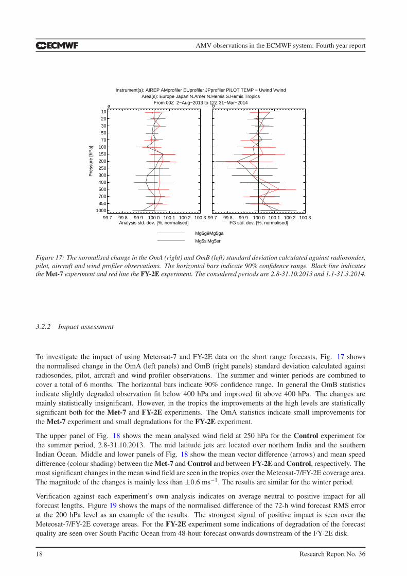
Figure 17: The normalised change in the OmA (right) and OmB (left) standard deviation calculated against radiosondes,

pilot, aircraft and wind profiler observations. The horizontal bars indicate 90% confidence range. Black line indicates

the Met-7 experiment and red line the FY-2E experiment. The considered periods are 2.8-31.10.2013 and 1.1-31.3.2014.

3.2.2 Impact assessment

To investigate the impact of using Meteosat-7 and FY-2E data on the short range forecasts, Fig. 17 shows

the normalised change in the OmA (left panels) and OmB (right panels) standard deviation calculated against

radiosondes, pilot, aircraft and wind profiler observations. The summer and winter periods are combined to

cover a total of 6 months. The horizontal bars indicate 90% confidence range. In general the OmB statistics

indicate slightly degraded observation fit below 400 hPa and improved fit above 400 hPa. The changes are

mainly statistically insignificant. However, in the tropics the improvements at the high levels are statistically

significant both for the Met-7 and FY-2E experiments. The OmA statistics indicate small improvements for

the Met-7 experiment and small degradations for the FY-2E experiment.

The upper panel of Fig. 18 shows the mean analysed wind field at 250 hPa for the Control experiment for

the summer period, 2.8-31.10.2013. The mid latitude jets are located over northern India and the southern

Indian Ocean. Middle and lower panels of Fig. 18 show the mean vector difference (arrows) and mean speed

difference (colour shading) between the Met-7 and Control and between FY-2E and Control, respectively. The

most significant changes in the mean wind field are seen in the tropics over the Meteosat-7/FY-2E coverage area.

The magnitude of the changes is mainly less than ±0.6 ms−1. The results are similar for the winter period.

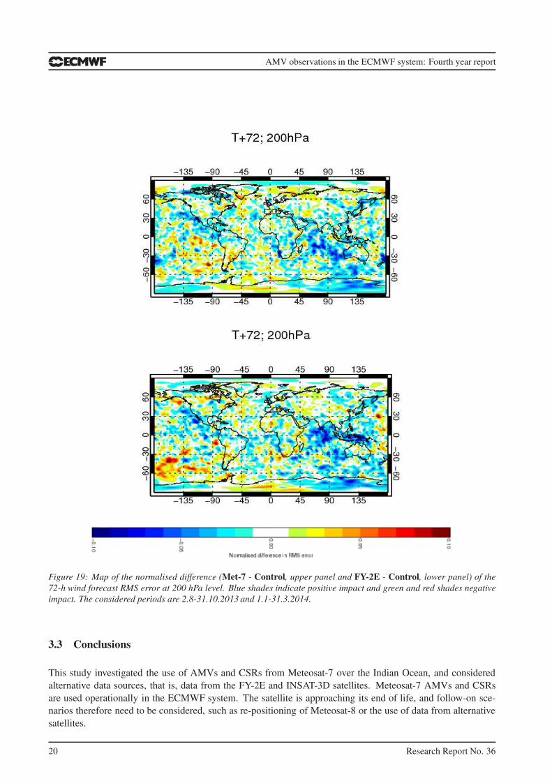
Verification against each experiment’s own analysis indicates on average neutral to positive impact for all

forecast lengths. Figure 19 shows the maps of the normalised difference of the 72-h wind forecast RMS error

at the 200 hPa level as an example of the results. The strongest signal of positive impact is seen over the

Meteosat-7/FY-2E coverage areas. For the FY-2E experiment some indications of degradation of the forecast

quality are seen over South Pacific Ocean from 48-hour forecast onwards downstream of the FY-2E disk.



0°N

30°S

60°S

30°N

60°N

0°N

30°S

60°S

30°N

60°N

0°E60°W120°W 60°E 120°E

0°E60°W120°W 60°E 120°E

LEV=250, 20130802 to 20131031Mean analysis of vector wind, Exp=g5ht

Friday 02 August 2013 00 UTC ecmf t+0 VT:Friday 02 August 2013 00 UTC 250 hPa U component of wind/V component of wind

0.2

0.60°N

30°S

60°S

30°N

60°N

0°N

30°S

60°S

30°N

60°N

0°E60°W120°W 60°E 120°E

0°E60°W120°W 60°E 120°E

LEV=250, 20130802 to 20131031Vector difference of mean wind analysis, Exps g5g9-g5ht

Friday 02 August 2013 00 UTC ecmf t+0 VT:Friday 02 August 2013 00 UTC 250 hPa U component of wind Friday 02 August 2013 00 UTC ecmf t+0 VT:Friday 02 August 2013 00 UTC 250 hPa U component of wind/V component of wind

-2 -1.8 -1.6 -1.4 -1.2 -1 -0.8 -0.6 -0.4 -0.2 0.2 0.4 0.6 0.8 1 1.2 1.4 1.6 1.8 2

0.2

0.20°N

30°S

60°S

30°N

60°N

0°N

30°S

60°S

30°N

60°N

0°E60°W120°W 60°E 120°E

0°E60°W120°W 60°E 120°E

LEV=250, 20130802 to 20131031Vector difference of mean wind analysis, Exps g5sl-g5ht

Friday 02 August 2013 00 UTC ecmf t+0 VT:Friday 02 August 2013 00 UTC 250 hPa U component of wind Friday 02 August 2013 00 UTC ecmf t+0 VT:Friday 02 August 2013 00 UTC 250 hPa U component of wind/V component of wind

-2 -1.8 -1.6 -1.4 -1.2 -1 -0.8 -0.6 -0.4 -0.2 0.2 0.4 0.6 0.8 1 1.2 1.4 1.6 1.8 2

Figure 18: The mean analysed wind field at 250 hPa for the Control experiment (upper panel). Difference in the mean

wind analysis at 250 hPa between the Control and Met-7 experiments (middle panel) and between the Control and

FY-2E experiments (lower panel). The considered period is 2.8-31.10.2013.



Figure 19: Map of the normalised difference (Met-7 - Control, upper panel and FY-2E - Control, lower panel) of the

72-h wind forecast RMS error at 200 hPa level. Blue shades indicate positive impact and green and red shades negative

impact. The considered periods are 2.8-31.10.2013 and 1.1-31.3.2014.

3.3 Conclusions

This study investigated the use of AMVs and CSRs from Meteosat-7 over the Indian Ocean, and considered

alternative data sources, that is, data from the FY-2E and INSAT-3D satellites. Meteosat-7 AMVs and CSRs

are used operationally in the ECMWF system. The satellite is approaching its end of life, and follow-on sce-

narios therefore need to be considered, such as re-positioning of Meteosat-8 or the use of data from alternative

satellites.



The CMA operated FY-2E and IMD operated INSAT-3D AMVs are also providing coverage over the Indian

Ocean. The FY-2E AMVs are available 6-hourly, compared to the 1 1/2 hourly availability of Meteosat-7

AMVs, whereas the INSAT-3D AMVs have varying time intervals. Long term monitoring of the FY-2E AMVs

indicate that there has been significant improvements in the data quality during the past years. The current

monitoring statistics for the FY-2E and INSAT-3D AMVs are generally in line with what is seen for other

geostationary satellites. However, there is no separation for the clear sky and cloudy WV AMVs and neither

of the satellites provide CSR or ASR (all sky radiance) observations. There are also some issues with the

provided QI information. For FY-2E AMVs only forecast dependent QI is available. For INSAT-3D AMVs the

provided QI is not currently very meaningful. AMVs from both satellites indicate good potential for further

investigations but the Metosat-7 observations still have advantages over INSAT-3D or FY-2E. It is also worth

noting here that AMVs and radiance data from Meteosat-8 positioned over the Indian Ocean is expected to

provide better quality data than Meteosat-7.

Our impact study shows positive forecast impact when Meteosat-7 AMVs and CSRs or FY-2E AMVs are

assimilated, with a slight advantage for the Meteosat-7 data. It is therefore clear that maintaining the Indian

Ocean coverage is important. An impact assessment of the INSAT-3D AMVs has not been done yet, but will

be considered in the near future.

4 Situation dependent observation errors with default values

The use of AMVs in the ECMWF system has been revised (Salonen and Bormann, 2013b). The aim of the

changes is to ensure effective and realistic use of AMVs in data assimilation in order to improve their impact

on model analyses and forecasts. The main amendment is the introduction of situation dependent observation

errors. This is done to ensure that the errors assigned in the data assimilation better account for height as-

signment errors of the observations. The use of situation dependent observation errors allowed also notable

simplifications to the AMV quality control. The modifications are included in the ECMWF IFS cycle 40r1

which became operational in November 2013.

One of the core activities at ECMWF is to produce reanalyses which aim to provide the best estimate of the

state of the atmosphere over several decades. This is achieved by using the same state-of-the-art NWP system

for the entire period and by using improved versions of the available observational datasets. Several satellite

agencies have recently made available reprocessed AMVs for reanalyses purposes.

In the operational ECMWF system the height and tracking error estimates are defined for all satellites, channels

and height assignment methods and they vary with height. The error estimates are updated every time when a

new satellite is introduced to the system or when AMV providers make changes in their processing. Estimating

the height and tracking errors for all historical AMVs would be an extensive effort. Thus, the impact of using

default error values for height assignment and tracking errors instead of the more tailored error estimates has

been investigated.

In the operational system default values of 80 hPa for the height error and 2.5 ms−1 for the tracking error are

used in case the tailored values do not exist. These values can be thought to be on average valid for AMVs but

obviously in some cases they are underestimating and in some cases overestimating the errors. To study the

impact of using the default values instead of tailored error estimates two two-month long experiments covering

a summer period 1.7-31.8.2013 have been performed. The ECMWF IFS cycle 40r1 at T511 resolution, 137

vertical levels and 12-hour 4D-Var has been applied in the experiments. The control experiment (Ctl) uses the

operationally used height and tracking errors for AMVs while the second experiment (Default) uses the default

height and tracking error values for all AMVs. In both experiments all operationally assimilated conventional

and satellite observations are used.



01e52e53e54e55e56e57e58e59e510e5

No. observations

2 3 4 5 6 71050

950

850

750

650

550

450

350

250

150

50

Mean obs error (ms-1 )

Pre

ssur

e (h

Pa)

CtlDefault

Figure 20: Average observation errors for Meteosat-10 AMVs at different heights. The solid line indicates the Ctl exper-

iment with the tailored height and tracking errors and the dashed line the Default experiment applying the default error

values. The grey bars show the number of observations for the Ctl experiment.

Generally, the resulting observation errors for wind components u and v are on average somewhat lower when

the default values are applied for the height assignment and tracking errors instead of the tailored error es-

timates. Figure 20 shows the average observation errors for Meteosat-10 AMVs at different heights as an

example. The solid line indicates the Ctl experiment with the tailored height and tracking errors and the dashed

line the Default experiment applying the default error values. The largest differences between the average ob-

servation errors are seen at mid levels, where the default value of 80 hPa is an underestimate of the uncertainty

in height assignment. However, most of the AMVs originate from high and low levels where the differences in

the average observation errors are not very drastic.

The model first guess check compares observations to their model counterparts. If the observation differs from

the model counterpart more than a predefined limit, it will be rejected. The first guess check rejections are

dependent on the magnitude of the observation and background errors. Due to somewhat higher observation

errors in the Ctl experiment more AMVs pass the first guess check and are used in the model analyses. Figure

21 shows the change in the number of observations (left) and the actual number of observations (right). In the

Default experiment 90% - close to 100% observations are used compared to the Ctl experiment. The difference

is smallest over the northern hemisphere.

To investigate the impact of using the default error values on the short term forecasts, figure 22 shows the

normalised change in the OmA (left panel) and OmB (right panel) standard deviation calculated against ra-



70 75 80 85 90 95 100 105number [%, normalised]

1000

850

700

500

400

300

250

200

150

100P

ress

ure

[hP

a]

0 1•106 2•106 3•106 4•106

number

a b

Instrument(s): SATOB−Uwind SATOB−Vwind Area(s): Antarctic Arctic N.Midlat S.Midlat TropicsFrom 00Z 1−Jul−2013 to 12Z 31−Aug−2013

fzddfyn7

Figure 21: The change in the number of observations compared to Ctl experiment (left) and the actual number of obser-

vations (right). Black line indicates the Default experiment and red line the Ctl experiment.

99.6 99.8 100.0 100.2 100.4 100.6Analysis std. dev. [%, normalised]

1000

850

700

500

400

300

250

200

150

100

70

50

30

20

10

Pre

ssur

e [h

Pa]

99.6 99.8 100.0 100.2 100.4 100.6FG std. dev. [%, normalised]

a b

Instrument(s): AIREP AMprofiler EUprofiler JPprofiler PILOT TEMP − Uwind VwindArea(s): Europe Japan N.Amer N.Hemis S.Hemis Tropics

From 00Z 1−Jul−2013 to 12Z 31−Aug−2013

fzdd

Figure 22: The normalised change in the OmA (left panel) and OmB (right panel) standard deviation calculated against

radiosondes, pilot, aircraft and wind profiler observations. The horizontal bars indicate 90% confidence range.

diosondes, pilot, aircraft and wind profiler observations. The horizontal bars indicate the 90% confidence

range. The changes both in the OmB and OmA statistics are mainly statistically insignificant. However, be-

tween 400 and 200 hPa the OmB statistics show negative impact and for the southern hemisphere (not shown

separately) the impact is also statistically significant. This indicates that the other wind observations fit slightly

worse the model first guess when the default values for the height assignment and tracking errors are used.

Figure 23 shows the zonal plots of the normalised difference (Default - Ctl) of the RMS wind error for 24-hour

and 48-hour forecast lengths. The impact of using the default values for the height assignment and tracking

errors is neutral compared to using the tailored values.

Based on the results it can be concluded that using the default height assignment and tracking error values



Figure 23: Zonal plots of the normalised difference (Default - Ctl) of the RMS wind error for 24-hour and 48-hour

forecasts. Blue shades indicate positive impact from using the default error values and red shades negative impact. The

cross-hatching indicates statistical significance at 95%. The considered period is 1st July - 31st August 2013.

in the reanalyses framework for AMVs prior to the situation dependent observation errors were implemented

to the operational ECMWF system is an acceptable compromise. Salonen and Bormann (2013b) have shown

clear improvements in the forecast quality from using the situation dependent observation errors and the revised

quality control. Most of these benefits can be expected to be gained also by using the default error estimates

as the comparison between Default and Ctl experiments shows mainly neutral impact. A caveat of using the

default values is that today’s quality of the height assignment is assumed.

5 Status update for the work on alternative interpretations of AMVs

The traditional interpretation of an AMV is a single-level point estimate of wind at the assigned height. Recent

studies (e.g. Hernandez-Carrascal and Bormann, 2014; Folger and Weissmann, 2014; Weissmann et al., 2013;

Velden and Bedka, 2009) indicate some benefits from interpreting AMVs as layer averages, or as single-level

wind estimates but for a level within the cloud instead of the cloud-top or cloud base.

In Salonen and Bormann (2013a) preliminary results on investigating alternative interpretations of AMVs in

the ECMWF system were discussed. The impact of applying a layer-averaging observation operator on the

innovation statistics indicated some benefits from using a layer averaging observation operator compared to the

single-level observation operator. Centred averaging around the assigned height gives generally best results in

situations where the best-fit pressure statistics indicate little bias in the AMV height assignment, with benefits of

5-10 % in terms of the RMSVD. Averaging below the assigned AMV height shows significant improvements

when the best-fit pressure statistics indicate that the assigned AMV height is, on average, too high in the

atmosphere, with reductions of up to 30% in the RMSVD.

The investigations have been continued by performing a set of data assimilation experiments and the results

are reported here. Observation operators under consideration include the traditional single-level observation

operator, boxcar layer averaging centred at the AMV height and below the AMV height. Also, re-assigning the

AMV height based on model best-fit pressure statistics is considered.



The model best-fit pressure statistics give valuable information about the height assignment error characteristics

for AMVs (Salonen et al., 2015). Best-fit pressure statistics have been successfully applied to define realistic

observation errors for AMVs by estimating the uncertainty in the height assignment (Forsythe and Saunders,

2008; Salonen and Bormann, 2013b). Here, the best-fit pressure statistics are used to estimate systematic height

assignment errors. The main advantage of the best-fit pressure is that it can be defined for each AMV obser-

vation. Thus, systematic height errors can be easily investigated for each satellite, channel and height as-

signment method, at all locations where AMVs are available. Comparison of the best-fit pressure statistics

from Met Office and ECMWF systems have shown that the statistics are very similar for the two systems.

Currently there is ongoing work to compare the best-fit pressure bias statistics with lidar height corrections

(Folger and Weissmann, 2014) in co-operation with Hans-Ertel-Centre for Weather Research. The aim is to

investigate similarities and explain differences in the results from the two approaches to estimate systematic

AMV height assignment errors.

As a first trial to take into account the systematic height biases for AMVs in data assimilation, the height errors

have been estimated separately for all satellites, channels and height assignment methods at different pressure

levels but there is no separation by geographical regions. Figure 24 shows the bias estimates as an example for

Meteosat-10 AMVs utilising Cross Correlation Contribution (CCC) height assignment and for GOES-15 and

MTSAT-2 AMVs with equivalent black-body temperature (EBBT) height assignment. Typically the bias varies

between ±50 hPa.

The bias information is used to re-assign the AMVs to more representative level: each AMV height is re-

assigned based on the bias statistics before calculating the model counterpart for the observation. The system-

atic height errors are estimated for 200 hPa deep layers. This is a practical choice for the first trial as the height

error estimates used for the situation dependent observation errors are defined in a similar way.

Data assimilation experiments have been performed with ECMWF IFS cycle 40r1 at a T511 resolution, 137

levels, and 12-hour 4D-Var. The experiments cover 1st December 2013 - 28th February 2014. All opera-

tionally used conventional and satellite observations have been used. Results from the following experiments

are considered:

• Control: Single-level observation operator with AMVs at originally assigned height

• Exp 1: Single-level observation operator with AMV height re-assignment

In addition, two experiments use a layer averaging observation operator at the original height:

• Exp 2: Boxcar centred averaging 120 hPa

• Exp 3: Boxcar averaging 40 hPa below

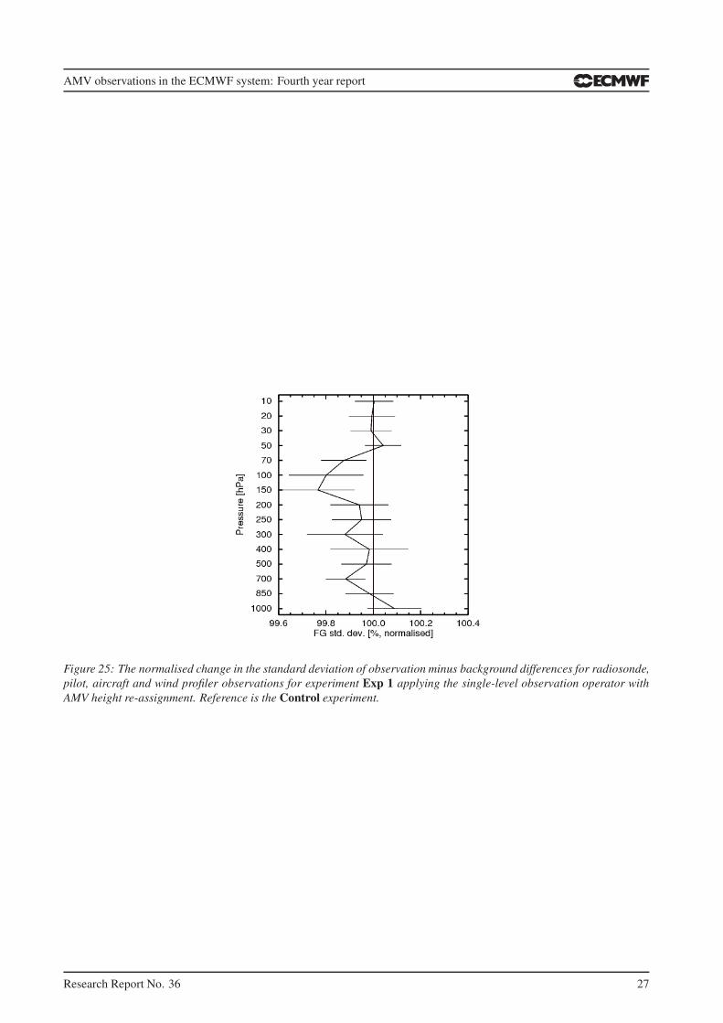
The most promising results are seen for the Exp 1 where a traditional single-level observation operator is used

together with the height re-assignment. Figure 25 shows the normalised change in the standard deviation of

background differences for radiosonde, pilot, aircraft and wind profiler observations. The observation fit is

improved at almost all levels indicating that the observations agree better with the model first guess.

Figure 26 shows the normalised difference in vector wind RMS error for 48-hour forecasts for Exp 1 (upper

panel), Exp 2 (middle panel) and Exp 3 (lower panel). The verification has been done against each experiment’s

own analysis. In general, taking into account the systematic height errors for AMVs has a positive impact on

the forecasts, especially in the tropics. The experimentation with layer averaging gives more mixed results.

For both experiments using the layer averaging observation operator a statistically significant negative impact



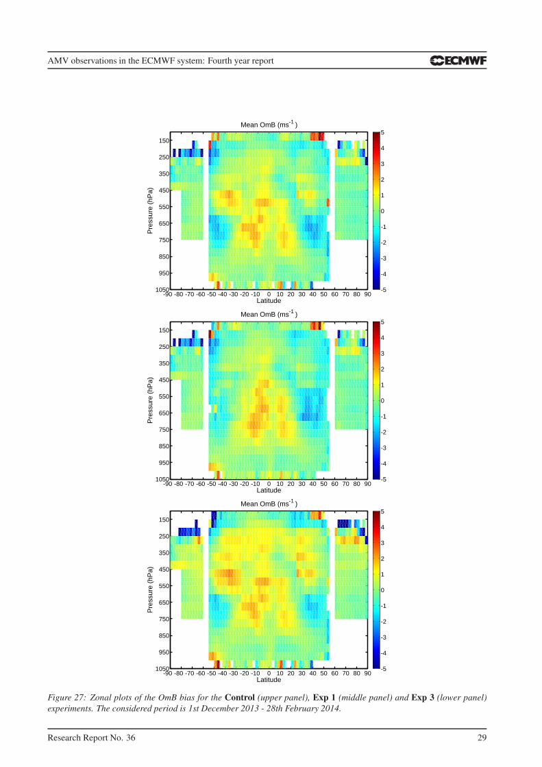
is seen between 30◦S and 30◦N above 400 hPa. Figure 27 shows the zonal plots of OmB wind speed bias

for the Control (upper panel), Exp 1 (middle panel) and Exp 2 (lower panel). Generally there is a positive

speed bias in the tropics at mid and high levels, i.e. the observed wind is on average stronger than the model

counterpart. Using the layer averaging observation operator increases the magnitude of this bias. The Met

Office has seen similar issues in their preliminary work (Mary Forsythe, personal communication). For Exp 2

where layer averaging is done 40 hPa below the assigned AMV pressure indications of positive impact are seen

at low levels (Fig. 26). Single observation experiments have confirmed that averaging below the assigned AMV

pressure shifts the maximum analysis increment downwards and thus has an effect similar to re-assigning the

AMV pressure lower in the atmosphere than the assigned pressure.

It can be concluded that the results from the first experiments indicate clear benefits from taking into account

the systematic height errors. The impact of using layer averaging observation operator is more mixed. Further

investigations are ongoing.

-100 -50 0 50 100

1000

800

600

400

200

0

Mean difference (hPa)

Pre

ssur

e (h

Pa)

IR

MET-10, CCCGOES-15, EBBTMTSAT-2, EBBT

Figure 24: Mean difference of assigned AMV pressure minus model best-fit pressure at different pressure levels for

Meteosat-10 AMVs utilising Cross Correlation Contribution (CCC) height assignment (black line) and for GOES-15

(blue line) and MTSAT-2 (red line) AMVs with equivalent black-body temperature (EBBT) height assignment.



Figure 25: The normalised change in the standard deviation of observation minus background differences for radiosonde,

pilot, aircraft and wind profiler observations for experiment Exp 1 applying the single-level observation operator with

AMV height re-assignment. Reference is the Control experiment.



Figure 26: Zonal plots of the normalised difference (experiment minus control) of the RMS wind error for the 48-hour

forecasts for the experiment applying the single-level observation operator with AMV height re-assignment (left panel),

40 hPa bocxcar averaging below the assigned height (middle panel) and 120 hPa centred averaging (right panel). The

control experiment uses the traditional single-level observation operator. The considered period is 1st December 2013 -

28th February 2014.



-90 -80 -70 -60 -50 -40 -30 -20 -10 0 10 20 30 40 50 60 70 80 901050

950

850

750

650

550

450

350

250

150

Latitude

Pre

ssur

e (h

Pa)

Mean OmB (ms-1 )

-5

-4

-3

-2

-1

0

1

2

3

4

5

-90 -80 -70 -60 -50 -40 -30 -20 -10 0 10 20 30 40 50 60 70 80 901050

950

850

750

650

550

450

350

250

150

Latitude

Pre

ssur

e (h

Pa)

Mean OmB (ms-1 )

-5

-4

-3

-2

-1

0

1

2

3

4

5

-90 -80 -70 -60 -50 -40 -30 -20 -10 0 10 20 30 40 50 60 70 80 901050

950

850

750

650

550

450

350

250

150

Latitude

Pre

ssur

e (h

Pa)

Mean OmB (ms-1 )

-5

-4

-3

-2

-1

0

1

2

3

4

5

Figure 27: Zonal plots of the OmB bias for the Control (upper panel), Exp 1 (middle panel) and Exp 3 (lower panel)

experiments. The considered period is 1st December 2013 - 28th February 2014.



Acknowledgements

Kirsti Salonen is funded by the EUMETSAT fellowship programme.

References

Carranza, M., Borde, R., Doutriaux-Boucher, M., 2014. Recent changes in the derivation of geostationary atmo-

spheric motion vectors at EUMETSAT. Proceedings of the 12th International Wind Workshop, Copenhagen,

Denmark, 16-20 June 2014.

Cotton, J., 2013. Comparing AMVs over Indian Ocean. Available online at

http://nwpsaf.eu/monitoring/amv/investigations/iodc/nwpsaf mo tr 028.pdf.

Deb, S., 2012. Multiplet based technique to derive atmospheric winds from Kalpana-1. Proceedings of the 11th

International Wind Workshop, Auckland, New Zealand, 20-24 February 2012.

Folger, K., Weissmann, M., 2014. Height correction of atmospheric motion vectors using satellite lidar obser-

vations from CALIPSO. JAMC 53, 18091819.

Forsythe, M., Saunders, R., 2008. AMV errors: a new approach in NWP. Proceedings of the 9th International

Wind Workshop, Annapolis, Maryland, USA, 14-18 April 2008 EUMETSAT P.51.

Hernandez-Carrascal, A., Bormann, N., 2014. Atmospheric motion vectors from model simulations. Part II:

Interpretation as spatial and vertical averages of wind and role of clouds. J. Appl. Meteor. Climatol. 53,

65–82.

Peubey, C., McNally, A., 2009. Characterization of the impact of geostationary clear-sky radiances on wind

analyses in a 4D-Var context. QJRMS 135, 18631876.

Salonen, K., Bormann, N., 2013a. Atmospheric Motion Vector observations in the ECMWF system: Third year

report. EUMETSAT/ECMWF Felloship Programme Research Report No.32.

Salonen, K., Bormann, N., 2013b. Winds of change in the use of Atmospheric Motion Vectors in the ECMWF

system. ECMWF Newsletter 136, 23–27.

Salonen, K., Cotton, J., Bormann, N., Forsythe, M., 2015. Characterising AMV height assignment error by

comparing best-fit pressure statistics from the Met Office and ECMWF data assimilation systems. JAMC 54,

225–242.

Velden, C., S., Bedka, K., M., 2009. Identifying the uncertainty in determining satellite-derived atmospheric

motion vector height attribution. J. Applied Meteorology and Climatology 2, 380–392.

Weissmann, M., Folger, K., Lange, H., 2013. Height correction of atmospheric motion vectors using lidar

observations. JAMC 52, 1868–1877.

Zhang, X., Xu, J., Zhang, Q., 2014. Status of operational AMVs from FY-2 satellites since the 11th wind

workshop. Proceedings of the 12th International Wind Workshop, Copenhagen, Denmark, 16-20 June 2014.


Date post:	19-Apr-2018
Category:	Documents
Upload:	leminh
View:	218 times
Download:	5 times

Atmospheric Motion Vector observations in the … operated Kalpana-1 and INSAT-3D. The INSAT-3D AMVs...

Documents