Atmospheric Properties from the 2006 Niamey …. Mather et al., September 2008, DOE/SC-ARM/P-08-018...

DOE/SC-ARM/P-08-018

Atmospheric Properties from the 2006 Niamey Deployment and Climate Simulation with a Geodesic Grid Coupled Climate Model Fourth Quarter 2008 ARM and Climate Change Prediction Program Report J. Mather/Pacific Northwest National Laboratory D. Randall/Colorado State University C. Flynn/Pacific Northwest National Laboratory September 2008 Work supported by the U.S. Department of Energy, Office of Science, Office of Biological and Environmental Research

DISCLAIMER This report was prepared as an account of work sponsored by the U.S. Government. Neither the United States nor any agency thereof, nor any of their employees, makes any warranty, express or implied, or assumes any legal liability or responsibility for the accuracy, completeness, or usefulness of any information, apparatus, product, or process disclosed, or represents that its use would not infringe privately owned rights. Reference herein to any specific commercial product, process, or service by trade name, trademark, manufacturer, or otherwise, does not necessarily constitute or imply its endorsement, recommendation, or favoring by the U.S. Government or any agency thereof. The views and opinions of authors expressed herein do not necessarily state or reflect those of the U.S. Government or any agency thereof.

J. Mather et al., September 2008, DOE/SC-ARM/P-08-018

iii

Acknowledgments

The authors would specifically like to thank the aerosol observing system (AOS) mentor, Anne Jefferson, for her hard work maintaining the AOS under adverse conditions. We would also like to recognize both Anne Jefferson and John Ogren for the expertise and critical insight that helped to define this data product.


iv

Contents 1. Introduction ........................................................................................................................................... 1

2. Niamey Aerosol and Dust Properties .................................................................................................... 1

2.1 Aerosol Instrumentation and Measurements ............................................................................. 1

2.2 Niamey Local Conditions .......................................................................................................... 2

2.3 Algorithm and Method .............................................................................................................. 3

2.4 Data Product Description .......................................................................................................... 7

3. Results of a Decade-long Control Simulation Using Geodesic Grid Coupled Climate Model at a Resolution ~ 250 km, Including a Comparison with Observations ...................................................... 8

3.1 Model Description ..................................................................................................................... 8

3.2 Initial Testing .......................................................................................................................... 10

3.2.1 Tests of the Atmosphere and Land-Surface Models with Prescribed Sea-Surface Temperatures and Sea Ice ........................................................................................... 10

3.2.2 Tests of the Ocean and Sea Ice Models with Prescribed Atmospheric Forcing ......... 10

3.3 A Ten-year Coupled Simulation .............................................................................................. 11

3.4 Summary and Conclusions ...................................................................................................... 14

3.5 References ............................................................................................................................... 15

Figures 1. Measurement alternates between 1-micron and 10-micron size-cut ................................................ 2

2. Correlation between AOS total scattering, green, 10-micron cut-off versus the met tower visibility sensor ................................................................................................................................ 4

3. Correlation between AOS total scattering with 1-micron and 10-micron size cuts ......................... 4

4. dentification of smoke from interpolated SSA ................................................................................ 5

5. Identification of dust event with interpolated SSA .......................................................................... 6

6. Identified dust events throughout the Niamey deployment ............................................................. 7

7. The process used to create a geodesic grid, by starting from an icosahedron. ................................. 8

8. The observed and simulated annual-mean distributions of total precipitation .............................. 10

9. January and July sea surface temperature ...................................................................................... 11

10. Simulated January sea surface temperature patterns for years 1 and 10 of the coupled run. ......... 12

11. Simulated January sea ice concentration for years 1 and 10 of the coupled run ............................ 13

12. Observed and simulated January precipitation rates. ..................................................................... 14


1

1. Introduction

In 2008, the Atmospheric Radiation Measurement (ARM) Program and the Climate Change Prediction Program (CCPP) have been asked to produce joint science metrics. For CCPP, the metrics will deal with a decade-long control simulation using geodesic grid-coupled climate model. For ARM, the metrics will deal with observations associated with the 2006 deployment of the ARM Mobile Facility (AMF) to Niamey, Niger. Specifically, ARM has been asked to deliver data products for Niamey that describe cloud, aerosol, and dust properties. The first quarter milestone was the initial formulation of the algorithm for retrieval of these properties. The second quarter milestone included the time series of ARM-retrieved cloud properties and a year-long CCPP control simulation. The third quarter milestone included the time series of ARM-retrieved aerosol optical depth and a three-year CCPP control simulation. This final fourth quarter milestone includes the time-series of aerosol and dust properties and a decade-long CCPP control simulation.

2. Niamey Aerosol and Dust Properties

Niamey is located in the southwest corner of Niger in sub-Saharan western Africa. The Saharan Desert covers the northern half of Niger. The seasons in Niamey are divided between monsoon (roughly May through October) and dry (November through April). This seasonal pattern is driven by the annual movement of the Inter-Tropical Front (ITF; Slingo et al., 2008). The ITF represents the division between hot, dry, dusty Saharan air in the northeast and moisture-laden air from the tropical Atlantic in the southwest. As this diagonally-oriented front moves northwards over Niamey, it brings moist air and the monsoon season. As it recedes southwards, the dry season returns. Irrespective of season, however, conditions at the surface are dominated by the two main types of aerosol: dust due to the proximity of the Sahara Desert, and soot from local and regional biomass burning. The purpose of this new data product is to identify when the local conditions are dominated by the dust component so that the properties of the dust events can be further studied.

2.1 Aerosol Instrumentation and Measurements

The aerosol observing system (AOS) is the primary ARM platform for in situ aerosol measurements at the surface (Sheridan et al., 2001). The AOS simultaneously measures aerosol optical scattering and absorption coefficients at three wavelengths (nominally red, green, and blue) for both dried and humidified aerosols. The measurement sequence alternates between a maximum particle size cut-off of 1 and 10 um as illustrated in Figure 1. The top panels show aerosol scattering and absorption coefficients (on the left and right, respectively) measured with the 10-micron size cut-off. The middle panels show the same measurements but with the 1-micron size cut-off. It is apparent from these two panels that the feature having a relative maximum on the left half of the plot is composed of fairly large particles, since it shows up mainly in the 10-um measurement and much less in the 1-um measurement. Presumably this is dust. In contrast, the feature with relative maximum at 32.8 shows up more strongly in the 1-um measurement. It also has a stronger signature in the right-hand panels, which show absorption, so this feature is composed of fine soot.


2

Figure 1: Measurement alternates between 1-micron and 10-micron size-cut. Right panels show scattering, left panels show absorption. Bottom panels show the submicron ratio inferred from the top and middle panels.

From the collection of extensive aerosol properties a number of intensive properties are computed, including aerosol single scattering albedo (SSA), angstrom exponents for scattering and absorption, submicron fractions of scattering and absorption (shown in Figure 1), backscattering fraction, and asymmetry parameter.

Additional measurements include the total particle number concentration from an optical particle counter, and the rate of condensation nucleation as a function of super-saturation level. In addition to the AOS, the Niamey site included a standard met tower with temperature, pressure, RH, and winds, but it also included a measurement of local visibility, which turned out to be valuable.

Finally, a Multi-Filter Rotating Shadowband Radiometer (MFRSR) was operated to retrieve aerosol optical depth. The MFRSR AOD product (described and delivered in the previous third quarter metric) also is provided here as it pertains to aerosol properties in the atmospheric column.

2.2 Niamey Local Conditions

The surface conditions in Niamey show much higher aerosol loading than previous ARM AOS deployments. For example, at the ARM Climate Research Facility (ACRF) Southern Great Plains (SGP) site, the average total scattering coefficient is about 47 Mm-1 and the average absorption coefficient is about 2.5 Mm-1(Sheridan et al., 2001; Delene and Ogren, 2001). Even after excluding major dust events during the dry season in Niamey, the average of total scattering is more than 120 Mm-1 with daily peaks routinely exceeding 150 Mm-1. The dry season daily-averaged absorption coefficient (excluding major dust events) is about 12 Mm-1 with daily peaks in excess of 15 Mm-1. Isolated dust storms generated hourly-averaged total scattering coefficients in excess of 3000 Mm-1 and absorption coefficients greater than 300 Mm-1.


3

These conditions are very challenging for autonomous in situ aerosol measurements. For example, the porous filters used in the absorption coefficient measurements become saturated, more quickly under higher aerosol loads. When the filters are saturated the absorption measurements are inaccurate so the filters need more frequent replacement. In general, dirty operating environments cause more wear and tear on moving equipment. Nevertheless, the AOS operated as designed over both the pre-monsoon and post-monsoon dry seasons. It did experience some difficulties toward the end of the first dry season and was entirely down for the first half of the wet season.

2.3 Algorithm and Method

Distinguishing Characteristics for Dust and Soot: Both dust storms and smoke from biomass burning will exhibit high aerosol total scattering coefficient values. However, the dust storms at Niamey have several characteristics that will be used to identify these events and distinguish them from biomass burning. The most important of these is the large size of the dust particles and the degree to which the large particles dominate the total aerosol scattering measurements. Almost as important is the observation that, while the dust particles have significant absorption (SSA < .9 for large particle scattering fraction), they are not as dark as the soot from biomass burning (SSA < ~0.8).

From these observed characteristics we define the following tests:

1. Total scattering for green with 10-um cut-off > 200 1/Mm

2. Scattering Angstrom exponent (blue-green) with 10-um cut-off < 0.5

3. Scattering Angstrom exponent (blue-green) with 1-um cut-off < 1

4. Submicron fraction of scattering for green < 0.25

5. Submicron fraction of scattering for green < 0.6

6. Single scattering albedo for green with 10 um impactor > 0.89.

As noted earlier, however, not all of these measurements were available all the time. In fact, critical measurements are missing for as many as 100 days. The criteria above are listed in order of importance to the identification algorithm. To provide a more continuous time series, the following adaptations were applied to provide alternate input for these critical tests.

Recovery of Missing Total Scattering Coefficients from Visibility: The AOS was inoperable for a period of 98 days extending from May 7 to August 13. Coincidentally, May 7 marks the passing of the ITF and the nominal start of the monsoon season. Essentially the AOS missed the first half of the monsoon cycle, but it was operational for the second half. Figure 2 shows the correlation between the total scattering coefficients and the visibility sensor on the met tower. The regression line was used to generate a proxy for the AOS total scattering for use in the identification algorithm only during the first half of the monsoon season when the AOS total scattering coefficients are unavailable.


4

Figure 2: Correlation between AOS total scattering, green, 10-micron cut-off versus the met tower visibility sensor. The red line is a linear regression used to infer the total scattering coefficient from the visibility measurement.

Recovery of Alternate Size cut-off Measurements: Due to the difficult operating environment, there were periods when the impactor used to select the maximum particle cut-off size would fail to alternate, leaving the size cut-off fixed an extended time. This situation impacts criteria 4 and 5 in the identification algorithm since the submicron scattering fractions would be unavailable. From the most recent measurements, when both size cuts were operating, we obtained empirical relationships such as that shown in Figure 3, permitting us to infer measurements at one size cut from another.

Figure 3: Correlation between AOS total scattering with 1-micron and 10-micron size cuts. The horizontal axis is the total scattering coefficient for green with a 10-micron size cut-off. The vertical axis is the same quantity with a 1-micron size cut-off. The red line is a linear regression between the two.


5

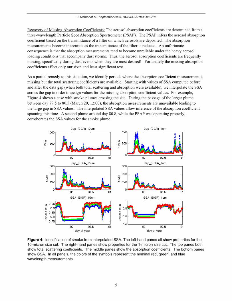
Recovery of Missing Absorption Coefficients: The aerosol absorption coefficients are determined from a three-wavelength Particle Soot Absorption Spectrometer (PSAP). The PSAP infers the aerosol absorption coefficient based on the transmittance of a filter on which aerosols are deposited. The absorption measurements become inaccurate as the transmittance of the filter is reduced. An unfortunate consequence is that the absorption measurements tend to become unreliable under the heavy aerosol loading conditions that accompany dust storms. Thus, the aerosol absorption coefficients are frequently missing, specifically during dust events when they are most desired! Fortunately the missing absorption coefficients affect only our sixth and least significant test.

As a partial remedy to this situation, we identify periods where the absorption coefficient measurement is missing but the total scattering coefficients are available. Starting with values of SSA computed before and after the data gap (when both total scattering and absorption were available), we interpolate the SSA across the gap in order to assign values for the missing absorption coefficient values. For example, Figure 4 shows a case with smoke plumes crossing the site. During the passage of the larger plume between day 79.5 to 80.5 (March 20, 12:00), the absorption measurements are unavailable leading to the large gap in SSA values. The interpolated SSA values allow inference of the absorption coefficient spanning this time. A second plume around day 80.8, while the PSAP was operating properly, corroborates the SSA values for the smoke plume.

Figure 4: Identification of smoke from interpolated SSA. The left-hand panes all show properties for the 10-micron size cut. The right-hand panes show properties for the 1-micron size cut. The top panes both show total scattering coefficients. The middle panes show the absorption coefficients. The bottom panes show SSA. In all panels, the colors of the symbols represent the nominal red, green, and blue wavelength measurements.


6

As another example, Figure 5 illustrates a multi-day dust event where the PSAP filter was replaced several times. Note that the SSA tracks fairly well throughout the event. Just after day 72, some smoke plumes appear yielding short-lived reductions in SSA.

Figure 5: Identification of dust event with interpolated SSA. Aerosol properties with a 1-micron and 10-micron size cut are shown in the right and left hand panes, respectively. The top panes both show total scattering coefficients. The middle panes show the absorption coefficients. The bottom panes show SSA. In all panels, the colors of the symbols represent the nominal red, green, and blue wavelength of the measurements.

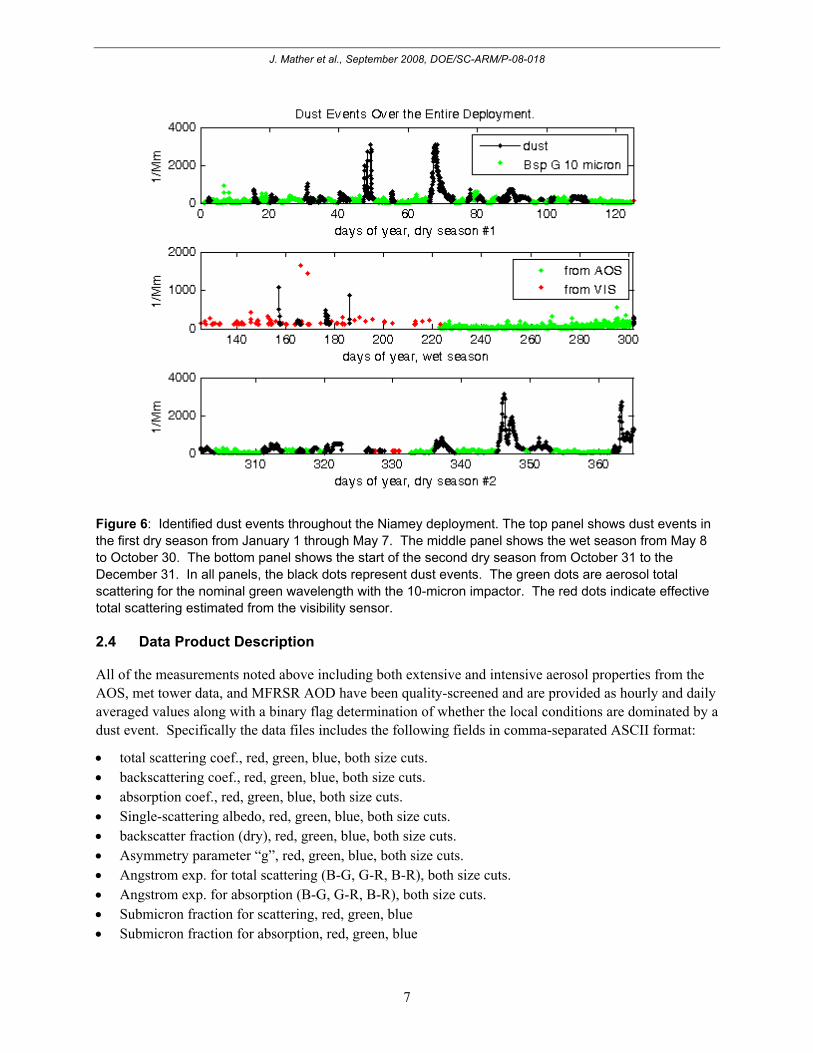
Dust event identification: After assembling the complete data record and applying the adaptations described above to provide a more complete time series, the hourly-averaged data were assessed according to the six test conditions. Times for which all of the conditions 1-4 or conditions 1-3 and 5-6 are met are considered to be dominated by dust. To eliminate momentary data spikes and short-lived events such as gust fronts, we flag only those periods dominated by dust for several consecutive hours as dust events. We have identified 75 days as having local conditions dominated by dust, shown in Figure 6. When consecutive days are counted as a single event, this yields a total of 30 discrete dust events.


7

Figure 6: Identified dust events throughout the Niamey deployment. The top panel shows dust events in the first dry season from January 1 through May 7. The middle panel shows the wet season from May 8 to October 30. The bottom panel shows the start of the second dry season from October 31 to the December 31. In all panels, the black dots represent dust events. The green dots are aerosol total scattering for the nominal green wavelength with the 10-micron impactor. The red dots indicate effective total scattering estimated from the visibility sensor.

2.4 Data Product Description

All of the measurements noted above including both extensive and intensive aerosol properties from the AOS, met tower data, and MFRSR AOD have been quality-screened and are provided as hourly and daily averaged values along with a binary flag determination of whether the local conditions are dominated by a dust event. Specifically the data files includes the following fields in comma-separated ASCII format:

• total scattering coef., red, green, blue, both size cuts. • backscattering coef., red, green, blue, both size cuts. • absorption coef., red, green, blue, both size cuts. • Single-scattering albedo, red, green, blue, both size cuts. • backscatter fraction (dry), red, green, blue, both size cuts. • Asymmetry parameter “g”, red, green, blue, both size cuts. • Angstrom exp. for total scattering (B-G, G-R, B-R), both size cuts. • Angstrom exp. for absorption (B-G, G-R, B-R), both size cuts. • Submicron fraction for scattering, red, green, blue • Submicron fraction for absorption, red, green, blue


8

• CCN fraction at supersaturation of 0.5% • CCN fraction at supersaturation of 0.7% • CCN fraction at supersaturation of 0.9% • CCN fraction at supersaturation of 1.2% • MFRSR aerosol optical depth, 415 nm • MFRSR aerosol optical depth, 500 nm • MFRSR aerosol optical depth, 615 nm • MFRSR aerosol optical depth, 673 nm • MFRSR aerosol optical depth, 870 nm • MFRSR angstrom exponent, 500nm-870nm • Visibility from met tower, 10 minute avg. • Wind speed from met tower, vector avg. • Wind dir from met tower, vector avg. • Wind speed, northerly component. • Wind speed, easterly component • Ambient temperature • Ambient relative humidity • Ambient pressure.

3. Results of a Decade-long Control Simulation Using Geodesic Grid Coupled Climate Model at a Resolution ~ 250 km, Including a Comparison with Observations

3.1 Model Description

The Coupled Colorado State Model (CCoSM) is a climate model in which each component is discretized on a geodesic grid (Figure 7). A geodesic grid consists of hexagons and pentagons. The grid-cells are relatively uniform across the globe, varying in area by only 5%, and the grid is quasi-isotropic. The distinct climate components in CCoSM are the atmosphere, ocean and sea ice, and their coupling is coordinated by a coupler component that computes the interfacial fluxes and PBL physics.

Figure 7: The process used to create a geodesic grid, by starting from an icosahedron.


9

The geodesic grid can be decomposed into logically rectangular subdomains, which are used to do memory allocation on a computer. Each subdomain can be decomposed in two dimensions. The model runs in a multiple-processor environment using the message passing interface (MPI).

The atmosphere sub-model includes prognostic equations for potential temperature, vorticity and divergence, surface pressure, specific humidity, cumulus kinetic energy (CKE), mixing ratios of cloud water, cloud ice, rain and snow, and the planetary boundary layer (PBL) depth. The discretization of the advection is highly conservative. The vertical coordinate is a generalized sigma coordinate, in which the PBL top is a coordinate surface. There are 29 layers, with the model top at 1 mb.

Deep moist convection is parameterized using a modified Arakawa-Schubert scheme with ice, prognostic CKE, cumulus friction, and multiple cloud bases (Pan and Randall, 1998; Ding and Randall, 1998). The large-scale cloud microphysical scheme is the one developed by Fowler et al. (1996), with cumulus detrainment as a source of cloud water and/or ice. The radiation is the Stephens parameterization. Gravity-wave drag is parameterized with a simple Palmer-like scheme (Palmer et al., 1986). Further details are given by Ringler et al. (2000) and Randall et al. (2002).

The ocean sub-model has prognostic equations for momentum, temperature, salinity and the free surface height. Depth is used as the vertical coordinate, with 33 layers. Horizontal transport is done by monotone flux-corrected transport, and vertical transport by monotone remapping. KPP (Large et al., 1994) is used to parameterize the ocean boundary-layer turbulence and convection.

The sea ice sub-model predicts ice concentration, volume and energy content. There are four ice layers, and snow is accumulated on the ice. The dynamics are based on the elastic-viscous-plastic rheology (Hunke and Dukowicz, 1997). The thermodynamics are based on Semtner (1976). Flux-corrected transport is used to advect the ice.

In addition, CCoSM includes a sub-model for land-surface processes, SiB2, which was developed by Sellers et al. (1996). SiB2 includes parameterizations of canopy physiological responses (photosynthesis, stomatal conductance), and was designed to utilize satellite measurements for many of the important vegetation boundary conditions such as fraction of shortwave radiation absorbed, leaf area index, albedo and roughness.

The integrations of these several components are coordinated by a software component called a coupler. On every time step, variables needed to compute the fluxes of mass, momentum and energy between components are passed to the coupler. The coupler computes these fluxes and sends them to the components. To deal with possible differences in resolution, a conservative interpolation is performed using SCRIP, which was developed at the Los Alamos National Laboratory (Jones, 1999). The PBL parameterization, which determines the surface fluxes, PBL-top entrainment rate, and PBL-cloudiness, is implemented in the coupler.

The coupler also can be used to replace climate components with prescribed data. For instance, the dynamic ocean and sea ice modules can be replaced with prescribed sea surface temperature and ice cover to drive the atmosphere; the dynamic atmosphere can be replaced with prescribed surface air conditions, radiative fluxes and precipitation to drive the ocean. In the tests described below, the coupler was used in this way.


10

3.2 Initial Testing

3.2.1 Tests of the Atmosphere and Land-Surface Models with Prescribed Sea-Surface Temperatures and Sea Ice

The atmosphere and land-surface models have been subjected to many tests over a period of years. In a particularly important test, we performed an Atmospheric Model Intercomparison Project (AMIP) simulation (Gates, 1992), in which observed sea-surface temperatures and sea-ice distributions for the years 1979-1988 were prescribed as input. The model results were then analyzed to see if the simulated atmosphere and land surface respond to the year-to-year variations in the sea-surface temperature and sea ice in the same way as observed in the real world. We used 250 km grid spacing. An example of the results from our AMIP run is shown in Figure 8, which compares simulated and observed annual-mean total precipitation.

3.2.2 Tests of the Ocean and Sea Ice Models with Prescribed Atmospheric Forcing

To test the ocean and sea-ice models, we have performed simulations in which the ocean and sea ice are “forced” with prescribed atmospheric data. The initial conditions for the ocean are rest (no currents), with temperature and salinity from the Levitus (1982) January climatology. The sea ice is initialized with a realistic January 1 distribution of 95% (90%) concentration for the northern (southern) hemisphere, with a thickness of 2 m (1m), 0.2m of snow cover, and an ice-surface temperature of -1 °C, and interior ice snow energies consistent with temperatures of 0 °C. The atmospheric driving data are from the ERA-40 reanalysis (Uppala et al., 1999), interpolated to the geodesic grid. The model was integrated for four years with a 200 s time step for all components. We used 250 km grid-spacing.

Figure 8: The observed (top panel) and simulated (bottom panel) annual-mean distributions of total precipitation. The simulation is based on an AMIP run, as described in the text.


11

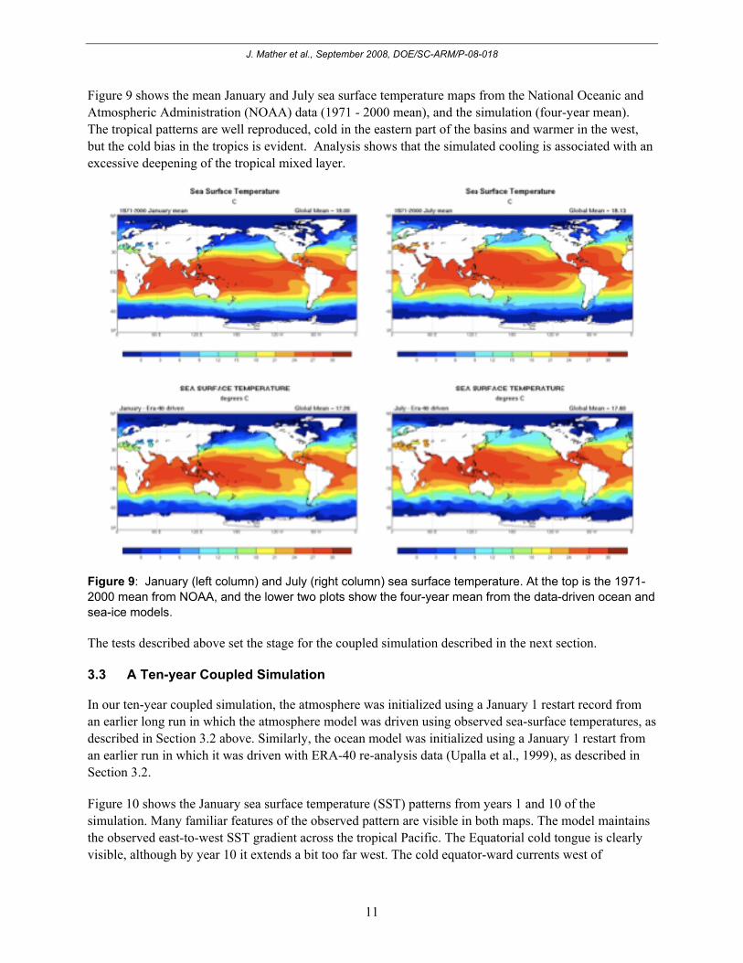
Figure 9 shows the mean January and July sea surface temperature maps from the National Oceanic and Atmospheric Administration (NOAA) data (1971 - 2000 mean), and the simulation (four-year mean). The tropical patterns are well reproduced, cold in the eastern part of the basins and warmer in the west, but the cold bias in the tropics is evident. Analysis shows that the simulated cooling is associated with an excessive deepening of the tropical mixed layer.

Figure 9: January (left column) and July (right column) sea surface temperature. At the top is the 1971-2000 mean from NOAA, and the lower two plots show the four-year mean from the data-driven ocean and sea-ice models.

The tests described above set the stage for the coupled simulation described in the next section.

3.3 A Ten-year Coupled Simulation

In our ten-year coupled simulation, the atmosphere was initialized using a January 1 restart record from an earlier long run in which the atmosphere model was driven using observed sea-surface temperatures, as described in Section 3.2 above. Similarly, the ocean model was initialized using a January 1 restart from an earlier run in which it was driven with ERA-40 re-analysis data (Upalla et al., 1999), as described in Section 3.2.

Figure 10 shows the January sea surface temperature (SST) patterns from years 1 and 10 of the simulation. Many familiar features of the observed pattern are visible in both maps. The model maintains the observed east-to-west SST gradient across the tropical Pacific. The Equatorial cold tongue is clearly visible, although by year 10 it extends a bit too far west. The cold equator-ward currents west of


12

North America and South America are clearly visible. The western Pacific Warm Pool is maintained at year 10, although its shape has changed and it is somewhat weaker. Overall, the simulated SST has cooled by about 0.3 K over the simulated decade. This drift of the simulation is not extreme, but will bear watching in longer tests.

Figure 10: Simulated January sea surface temperature patterns for years 1 and 10 of the coupled run.

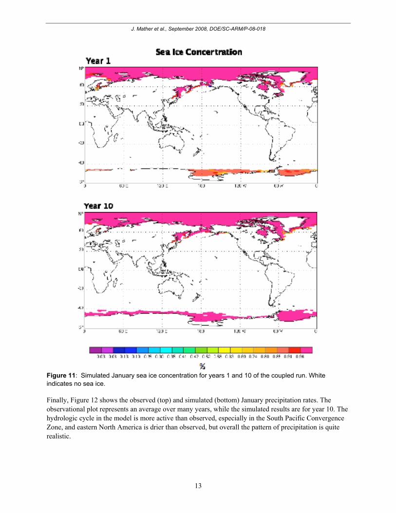
Figure 11 shows the simulated January sea ice concentration for years 1 and 10. The model does a good job of simulating the observed patterns. The sea ice has expanded somewhat in the Southern Hemisphere, but is remarkably stable in the Northern Hemisphere.


13

Figure 11: Simulated January sea ice concentration for years 1 and 10 of the coupled run. White indicates no sea ice.

Finally, Figure 12 shows the observed (top) and simulated (bottom) January precipitation rates. The observational plot represents an average over many years, while the simulated results are for year 10. The hydrologic cycle in the model is more active than observed, especially in the South Pacific Convergence Zone, and eastern North America is drier than observed, but overall the pattern of precipitation is quite realistic.


14

Figure 12: Observed and simulated January precipitation rates.

3.4 Summary and Conclusions

We have created the world’s first geodesic ocean model, including a sea-ice submodel, and have coupled it with geodesic atmosphere and land-surface models, to form the first geodesic coupled climate model. The component models were tested before coupling, by driving them with observations.

The coupled model maintains a fairly realistic state after 10 simulated years. There is a slow drift towards cooler SSTs, but it is not known whether this would continue, equilibrate, or reverse itself in a longer


15

simulation. The sea ice distribution is stable, and the shape of the simulated precipitation pattern is good, although the hydrologic cycle is more active than observed.

Future work will include testing the model at higher horizontal resolution -- particularly the ocean component.

3.5 References

Delene, DJ, and JA Ogren. 2001. “Variability of aerosol optical properties at four North American surface monitoring sites.” J. Geophysical Res.,106,No 18,20735-20747

Ding, P, and DA Randall. 1998. “A cumulus parameterization with multiple cloud base levels.” J. Geophys. Res. 103, 11341-11354.

Fowler, LD, DA Randall, and SA Rutledge. 1996. “Liquid and ice cloud microphysics in the CSU general circulation model. part 1: model description and simulated microphysical processes.” J. Climate. 9, 489-529.

Gates, WL. 1992. “AMIP: The atmospheric model intercomparison project.” Bull. Amer. Meteor. Soc., 73, 1962 - 1970.

Heikes, RP, and DA Randall. 1995. “Numerical integration of the shallow water equations on a twisted icosahedral grid. Part I: Basic design and results of tests.” Mon. Wea. Rev. 123, 1862-1880.

Hunke, EC, and JK Dukowicz. 1997. “An elastic-viscous-plastic model for sea ice dynamics.” J. Phys. Oceanogr. 27, 1849-1867.

Jones, PW. 1999. “First- and second-order conservative remapping schemes for grids in spherical coordinates.” Mon. Wea. Rev. 127, 2204-2210.

Large, WG, JC McWilliams, and SC Doney. 1994. “Oceanic vertical mixing: a review and a model with a nonlocal boundary layer parameterization.” Rev. Geophys. 32, 363-403.

Levitus, S. 1982. “Climatological atlas of the world oceans.” NOAA Prof. Paper 13, U. S. Govt. Printing Office, Washington, D.C.

Michalsky, JJ , JA Schlemmer, WE Berkheiser, JL Berndt, LC Harrison, NS Laulainen, NR Larson, and JC Barnard. 2001. "Multiyear measurements of aerosol optical depth in the Atmospheric Radiation Measurement and Quantitative Links Programs." J. Geophys. Res. 106: 12,099.

Palmer, TN, GJ Shutts, and R Swinbank. 1986. “Alleviation of a systematic westerly bias in general circulation and numerical weather prediction models through an orographic gravity wave drag parametrization.” Quart. J. R. Met. Soc. 112, 1001-1039.

Pan, D-M, and DA Randall. 1998. “A cumulus parameterization with a prognostic closure.” Quart. J. Roy. Met. Soc. 124, 949-981.


16

Randall, DA, TD Ringler, RP Heikes, P Jones, and J Baumgardner. 2002. “Climate modeling with spherical geodesic grids.” Computing in Science Engr. 4, 32-41.

Reynolds, RW, and TM Smith. 1995. “A high resolution global sea surface temperature climatology.” J. Climate. 8, 1571-1583.

Ringler, TD, RP Heikes, and DA Randall. 2000. “Modeling the atmospheric general circulation using a spherical geodesic grid: A new class of dynamical cores.” Mon. Wea. Rev. 128, 2471-2490.

Russell, PB, JM Livingston, O Dubovik, SA Ramirez, J Wang, J Redemann, B Schmid, M Box and BN Holben. 2004. “Sunlight transmission through desert dust and marine aerosols: Diffuse light corrections to Sun photometry and pyrheliometery.” J. Geophys. Res., 109, D08207, doi:10.1029/2003JD004292.

Sellers, PJ, DA Randall, GJ Collatz, J Berry, C Field, DA Dazlich, C Zhang, and L Bounoua. 1996. “A revised land-surface parameterization (SiB2) for atmospheric GCMs. part 1: model formulation.” J. Climate. 9, 676-705.

Semtner, AJ Jr. 1976. “A Model for the thermodynamic growth of sea ice in numerical investigations of climate.” J. Phys. Oceanogr. 6, 379-389.

Sheridan, PJ, DJ Delene, and JA Ogren. “Four years of continuous surface aerosol measurements from the Department of Energy’s Atmospheric Radiation Measurement Program Southern Great Plains Cloud and Radiation Testbed site.” J. Atmos. Sci., 59, 1135-1150, 2002.

Slingo, A, NA Bharmal, GJ Robinson, JJ Settle, RP Allan, HE Whilte, PJ Lamb, M Issa Lele, DD Turner, S McFarlane, E Kassianov, J Barnard, C Flynn, and M Miller. 2008. “Overview of observations from the RADAGAST experiment in Niamey, Niger: Meteorology and thermodynamic variables,” Geophysical Research Letters, accepted June 23, 2008.

Slingo. A, TP Ackerman, RP Allan, EI Kassianov, SA McFarlane, GJ Robinson, JC Barnard, M Miller, JE Harries, JE Russell, and S. Dewitte. 2006. “Observations of the impact of a major Saharan dust storm on the atmospheric radiation budget.” Geophysical Research Letters, 33, L24817, doi:10.1029/2006GL027869.

Stephens, GL, PM Gabriel, and PT Partain. 2001. “Parameterization of atmospheric radiative transfer. Part I: validity of simple models.” J. Atmos. Sci. 58, 3391 - 3409.

Uppala, S, JK Gibson, M Fiorino, A Hernandez, P Kållberg, X Li, K Onogi, and S Saarinen. 1999. “ECMWF second generation reanalysis—ERA40.” Proc. Second WCRP Int. Conf. on Reanalyses, Wokefield Park, United Kingdom, WCRP. 9–13.

Date post:	21-Jun-2018
Category:	Documents
Upload:	ngotu
View:	213 times
Download:	0 times

Atmospheric Properties from the 2006 Niamey …. Mather et al., September 2008, DOE/SC-ARM/P-08-018...

Documents