Atom-continuum coupled model for thermo-mechanical behavior of materials in micro-nano scales

. Article .Special Issue: Physical Mechanics

SCIENCE CHINAPhysics, Mechanics & Astronomy

June 2012 Vol. 55 No. 6: 1125–1137doi: 10.1007/s11433-012-4765-y

c© Science China Press and Springer-Verlag Berlin Heidelberg 2012 phys.scichina.com www.springerlink.com

Atom-continuum coupled model for thermo-mechanicalbehavior of materials in micro-nano scales

XIANG MeiZhen1*, CUI JunZhi2*, LI BoWen2 & TIAN Xia3

1Laboratory of Computational Physics, Institute of Applied Physics and Computational Mathematics, Beijing 100088, China;2LSEC, ICMSEC, Academy of Mathematics and Systems Sciences, Chinese Academy of Sciences, Beijing 100190, China;

3College of Mechanics and Materials, Hohai University, Nanjing 210098, China

Received March 12, 2012; accepted April 24, 2012

In this paper, an atom-continuum coupled model for thermo-mechanical behaviors in micro-nano scales is presented. A representa-tive volume element consisting of atom clusters is used to represent the microstructure of materials. The atom motions in the RVEare divided into two phases, structural deformations and thermal vibrations. For the structural deformations, nonlinear and nonlocaldeformation at atomic scales is considered. The atomistic-continuum equations are constructed based on momentum and energyconservation law. The non-locality and nonlinearity of atomistic interactions are built into the thermo-mechanical constitutiveequations. The coupled atomistic-continuum thermal-mechanical simulation process is also suggested in this work.

atom-continuum coupled (ACC) model, atomistic model, thermo-mechanical behaviors, nonlocality, multiscale model

PACS number(s): 65.40.-b, 05,10.-a, 31.15.-p

Citation: Xiang M Z, Cui J Z, Li B W, et al. Atom-continuum coupled model for thermo-mechanical behavior of materials in micro-nano scales. Sci China-PhysMech Astron, 2012, 55: 1125–1137, doi: 10.1007/s11433-012-4765-y

1 Introduction

One important goal in materials modeling is to explain andpredict the observed coarse scale phenomena based on theunderstanding of material microstructure. The expression of“microstructure” is a generic denomination for any type ofinternal material structure, not necessarily on the level of mi-crometers. As the scale of microstructure is not very small,the behavior of the materials can be described by the tra-ditional continuum model with spatial variation of materialparameters. In this case, convincing homogenization theoryand related two-scale algorithms have been developed [1–4].But as the scale of microstructure is sufficiently small, thecontinuum description perhaps is no longer adequate, andneeds to be replaced by an atomistic model. An atomisticmodel provides a discrete description of matter. In principle,atomistic models can accurately mode the underlying physi-cal processes at any scale. However, direct atomistic simula-

*Corresponding author (XIANG MeiZhen, email: [email protected]; CUI Jun-Zhi, email: [email protected])

tions are computationally too expensive.The onerous practical limitations of molecular dynamics

simulations and the limited fidelity of traditional continuummodels have inspired researchers to attempt to construct mul-tiscale models. Those can be divided into three classes. Thefirst class is to concurrently couple atomistic and continuummodels, where full atomistic model is only used in localizedregions, in which the atomic-scale dynamics are important,while a continuum simulation is used everywhere else, for ex-ample, the quasi-continuum method [5–7], the bridging scalemethod by Wagner and Liu [8,9], and the bridging domainmethod [10]. The second class of multiscale mode are infor-mation passing models, in which some constitutive data areobtained from local molecular dynamics simulations. Themolecular dynamics simulations are constrained so that theyare consistent with the local macro-state of the system, for ex-ample, the Heterogeneous Multiscale Method (HMM) [11]and the Generalized Mathematical Homogenization (GMH)method [12,13]. The fine and coarse scale models are two-way coupled, which means that the information continuously

1126 Xiang M Z, et al. Sci China-Phys Mech Astron June (2012) Vol. 55 No. 6

transmits between the scales. The third class is general-ized continuum models embedded with atomistic features,where the conservation equations and/or constitutive equa-tions are derived directly from interatomic potentials not in-volving molecular dynamics [5,14–20]. These generalizedcontinuum theories are not impeded by exhaustive computa-tional cost of molecular dynamics, and are potentially suit-able for large-scale problems. The continuum models in thesecond class and third class are used in continuum region ofconcurrently coupled models.

Constructing thermo-mechanical continuum equationsbased on atomistic models has become a significant subjectin recent years. As pointed by Fish et al. [13] and Zhou[21], there are several difficulties that need to be overcome.The first difficulty lies in the fact that continuum and atom-istic models describe thermal phenomenons in different man-ners. In atomistic models, structural deformation and thermalvibration make up the total atomic motion. Molecular dy-namics models explicitly track total displacements. In con-tinuum models, however, these two parts should be treatedseparately. The thermal oscillation of atomic motion is onlyphenomenologically accounted for in the form of heat trans-fer equation. Reconciliation of the differences in the two de-scriptions and, more importantly, the integration of the twoanalysis frameworks for cross-scale characterization are agreat challenge in physics, material science and mechanics.Moreover, in atomistic models, energy transport is carried outthrough “doing work” by forces between atoms. However,in continuum models, the energy transport is separated into“doing-work” and “heat transfer”. The second difficulty isassociated with the formulation of the basic fine-scale modelrequired for developing heat transfer equation. For example,non-metallic solids such as ceramics transfer heat by latticevibrations, while metals transfer heat mainly by collisions offree electrons. Thus, the classical molecular dynamics basedon Newton’s law of atom motions cannot sufficiently describeheat transfer in metals.

Many attempts have been done for linking continuumthermo-mechanical descriptions with fine scale atomisticmodel. Zhou [21] developed a thermo-mechanical equiva-lent continuum (TMEC) theory for continuum descriptions ofmaterial behaviors from pure atomistic simulations. Chen etal. [18,22,23] proposed an approach to define local stress andheat flux for atomistic systems involving three-body forces,based on which they developed a continuum theory that viewsa crystalline material as a continuous collection of latticepoints, while embedded at each point is a group of discreteatoms. Fish et al. [13] derived thermo-mechanical contin-uum equations from Molecular Dynamics equations using theGeneralized Mathematical Homogenization (GMH) theory.In addition, models based on temperature related Cauchy-Born rule (TCB) are widely used for deriving continuumthermo-mechanical equations [24–30]. Those models usetraditional thermo-mechanical continuum conservation equa-tions. A local free energy density is derived based on the

TCB rule and local quasi-harmonic approximation (LQH),and constitutive relation is then derived from the free energydensity formulation. Wang et al. [31] have proposed a groupof statistical thermodynamics methods for the simulations ofnanoscale systems under quasi-static loading at finite temper-ature, that is, molecular statistical thermodynamics (MST)method, cluster statistical thermodynamics (CST) method,and the hybrid molecular/cluster statistical thermodynamics(HMCST) method. One appealing feature of these methodsis their “seamlessness” or consistency in the same underly-ing atomistic model in all regions consisting of atoms andclusters, and hence can avoid ghost forces in the simulation.Another advantage of these methods is their high computa-tional efficiency compariag to direct MD simulations. Othershave presented a multiscale, finite deformation formulationthat accounts for surface stress effects on the coupled thermo-mechanical behavior and properties of nanomaterials [32].Recently, researchers have proposed a thermo-hyperelasticmodel for both the surface and the bulk of nanostructuredmaterials, in which the residual stresses are taken into ac-count [33]. Wagner et al. [34] developed a concurrently cou-pling model for heat transfer in solids. However, their modeldoes not include momentum equations, thus the model cannot capture full thermo-mechanical behaviors of materials.

In our earlier work, an atom-continuum model for dynam-ical problems has been constructed, in which the non-localityand nonlinearity of atomistic interactions are explicitly builtinto the stress-strain relationship [20,35]. The present workis continuing efforts of atomistic-continuum model in micro-nano scales for thermo-mechanical behaviors of materials.In order to overcome the first difficulty mentioned above,atomic displacement is decomposed into two phases, struc-tural deformations and thermal oscillations. Accordingly, theenergy changing rate of atom system is divided into rate ofdoing-work and rate of heat transfer in a proper manner. Thesecondary difficulty lies in the fact that the fundamental finescale model is classical atomistic model, and only lattice vi-bration (phonon) induced heat transfer is accounted for. Themomentum and energy equations are derived directly basedon the atomistic potentials and the internal “icro structures”.Representative volume element (RVE) is used to describe the“micro structures”, and thermo-mechanical constitutive rela-tions are derived based on the free energy analysis of RVEs.The resulted constitutive relations are not point-to-point, butpoint-to-RVE nonlocal relations.

In what follows, atomistic model and RVEs are describedin sect. 2. The internal energy and free energy of RVEsare analyzed in sect. 3. And then, the atomistic-continuumthermo-mechanical equations are derived in sect. 4. Multi-scale thermo-mechanical simulation process and a exampleis shown in sect. 5. And a summary is given in sect. 6.

2 Atomistic model and representative volumeelementIn this work, Greek letters (α, β, γ, · · · ) are used for denoting

Xiang M Z, et al. Sci China-Phys Mech Astron June (2012) Vol. 55 No. 6 1127

the indices of atoms. Consider a body consists of M atoms.In atomistic model, the motion equations of the atoms can bewritten in the Newtonian form,

mα xα = − ∂U∂xα, (1)

where xα is the position of atom α, and U =

U(x1, x2, · · · , xM) is the total potential energy of the atom-istic system. In classical atomistic model, the general formof this function is expressed as follows:

U(x1, · · · , xM) =∑

α

V1(xα) +12

∑

α,β

V2(xα, xβ)

+16

∑

i, j,k

V3(xα, xβ, xγ) + · · · , (2)

The first term represents the energy due to an external forcefield, such as gravity, the functionV1 is called as external po-tential. The remaining terms represent the internal energy ofinteractions of atoms. Accordingly, the functionV2 is com-monly called pairwise potential, and Vm (m � 2) is calledm-body potential. In practice, in order to reduce the compu-tational expense, the sum eq. (2) is often truncated and all themultibody effect are incorporated into V2 with some appro-priate degree of accuracy [36].

Note that, in atomistic model, the interactions in a sys-tem is totally determined by the relative distances betweenthe atoms. For example, the pairwise potential between atomα and atom β is determined by rαβ = xβ − xα, and the 3-bodypotential of atom α, β, γ is determined by rαβ and rαγ, beingaware of that rβγ = rαγ − rαβ. Thus, the functionV2(xα, xβ)can be represented asV2(rαβ), the 3-body potential functionV3(xα, xβ, xγ) asV3(rαβ, rαγ). Thus the functionVm (m � 2)can be treated as a function having m−1 vectors as its argu-ments, namely,

Vm = Vm(r1, · · · , rm−1), rk ∈ Rd, (k = 1, 2, · · · ,m−1). (3)

Therefore, the potential function can be written as

U(x1, · · · , xM) =∑

α

V1(xα) +12

∑

α,β

V2(rαβ)

+16

∑

α,β,γ

V3(rαβ, rαγ) + · · · . (4)

To facilitate the description, we denote vector valuedfunction f mk as the opposite of the partial derivative ofVm(r1, · · · , rm−1) with respect to rk, namely,

f mk(r1, · · · , rm−1)= −∂Vm(r1, · · · , rm−1)∂rk

, (k=1, · · · ,m − 1).

(5)The total potential energy of the atomic system can be ad-

ditively decomposed into energies of individual atoms as fol-lows:

U(x1, · · · , xM) =∑

α

Eα, (6)

where

Eα = V1(xα)+12

∑

β

V2(rαβ)+16

∑

β,γ

V3(rαβ, rαγ)+· · · , (7)

Eα is called as site energy of atom α (After E. B. Tadmor)[37], which can be viewed as the energy occupied by atom α.

The potentials considered in this work are classical poten-tials that can be written in the form of eqs. (2) and (4). How-ever, it should be noted that some sophisticated potentials de-rived directly from quantum mechanics, such as density func-tional theory and tight-binding method, cannot be written inthe form of eq. (2) or eq. (4) [38]. Such sophisticated poten-tials are beyond the consideration of this work.

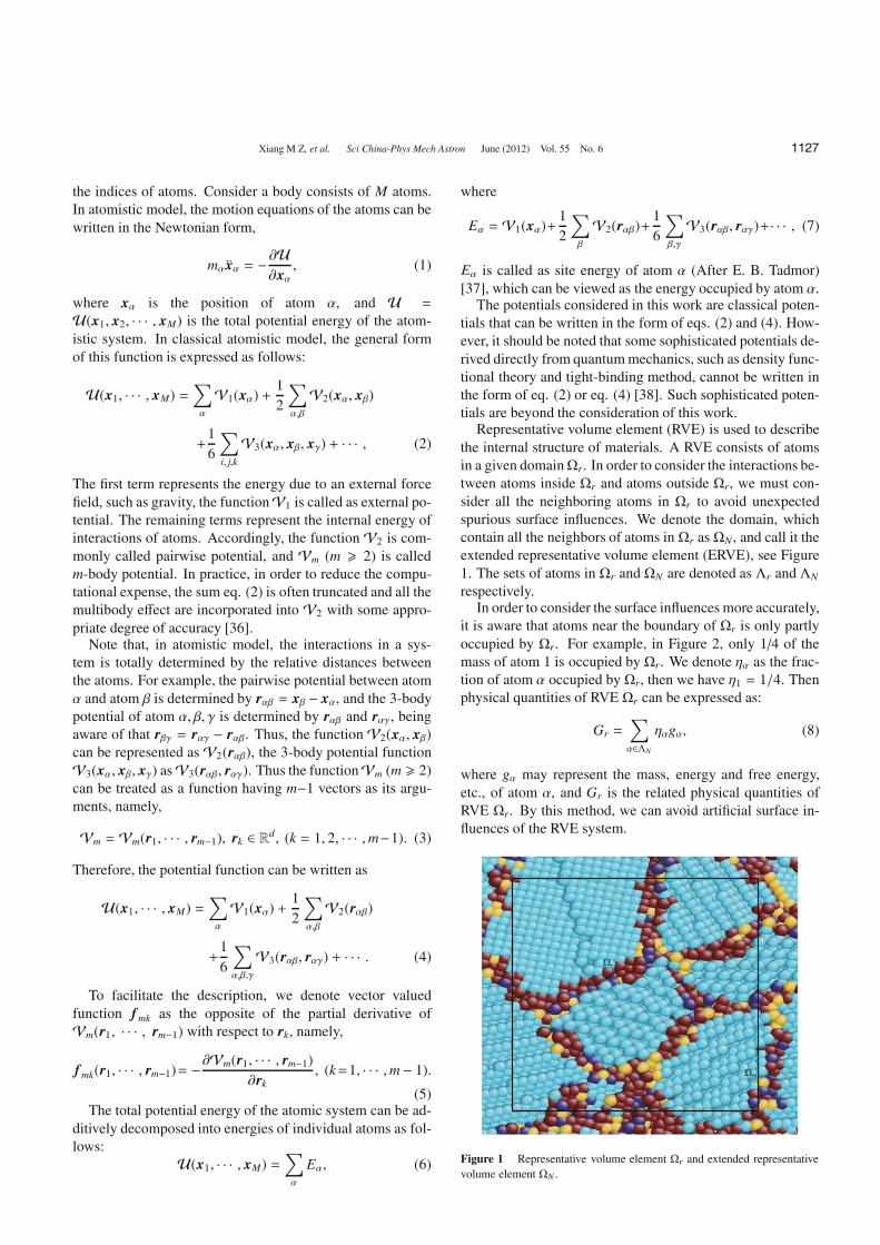
Representative volume element (RVE) is used to describethe internal structure of materials. A RVE consists of atomsin a given domainΩr. In order to consider the interactions be-tween atoms inside Ωr and atoms outside Ωr, we must con-sider all the neighboring atoms in Ωr to avoid unexpectedspurious surface influences. We denote the domain, whichcontain all the neighbors of atoms in Ωr as ΩN , and call it theextended representative volume element (ERVE), see Figure1. The sets of atoms in Ωr and ΩN are denoted as Λr and ΛN

respectively.In order to consider the surface influences more accurately,

it is aware that atoms near the boundary of Ωr is only partlyoccupied by Ωr. For example, in Figure 2, only 1/4 of themass of atom 1 is occupied by Ωr. We denote ηα as the frac-tion of atom α occupied by Ωr, then we have η1 = 1/4. Thenphysical quantities of RVE Ωr can be expressed as:

Gr =∑

α∈ΛN

ηαgα, (8)

where gα may represent the mass, energy and free energy,etc., of atom α, and Gr is the related physical quantities ofRVE Ωr. By this method, we can avoid artificial surface in-fluences of the RVE system.

Ωr

ΩN

Figure 1 Representative volume element Ωr and extended representativevolume element ΩN .


1 2

3 4

5Ωr

ΩN

Figure 2 The occupied fractions: η1 = η2 = η3 = η4 = 1/4, η5 = 1.

We should be cautious when constructing RVE systemnear surface of nanomaterials. Because of the large surface-to-volume ratios, surface effects can significantly affect themacroscopic properties of nanomaterials. When constructingsurface RVE, one should use energy minimization methodor molecular dynamics to obtain a stable atom configurationnear the surface. The problem of surface effects itself is animportant research field in nano-mechanics. We will not dis-cuss this topic in detail in the present work. More discussionof these ideas can be found in recent papers [32,33].

3 The internal energy and free energy of RVE

3.1 The changing rate of internal energy of RVE

The states of a classical atom system is represented by itsphase space coordinates (p, q), where p denotes momentumcoordinates, and q position coordinates. In order to developrelationship between atomistic model continuum model, wefirstly decompose the motion of atoms into structural defor-mation part and thermal vibration part,

q = q + q, (9)

where q denotes the positions of atoms, corresponding tostructural deformation, also the equilibrium positions of ther-mal vibrations, and q the displacements apart from structuraldeformation positions. Velocity is decomposed accordingly,

q = ˙q + ˙q. (10)

The structural deformation is relatively “slowly” changingpart of atom motions, that is, low frequency part. Thermalvibration is the high frequency part of atom motions. Thedecomposing of atom motions can be accomplished throughdifferent approaches. Zhou [21] presented a Fourier trans-form approach. As a more rough approach, the structural

deformation part can be viewed as time average of atom mo-tions:

q =1δt

t+ δt2∫

t− δt2

q(t′) dt′, (11a)

˙q=1δt

t+ δt2∫

t− δt2

q(t′) dt′. (11b)

As thermal vibration do not cause macroscopic structuraldeformation, we suppose that the average of displacements,velocities and acceleration of thermal vibrations are approxi-mately zero:

⟨ ∑

α∈Λr

ηαmα qα⟩= 0,

⟨ ∑

α∈Λr

ηαmα ˙qα⟩= 0,

⟨ ∑

α∈Λr

ηαmα ¨qα⟩= 0,

(12)

where 〈·〉 represents the average in a reasonable time intervalor statistical average. Since thermal oscillations are typicallyat frequencies in the range of 0.5–50 THz [21,39], and struc-tural deformation occurs at much lower frequencies, we rec-ommend that the time interval for average should be severalpicoseconds.

According to atomistic model, the total energy occupiedby Ωr is

Er =∑

α∈Λr

ηα

(12

mα q2α + Uα

), (13)

where Uα is potential energy of atom α. The internal energyof Ωr is

er = 〈Er〉 −∑

α∈Λr

ηα12

mα ˙q2α

=∑

α∈Λr

ηα

⟨12

mα ˙q2α

⟩+∑

α∈Λr

ηα〈Uα〉, (14)

where 〈·〉 denotes average crossing thermal vibrations. Ac-cording to eq. (14), the changing rate of the internal energyof Ωr is

er =∑

α∈Λr

ηαddt

⟨12

mα ˙q2α

⟩+∑

α∈Λr

ηα∑

β∈ΛN

∂〈Uα〉∂qβ

( ˙qβ + ˙qβ). (15)

In continuum models, the changing rate of internal energyis decomposed into two parts—work rate and heat transferrate,

er = Prinput + Qr

input, (16)

where Prinput is work rate, and Qr

input is heat transfer rate. Aswork rate is defined as inner product of force and velocity ofdeformation, thus we can write

Qrinput = er | ˙q=0

=∑

α∈Λr

ηαddt

⟨12

mα ˙q2α

⟩+∑

α∈Λr

ηα∑

β∈ΛN

∂〈Uα〉∂qβ

˙qβ(17)


and

Prinput = er − Qr

input =∑

α∈Λr

ηα∑

β∈ΛN

∂〈Uα〉∂qβ

· ˙qβ. (18)

Then from thermo-mechanics, Qrinput in the form of heat flux

can be expressed as follows:

Qrinput = −

∫

∂Ωr

h · ndS +∫

Ωr

z dX

= −∫

Ωr

div h dX +∫

Ωr

z dX,(19)

where h is heat flux, n is the unit exterior normal vector of∂Ωr, z is heat source per unit volume. Thus the changing rateof internal energy of the atom cluster in Ωr can be written as:

er =∑

α∈Λr

ηα∑

β∈ΛN

∂〈Uα〉∂qβ

· ˙qβ −∫

Ωr

div h dX +∫

Ωr

z dX. (20)

According to the second law of thermodynamics [40,41],

Sr −∫

Ωr

zT

dX +∫

Ωr

divhT

dX � 0, (21)

where Sr is entropy in Ωr. By using integration by parts,eq.(21) can be rewritten

Sr −∫

Ωr

zT

dX +∫

Ωr

div hT

dX −∫

Ωr

h · ∇TT 2

� 0. (22)

Assume temperature field in Ωr is homogeneous, then fromeq. (22), we obtain

T Sr −∫

Ωr

z dX +∫

Ωr

div h dX − 1T

∫

Ωr

h · ∇T dX � 0. (23)

By definition of Helmholtz free energy,

Ar = er − TSr , (24)

where Ar is free energy of RVE system in Ωr. Substitutingeqs. (20) and (24) into eq. (22), we obtain,

−Ar +∑

α∈Λr

ηα∑

β∈ΛN

∂〈Uα〉∂qβ

· ˙qβ − TSr − 1T

∫

Ωr

h · ∇T dX � 0.

(25)According to chain rule,

Ar =∑

β∈ΛN

∂Ar

∂qβ· ˙qβ +

∂Ar

∂TT . (26)

Takeing eq. (26) into eq. (25), the second law of thermody-namics is

(−∑

β∈ΛN

∂Ar

∂qβ+∑

α∈Λr

ηα∑

β∈ΛN

〈∂Uα〉∂qβ

)· ˙qβ

−(∂Ar

∂T+ Sr

)T − 1

T

∫

Ωr

h · ∇T dX � 0. (27)

As the above eq. (27) holds for arbitrary ( ˙q, T ), so the fol-lowing two equations is derived,

∑

α∈Λr

ηα∑

β∈ΛN

∂〈Uα〉∂qβ

=∑

β∈ΛN

∂Ar

∂qβ, (28a)

Sr = −∂Ar

∂T. (28b)

Now, by taking eq. (28a) into eq. (20), the changing rate ofinternal energy of the RVE system is obtained

er =∑

β∈ΛN

∂Ar

∂qβ· ˙qβ −

∫

Ωr

div h dX +∫

Ωr

z dX. (29)

3.2 The free energy of RVE

In order to approximately calculate the free energy, the quasi-harmonic approximation can be used. The quasiharmonic ap-proximation is quite accurate for calculating free energy ofsolids and gives results that are in good agreement with theMonte Carlo simulations [42]. The free energy is determinedby the deformation state and temperature. Here we firstlyconsider the total free energy of ERVE, which is the extendedRVE shown in Figure 1. Assume there are L atoms in ERVE,then the Hamiltonian of ERVE thermal vibration system inthe configuration defined by q can be approximated by

Hqh =

L∑

α=1

12

mα ˙q2α+U(q)+

12

L∑

α,β=1

qα ·∂U(q)∂qα∂qβ

∣∣∣∣∣∣q=q

· qβ, (30)

which can be expressed in matrix form

Hqh =12

(M12 ˙q)T(M

12 ˙q) +U(q) +

12

qTKq, (31)

where M is the mass matrix, and

K =∂U(q)∂q∂q

∣∣∣∣∣q=q

(32)

is the dynamical matrix, which is determined by the struc-ture deformation positions q and the potential functions ofthe atom system.

In following discussion, it is necessary to assert the pos-itive definiteness of the dynamical matrix K. As the freeenergy is used to determine macro constitutive relations ofmaterials, so the free energy can be computed only when theERVE system is in stable state. If it is not stable in a givenatom configuration, it must be equilibrated to stable state bymolecular dynamics or by potential energy minimization toobtain such stable atomic positions {qα}α∈ΛN , which equiva-lently ensures the positive definiteness of K.


Denote the eigenvalues of matrix M−12 KM−

12 as w2

i (i =1, · · · , 3L). Then using a normal mode transformation, theHamiltonian can be normalized to

Hqh =12

dL∑

i=1

Qi2+

12

dL∑

i=1

w2i Q2

i +U(q), (33)

where Qi (i = 1, · · · , 3L) are called normal coordinates,which are linear combination of thermal vibration coordi-nates

Qi =

dL∑

j=1

Mi jq j, (34)

whereMi j is element of the linear transformation matrixM.Then according to quantum mechanics, the free energy of

the ERVE can be approximately expressed as follows:

A(q, T ) = −kBT lnZ

= U(q, T ) + kBTdL∑

i=1

ln(2 sinh

�wi

2kBT

),

(35)

where Z denotes partition function. If semi classical approx-imation is used, then

A(q, T ) = −kBT lnZ

= U(q) − kBTdM lnkBT�+ kBT

dL∑

i=1

ln wi.(36)

The free energy of ERVE can be commonly written as:

A(q, T ) = U(q, T ) + E(q, T ) =L∑

α=1

Uα +dL∑

i=1

Ei, (37)

where Ei is the thermal vibration energy corresponding to thenormal coordinates Qi,

Ei =

⎧⎪⎪⎨⎪⎪⎩kBT ln(2 sinh �wi

2kBT ), (quantum mechanics),

kBT ln wi, (semi classical approximation).(38)

Whether quantum mechanics or semi classical approxi-mation should be used to derive Ei is dependent on eachcase. Generally speaking, in cases where temperature ismuch lower than room temperature, quantum mechanics for-mulation must be used, and formulation based on semi clas-sical approximation can be used when temperature is not toolow.

In our atomistic-continuum model, the free energy of RVEis defined in the following form

Ar =∑

α∈Λr

ηαAα. (39)

As ERVE system is inhomogeneous, the free energy of eachatom may be different. We must find a reasonable way todefine the free energyAα of a single atom α.

From eq. (37), the total free energy is composed of twoterms. First term is potential energy, second is free energy

due to thermal vibration. The first is in a form summing overall the atoms, thus the potential energy of atom α is Uα. How-ever, the second is in a form summing over all the normalcoordinates, so Ei is shown as the thermal vibration energycorresponding to normal coordinates Qi. The energy Ei maybe related to all atoms. Here, a method to define the thermalvibration energy of each atom is developed, so that the secondpart of eq. (37) can be expressed in the following form,

E =L∑

α=1

Eα, (40)

where Eα is thermal vibration energy of atom α.According to eq. (34), the elementMi j of the transforma-

tion matrixM decides the degree of correlation between Qi

and q j. We denote Gi→ j as the energy from Qi to q j, andGi→αas the energy allotted from Qi to atom α.

The approach for allotting energy Ei to atoms is notunique. However, a reasonable allotting approach should atleast satisfy the following principles:

(1) Conservation principle:

Ei =

dL∑

j=1

Gi→ j. (41)

(2) Monotony principle: If |Mi j| > |Mik |, which indicatesthat Qi depends more on q j than on qk, thus Gi→ j > Gi→k

should hold.(3) Independency principle: If |Mi j| = 0, which indicates

that Qi is independent of q j, thus Gi→ j = 0 should hold.One of the simplest approaches for allotting Ei to q j that

make the above mentioned three principles be satisfied is,

Gi→ j = ci jEi =M2

i j

dL∑k=1M2

ik

Ei. (42)

As the kth components of coordinates of atom α isqd(α−1)+k, therefore,

Gi→α =d∑

k=1

Gi→d(α−1)+k =

d∑

k=1

M2i,d(α−1)+k

dL∑k=1M2

ik

Ei, (43)

the total thermal vibration free energy of atom α,

Eα =dL∑

i=1

Gi→α

=

dL∑

i=1

d∑

k=1

M2i,d(α−1)+k

dL∑l=1M2

il

Ei.(44)

For simplicity, let

Hiα =

d∑

k=1

M2i,d(α−1)+k

dL∑l=1M2

il

. (45)


Eα can be written as

Eα =dL∑

i=1

HiαEi. (46)

The free energy of atom α is thus determined

Aα = Uα + Eα = Uα +dL∑

i=1

HiαEi. (47)

The free energy of RVE is then evaluated by eq. (39).

4 The atomistic-continuum equations forthermo-mechanical behavior

In this section, the atomistic-continuum thermo-mechanicalequations will be derived from energy analysis presented pre-viously. The Lagrangian description is used at the continuumlevel. The deformation gradient (denoted as F) is used as lo-cal strain measure and the Piola-Kirchhoff stress of the firstkind (denoted as P) is used as stress measure.

In sects. 4.1 and 4.2, the atomistic-continuum momentumand energy equations are derived in a general sense. Thenin sect. 4.3, the atomistic-continuum constitutive relationsbased the free energy expression of quasi-harmonic approxi-mation is then obtained.

4.1 The atomistic-continuum momentum equation

Atomistic model is connected to continuum model through adeformation environment assumption which has been prosedpreviously [35]. We will use similar skills to derive nonlocalthermomechanical continuum models. First of all, the defini-tion of deformation environment is given.

The deformation environment of a point X in RVE is de-fined as a tensor valued function HX,

HX(Y) = F(X + Y), ∀X + Y ∈ Ω0, (48)

where F is deformation gradient. The deformation environ-ment is based on deformation gradient. However it is dif-fers from deformation gradient in the following two aspects.Firtly, while deformation gradient is a local measure of de-formation, deformation environment is a nonlocal measuretaking the deformation states of neighbor points into consid-eration. Secondly, deformation gradient of a given point X isa tensor, but deformation of a given point X is a tensor val-ued function. By using deformation environment to describethe atom configuration corresponding to a continuum point,strain energy density (or free energy density) of that pointis a functional of the strain field, not a function of the localstrain. It is the use of this concept to connect atomistic config-uration with continuum strain field that ultimately results innonlocality of atomic interactions being built into continuumconstitutive relations. In the following of this section, the de-tails of deriving nonlocal continuum constitutive relations arepresented.

In order to derive an expression of the free energy densityof a point X in continuum sense, we assume that deforma-tion environment function of the centroid of RVE is equal tothat at point X. Then we calculate the free energy of RVE,and divide it by the volume of RVE to obtain the free energydensity expression at X,

A(X) =1VrAX

r

=1Vr

∑

α∈Λr

ηαAXα ,

(49)

whereAXα is the free energy of atom α in RVE.

Then we can calculate the total free energyA of the con-tinuum region from eq. (49), and its variation δA:

δA = 1Vr

∑

α∈Λr

ηα

1∫

0

∫

Ω0

∑

β∈ΛN

{Cαβ( ∫ 1

0F(X

+ Xα + s (X1 − Xα)) ds · (X1 − Xα), · · · ,∫ 1

0F(X + Xα + s (XL − Xα)) ds · (XL − Xα)

)

· δF(X + Xα + s′ (Xβ − Xα)) · (Xβ − Xα)

+ Bαβ( ∫ 1

0F(X + Xα + s (X1 − Xα)) ds

· (X1 − Xα), · · · ,∫ 1

0F(X + Xα + s (XL − Xα)) ds · (XL − Xα), T

)

· δF(X + Xα + s′ (Xβ − Xα)) · (Xβ − Xα)}

dXds′,(50)

where

Cαβ(r1, · · · , rL) =∂Uα(r1, · · · , rL)

∂rβ,

Bαβ(r1, · · · , rL, T ) =∂Eα(r1, · · · , rL, T )

∂rβ.

(51)

The free energy is the part of internal energy which canconvert into work. As temperature is kept constant,

δA =∫

Ω0

P : δFT dX. (52)

From eqs. (50) and (52), we can obtain the stress-strain rela-tionship as

P(X) =1Vr

∑

α∈Λr

ηα∑

β∈ΛN

∫ 1

0(Xβ − Xα)

⊗{Cαβ( ∫ 1

0F(X + (s − s′) (X1 − Xα)) ds · (X1 − Xα), · · · ,

∫ 1

0F(X + (s − s′) (XM − Xα)) ds · (XL − Xα)

)

+ Bαβ( ∫ 1

0F(X + (s − s′) (X1 − Xα)) ds · (X1 − Xα),


· · · ,∫ 1

0F(X+(s−s′) (XM−Xα)) ds·(XL−Xα), T

)}ds′. (53)

This stress-strain relationship is not point to point(X →X), but is point to region(X→ Ωr), so is nonlocal. The stressof a point is determined by the deformation environment ofthe RVE. The atomistic-continuum coupled momentum equa-tion is obtained at finite temperature by substituting (53) forP(X) in continuum momentum equation

ρ0(X)X = div P(X) + b(X). (54)

The stress-strain relationship eq. (53) is strictly nonlocal.If we approximate the deformation environment of X in thepresent model as follows:

HX(Y) = F(X + Y) ≈ F(X) ∀Y, (55)

then the resulting stress-strain relationship should be local,which is the same as that based on the Cauchy-Born rule,

P(X) =1Vr

∑

α∈Λr

ηα∑

β∈ΛN

(Xβ − Xα)

⊗ {Cαβ(F(X) · (X1 − Xα), · · · , F(X) · (XL − Xα))

+ Bαβ(F(X) · (X1 − Xα), · · · , F(X) · (XL − Xα), T )}.(56)

Further, Lagrangian elastic constants and thermal expansioncoefficients can be derived by writing the stress-strain rela-tionship in a linearized form:

P = C : (F − I) +B(T − T0), (57)

where I is unit tensor, T0 is reference temperature, and C isthe linear Lagrangian elastic constant tensor,

C =∂P∂F

∣∣∣∣∣F=I

=1Vr

∑

α∈Λr

ηα∑

β∈ΛN

∑

γ∈ΛN

(Xβ − Xα)

⊗{Cαβ(X1 − Xα, · · · , XL − Xα) ⊗ ∂

∂rγ

+ Bαβ(X1 − Xα, · · · , XL − Xα, T ) ⊗ ∂∂rγ

}⊗ (Xγ − Xα).

(58)

In eq. (58), there are tensor expressions like f ⊗ ∂∂r , in which

f is a vector valued function, with vector r as arguments. Thetensor product results in a second order tensor. If we denoteit as O, then

O = f ⊗ ∂∂r, (59)

then it can be written in component form as

Oi j =∂ f i

∂r j, ∀i, j = 1, · · · , d. (60)

The thermal expansion coefficients tensor B is derived as

B =∂P∂T

∣∣∣∣∣T=T0

=1Vr

∑

α∈Λr

ηα∑

β∈ΛN

(Xβ − Xα) ⊗ ∂B∂T

∣∣∣∣∣T=T0

. (61)

4.2 The atomistic-continuum energy equation

This subsection will focus on the energy conservation equa-tion. Firstly, the entropy density and internal energy densityis computed. The entropy density is

S (X) =1Vr

∑

α∈Λr

ηαSα( ∫ 1

0F(X + Xα + s (X1 − Xα)) ds

· (X1 − Xα), · · · ,∫ 1


),

(62)

where

Sα(r1, · · · , rL, T ) = −∂Eα(r1, · · · , rL, T )∂T

(63)

and internal energy density is

e(X) =1Vr

∑

α∈Λr

ηα

{Uα( ∫ 1

0F(X + Xα

+ s (X1 − Xα)) ds · (X1 − Xα),

· · · ,∫ 1


)

+ Eα( ∫ 1

0F(X + Xα + s (X1 − Xα)) ds · (X1 − Xα),

· · · ,∫ 1


)

+ TSα( ∫ 1

0F(X + Xα + s (X1 − Xα)) ds

· (X1 − Xα), · · · ,∫ 1


)}.

(64)

The changing rate of internal energy density can be givenas

e(X) =1Vr

∑

α∈Λr

ηα

{ ∑

β∈ΛN

[Cαβ( ∫ 1

0F(X

+ Xα + s (X1 − Xα)) ds · (X1 − Xα),

· · · ,∫ 1


)

·∫ 1

0F(X + Xα + s (Xβ − Xα)) ds · (Xβ − Xα)

+ Bαβ( ∫ 1

0F(X + Xα + s (X1 − Xα)) ds · (X1 − Xα),

· · · ,∫ 1


)

·∫ 1



+ T Dαβ( ∫ 1

0F(X + Xα + s (X1 − Xα)) ds · (X1 − Xα),

· · · ,∫ 1


)

·∫ 1


]

+ TDα( ∫ 1

0F(X + Xα + s (X1 − Xα)) ds · (X1 − Xα),

· · · ,∫ 1


)T},

(65)where,

Dαβ(r1, · · · , rL, T ) =∂Sα(r1, · · · , rL, T )

∂rβ,

Dα(r1, · · · , rL, T ) =∂Sα(r1, · · · , rL, T )

∂T.

(66)

Based on the deformation environment assumption, thechanging rate of internal energy of RVE at X is obtained,

Pinput(X) =1Vr

∑

α∈Λr

ηα∑

β∈ΛN

[Cαβ( ∫ 1

0F(X + Xα

+ s (X1 − Xα)) ds · (X1 − Xα), · · · ,∫ 1


)

·∫ 1


+ Bαβ( ∫ 1

0F(X + Xα + s (X1 − Xα)) ds

· (X1 − Xα), · · · ,∫ 1


)

·∫ 1


].

(67)

And from a continuum perspective,

e(X) = Pinput(X) − divh + z. (68)

Substituting eq. (65) and (67) into eq. (68), the atomistic-continuum coupled energy equation is obtained,

1Vr

∑

α∈Λr

ηα∑

β∈ΛN

T Dαβ( ∫ 1

0F(X + Xα

+ s (X1 − Xα)) ds · (X1 − Xα), · · · ,∫ 1


)

⊗ (Xβ − Xα) :∫ 1

0F(X + Xα + s (Xβ − Xα)) ds

+1Vr

∑

α∈Λr

ηαTDα( ∫ 1

0F(X + Xα + s (X1 − Xα)) ds

· (X1 − Xα), · · · ,∫ 1

0F(X + Xα + s (XL − Xα)) ds

·(XL − Xα), T)T = −divh + z. (69)

From the above equation, the specific heat at constant vol-ume, denoted as CV , can be defined as

CV =1Vr

∑

α∈Λr

ηαTDα( ∫ 1

0F(X + Xα

+ s (X1 − Xα)) ds · (X1 − Xα),

· · · ,∫ 1


).

(70)

This represents the heat needed for raising unit temperaturewhen deformation does not happen. In traditional continuumthermo-mechanical model, thermal stress tensor (also calledas specific heat at constant temperature by others [25]), whichrepresents the energy needed for unit deformation while tem-perature keeps at constant, is defined as

CT =∂e∂F, (71)

where F is deformation gradient. As in our model, the in-ternal energy of a point is not only dependent on the localdeformation gradient, but also on the deformation environ-ment, and thus it is a functional of the deformation gradientfield, so we do not define CT like that in eq. (71). If wedenote,

Cα,βT =1VrηαT Dαβ

( ∫ 1

0F(X + Xα

+ s (X1 − Xα)) ds · (X1 − Xα),

· · · ,∫ 1

0F(X + Xα + s (XL − Xα)) ds

·(XL − Xα))⊗ (Xβ − Xα), (72)

then the energy conservation eq. (69) can be written as

∑

α,β

Cα,βT :∫ 1

0F(X + Xα + s (Xβ − Xα)) ds +CV T

= −divh + z. (73)

Comparing with traditional energy conservation equation,

CT : F +CV T = −divh + z, (74)

it is found that Cα,βT and CT have same dimension and similarphysical meaning.


4.3 The constitutive relations under quasi-harmonic ap-proximation

In this subsection concrete constitutive relations are derivedfrom the free energy expression under quasi-harmonic ap-proximation, which is obtained in sect. 3.2.

We have denoted the thermal vibration energy correspond-ing to a normal coordinates as Ei in eq. (38). In sect. 3.2, wehave derived the thermal vibration free energy of atom α,

Eα =dL∑

i=1

HiαEi. (75)

Substituting eq. (75) into eq. (51), we obtain

Bαβ =dL∑

i=1

∂[Hiα(r1, · · · , rL)Ei(r1, · · · , rL, T )]∂rβ

. (76)

By substituting eq. (75) into eq. (63), the entropy of atom αis obtained,

Sα(r1, · · · , rL, T ) = −∂Eα(r1, · · · , rL, T )∂T

.

= −dL∑

i=1

Hiα(r1, · · · , rL)∂Ei(r1, · · · , rL, T )

∂rβ.

(77)

Taking eq. (77) into eq. (66), we obtain

Dαβ(r1, · · · , rL, T ) =∂Sα(r1, · · · , rL, T )

∂rβ

= −dL∑

i=1

[Hiα(r1, · · · , rL)∂rβ

· ∂Ei(r1, · · · , rL, T )∂rβ

+Hiα(r1, · · · , rL)∂2Ei(r1, · · · , rL, T )

∂r2β

](78)

and

Dα(r1, · · · , rL, T ) =∂Sα(r1, · · · , rL, T )

∂T

= −dL∑

i=1

Hiα(r1, · · · , rL)∂2Ei(r1, · · · , rL, T )

∂T 2. (79)

Substituting eq. (76) into eq. (53), we obtain the stress-strain relationship,

P(X) =1Vr

∑

α∈Λr

ηα∑

β∈ΛN

∫ 1

0(Xβ − Xα)

⊗{Cαβ( ∫ 1

0F(X + (s − s′) (X1 − Xα)) ds

· (X1 − Xα), · · · ,∫ 1

0F(X + (s − s′) (XM − Xα)) ds

· (XL − Xα))

+

dL∑

i=1

∂[Hiα(r1, · · · , rL)Ei(r1, · · · , rL, T )]∂rβ

}ds′.

(80)

And then the linear Lagrangian elastic tensor is

C =∂P∂F

∣∣∣∣∣F=I

=1Vr

∑

α∈Λr

ηα∑

β∈ΛN

∑

γ∈ΛN

(Xβ − Xα)

⊗{Cαβ(X1 − Xα, · · · , XL − Xα) ⊗ ∂

∂rγ

+

dL∑

i=1

∂[Hiα(r1, · · · , rL)Ei(r1, · · · , rL, T )]∂rβ

⊗ ∂∂rγ

∣∣∣∣∣(r1,··· ,rL)=(X1−Xα,··· ,XL−Xα)

}⊗ (Xγ − Xα). (81)

The thermal expansion coefficients tensor B is derived as

B =∂P∂T

∣∣∣∣∣T=T0

=1Vr

∑

α∈Λr

ηα∑

β∈ΛN

(Xβ − Xα)

⊗dL∑

i=1

Hiα(r1, · · · , rL)∂Ei(r1, · · · , rL, T )

∂T

∣∣∣∣∣T=T0

, (82)

where T0 is reference temperature.Substituting eqs. (78) and (79) into eqs. (70) and (72), we

obtain the the specific heat at constant volume

CV = − 1Vr

∑

α∈Λr

dL∑

i=1

ηαTHiα(r1, · · · , rL)

· ∂2Ei(r1, · · · , rL, T )

∂T 2

∣∣∣∣∣∣(r1,··· ,rL)=(y1α,··· ,yLα)

(83)

and specific heat at constant temperature

Cα,βT = −1VrηαT

dL∑

i=1

[Hiα(r1, · · · , rL)∂rβ

· ∂Ei(r1, · · · , rL, T )∂rβ

∣∣∣∣∣(r1,··· ,rL)=(y1α,··· ,yLα)

+Hiα(r1, · · · , rL)

× ∂2Ei(r1, · · · , rL, T )

∂r2β

∣∣∣∣∣(r1,··· ,rL)=(y1α,··· ,yLα)

]⊗ (Xβ − Xα),

(84)

where

yγα =∫ 1

0F(X + Xα + s (Xγ − Xα)) ds · (Xγ − Xα),

∀α ∈ Λr, γ = 1, · · · , L.

(85)

Thus, the atomistic-continuum thermo-mechanical consti-tutive relations have been derived on base of quasi-harmonicapproximation. Generally speaking, the analytical expres-sion of partial differentials of Hiα and Ei are complex, thusthey should be calculated numerically. But if more simpleassumption is used, such as local quasi-harmonic approxima-tion or Einstein approximation, then the expression should besimpler.


5 Multiscale simulation process and example

The atomistic-continuum thermo-mechanical conservationequations and constitutive equations are derived in the pre-vious sections. The multiscale simulation process is given asfollows:

(1) Start at t0, the initial displacement and temperaturefield is denoted as u0, T0, respectively. Construct initialERVE systems configurations according to micro structuresof the material.

(2) With un and Tn obtained. Construct initial sates ofERVE systems from the deformation and temperature fields.Equilibrate the ERVE systems by molecular dynamics simu-lations of potential energy minimizations to obtain deforma-tion part of atoms q.

(3) Use the nonlocal constitutive relations in previous sec-tions to calculate stresses and thermal capacities.

(4) Integrate momentum and energy equations by one timestep to obtain un+1 and Tn+1.

(5) n = n + 1. Go to step (2).There are two approaches for obtaining stable state of

ERVE: molecular dynamics and potential energy minimiza-tion. Potential energy minimization may be more computa-tionally effective than molecular dynamics. However molec-ular dynamics have its own advantage in that one can cal-culate the energy transformation in molecular dynamics. Insome high strain rate problems, the quantity of thermal en-ergy transformed from mechanical work is important. In thiscase, molecular dynamics simulations is recommended.

We have applied our model to a one dimensional prob-lem, in which atoms of the material interacts through a 12−6Lenard-Jones potential,

V2(r) = 4ε[(σ

r

)12 −(σ

r

)6]. (86)

In the numerical example, the nonlocality of Lenard-Jonespotential is built into continuum model.

For simplicity, the dimensionless units that are commonlyused in molecular dynamics simulations based on Lenard-Jones potential is adopted here [43]. σ and ε is chosen asunits of length and units of energy, respectively. The mass peratom m is chosen as units of mass. Units of time is

√mσ2/ε.

Units of temperature is ε/kB, where kB is the Boltzmann con-stant. Under these dimensionless units, the potential energybetween a pair of atoms with distance r is

V2(r) = 4[(1

r

)12 −(1

r

)6]. (87)

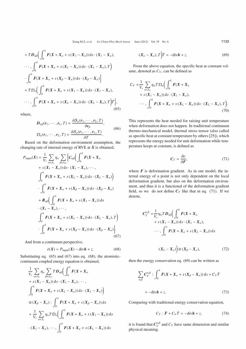
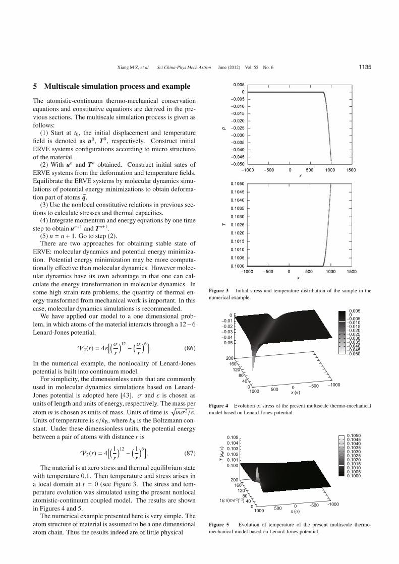
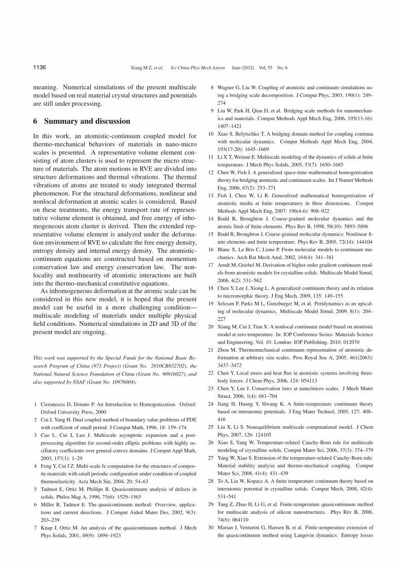
The material is at zero stress and thermal equilibrium statewith temperature 0.1. Then temperature and stress arises ina local domain at t = 0 (see Figure 3. The stress and tem-perature evolution was simulated using the present nonlocalatomistic-continuum coupled model. The results are shownin Figures 4 and 5.

The numerical example presented here is very simple. Theatom structure of material is assumed to be a one dimensionalatom chain. Thus the results indeed are of little physical

Figure 3 Initial stress and temperature distribution of the sample in thenumerical example.

0 40

80 120

160 200

−1000−500 0 500 1000

−0.05−0.04−0.03−0.02−0.01

0

x (σ)

−0.050−0.045−0.040−0.035−0.030−0.025−0.020−0.015−0.010−0.005 0 0.005

Figure 4 Evolution of stress of the present multiscale thermo-mechanicalmodel based on Lenard-Jones potential.

0 40

80 120

160 200

-1000-500 0 500 1000

0.100 0.101 0.102 0.103 0.104 0.105

0.1000 0.1005 0.1010 0.1015 0.1020 0.1025 0.1030 0.1035 0.1040 0.1045 0.1050

t ( /(m 2)1/2)ε σ

x (σ)

T (k

B/

) ε

Figure 5 Evolution of temperature of the present multiscale thermo-mechanical model based on Lenard-Jones potential.


meaning. Numerical simulations of the present multiscalemodel based on real material crystal structures and potentialsare still under processing.

6 Summary and discussion

In this work, an atomistic-continuum coupled model forthermo-mechanical behaviors of materials in nano-microscales is presented. A representative volume element con-sisting of atom clusters is used to represent the micro struc-ture of materials. The atom motions in RVE are divided intostructure deformations and thermal vibrations. The thermalvibrations of atoms are treated to study integrated thermalphenomenon. For the structural deformations, nonlinear andnonlocal deformation at atomic scales is considered. Basedon these treatments, the energy transport rate of represen-tative volume element is obtained, and free energy of inho-mogeneous atom cluster is derived. Then the extended rep-resentative volume element is analyzed under the deforma-tion environment of RVE to calculate the free energy density,entropy density and internal energy density. The atomistic-continuum equations are constructed based on momentumconservation law and energy conservation law. The non-locality and nonlinearity of atomistic interactions are builtinto the thermo-mechanical constitutive equations.

As inhomogeneous deformation at the atomic scale can beconsidered in this new model, it is hoped that the presentmodel can be useful in a more challenging condition—multiscale modeling of materials under multiple physicalfield conditions. Numerical simulations in 2D and 3D of thepresent model are ongoing.

This work was supported by the Special Funds for the National Basic Re-

search Program of China (973 Project) (Grant No. 2010CB832702), the

National Natural Science Foundation of China (Grant No. 90916027), and

also supported by NSAF (Grant No. 10976004).

1 Cioranescu D, Donato P. An Introduction to Homogenization. Oxford:

Oxford University Press, 2000

2 Cui J, Yang H. Dual coupled method of boundary value problems of PDE

with coeffcient of small period. J Comput Math, 1996, 18: 159–174

3 Cao L, Cui J, Luo J. Multiscale asymptotic expansion and a post-

processing algorithm for second-order elliptic problems with highly os-

cillatory coefficients over general convex domains. J Comput Appl Math,

2003, 157(1): 1–29

4 Feng Y, Cui J Z. Multi-scale fe computation for the structures of compos-

ite materials with small periodic configuration under condition of coupled

thermoelasticity. Acta Mech Sin, 2004, 20: 54–63

5 Tadmor E, Ortiz M, Phillips R. Quasicontinuum analysis of defects in

solids. Philos Mag A, 1996, 73(6): 1529–1563

6 Miller R, Tadmor E. The quasicontinuum method: Overview, applica-

tions and current directions. J Comput Aided Mater Des, 2002, 9(3):

203–239

7 Knap J, Ortiz M. An analysis of the quasicontinuum method. J Mech

Phys Solids, 2001, 49(9): 1899–1923

8 Wagner G, Liu W. Coupling of atomistic and continuum simulations us-

ing a bridging scale decomposition. J Comput Phys, 2003, 190(1): 249–

274

9 Liu W, Park H, Qian D, et al. Bridging scale methods for nanomechan-

ics and materials. Comput Methods Appl Mech Eng, 2006, 195(13-16):

1407–1421

10 Xiao S, Belytschko T. A bridging domain method for coupling continua

with molecular dynamics. Comput Methods Appl Mech Eng, 2004,

193(17-20): 1645–1669

11 Li X T, Weinan E. Multiscale modeling of the dynamics of solids at finite

temperature. J Mech Phys Solids, 2005, 53(7): 1650–1685

12 Chen W, Fish J. A generalized space-time mathematical homogenization

theory for bridging atomistic and continuum scales. Int J Numer Methods

Eng, 2006, 67(2): 253–271

13 Fish J, Chen W, Li R. Generalized mathematical homogenization of

atomistic media at finite temperatures in three dimensions. Comput

Methods Appl Mech Eng, 2007: 196(4-6): 908–922

14 Rudd R, Broughton J. Coarse-grained molecular dynamics and the

atomic limit of finite elements. Phys Rev B, 1998, 58(10): 5893–5896

15 Rudd R, Broughton J. Coarse-grained molecular dynamics: Nonlinear fi-

nite elements and finite temperature. Phys Rev B, 2005, 72(14): 144104

16 Blanc X, Le Bris C, Lions P. From molecular models to continuum me-

chanics. Arch Rat Mech Anal, 2002, 164(4): 341–381

17 Arndt M, Griebel M. Derivation of higher order gradient continuum mod-

els from atomistic models for crystalline solids. Multiscale Model Simul,

2006, 4(2): 531–562

18 Chen Y, Lee J, Xiong L. A generalized continuum theory and its relation

to micromorphic theory. J Eng Mech, 2009, 135: 149–155

19 Seleson P, Parks M L, Gunzburger M, et al. Peridynamics as an upscal-

ing of molecular dynamics. Multiscale Model Simul, 2009, 8(1): 204–

227

20 Xiang M, Cui J, Tian X. A nonlocal continuum model based on atomistic

model at zero temperature. In: IOP Conference Series: Materials Science

and Engineering, Vol. 10. London: IOP Publishing, 2010. 012070

21 Zhou M. Thermomechanical continuum representation of atomistic de-

formation at arbitrary size scales. Proc Royal Soc A, 2005, 461(2063):

3437–3472

22 Chen Y. Local stress and heat flux in atomistic systems involving three-

body forces. J Chem Phys, 2006, 124: 054113

23 Chen Y, Lee J. Conservation laws at nano/micro scales. J Mech Mater

Struct, 2006, 1(4): 681–704

24 Jiang H, Huang Y, Hwang K. A finite-temperature continuum theory

based on interatomic potentials. J Eng Mater Technol, 2005, 127: 408–

416

25 Liu X, Li S. Nonequilibrium multiscale computational model. J Chem

Phys, 2007, 126: 124105

26 Xiao S, Yang W. Temperature-related Cauchy-Born rule for multiscale

modeling of crystalline solids. Comput Mater Sci, 2006, 37(3): 374–379

27 Yang W, Xiao S. Extension of the temperature-related Cauchy-Born rule:

Material stability analysis and thermo-mechanical coupling. Comput

Mater Sci, 2008, 41(4): 431–439

28 To A, Liu W, Kopacz A. A finite temperature continuum theory based on

interatomic potential in crystalline solids. Comput Mech, 2008, 42(4):

531–541

29 Tang Z, Zhao H, Li G, et al. Finite-temperature quasicontinuum method

for multiscale analysis of silicon nanostructures. Phys Rev B, 2006,

74(6): 064110

30 Marian J, Venturini G, Hansen B, et al. Finite-temperature extension of

the quasicontinuum method using Langevin dynamics: Entropy losses


and analysis of errors. Model Simul Mater Sci Eng, 2010, 18: 015003

31 Wang H, Hu M, Xia M, et al. Molecular/cluster statistical thermodynam-

ics methods to simulate quasi-static deformations at finite temperature.

Int J Solids Struct, 2008, 45(13): 3918–3933

32 Yun G, Park H. A multiscale, finite deformation formulation for surface

stress effects on the coupled thermomechanical behavior of nanomateri-

als. Comput Methods Appl Mech Eng, 2008, 197(41): 3337–3350

33 Wang Z, Zhao Y. Thermo-hyperelastic models for nanostructured mate-

rials. Sci China Phys Mech Astron, 2011, 54(5): 948–956

34 Wagner G, Jones R, Templeton J, et al. An atomistic-to-continuum cou-

pling method for heat transfer in solids. Comput Methods Appl Mech

Eng, 2008, 197(41-42): 3351–3365

35 Xiang M, Cui J, Tian X, et al. Nonlocal continuum model based on

atomistic model (in Chinese). Sci China Phys Mech Astron, 2011, 41(3):

292–301

36 Liu W, Karpov E, Park H. Nano Mechanics and Materials. Chichester:

John Wiley & Sons, 2006

37 Yip S. Handbook of Materials Modeling. Berlin: Springer, 2005

38 Lakhtakia A, Thompson B, Messier R. The Handbook of Nanotechnol-

ogy. Bellingham: SPIE Press, 2004

39 Born M, Huang K. Dynamical Theory of Crystal Lattices. New York:


40 Chandler D. Introduction to Modern Statistical Mechanics. New York:


41 Weiner J. Statistical Mechanics of Elasticity. Mineola, New York: Dover

Pubns, 2002

42 Foiles S. Evaluation of harmonic methods for calculating the free energy

of defects in solids. Phys Rev B, 1994, 49(21): 14930–14938

43 Rapaport D C. The Art of Molecular Dyanmics Simulation. Cambridge:

Cambridge University Press, 2004

Date post:	25-Aug-2016
Category:	Documents
Upload:	xia
View:	212 times
Download:	0 times

Atom-continuum coupled model for thermo-mechanical behavior of materials in micro-nano scales

Documents