Atomic data and collisional-radiative modelling of neutral beams in eigenstates Oleksandr Marchuk Institute for Climate and Energy Research, Forschungszentrum Jülich GmbH, 52425, Jülich, Germany
Transcript
Atomic data and collisional-radiative modelling of neutral beams in eigenstates
Oleksandr Marchuk
Institute for Climate and Energy Research, Forschungszentrum Jülich GmbH, 52425, Jülich, Germany
Contents
• Introduction
• Linear Stark Effect for the H atom in the plasma
• Linear Zeeman-Stark Effect for the H atom in the plasma
– Impact of the Zeeman effect on the line intensities (polarization)
• Atomic data and CRM in parabolic states
• Comparison of atomic model with the ALCATOR-C Mod and JET spectra
• Conclusion and Outlook
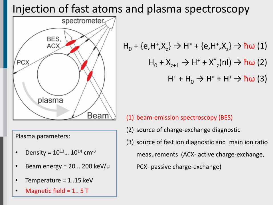
Injection of fast atoms and plasma spectroscopy
H0 + {e,H+,Xz} → H∗ + {e,H+,Xz} → ћω (1)
H0 + Xz+1 → H+ + X*z(nl) → ћω (2)
H+ + H0 → H∗ + H+ → ћω (3)
(1) beam-emission spectroscopy (BES)
(2) source of charge-exchange diagnostic
(3) source of fast ion diagnostic and main ion ratio
measurements (ACX- active charge-exchange,
PCX- passive charge-exchange)
Plasma parameters:
• Density = 1013… 1014 cm-3
• Beam energy = 20 .. 200 keV/u
• Temperature = 1..15 keV
• Magnetic field = 1.. 5 T
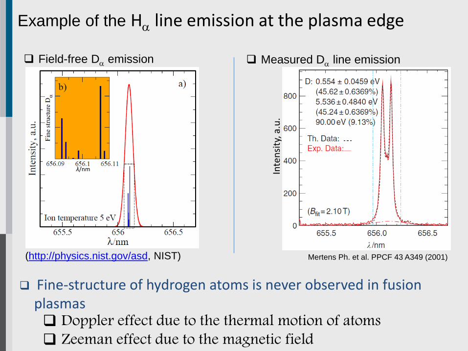
Example of the Ha line emission at the plasma edge
Field-free Da emission Measured Da line emission
Fine-structure of hydrogen atoms is never observed in fusion plasmas Doppler effect due to the thermal motion of atoms Zeeman effect due to the magnetic field
Mertens Ph. et al. PPCF 43 A349 (2001)(http://physics.nist.gov/asd, NIST)
Excited states in the active beam diagnostics• The role of the excited states in the beam penetration:
Janev R. et al. Phys. Rev. Lett. 52 534 (1984)
• The first collisional-radiative model for the beam was introduced
𝐼 𝑥 = 𝐼0 exp −𝑥
𝜆0,
𝜆0 = 1/(𝑁𝑖𝜎𝑖 𝜐) – e-folding
length,
𝑁𝑖 − is the ion density
𝜎𝑖 - is the ionization cross-section
𝜐 – is the beam velocity
x – is the distance along the beam
𝛿 = (𝜆 − 𝜆0)/𝜆• Increased (multi-step) ionization of beam atoms in the plasma → stronger attenuation
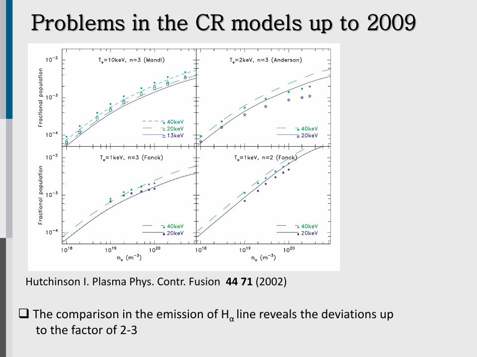
Problems in the CR models up to 2009
Hutchinson I. Plasma Phys. Contr. Fusion 44 71 (2002)
The comparison in the emission of Hα line reveals the deviations upto the factor of 2-3
Status of statistical models
Eb = 40 keV/uTe=Ti= 2 keVZeff= 1
Solid lines with points – present calculationsDashed line - Hutchinson I PPCF 44 71 (2002)
That is the first time that the population of excited states (n-states) of the beam agreewithin 20% for three different models in the density range of 1013-1014cm-3: Key component: ionization data from n=2 and n=3 states
Delabie E. et al. PPCF 52 125008 (2010)
O. Marchuk and Yu. Ralchenko, “Populations of Excited Parabolic States of Hydrogen Beam in Fusion Plasmas”, Springer-Verlagin “Atomic Processes in Basic and Applied Physics”eds by Tawara and Shevelko(2012)
(x´y´z´) is the coordinate system in therest frame of hydrogen atom
B
𝐹´ = 𝐹 +1
𝑐 𝑣 × 𝐵
𝐵´ = 𝐵 −1
𝑐 𝑣 × 𝐹
Lorentz transformation for the field:
• In the rest frame of the atom the boundelectron experiences the influence of the
crossed magnetic 𝐵´ and electric 𝐹´ fields
(cgs)
Example: B = 1 T, E = 100 keV/u → v = 4.4·108 cm/s → F = 44 kV/cm
Strong electric and magnetic field in the rest frame of the atom is experienced by thebound electron
External fields are usually considered as perturbation applied to the field-free solution
Hamiltonian is diagonal in parabolic quantum numbers
Spherical symmetry of the atom is replaced by the axial symmetry aroundthe direction of electric field.
The energy of the m –levels is not degenerated any
more in the presence of electric field (multiplet structure)
Linear Stark effect for the excited states
Fz
Parabolic quantum numbers:
n=n1+n2+|m|+1, n1, n2 ≥0 (nkm)
k=n1-n2 – electric quantum number
m – z-projection of magnetic moment
n=3
n=2𝐸 𝑛𝑘𝑚 = 3/2 · 𝐹 · 𝑛 · 𝑘 + 𝑂 𝐹2
-4 -2 4 0 2
σπ
σ0
3 2 03 1 13 0 03-1 13-2 0
2 1 02 0 1 2 -1 0
π4
n k |m|
Displacement / (3/2F)
Linear Zeeman-Stark for the excitedstates
• The angle between magnetic and electric field matters. In the case of H/D beam atomin the plasma
𝐹´ = 𝐹 +1
𝑐 𝑣 × 𝐵 (translational electric field)
• In the case of the strong field approximation (with spin) the new energy of the levels
Ω =1
2×
𝐵
𝐵0, 𝐵0= 2.35 × 10⁵ 𝑇
𝐹 =𝐸𝐿
𝐸0, 𝐸0 = 5.142 × 10¹¹ 𝑉/𝑚
Parabolic quantum numbers:
n=n1 + n2 + |m|+ 1; n1 ≥0 , n2 ≥ 0 ; k = n1 – n2 electric quantum number
Energy levels of n=2 of H atoms in the plasma
• The energy separation between different states is order of magnitude highercompared to the field free case → impact on the cross sections (LTE vs. nonLTE)
a) point-point line – Stark effect + FS ; solid line – Zeeman Stark effect + FSb) point-point line – Stark effect + FS; dashed-point line- Zeeman Stark effect ; solid line –Zeeman Stark effect + FS
k=+1
k=0
k=-1
𝛿
R. Reimer et al, RSI (to be published)
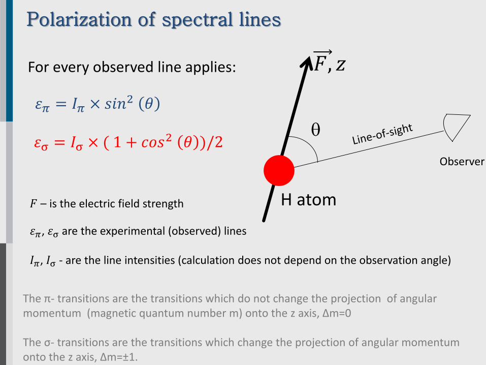
Polarization of spectral lines
휀𝜋 = 𝐼𝜋 × 𝑠𝑖𝑛2 𝜃
휀σ = 𝐼σ × ( 1 + 𝑐𝑜𝑠2 𝜃 )/2
𝐹, 𝑧
Observer
For every observed line applies:
H atom
The π- transitions are the transitions which do not change the projection of angular momentum (magnetic quantum number m) onto the z axis, ∆m=0
The σ- transitions are the transitions which change the projection of angular momentumonto the z axis, ∆m=±1.
휀𝜋, 휀σ are the experimental (observed) lines
𝐼𝜋, 𝐼σ - are the line intensities (calculation does not depend on the observation angle)
𝐹 – is the electric field strength
Comparison for the Hα multiplet betweenZeeman-Stark and Stark effect
a) thin black lines –field free case;dashed lines –Stark effect;solid lines - Stark effect + FS
b) Zeeman-Stark effect + FS
c) Change in the polarization fraction
Lines are not of „pure“ polarization
• Zeeman effect affects the polarization fraction of Stark multiplet→ impact on the pitch angle measurements
• The sum over all the and π components remains conserved
E=10 keV, B=2 T
σπ
R. Reimer et al, RSI (to be pusblished)
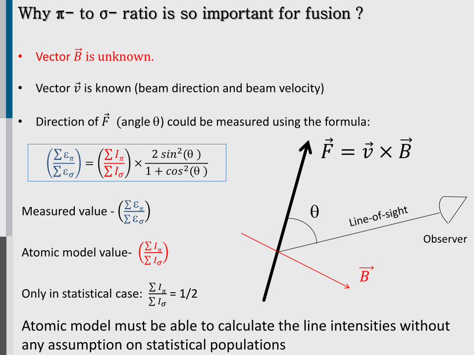
𝐹 = 𝑣 × 𝐵
Why π- to σ- ratio is so important for fusion ?
• Vector 𝐵 is unknown.
• Vector 𝑣 is known (beam direction and beam velocity)
• Direction of 𝐹 (angle ) could be measured using the formula:
Observer
𝐵
𝜋
𝜎=
𝐼𝜋 𝐼𝜎
×2 𝑠𝑖𝑛2( )
1 + 𝑐𝑜𝑠2( )
Measured value -
𝜋
𝜎
Atomic model value- 𝐼
𝜋
𝐼𝜎
Only in statistical case: 𝐼
𝜋
𝐼𝜎= 1/2
Atomic model must be able to calculate the line intensities withoutany assumption on statistical populations
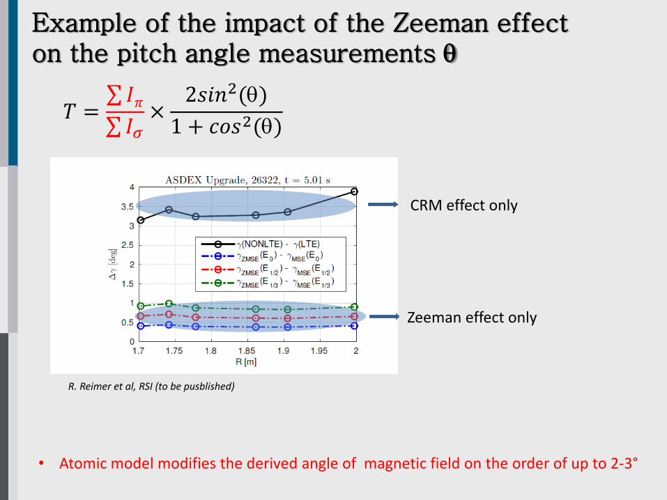
Example of the impact of the Zeeman effecton the pitch angle measurements
𝑇 = 𝐼𝜋 𝐼𝜎
×2𝑠𝑖𝑛2()
1 + 𝑐𝑜𝑠2()
• Atomic model modifies the derived angle of magnetic field on the order of up to 2-3°
Zeeman effect only
CRM effect only
R. Reimer et al, RSI (to be pusblished)
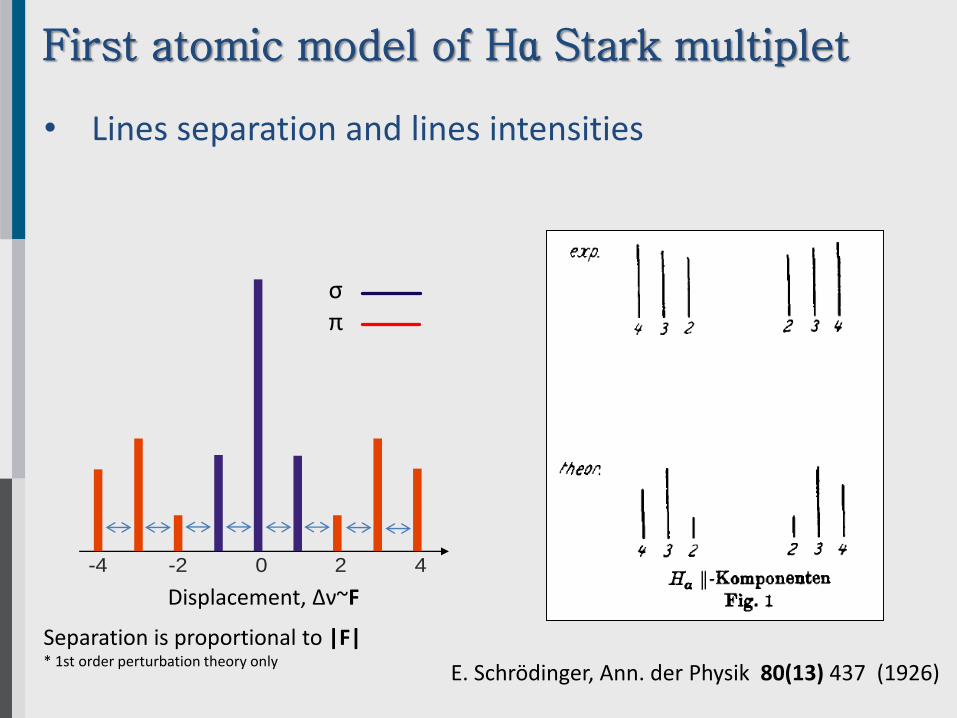
First atomic model of Hα Stark multiplet
• Lines separation and lines intensities
-4 -2 4 0 2
σπ
Displacement, Δν~F
E. Schrödinger, Ann. der Physik 80(13) 437 (1926)
Separation is proportional to |F|* 1st order perturbation theory only
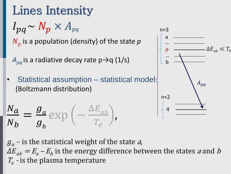
𝑔𝑎 – is the statistical weight of the state a, 𝛥𝐸𝑎𝑏 = Ea – Eb is the energy difference between the states a and bTe - is the plasma temperature
a
b
p…
…
q
𝐴𝑝𝑞
Δ𝐸𝑎𝑏 ≪ 𝑇𝑒
n=3
n=2
Beam emission spectra measured at JET Hα(n=3 → n=2)Delabie E. et al. Plasma Phys. Contr. Fusion 52 125008 (2010)
• 3 components in the beam (E/1, E/2, E/3)
• Passive light from the edge• Emission of thermal H+ and
D+
• Cold components of CII Zeeman multiplet
• Overlapped components ofStark effect spectra
𝐼 𝜃 = 𝐼𝜋sin2(𝜃) + 𝐼𝜎(1 + cos2 𝜃 )/2
• Intensity of MSE multiplet as a function of observation angle θ relative to the direction ofelectric field
• Ratios among π-(Δm=0) and σ- (Δm=±1) lines within the multiplet are well defined andshould be constant.
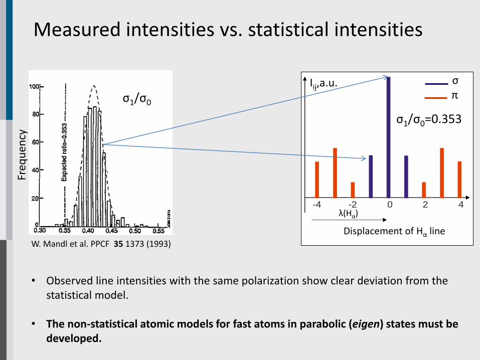
Measured intensities vs. statistical intensities
Displacement of Hα line
-4 -2 4 0 2
Iij,a.u. σπ
λ(Hα)
W. Mandl et al. PPCF 35 1373 (1993)
σ1/σ0
σ1/σ0=0.353
• Observed line intensities with the same polarization show clear deviation from thestatistical model.
• The non-statistical atomic models for fast atoms in parabolic (eigen) states must bedeveloped.
Freq
ue
ncy
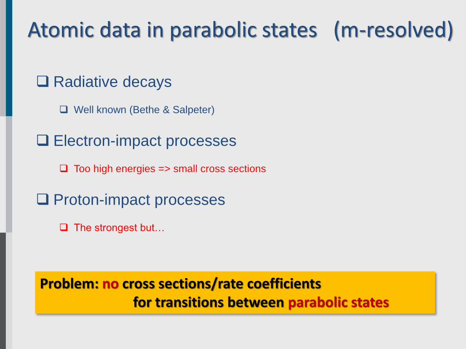
Atomic data in parabolic states (m-resolved)
Radiative decays
Well known (Bethe & Salpeter)
Electron-impact processes
Too high energies => small cross sections
Proton-impact processes
The strongest but…
Problem: no cross sections/rate coefficients for transitions between parabolic states
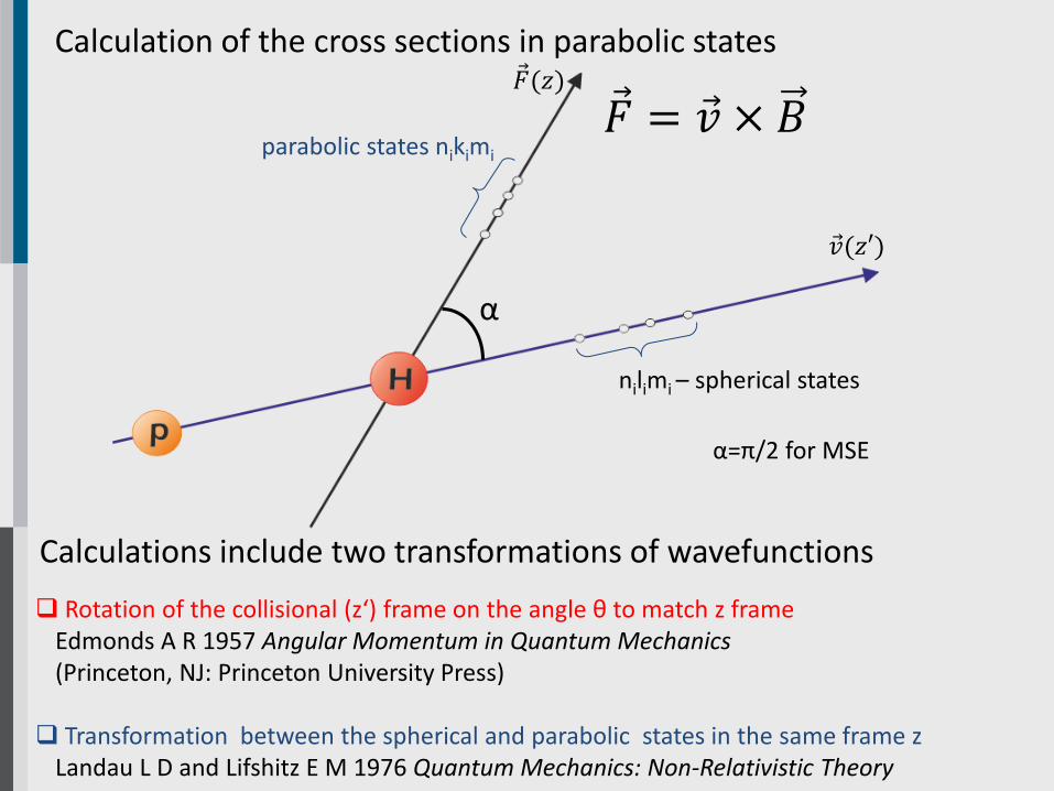
Calculation of the cross sections in parabolic states
α
parabolic states nikimi
nilimi – spherical states
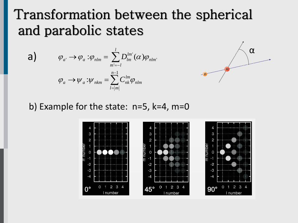
Calculations include two transformations of wavefunctions
Rotation of the collisional (z‘) frame on the angle θ to match z frameEdmonds A R 1957 Angular Momentum in Quantum Mechanics (Princeton, NJ: Princeton University Press)
Transformation between the spherical and parabolic states in the same frame zLandau L D and Lifshitz E M 1976 Quantum Mechanics: Non-Relativistic Theory
𝐹(𝑧)
𝑣(𝑧′)
α=π/2 for MSE
𝐹 = 𝑣 × 𝐵
nlm
n
ml
lm
nknkmaa
nlm
l
lm
lm
lmnlmaa
C
D
a
1
'
'
'
'
:
)(:
Transformation between the sphericaland parabolic states
a)
b) Example for the state: n=5, k=4, m=0
α
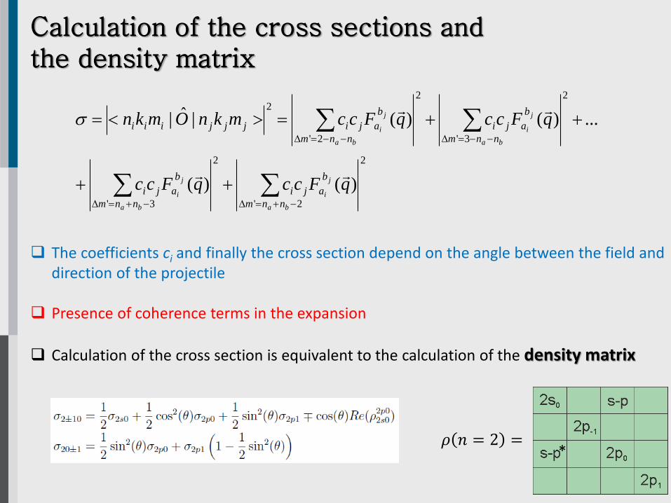
Calculation of the cross sections andthe density matrix
2
2'
2
3'
2
3'
2
2'
2
)()(
...)()(|ˆ|
ba
j
i
ba
j
i
ba
j
i
ba
j
i
nnm
b
aji
nnm
b
aji
nnm
b
aji
nnm
b
ajijjjiii
qFccqFcc
qFccqFccmknOmkn
The coefficients ci and finally the cross section depend on the angle between the field anddirection of the projectile
Presence of coherence terms in the expansion
Calculation of the cross section is equivalent to the calculation of the density matrix
𝜌 𝑛 = 2 =*
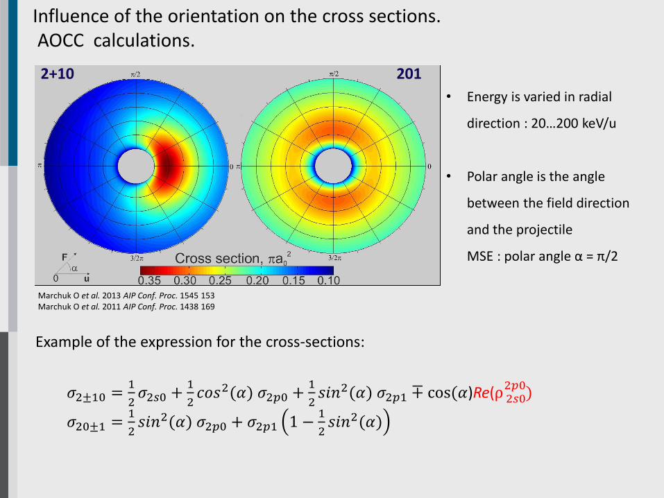
Influence of the orientation on the cross sections.AOCC calculations.
• Energy is varied in radial
direction : 20…200 keV/u
• Polar angle is the angle
between the field direction
and the projectile
MSE : polar angle α = π/2
2+10 201
Marchuk O et al. 2013 AIP Conf. Proc. 1545 153Marchuk O et al. 2011 AIP Conf. Proc. 1438 169
Example of the expression for the cross-sections:
𝜎2±10 =1
2𝜎2𝑠0 +
1
2𝑐𝑜𝑠2(𝛼) 𝜎2𝑝0 +
1
2𝑠𝑖𝑛2(𝛼) 𝜎2𝑝1 ∓ cos(𝛼)Re(ρ 2𝑠0
2𝑝0)
𝜎20±1 =1
2𝑠𝑖𝑛2(𝛼) 𝜎2𝑝0 + 𝜎2𝑝1 1 −
1
2𝑠𝑖𝑛2(𝛼)
ΔE Δn=0,F=0 << ΔE Δn=0,F≠0 << ΔE Δn>0 (*)
n1j
ΔEΔn=0
F=0 F≠0
ΔEΔn=0
n1km
n2jn2km
ΔE Δn>0 ΔE Δn>0
𝑠𝑝ℎ𝑒𝑟𝑖𝑐𝑎𝑙 𝜎 = 𝑝𝑎𝑟𝑎𝑏𝑜𝑙𝑖𝑐 𝜎 at (*)
𝑠𝑝ℎ𝑒𝑟𝑖𝑐𝑎𝑙 𝐴 = 𝑝𝑎𝑟𝑎𝑏𝑜𝑙𝑖𝑐 𝐴 at (*)
Statistical models are based on the atomic data in spherical representation The beam eigenstates are close to the parabolic ones
{φi} {ψi}
Calculation of the cross sections in parabolic states
black – AOCC calculation
blue - SAOCC Winter TG, Phys. Rev. A 2009 80 032701
green – Glauber approximation
dashed - Born approximation
orange - SAOCC Shakeshaft R Phys. Rev. A 1976 18 1930
red - EA Rodriguez VD and Miraglia JE J. Phys. B: At. Mol. Opt. Phys.
1992 25 2037
blue - AOCC calculation
green - Glauber approximation
dashed - Born approximation
orange - CC method, Schöller O et al. J. Phys B.: At. Mol. Opt. Phys. 19
2505 (1986)
red - EA Rodriguez VD and Miraglia JE J. Phys. B: At. Mol. Opt. Phys.
1992 25 2037
s-p
s-p
O. Marchuk, Yu. Ralchenko and DR Schultz Plasma Phys. Control. Fusion 54 (2012)
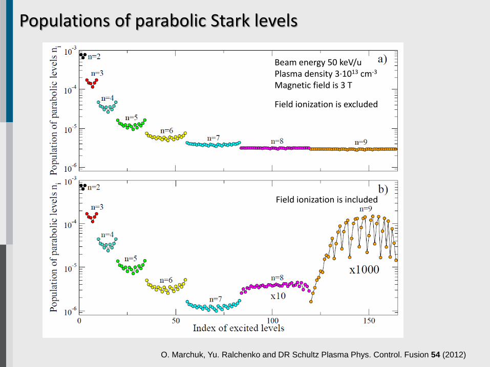
Beam energy 50 keV/uPlasma density 3·1013 cm-3
Magnetic field is 3 T
Field ionization is excluded
Populations of parabolic Stark levels
Field ionization is included
O. Marchuk, Yu. Ralchenko and DR Schultz Plasma Phys. Control. Fusion 54 (2012)
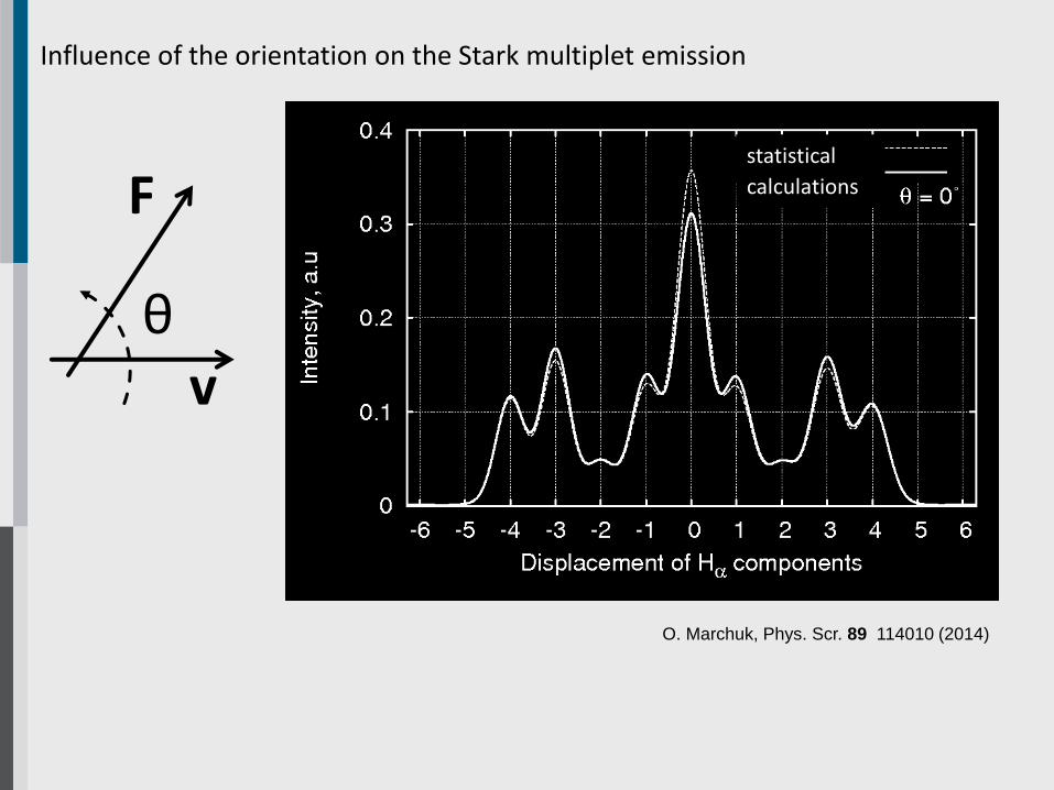
Influence of the orientation on the Stark multiplet emission
statistical
calculations
v
F
θ
O. Marchuk, Phys. Scr. 89 114010 (2014)
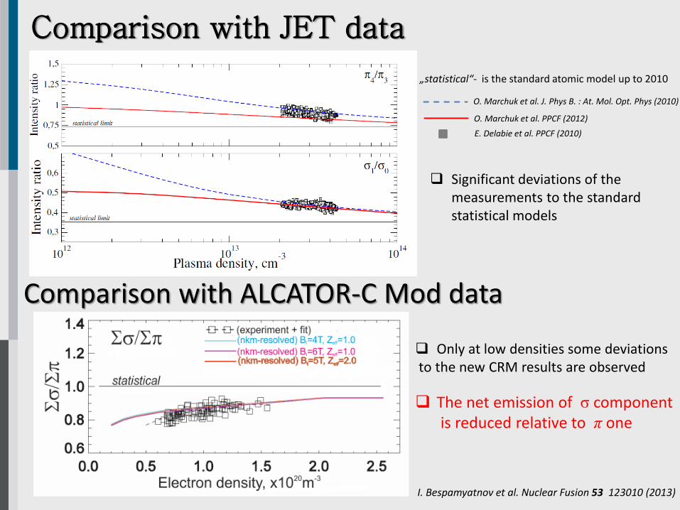
Only at low densities some deviationsto the new CRM results are observed
The net emission of σ componentis reduced relative to π one
I. Bespamyatnov et al. Nuclear Fusion 53 123010 (2013)
Comparison with JET data
Comparison with ALCATOR-C Mod data
„statistical“- is the standard atomic model up to 2010
O. Marchuk et al. J. Phys B. : At. Mol. Opt. Phys (2010)
O. Marchuk et al. PPCF (2012)
Significant deviations of themeasurements to the standardstatistical models
E. Delabie et al. PPCF (2010)
Summary
• The m-resolved model in parabolic state up to n=10 was developed..
– arbitrary orientation between the direction of the field and the atoms relative
velocity
• The collisional redistribution among the parabolic states was taken into
account in the CRM NOMAD
• The experimental data on non-statistical populations of σ- and π –
components in fusion plasma were explained …
• Impact of atomic models on the measurements of the q-profile is still


![Analysis of the X-ray and time-resolved XUV emission of ... · AVERROES/TRANSPEC NLTE collisional-radiative super-configuration code [5] are compared with experimental results. 2.](https://static.documents.pub/doc/80x56/5e6c162e43eb0a2ece4d6fff/analysis-of-the-x-ray-and-time-resolved-xuv-emission-of-averroestranspec-nlte.jpg)


