Atomic force microscopy of confined liquids using the thermal bending fluctuations of the cantilever
Fei Liu,* Sissi de Beer,† Dirk van den Ende, and Frieder MugelePhysics of Complex Fluids, MESA + Institute for Nanotechnology, University of Twente P. O. Box 217, 7500 AE Enschede, The Netherlands
(Received 16 April 2013; published 21 June 2013)
We use atomic force microscopy to measure the distance-dependent solvation forces and the dissipationacross liquid films of octamethylcyclotetrasiloxane (OMCTS) confined between a silicon tip and a highlyoriented pyrolytic graphite substrate without active excitation of the cantilever. By analyzing the thermal bendingfluctuations, we minimize possible nonlinearities of the tip-substrate interaction due to finite excitation amplitudesbecause these fluctuations are smaller than the typical 1 A, which is much smaller than the characteristic interactionlength. Moreover, we avoid the need to determine the phase lag between cantilever excitation and response, whichsuffers from complications due to hydrodynamic coupling between cantilever and fluid. Consistent results, andespecially high-quality dissipation data, are obtained by analyzing the power spectrum and the time autocorrelationof the force fluctuations. We validate our approach by determining the bulk viscosity of OMCTS using tips witha radius of approximately 1 μm at tip-substrate separations >5 nm. For sharp tips we consistently find anexponentially decaying oscillatory tip-substrate interaction stiffness as well as a clearly nonmonotonic variationof the dissipation for tip-substrate distances up to 8 and 6 nm, respectively. Both observations are in line withthe results of recent simulations which relate them to distance-dependent transitions of the molecular structurein the liquid.
Understanding the properties of nano-confined liquids is ofgreat importance in numerous research fields, like biophysics[1] and nanofluidics [2], and industrial applications, suchas friction, wear, and lubrication [3,4]. In particular, whathappens when we squeeze out a liquid between atomically flatsurfaces? At distances significantly larger than the moleculesize, the drainage process is described by the well-knownReynolds approximation [5] of the Navier-Stokes equations.However, for nano-confined liquids, where the film thicknessis comparable to the molecular size, continuum physics breaksdown and the liquid film is squeezed out layer by layer [6,7].These discrete transitions and the layering configuration arecaused by the molecular self-assembly of the liquid close tosolid walls. On confinement this gives rise to the conservativeoscillatory solvation forces [8]. These solvation forces werefirst measured in the 1980s [9] and are by now well established[10–27]. However, how molecular self-assembly affects thedynamics of the confined liquid is still heavily debated due tocontradicting experimental results.
In surface forces apparatus (SFA) experiments,confinement-induced solidification was observed whenshearing the confined liquid [28,29]. Other studies [13]reported a viscoelastic shear response akin to jamming.Measurements of the rupture process of squeezing out theliquid layer by layer could be described using a discretizedversion of the Navier-Stokes equations with a more or lessbulklike viscosity down to the last two layers [14,20]. Recentexperiments [22] and theoretical studies [30] indicate thatsome of these apparent inconsistencies can be traced down to
*[email protected]†Present address: Julich Supercomputing Centre, Wilhelm-Johnen-
Strasse, 52425 Julich, Germany.
the strong structural anisotropy in the confined liquid, whichcan lead to a highly anisotropic effective viscosity.
In more recent atomic force microscopy (AFM) experi-ments with confined liquids similar discrepancies have beenobserved. While some studies report a monotonic increase inthe viscous dissipation [10,19,26,27], others detect distance-dependent features in the dissipation [11,12,17,18,21,23–25,31,32]. All these measurements were performed usingvarious forms of dynamic AFM spectroscopy using activelydriven cantilevers. Several problems may contribute to thediscrepancies of the results reported in the literature. In liquidthe cantilever is subject to a strong mechanical couplingwith the fluid. As a consequence, the cantilever suffers fromviscous friction with the ambient fluid leading to a low overallquality factor of order unity. The damping due to the confinedliquid is only a rather small addition to the overall damping.Moreover, the coupling among the cantilever, the fluid, and thesurrounding liquid cell can give rise to additional resonances,leading to the well-known problem of a “forest of peaks”, inparticular for acoustically driven cantilevers [26,33].
Optimizations of the cantilever holder [34,35], dynamicmodels taking into account the base motion of the cantilever[26,36], as well as other (e.g., magnetic) driving schemes[37–39] help to reduce these problems, yet they do notovercome the fundamental problem that the reconstruction ofthe force is based on an inversion of the measured amplitudeand phase (or resonance frequency) and requires an accuratemodel of the cantilever dynamics, including, in particular,knowledge and calibration of the phase lag between drivingand response [40,41]. In addition, the finite drive amplitude(e.g., in excess of the molecular diameter) may “smear out”variations of interaction and dissipation forces on smallerlength scales [24].
To avoid these difficulties, we revisit the analysis of thethermal noise signal to study the conservative and dissipativeproperties of confined liquids [15,42–47]. This method, which
LIU, DE BEER, VAN DEN ENDE, AND MUGELE PHYSICAL REVIEW E 87, 062406 (2013)
has by now become a standard tool to determine the cantileverspring constant [42], minimizes the external perturbation of thesystem and it eliminates the need of a phase measurement. Weinvestigate the influence of the tip-substrate interaction on thethermal noise signal to determine both the distance-dependentinteraction stiffness due to conservative (oscillatory) tip-substrate interactions [15,43,44] and the interaction dampingdue to the local energy dissipation near the substrate. Ourapproach extends earlier studies of viscoelastic propertiesof polymeric systems [45–47] and shear forces in confinedliquids [48]. We record time series of the noise signalusing high-speed and broadband data capture and analyzeboth their power spectral density (PSD) as well as thetime autocorrelation function (ACF) [49]. Notwithstandingearlier reports of differences regarding the effect of electronicnoise [50], we find that both approaches yield consistentresults, as expected based on the Wiener-Khinchin theorem[51,52].
The conservative force and dissipation in the confined liquidare determined alternatively by fitting the obtained powerspectra and autocorrelation of the fluctuating tip displacementto a simple harmonic oscillator (SHO) model of the cantilever.The amplitude of the cantilever motion, typically 50 pm atroom temperature, is significantly smaller than that in dynamicAFM, thereby minimizing sample perturbation and ensuringthe applicability of linear response. To validate the thermalnoise method we first determine the bulk viscosity of the liquidby measuring the hydrodynamic dissipation using relativelylarge cantilever tips, with a radius of about 1 μm. This verifi-cation is referred to as the Reynolds damping measurement inthe paper. Next, we study the distance-dependent interactionforces and dissipation, using smaller tips with a radius ofabout 50 nm. Both the observed stiffness and damping oscillateas a function of the tip-substrate distance at distances below6 nm as a consequence of the layering effects, in agreementwith statistical physics [53] and molecular dynamics (MD)simulations [54].
II. METHODS
A. Materials
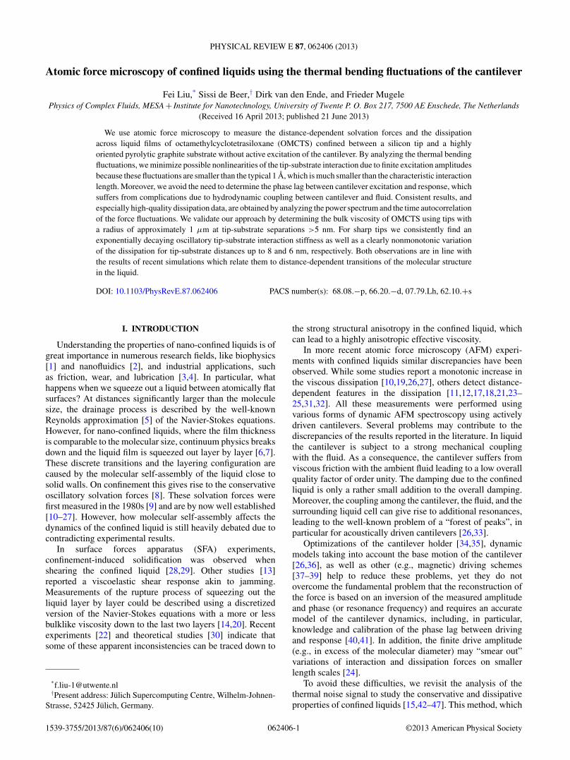
The experimental AFM setup to obtain the thermal fluc-tuations as a function of tip-substrate distance is shown inFig. 1(a). While ramping up and down the substrate close tothe tip as slow as possible, we monitor the fluctuations of the
FIG. 1. (Color online) (a) Schematic representation of the exper-imental setup. (b) Friction microscopy image of HOPG (2 × 2 nm)after Fourier filtering.
deflection signal. As a substrate we use freshly cleaved andatomic flat highly oriented pyrolytic graphite (HOPG) withan in-plane lattice constant of 0.25 nm (Mikromasch gradeZYB). For the liquid we chose octamethyl-cyclotetrasiloxane(OMCTS, as received from Fluka, purum � 99.0%) because itsmolecules have a relatively large diameter of 0.8 ∼ 0.9 nm. TheAFM device itself is a Veeco Multimode 8 with a NanoscopeV controller and Veeco EV scanner. The AFM is housed in anacoustic isolation box and operated at a constant temperatureof 300 K. For the nanoconfinement measurements, cantileverswith a sharp tip were used, from Mikromasch, which wereNSC36 aluminum coated on the back side. They have a springconstant of kc = 1 ∼ 4 N/m, as determined in air using thethermal calibration method [42], and a resonance frequency fr
in liquid between 45 and 80 kHz, as determined 8 nm awayfrom the substrate. For the Reynolds damping measurements,cantilevers with a relatively blunt silicon tip were used, fromTeam nanotech, which were LRCH coated with aluminum onthe back side. These have a kc of ∼2 N/m and a fr in liquidof ∼25 kHz. Prior to the experiments cantilevers and fluidcell are rinsed in isopropanol and ethanol, after which thecantilevers are treated for 1 min in a plasma cleaner (HarrickPlasma). After the measurements the tips are characterized byhigh-resolution scanning electron microscopy (HR-SEM ZeissLEO 1550) to estimate the tip radius and to make sure that thecantilevers were clean [55]. The sharp tips turned out to haveradii of 30 ∼ 70 nm and the blunt tips ∼900 nm.
B. Experimental procedures
As stated above, two kinds of experiments are conducted:one is done with blunt tips to validate the thermal noiseapproach by measuring the Reynolds damping and the other isdone with sharp tips to probe the dynamics in the layeredliquid. The experimental procedures are identical, but theexperimental parameters differ slightly.
The AFM is operated in force-distance mode. While thedistance between cantilever tip and substrate is varied period-ically at low speed, the deflection signal z(t) is monitored ata sampling rate of 500 kHz (i.e., over 6 times the cantilever’sfundamental eigenfrequency) using a low-pass filter with abandwidth of 200 kHz to prevent aliasing. To correct for thedrift of the piezo stage, due to thermal expansion or creep, weuse a fixed (2 ∼ 4 nm) maximum deflection of the cantilever asset point for the highest position of the stage, i.e., as retractionthreshold, after which the stage is retracted backwards overa fixed distance before the next approach is started. Fromthe variations in the approach distances we estimate that thedrift during the measurements is always less than 160 pm/s.Therefore, we choose an approach speed of 1 nm/s and a rampsize of 10 nm for the measurements with the sharp tips. Duringmeasurements with blunt tips, i.e., the Reynolds dampingmeasurements, the retraction speed, distance, and thresholdare 8 nm/s, 25 nm, and 4 nm, respectively. In both cases, theseparameters guarantee data acquisition time at acceptable drift.
In the case of sharp tips, the retraction threshold of 2 nmensures hard contact between the tip and the sample, i.e., allOMCTS will be squeezed out. This is concluded from frictionforce images recorded at the same deflection set point, whichcorresponds to a load of ∼5 nN. As shown in Fig. 1(b), these
062406-2
ATOMIC FORCE MICROSCOPY OF CONFINED LIQUIDS . . . PHYSICAL REVIEW E 87, 062406 (2013)
data reveal a hexagonal lattice (lattice constant of 0.25 nm)characteristic for HOPG.
C. Model
Although the SHO model is not fully appropriate to describethe cantilever dynamics over a wide frequency range, seeSec. V, and the Appendix for discussion of this issue, thedeviation from the full solution is only a few percentageswithin our fitting range, so this approach is more thansufficient. The SHO is driven by the Brownian force alongwith tip-substrate interactions,
m∗z + γcz + kcz = Fts + FB(t), (1)
where z is the tip position, m∗ the total effective mass(including the added mass originating from the motion ofthe surrounding liquid), γc the viscous damping around thecantilever, kc the intrinsic cantilever stiffness, Fts the distance-dependent tip-substrate interaction, and FB the random forcedue to Brownian motion, characterized by 〈FB〉 = 0 and〈FB(s)FB(s + t)〉 = 2γ kBT δ(t), where kBT is the thermalenergy and δ(t) the Dirac δ function. According to the equipar-tition theorem, the average potential energy of the cantilever,12k〈z2〉, is equal to 1
2kBT , so for a cantilever stiffness of 2 N/mthe root-mean-square displacement of the unperturbed thermalmotion is around 46 pm at room temperature. This amplitude ismuch smaller than characteristic length scale of the variationsin the tip-substrate interaction, which for OMCTS is about0.9 nm. Therefore, linearization of the tip-substrate forcearound the average tip displacement is justified, i.e., Fint =F0 − kintz − γintz, where kint is the interaction stiffness andγint is the interaction damping, and Eq. (1) can be rewritten as
m∗z + γ z + kz = FB(t), (2)
where z is now the tip displacement with respect to its averageposition at distance d, γ = γc + γint is the total dampingcoefficient, and k = kc + kint the total stiffness. Solving Eq. (2)in the frequency domain, we get
z[ω] = (k − m∗2 + jγω)−1FB[ω],
where j = √−1 is the imaginary unit. The PSD of thedisplacement z is defined as
Pzz(ω) = limts→∞
(1
tsz[ω]z[ω]∗
), (3)
where ts is the sampling time. According to the Wiener-Khinchin theorem [51,52], the PSD of the Brownian forceFB is related to its ACF as PFF (ω) = 2γ kBT . Hence, Pzz(ω)can be rewritten as
Pzz(ω) = Pw + Po[1 − (
ωωr
)2]2 + (ω
ωrQ
)2 , (4)
where Pw accounts for the instrumental (white) noise, ωr isthe resonance frequency, Q the quality factor, and Po a scalingfactor. Both Q and ωr depend on tip-substrate distance and arerelated to kint and γint by
k = kint + kc = m∗ωr2, (5a)
γ = γint + γc = m∗ωr/Q. (5b)
The effective mass m∗ is estimated by substituting the intrinsiccantilever stiffness kc and the resonance frequency ωr , asmeasured in liquid away from the substrate, where the tip-substrate interaction can be neglected, into Eq. (2). As statedbefore, the stiffness kc itself is obtained from the thermalcalibration procedure in air.
Another way to determine the interaction parameters is tomeasure the ACF of the displacement signal z(t), defined as
Rzz(t) = 1
ts
∫ ts
0z(s)z(s + t)ds. (6)
Since Rzz(t) is equal to the inverse Fourier transform of thePSD, for Q > 0.5 one can show that [56]
Rzz(t) = kBT
m∗ωr2
exp
(−ωrt
2Q
)[cos ω1t + sin ω1t√
(2Q)2 − 1
]+ R0,
(7)
where ωr = √k/m∗, ω1 = ωr
√(1 − (2Q)−2), and R0 a con-
stant to compensate for a possible background. By fittingEq. (7) to the measured ACF one again obtains values forQ and ωr .
III. DATA ANALYSIS
After we have recorded the tip displacement as a function oftime during ramping, this time sequence z(tn) is split into smalltime intervals, each of which contains 216 data points. Fromthe displacement versus time sequence in each interval thebackground, i.e., best-fitting straight line, is subtracted beforethe time sequence is transformed into a power spectral density,Eq. (3), using a standard fast-Fourier-transform algorithmto calculate z[ω]. Next, our model [Eq. (4)] is fitted to theobtained Pzz(ω), revealing values for kint(d) and γint(d), whered is the average tip-substrate distance during the consideredtime interval. Alternatively, the ACF of the time sequence iscalculated with Eq. (6) and our model function [Eq. (7)] isfitted to this correlation, again resulting in best-fit values forkint(d) and γint(d).
Although this analysis is straightforward, one has to keepin mind two aspects. First, the accuracy of the obtainedvalues for Q and ωr depends strongly on Q and the numberof data points N in the time sequence. For N = 216 andQ > 1.5 we obtain �Q/Q < 0.1 and �ωr/ωr < 0.01 duringfitting. The accuracy is further improved by averaging overseveral, typically 50, approach curves. For Q < 1 the systemis overdamped and the uncertainty in both Q and ωr stronglyincreases with decreasing Q value. In the case of sharptips in our experiments, this occurs at d < 1.5 nm. Hence,the method gives reliable results for distances larger than1.5 nm. Second, during the sampling of a time sequence thesubstrate is not stationary but travels 0.13 nm; the tip-substratedistance changes between 0.07 and 0.24 nm depending onthe tip-substrate interaction at that distance. In all cases, thisvariation is sufficiently small compared to the diameter ofthe OMCTS molecules, i.e., the length scale on which thetip-substrate interaction is expected to vary.
062406-3
LIU, DE BEER, VAN DEN ENDE, AND MUGELE PHYSICAL REVIEW E 87, 062406 (2013)
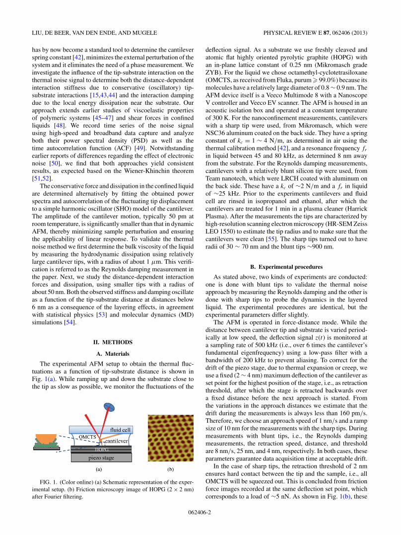
FIG. 2. (Color online) (a) Damping coefficient versus tip-substrate distance extracted from 25 approaches. Black line: averageddata, using a 25-point moving average. Red curve: best fit [Eq. (8)]to the data for damping coefficient. The inset shows the measured(smoothed) PSD (symbols) at three different distances denoted by thearrows in the main graph (solid lines are fits to our model function).(b) Inverse of Reynolds damping coefficient as a function oftip-substrate distance. Black line: averaged data, using a 25-pointmoving average. Red line: linear fit curve. The inset shows theSEM image of the tip used in the experiments (R = 900 nm,red circle). Parameter values of cantilever: kc = 1.91 ± 0.06 N/m;fr = ωr/2π = 25.2 ± 0.3 kHz in liquid at d ≈ 21 nm (m∗ = 7.61 ×10⁻¹¹ kg).
IV. RESULTS
We first discuss the validation of our method using theReynolds damping measurements with blunt tips of radiusRtip ≈ 900 nm. The inset of Fig. 2(a) gives three exemplarypower spectra with best-fit curves at various distances in-dicated by the (color matched) arrows in the main panel.The spectra are extracted from 25 approach curves, measuredconsecutively with the same tip. As the distance decreases, thepeaks in the power spectra become broader, i.e., the fitted Q
values become smaller, and the resonance shifts towards lowerfrequencies. From the fitted Q values we calculate the dampingcoefficient using Eq. (5b). The total damping increases mono-tonically with decreasing tip-substrate distance. The expectedhydrodynamic Reynolds damping due to the confined liquidunder the tip is given by
γ (d) = γc + 6πηR2
tip
d − �, (8)
where γc is the damping experienced by the cantilever beamand � is an offset to compensate for the error in zeroseparation. η is the viscosity of the liquid.
To ensure bulk behavior, we exclude data at distances lessthan 5 nm from the fit. This lower limit is obtained from theresults of measurements with a sharp tip (see below). FittingEq. (8) to our data, we find a viscosity η = 2.7 ± 0.2 mPa s,in agreement with literature data: 2.2 ∼ 2.5 mPa s [24,57].For � we obtain a value of about 0.8 nm, which indicatesthat an equivalent of one molecular layer remains rigidly stuckto one of the two the solid surfaces in qualitative agreementwith earlier SFA measurements [6,14]. To examine the qualityof the fit, the inverse of the Reynolds damping has beenplotted versus the tip-substrate distance in Fig. 2(b). The
inverse damping indeed shows a linear behavior, down to thesmallest tip-substrate distances [58]. From this observation weconclude that the choice of the lower bound of 5 nm in ouranalysis is not critical and that slip is absent in our system (asexpected for a complete wetting system).
We also validated the conservative tip-substrate forces byextracting the force gradient from the distance-dependentresonance frequency. For separations larger than 9 nm, we finda monotonically increasing attraction that can be describedby van der Waals interaction between the tip and graphitesubstrate across the liquid film (see Fig. S1 in the SupplementalMaterial [59]). At d < 6 nm, the attraction becomes repulsive,with a weak oscillatory component superimposed. Whilethe oscillation has the expected periodicity corresponding tomolecular diameter, the features are not very pronounced,presumably due to the poorly defined geometry of the largetips on small scales.
Overall, these validation measurements demonstrate thatour method does indeed yield quantitatively correct values forthe forces, including in particular dissipative forces down toa few nanometers of tip-substrate separation. They providea crucial link between well-established continuum physicsand the nanoscale behavior to be described below, which hasproven difficult to achieve in many earlier studies of confinedliquids.
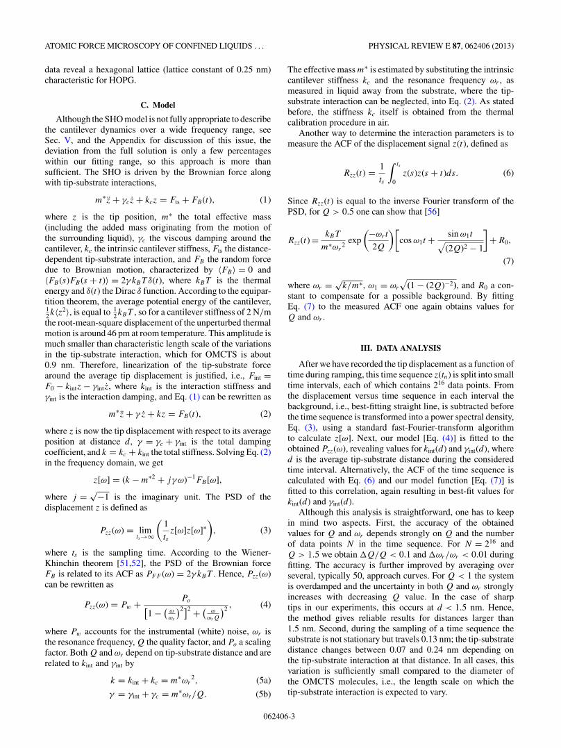
In Figs. 3–5 we present the tip-substrate interactionsmeasured with a sharp tip close to the substrate. The mainpanel of Fig. 3 shows the average deflection of the cantileverduring approach up to the retraction threshold of 2 nm. Theinsets show the measured PSDs (right) and ACFs (left) at threedifferent distances indicated by the (color-matched) arrowsin the main graph. The solid lines represent our model fits[Eqs. (4) and (7)] from which we extract the values of ωr
and Q. At distances corresponding to positive (negative) forcegradients, as denoted by an olive (blue) arrow, the resonance
FIG. 3. (Color online) Measured cantilever deflection (gray) uponapproach of the tip towards the surface at 1 nm/s (black line, averageddata, using a 216-point moving average). The inset shows the measuredautocorrelations Rzz and measured (smoothed) power spectrumdensity PSDs (symbols) at three different distances denoted by thearrows in the main graph (solid lines are fits to our model function).Data at d < 1.5 nm are shadowed, because they are not taken intoaccount in further analysis; see Figs. 4 and 5. Cantilever parameters:Rtip = 45 nm, kc = 2.71 ± 0.08 N/m; fr = 67.5 ± 0.2 kHz, andQ = 2.82 ± 0.08 at d = 8 nm (m∗ = 1.51 × 10⁻¹¹ kg).
062406-4
ATOMIC FORCE MICROSCOPY OF CONFINED LIQUIDS . . . PHYSICAL REVIEW E 87, 062406 (2013)
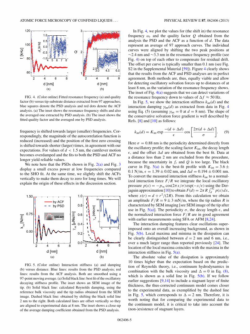
FIG. 4. (Color online) Fitted resonance frequency (a) and qualityfactor (b) versus tip-substrate distance extracted from 97 approaches;blue squares denote the PSD analysis and red dots denote the ACFanalysis. (a) The inset shows the resonance frequency shifts and alsothe averaged one extracted by PSD analysis. (b) The inset shows thefitted quality factor and the averaged one by PSD analysis.
frequency is shifted towards larger (smaller) frequencies. Cor-respondingly, the magnitude of the autocorrelation function isreduced (increased) and the position of the first zero crossingis shifted towards shorter (larger) times, in agreement with ourexpectations. For values of d < 1.5 nm, the cantilever motionbecomes overdamped and the fits to both the PSD and ACF nolonger yield reliable values.
We note here that the PSDs shown in Fig. 2(a) and Fig. 3display a small excess power at low frequencies comparedto the SHO fit. At the same time, we slightly shift the ACFsvertically to make them decay to zero for long times. We willexplain the origin of these effects in the discussion section.
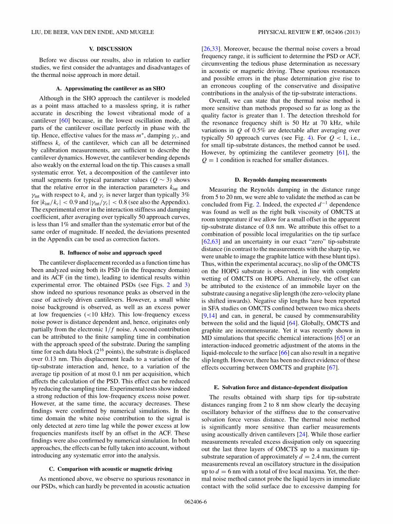
FIG. 5. (Color online) Interaction stiffness (a) and damping(b) versus distance. Blue lines: results from the PSD analysis; redlines: results from the ACF analysis. Both are smoothed using a97-point moving average. (a) Solid black line: best fit of the oscillatorydecaying stiffness profile. The inset shows an SEM image of thetip. (b) Solid black line: calculated Reynolds damping, using thereference bulk viscosity and the tip radius obtained from the SEMimage. Dashed black line: obtained by shifting the black solid line2 nm to the right. Both calculated lines are offset vertically so theyare aligned to experimetnal data at 8 nm. The inset shows a close-upof the average damping coefficient obtained from the PSD analysis.
In Fig. 4, we plot the values for (the shift in) the resonancefrequency ωr and the quality factor Q obtained from theanalysis the PSD and the ACF as a function of d. The datarepresent an average of 97 approach curves. The individualcurves were aligned by shifting the two peak positions at∼2.4 nm and ∼3.3 nm in the resonance frequency profile (seeFig. 4) on top of each other to compensate for residual drift.The offset per curve is typically smaller than 0.1 nm (see Fig.S2 in the Supplemental Material [59]). Figure 4 clearly showsthat the results from the ACF and PSD analyses are in perfectagreement. Both methods are, thus, equally viable and allowfor detecting oscillatory solvation forces up to distances of atleast 8 nm, as the variation of the resonance frequency shows.The inset of Fig. 4(a) suggests that we can detect variations ofthe resonance frequency down to values of �f ≈ 50 Hz.
In Fig. 5, we show the interaction stiffness kint(d) and theinteraction damping γint(d) as extracted from data in Fig. 4using Eq. (5) (assuming γint = 0 at d = 8 nm). The shape ofthe conservative solvation force gradient is well described byRefs. [8] and [10] as follows:
kint(d) = Kint exp−(d + �d)
εcos
[2π (d + �d)
σ
]. (9)
Here σ = 0.88 nm is the periodicity determined directly fromthe oscillatory profile; the scaling factor Kint, the decay lengthε, and the offset �d are obtained from the best fit. Data ata distance less than 2 nm are excluded from the procedure,because the uncertainty in fr and Q is too large. The blackcurve in Fig. 5(a) is the best-fit profile with Kint = 3.6 ±0.1 N/m, ε = 1.39 ± 0.02 nm, and �d = 0.194 ± 0.001 nm.To convert the measured interaction stiffness kint to a normal-ized interaction force F/R we integrate the local oscillatorypressure p(x) = −p∞ cos(2πx/σ ) exp(−x/ε) using the Der-jaguin approximation [10] to obtain F (d) = 2πR
∫ ∞d
p(x) dx,where x(r) = d + r2/(2R). From this calculation we obtainan amplitude F/R = 9 ± 3 mN/m, where the tip radius R ischaracterized by SEM imaging [see SEM image of the tip afteruse in Fig. 5(a)]. The periodicity σ , the decay length ε, andthe normalized interaction force F/R are in good agreementwith earlier measurements using SFA or AFM [8,24].
The interaction damping features clear oscillations super-imposed onto an overall increasing background, as shown inFig. 5(b). Local maxima and minima in the dissipation canbe clearly distinguished between d = 2 nm and 6 nm, i.e.,over a much larger range than reported previously [24]. Thelocation of the local maxima coincides with the maxima in theinteraction stiffness in Fig. 5(a).
The absolute value of the dissipation is approximately10 times higher than the expectation based on the predic-tion of Reynolds theory, i.e., continuum hydrodynamics incombination with the bulk viscosity and � = 0 in Eq. (8),which is shown as a solid line in Fig. 5(b). If we followearlier suggestions [9,14] to include a stagnant layer of finitethickness, the thus-corrected continuum model comes closerto the experimental data, as exemplified by the dashed linein Fig. 5, which corresponds to � = 2 nm. Therefore, it isworth noting that for comparing the experimental data tothe continuum model, it is critical to take into account the(non-)existence of stagnant layers.
062406-5
LIU, DE BEER, VAN DEN ENDE, AND MUGELE PHYSICAL REVIEW E 87, 062406 (2013)
V. DISCUSSION
Before we discuss our results, also in relation to earlierstudies, we first consider the advantages and disadvantages ofthe thermal noise approach in more detail.
A. Approximating the cantilever as an SHO
Although in the SHO approach the cantilever is modeledas a point mass attached to a massless spring, it is ratheraccurate in describing the lowest vibrational mode of acantilever [60] because, in the lowest oscillation mode, allparts of the cantilever oscillate perfectly in phase with thetip. Hence, effective values for the mass m∗, damping γc, andstiffness kc of the cantilever, which can all be determinedby calibration measurements, are sufficient to describe thecantilever dynamics. However, the cantilever bending dependsalso weakly on the external load on the tip. This causes a smallsystematic error. Yet, a decomposition of the cantilever intosmall segments for typical parameter values (Q ∼ 3) showsthat the relative error in the interaction parameters kint andγint with respect to kc and γc is never larger than typically 3%for |kint/kc| < 0.9 and |γint/γc| < 0.8 (see also the Appendix).The experimental error in the interaction stiffness and dampingcoefficient, after averaging over typically 50 approach curves,is less than 1% and smaller than the systematic error but of thesame order of magnitude. If needed, the deviations presentedin the Appendix can be used as correction factors.
B. Influence of noise and approach speed
The cantilever displacement recorded as a function time hasbeen analyzed using both its PSD (in the frequency domain)and its ACF (in the time), leading to identical results withinexperimental error. The obtained PSDs (see Figs. 2 and 3)show indeed no spurious resonance peaks as observed in thecase of actively driven cantilevers. However, a small whitenoise background is observed, as well as an excess powerat low frequencies (<10 kHz). This low-frequency excessnoise power is distance dependent and, hence, originates onlypartially from the electronic 1/f noise. A second contributioncan be attributed to the finite sampling time in combinationwith the approach speed of the substrate. During the samplingtime for each data block (216 points), the substrate is displacedover 0.13 nm. This displacement leads to a variation of thetip-substrate interaction and, hence, to a variation of theaverage tip position of at most 0.1 nm per acquisition, whichaffects the calculation of the PSD. This effect can be reducedby reducing the sampling time. Experimental tests show indeeda strong reduction of this low-frequency excess noise power.However, at the same time, the accuracy decreases. Thesefindings were confirmed by numerical simulations. In thetime domain the white noise contribution to the signal isonly detected at zero time lag while the power excess at lowfrequencies manifests itself by an offset in the ACF. Thesefindings were also confirmed by numerical simulation. In bothapproaches, the effects can be fully taken into account, withoutintroducing any systematic error into the analysis.
C. Comparison with acoustic or magnetic driving
As mentioned above, we observe no spurious resonance inour PSDs, which can hardly be prevented in acoustic actuation
[26,33]. Moreover, because the thermal noise covers a broadfrequency range, it is sufficient to determine the PSD or ACF,circumventing the tedious phase determination as necessaryin acoustic or magnetic driving. These spurious resonancesand possible errors in the phase determination give rise toan erroneous coupling of the conservative and dissipativecontributions in the analysis of the tip-substrate interactions.
Overall, we can state that the thermal noise method ismore sensitive than methods proposed so far as long as thequality factor is greater than 1. The detection threshold forthe resonance frequency shift is 50 Hz at 70 kHz, whilevariations in Q of 0.5% are detectable after averaging overtypically 50 approach curves (see Fig. 4). For Q < 1, i.e.,for small tip-substrate distances, the method cannot be used.However, by optimizing the cantilever geometry [61], theQ = 1 condition is reached for smaller distances.
D. Reynolds damping measurements
Measuring the Reynolds damping in the distance rangefrom 5 to 20 nm, we were able to validate the method as can beconcluded from Fig. 2. Indeed, the expected d−1 dependencewas found as well as the right bulk viscosity of OMCTS atroom temperature if we allow for a small offset in the apparenttip-substrate distance of 0.8 nm. We attribute this offset to acombination of possible local irregularities on the tip surface[62,63] and an uncertainty in our exact “zero” tip-substratedistance (in contrast to the measurements with the sharp tip, wewere unable to image the graphite lattice with these blunt tips).Thus, within the experimental accuracy, no slip of the OMCTSon the HOPG substrate is observed, in line with completewetting of OMCTS on HOPG. Alternatively, the offset canbe attributed to the existence of an immobile layer on thesubstrate causing a negative slip length (the zero-velocity planeis shifted inwards). Negative slip lengths have been reportedin SFA studies on OMCTS confined between two mica sheets[9,14] and can, in general, be caused by commensurabilitybetween the solid and the liquid [64]. Globally, OMCTS andgraphite are incommensurate. Yet it was recently shown inMD simulations that specific chemical interactions [65] or aninteraction-induced geometric adjustment of the atoms in theliquid-molecule to the surface [66] can also result in a negativeslip length. However, there has been no direct evidence of theseeffects occurring between OMCTS and graphite [67].
E. Solvation force and distance-dependent dissipation
The results obtained with sharp tips for tip-substratedistances ranging from 2 to 8 nm show clearly the decayingoscillatory behavior of the stiffness due to the conservativesolvation force versus distance. The thermal noise methodis significantly more sensitive than earlier measurementsusing acoustically driven cantilevers [24]. While those earliermeasurements revealed excess dissipation only on squeezingout the last three layers of OMCTS up to a maximum tip-substrate separation of approximately d = 2.4 nm, the currentmeasurements reveal an oscillatory structure in the dissipationup to d = 6 nm with a total of five local maxima. Yet, the ther-mal noise method cannot probe the liquid layers in immediatecontact with the solid surface due to excessive damping for
062406-6
ATOMIC FORCE MICROSCOPY OF CONFINED LIQUIDS . . . PHYSICAL REVIEW E 87, 062406 (2013)
d < 1.5 nm. According to Fig. 3, this implies that the localmaxima in the dissipation shown in Fig. 5(b) correspond tofilm thicknesses of three to seven molecular layers. The localmaximum at the smallest tip-substrate separation shown inFig. 5(b) (at d ≈ 2.2 nm) thus corresponds to the peak at thelargest tip-substrate separation in Refs. [24,54] at d ≈ 2.4 nm.(The absolute zero of the tip-substrate separation in Ref. [24] isoff by approximately 0.6 nm.) This assignment is corroboratedby the absolute value of γint, which is approximately 10−6 Ns/min both experiments. Comparing the sensitivity of the twoexperiments reveals a gain of approximately one order ofmagnitude in the present experiments.
The MD simulations reported in Ref. [54] suggest thatthe sharp excess dissipation on squeezing out the layersin immediate contact with the solid walls is related toconfinement-induced transitions between very well ordered(solidlike) films for film thicknesses of one, two, and perhapsthree molecular layers and rather disordered configurationsfor intermediate half-integer numbers of molecular layers.Whether that scenario also extends to the much larger tip-substrate separations studied here is not clear. At largerseparations, thermal fluctuations as well as the tip geometryon a larger scale may lead to increased disorder [68–70] and,thus, prevent the crystalline arrangement found at smallerseparations.
VI. CONCLUSION
In summary, we measured the distance-dependent solvationforces and the dissipation of OMCTS in the confinementbetween a silicon tip and an HOPG substrate using atomicforce microscopy. To obtain reliable results for the distance-dependent dissipation in the confinement, we employ thethermal noise approach, which provides a resolution ofapproximately 50 Hz in frequency shift and 10 nNs/m indamping coefficient as long as the quality factor is larger thanunity, which is the case for tip-substrate distances larger than2 nm in the present experiments. To validate the method thedistance-dependent Reynolds damping and bulk viscosity ofOMCTS were successfully measured. Close to the substratewe were able to measure the interaction stiffness due to thesolvation forces in agreement with earlier findings, whilethe damping also showed pronounced oscillations instead ofmonotonic behavior as a function of tip-substrate distance.From a technical perspective, we presented a method toperform small amplitude force microscopy without relyingon a perfect spectral response, in both amplitude and phase, tothe external actuation of the cantilever, just by analyzing thethermal noise of the cantilever, which also guarantees smallamplitudes of typically 50 pm. Moreover, it was shown thatthe thermal noise can be evaluated equally well with the powerspectral density as with the autocorrelation function.
ACKNOWLEDGMENTS
This work has been supported by the Foundation forFundamental Research of Matter (FOM), which is financiallysupported by the Netherlands Organization for ScientificResearch (NWO).
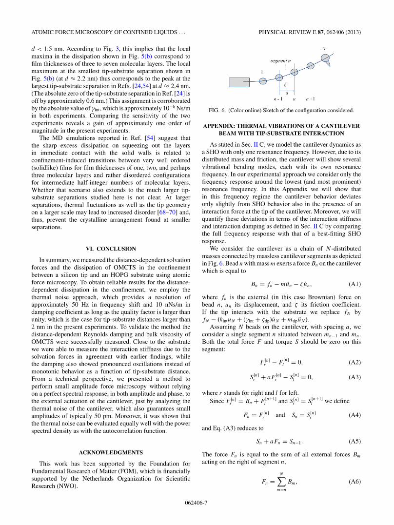
FIG. 6. (Color online) Sketch of the configuration considered.
APPENDIX: THERMAL VIBRATIONS OF A CANTILEVERBEAM WITH TIP-SUBSTRATE INTERACTION
As stated in Sec. II C, we model the cantilever dynamics asa SHO with only one resonance frequency. However, due to itsdistributed mass and friction, the cantilever will show severalvibrational bending modes, each with its own resonancefrequency. In our experimental approach we consider only thefrequency response around the lowest (and most prominent)resonance frequency. In this Appendix we will show thatin this frequency regime the cantilever behavior deviatesonly slightly from SHO behavior also in the presence of aninteraction force at the tip of the cantilever. Moreover, we willquantify these deviations in terms of the interaction stiffnessand interaction damping as defined in Sec. II C by comparingthe full frequency response with that of a best-fitting SHOresponse.
We consider the cantilever as a chain of N -distributedmasses connected by massless cantilever segments as depictedin Fig. 6. Bead n with mass m exerts a force Bn on the cantileverwhich is equal to
Bn = fn − mun − ζ un, (A1)
where fn is the external (in this case Brownian) force onbead n, un its displacement, and ζ its friction coefficient.If the tip interacts with the substrate we replace fN byfN − (kintuN + (γint + ζtip)uN + mtipuN ).
Assuming N beads on the cantilever, with spacing a, weconsider a single segment n situated between mn−1 and mn.Both the total force F and torque S should be zero on thissegment:
F [n]r − F
[n]l = 0, (A2)
S[n]r + aF [n]
r − S[n]l = 0, (A3)
where r stands for right and l for left.Since F [n]
r = Bn + F[n+1]l and S[n]
r = S[n+1]l we define
Fn = F [n]r and Sn = S[n]
r (A4)
and Eq. (A3) reduces to
Sn + aFn = Sn−1. (A5)
The force Fn is equal to the sum of all external forces Bm
acting on the right of segment n,
Fn =N∑
m=n
Bm, (A6)
062406-7
LIU, DE BEER, VAN DEN ENDE, AND MUGELE PHYSICAL REVIEW E 87, 062406 (2013)
while the torque Sn is equal to the sum of all external moments(m − n)aBm acting on the right of segment n,
Sn = a
N∑m=n
(m − n)Bm. (A7)
Solving the force and torque balance on segment n, oneobtains relations for the displacement u and the slope a du/dx
of mass n and n − 1 as follows:
un−1 = un − u′n + Sn/a
2κ+ Fn
6κ, (A8)
u′n−1 = u′
n − Sn/a
κ− Fn
2κ, (A9)
Sn−1 = Sn + aFn, (A10)
Fn−1 = Fn + Bn−1, (A11)
where κ = EI/a3 and Bn = fn − qun with q(ω) = −mω2 +jζω. With Eqs. (A8)–(A11) we can calculate all un and u′
n
values in the frequency domain starting from a guess foruN and u′
N and we will end up with the following linearrelations:
u0 = A0 uN + A1 u′N +
N∑n=1
αnfn, (A12)
u′0 = A2 uN + A3 u′
N +N∑
n=1
βnfn. (A13)
By inversion of the last two equations we can express uN andu′
N in u0, u′0 and the forces fn accordingly:
uN = A3
[A]u0 − A1
[A]u′
0 +N∑
n=1
Gn fn, Gn = βnA1 − αnA3
[A],
(A14)
u′N = A0
[A]u′
0 − A2
[A]u0 +
N∑n=1
Hn fn, Hn = αnA2 − βnA0
[A],
(A15)
with [A] = A0A3 − A1A2. The coefficients αn, βn, and An canbe calculated by evaluating Eqs. (A8)–(A11) while setting oneof the values (uN,u′
N,f1,f2, . . . ,fN ) equal to 1 and keeping allthe other values 0. Since we consider the noise response, weset both u0 and u′
0 to zero for all frequencies. Because the PSDof the Brownian forces is constant, i.e., Pf (ω) = 2ζkBT , thepower spectral density Ps(ω) of the signal u′
N (ω)/a is givenby (no interaction on the tip)
Ps(ω) = 1
a2
N∑n=1
|Hn(ω)|2 Pfn(ω)
= 2kBT
L2N2
N∑n=1
ζn |Hn(ω)|2 . (A16)
Taking into account the interaction force (and additionaltip mass) on the tip in the expression for fN , we replace it
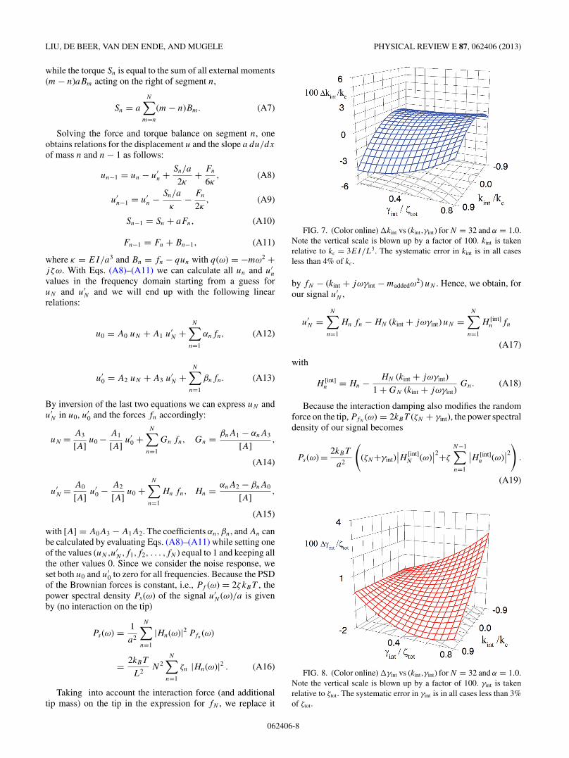
FIG. 7. (Color online) �kint vs (kint,γint) for N = 32 and α = 1.0.Note the vertical scale is blown up by a factor of 100. kint is takenrelative to kc = 3EI/L3. The systematic error in kint is in all casesless than 4% of kc.
by fN − (kint + jωγint − maddedω2) uN . Hence, we obtain, for
our signal u′N ,
u′N =
N∑n=1
Hn fn − HN (kint + jωγint) uN =N∑
n=1
H [int]n fn
(A17)
with
H [int]n = Hn − HN (kint + jωγint)
1 + GN (kint + jωγint)Gn. (A18)
Because the interaction damping also modifies the randomforce on the tip, PfN
(ω) = 2kBT (ζN + γint), the power spectraldensity of our signal becomes
Ps(ω) = 2kBT
a2
((ζN+γint)
∣∣H [int]N (ω)
∣∣2+ζ
N−1∑n=1
∣∣H [int]n (ω)
∣∣2
).
(A19)
FIG. 8. (Color online) �γint vs (kint,γint) for N = 32 and α = 1.0.Note the vertical scale is blown up by a factor of 100. γint is takenrelative to ζtot. The systematic error in γint is in all cases less than 3%of ζtot.
062406-8
ATOMIC FORCE MICROSCOPY OF CONFINED LIQUIDS . . . PHYSICAL REVIEW E 87, 062406 (2013)
To evaluate Eq. (A18) and (A19) numerically, we de-fine a reference frequency ω# = √
kc/mtot, where kc =3EI/L3. We then get, with ν = ω/ω#, for the relevantvariables,
q = −mω2#ν
2 + jζω#, (A20)
m = α mtot/N, (A21)
mN = (1 − α + α/N )mtot, (A22)
ζ = α ζtot/N, (A23)
ζN = (1 − α + α/N )ζtot, (A24)
where (1 − α)mtot is the mass of the tip. With Q−1 =ζtot/
√mtotkc we arrive at
q = αkc
N(−ν2 + jν/Q), (A25)
qN =(
α
N+ 1 − α
)kc(−ν2 + jν/Q), (A26)
and
Ps(ν) = 2kBT
L2N
{α ζtot
N∑n=1
∣∣H [int]n
∣∣2 + ((1 − α)Nζtot
+ γint)∣∣H [int]
N
∣∣2}, (A27)
where H [int]n is a function of the complex quantity [kint +
jQ−1(kc/ζtot) γint ν]; see Eq. (A18). We evaluated Eq. (A27)numerically, varying kint/kc and γint/ζtot, and fitted the ob-tained Ps(ν) curves to the SHO model. This resulted in goodfits with a low χ2 per data point. From these fits the values forkint/kc and γint/ζtot were recalculated and compared with theiroriginal values. The systematic errors �kint = kfit
int − kint and�γint = γ fit
int − γint have been plotted in Figs. 7 and 8, wherekint has been scaled on kc and γint on ζtot.
[1] L. Bocquet and E. Charlaix, Chem. Soc. Rev. 39, 1073 (2010).[2] J. C. T. Eijkel and A. van den Berg, Microfluid. Nanofluid. 1,
249 (2005).[3] B. N. J. Persson and F. Mugele, J. Phys.: Condens. Matter 16,
R295 (2004).[4] M. H. Muser, M. Urbakh, and M. O. Robbins, Adv. Chem. Phys.
126, 187 (2003).[5] O. Reynolds, Phil. Trans. R. Soc. London 177, 157 (1886).[6] D. Chan and R. Horn, J. Chem. Phys. 83, 5311 (1985).[7] F. Mugele and M. Salmeron, Phys. Rev. Lett. 84, 5796
(2000).[8] J. Israelachvili, Intermolecular and Surface Forces, 2nd ed.
(Academic Press, London, 1991).[9] R. G. Horn and J. N. Israelachvili, Chem. Phys. Lett. 71, 192
(1980).[10] S. J. O’Shea and M. E. Welland, Langmuir 14, 4186 (1998).[11] M. Antognozzi, A. D. L. Humphris, and M. J. Miles, Appl. Phys.
Lett. 78, 300 (2001).[12] M. Kageshima, H. Jensenius, M. Dienwiebel, Y. Nakayama,
H. Tokumoto, S. P. Jarvis, and T. H. Oosterkamp, Appl. Surf.Sci. 188, 440 (2002).
[13] Y. Zhu and S. Granick, Langmuir 19, 8148 (2003).[14] T. Becker and F. Mugele, Phys. Rev. Lett. 91, 166104 (2003).[15] P. D. Ashby and C. M. Lieber, J. Am. Chem. Soc. 126, 16973
(2004).[16] A. Maali, C. Hurth, T. Cohen-Bouhacina, G. Couturier, and J.-P.
Aime, Appl. Phys. Lett. 88, 163504 (2006).[17] A. Maali, T. Cohen-Bouhacina, G. Couturier, and J.-P. Aime,
Phys. Rev. Lett. 96, 086105 (2006).[18] S. Patil, G. Matei, A. Oral, and P. M. Hoffmann, Langmuir 22,
6485 (2006).[19] G. B. Kaggwa, J. I. Kilpatrick, J. E. Sader, and S. P. Jarvis, Appl.
Phys. Lett. 93, 011909 (2008).[20] L. Bureau and A. Arvengas, Phys. Rev. E 78, 061501
(2008).[21] W. Hofbauer, R. J. Ho, R. Hairulnizam, N. N. Gosvami, and S. J.
O’Shea, Phys. Rev. B 80, 134104 (2009).[22] L. Bureau, Phys. Rev. Lett. 104, 218302 (2010).
[23] S. H. Khan, G. Matei, S. Patil, and P. M. Hoffmann, Phys. Rev.Lett. 105, 106101 (2010).
[24] S. de Beer, D. van den Ende, and F. Mugele, Nanotechnology21, 325703 (2010).
[25] S. de Beer, D. van den Ende, and F. Mugele, J. Phys.: Condens.Matter 23, 11206 (2011).
[26] D. Kiracofe and A. Raman, Nanotechnology 22, 485502 (2011).[27] A. Labuda, K. Kobayashi, K. Suzuki, H. Yamada, and P. Grutter,
Phys. Rev. Lett. 110, 066102 (2013).[28] M. L. Gee, P. M. McGuiggan, J. N. Israelachvili, and A. M.
Homola, J. Chem. Phys. 93, 1895 (1990).[29] J. Klein and E. Kumacheva, Science 269, 816 (1995).[30] M. Schindler, Chem. Phys. 375, 327 (2010).[31] A. Labuda and P. Grutter, Langmuir 28, 5319 (2012).[32] T.-D. Li and E. Riedo, Phys. Rev. Lett. 100, 106102 (2008).[33] T. E. Schaffer, J. P. Cleveland, F. Ohnesorge, D. A. Walters, and
P. K. Hansma, J. Appl. Phys. 80, 3622 (1996).[34] H. Asakawa and T. Fukuma, Rev. Sci. Instrum. 80, 103703
(2009).[35] C. Carrasco, P. Ares, P. J. de Pablo, and J. Gomez-Herrero, Rev.
Sci. Instrum. 79, 126106 (2008).[36] S. de Beer, D. van den Ende, and F. Mugele, Appl. Phys. Lett.
93, 253106 (2008).[37] I. Revenko and R. Proksch, J. Appl. Phys. 87, 526 (2000).[38] X. Xu, M. Koslowski, and A. Raman, J. Appl. Phys. 111, 054303
(2012).[39] E. T. Herruzo and R. Garcia, Appl. Phys. Lett. 91, 143113
(2007).[40] S. J. O’Shea, Phys. Rev. Lett. 97, 179601 (2006).[41] J. E. Sader and S. P. Jarvis, Phys. Rev. B 74, 195424 (2006).[42] J. L. Hutter and J. Bechhoefer, Rev. Sci. Instrum. 64, 1868
(1993).[43] O. H. Willemsen, L. Kuipers, K. O. van der Werf, B. G. de
Grooth, and J. Greve, Langmuir 16, 4339 (2000).[44] J. P. Cleveland, T. E. Schaffer, and P. K. Hansma, Phys. Rev. B
52, R8692 (1995).[45] F. Benmouna and D. Johannsmann, J. Phys.: Condens. Matter
LIU, DE BEER, VAN DEN ENDE, AND MUGELE PHYSICAL REVIEW E 87, 062406 (2013)
[46] A. Roters, M. Gelbert, M. Schimmel, J. Ruhe, andD. Johannsmann, Phys. Rev. E 56, 3256 (1997).
[47] O. von Sicard, A. M. Gigler, T. Drobek, and R. W. Stark,Langmuir 25, 2924 (2009).
[48] A. Ulcinas, G. Valdre, V. Snitka, M. J. Miles, P. M. Claesson,and M. Antognozzi, Langmuir 27, 10351 (2011).
[49] R. Kubo, Rep. Prog. Phys. 29, 255 (1966).[50] A. Labuda, M. Lysy, and P. Grutter, Appl. Phys. Lett. 101,
113105 (2012).[51] N. Wiener, Acta Math. 55, 117 (1930).[52] A. Khintchine, Math. Ann. 109, 604 (1934).[53] A. Wurger, J. Phys.: Condens. Matter 23, 505103 (2011).[54] S. de Beer, W. K. den Otter, D. van den Ende, W. J. Briels, and
F. Mugele, Europhys. Lett. 97, 46001 (2012).[55] B. M. Borkent, S. de Beer, F. Mugele, and D. Lohse, Langmuir
26, 260 (2010).[56] S. F. Nørrelykke and H. Flyvbjerg, Phys. Rev. E 83, 041103
(2011).[57] J. Klein, Phys. Rev. Lett. 98, 056101 (2007).[58] C. Cottin-Bizonne, B. Cross, A. Steinberger, and E. Charlaix,
Phys. Rev. Lett. 94, 056102 (2005).
[59] See Supplemental Material at http://link.aps.org/supplemental/10.1103/PhysRevE.87.062406 for the interaction stiffnessmeaured by a large tip and the histogram of offsets.
[60] J. E. Sader, J. Appl. Phys. 84, 64 (1998).[61] A. J. Katan and T. H. Oosterkamp, J. Phys. Chem. C 112, 9769
(2008).[62] S. J. O’Shea, Jpn. J. Appl. Phys. 40, 4309 (2001).[63] S. H. Khan and P. M. Hoffmann, arXiv:1210.3540.[64] P. A Thompson and M. O. Robbins, Phys. Rev. A 41, 6830
(1990).[65] L.-T. Kong, C. Denniston, and M. H. Muser, Modelling Simul.
Mater. Sci. Eng. 18, 034004 (2010).[66] A. Vadakkepatt, Y. Dong, S. Lichter, and A. Martini, Phys. Rev.
E 84, 066311 (2011).[67] S. de Beer, P. Wennink, M. van der Weide-Grevelink, and
F. Mugele, Langmuir 26, 13245 (2010).[68] B. Q. Luan and M. O. Robbins, Nature 435, 929 (2005).[69] Y. F. Mo, K. T. Turner, and I. Szlufarska, Nature 457, 1116
(2009).[70] S. de Beer, W. K. den Otter, D. van den Ende, W. J. Briels, and