Atomic Spectrometry Update A review of advances in ... · 1 Atomic Spectrometry Update – A review...

1

Atomic Spectrometry Update – A review of advances in

environmental analysis

Owen T. Butler, a* Warren R.L. Cairns,b Jennifer M. Cook,c and Christine M Davidson.d

aHealth and Safety Laboratory, Harpur Hill, Buxton, UK SK17 9JN

[email protected]

* review coordinator

bCNR-IDPA, Universita Ca' Foscari, 30123 Venezia, Italy

cBritish Geological Survey, Keyworth, Nottingham, UK NG12 5GG

dUniversity of Strathclyde, Cathedral Street, Glasgow, UK G1 1XL

This is the 32nd annual review of the application of atomic spectrometry to the chemical

analysis of environmental samples. This Update refers to papers published approximately

between August 2015 and June 2016 and continues the series of Atomic Spectrometry

Updates (ASUs) in Environmental Analysis1 that should be read in conjunction with other

related ASUs in the series, namely: clinical and biological materials, foods and beverages2;

advances in atomic spectrometry and related techniques3; elemental speciation4; X-ray

spectrometry5; and metals, chemicals and functional materials6.

In the field of air analysis, highlights within this review period included the

development of a new prototype fluorescence instrument for the ultratrace determination of

oxidised mercury species, and coupling of elemental analysers to CRDS alongside the

development of FTIR and Raman techniques for the improved characterisation of

carbonaceous aerosols.

In the arena of water analysis, methods continued to be reported for the speciation of

As, Cr and Hg species and, following on from last year, Gd species derived from MRI agents

discharged at low level from medical facilities into water courses. Improved methods for the

determination of legacy compounds such as organoleads and tins made use of plasma

techniques that nowadays are more tolerant of organic solvents. Instrumental developments

reported included the use of MC-ICP-MS for isotopic tracer studies and a review of TXRF

techniques and associated preconcentration procedures for trace element analysis.

2

In the field of plant and soil analysis, there is a welcome trend in that more workers

appear to be optimising their analytical methods (or at least checking their performance, e.g.

by analysis of CRMs) even if the main purpose of their study is environmental application

rather than fundamental spectroscopy. On-going challenges include: the fact that most

speciation methods reported are still too complicated, costly or time consuming, for routine

use; the need for more and a wider range of CRMs, especially for speciation analysis and for

use with laser-based techniques; and the lack of harmonised analytical methodology, which

hinders international environmental regulatory monitoring efforts.

In geological applications, a variety of techniques have been employed in the drive

towards high resolution multi-elemental imaging of complex solid samples. Recent

developments in cell design, aerosol transport and data acquisition for LA-ICP-MS,

combined with improvements in ICP mass spectrometer design, provided evidence of its

potential for very rapid quantitative 3D imaging. Elemental and isotope imaging by

NanoSIMS enabled accurate U-Pb dating of mineral domains too small for reliable

measurements by LA-ICP-MS. Although megapixel synchrotron XRFS is still in its infancy, it

too should open up new horizons in the study of trace and major element distributions and

speciation in geological materials and offer a complementary method to other imaging

techniques. The deployment of ICP-MS/MS technology has resulted in successful method

development to overcome several intractable isobaric interferences in the analysis of

geological materials by single quadrupole ICP-MS with LA and solution sample

introduction. Many more environmental applications using this approach are likely to be

reported in future ASUs.

Feedback on this review is most welcome and the review coordinator can be contacted using

the email address provided.

3

1 Air analysis

1.1 Review papers

1.2 Sampling techniques

1.3 Reference materials and calibrants

1.4 Sample preparation

1.5 Instrumental analysis

1.5.1 Atomic absorption, emission and fluorescence spectrometry

1.5.2 Mass spectrometry

1.5.2.1 Inductively coupled plasma mass spectrometry

1.5.2.2 Other mass spectrometry techniques

1.5.3 X-ray spectrometry

1.5.4 Other spectrometric techniques

1.5.5 Intercomparisons and data analytics

2 Water analysis

2.1 Sample preparation and storage

2.2 Sample preconcentration and extraction

2.3 Speciation and fractionation analysis

2.3.1 Review papers

2.3.2 Elemental speciation

2.3.3 Characterisation and determination of nanomaterials


2.4.1 Atomic absorption spectrometry

2.4.2 Inductively coupled plasma atomic emission spectrometry

2.4.3 Inductively coupled plasma mass spectrometry

2.4.4 Laser induced breakdown spectroscopy

2.4.5 Vapour generation techniques


3 Analysis of soils, plants and related materials

3.1 Review papers


3.2.1 Sample dissolution and extraction

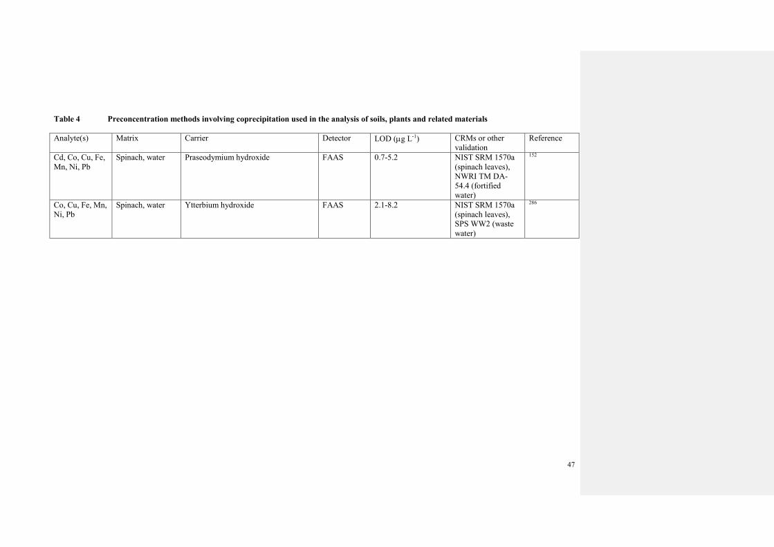
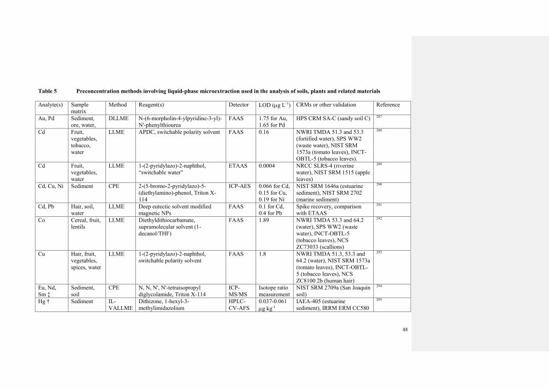
3.2.2 Sample preconcentration



4

3.3.2 Atomic emission spectrometry

3.3.3 Atomic fluorescence spectrometry


3.3.5 Accelerator mass spectrometry

3.3.6 Thermal ionisation mass spectrometry



4 Analysis of geological materials

4.1 Reference materials and data quality

4.2 Solid sample introduction

4.2.1 Laser ablation inductively coupled plasma mass spectrometry


4.3 Sample dissolution, separation and preconcentration


4.4.1 Atomic absorption and emission spectrometry


4.4.3 Other mass spectrometric techniques

4.4.3.1 Thermal ionisation mass spectrometry

4.4.3.2 Secondary ion mass spectrometry

4.4.3.3 Accelerator mass spectrometry

4.4.3.4 Noble gas mass spectrometry


5 Glossary of terms

6 References

5

1 Air analysis

1.1 Review papers

Review papers summarised current and emerging technologies for the detection,

characterisation and quantification of inorganic engineered–nanomaterials in complex

samples7 (217 references) and, upon their release, into the wider environment8 (80

references). An interesting review of laser-based techniques 9 (180 references) covered the in-

situ characterisation of tailored nanomaterials, synthesised from gas-phase precursors.

Progress in the analysis of nanomaterials for toxicological purposes was reported10 (91

references), as was the suitability of methods to measure solubility11 (116 references), an

important physiochemical parameter within emerging nanoregulation. In a thought–

provoking review12 (53 references), the question “do ICP-MS based methods fulfill the EU

monitoring requirements for the determination of elements in our environment?” was

answered in the affirmative but it was considered that challenges such as sample

contamination, robust implementation of suitable QA/QC programmes and lack of

harmonisation in the reporting of data remained. Other useful review papers summarised new

environmental applications of ICP-MS/MS13 (54 references), progress in PIXE for the

analysis of aerosol samples14 (24 references), analytical approaches for the determination of

As in air15 (139 references), emerging applications for a new SEM-EDX/Raman

spectroscopic system within environmental, life and material sciences16 (45 references) and a

review on field-based measurements 17 (110 references) which discussed the advantages and

limitations in the use of portable instruments for environmental analysis.

1.2 Sampling techniques

Particle–collection efficiency is an important consideration in selecting suitable filter

media for workplace air monitoring. New data for commonly used filters confirmed18 that

MCE, PTFE and PVC filters have relatively high collection efficiencies for particles much

smaller than their nominal pore size and are considerably more efficient than polycarbonate

and Ag–membrane filters. Personal air samplers designed to collect NPs (nanodeposition

samplers) often use nylon meshes to trap small particles but porous polyurethane foam was

considered19 a suitable alternative with low elemental impurities and good collection

efficiencies. Although large particles (30-100 µm) found in workplace air can be inhaled,

commonly used size-resolved samplers, such as cascade impactors, are generally limited to

handling particles sizes of <20 µm. Two new prototype samplers capable of collecting larger

6

particles were based20 upon the principles of a vertical elutriator and it will be interesting to

watch their future development.

Evaluation of the performance of impactor samplers continued to be reported. Two

ISO methods for the in-stack sampling of both PM2.5 and PM10 employing both conventional

and virtual impactors were compared21 by use both in the laboratory and in the field at a coal-

fired plant. The conventional impactor performed worse as it overestimated PM2.5

concentrations due to particle bounce and re-entrainment even when an adhesive coating was

applied to the impaction plates. Collecting sufficient sample mass for detailed chemical

characterisation in supporting health effects studies requires air samplers operating at

substantially higher flow rates than the 1–2 m3 h–1 typically used currently. The design and

validation of two new high volume PM2.5 impactors operating at 57 and 66 m3 h-1 has been

reported22, 23 as has a new impactor design24 that can sample either PM1 or PM2.5 at a nominal

10.5 m3 h-1 flow rate.

Continuous analytical systems are proving useful for the time-resolved measurements

of aerosol chemical composition which are needed to elucidate a greater understanding of

atmospheric processes and reactions. With the objective of unattended continuous long-term

weekly sampling of size segregated ambient particulate matter, a sampling system25

consisting of a modified 3-stage rotating drum impactor in series with a sequential filter

sampler was used to collect <0.36 µm, 0.36–1.0 µm, 1 .0–2.4 µm and 2.4–10.0 µm particle

size fractions. Accumulated sample deposits were subsequently analysed either by thermal

desorption GC-TOF-MS (organic species) or by XRFS (elemental species). The sequential

spot sampler is a design that uses a water-based condensation growth technique to grow fine

particles into µm-sized droplets which can subsequently be impacted as dry spots. In one

particular design26, impaction of a droplet resulted in a sample spot of ~1mm diameter within

a well of a 96 place collection plate. Subseqent droplets were deposited sequentially in clean

wells thereby facilitating the collection of time-resolved air samples. In one application of

this new system, a multi-well plate recovered from the field was processed in the laboratory

wherein each spot was extracted with water and analysed by IC for its nitrate and sulfate

content. This multi-well plate approach has good potential as the plates could potentially be

incorporated in a range of instrumental autosampler systems thereby facilitating automation

of extraction and analysis. The semi-automatic measurement27 of soluble Cu and Pb in

atmospheric samples was achieved by coupling a deposition sampler to an ASV detection

system that employed screen-printed electrodes. In a one-month field study, this approach

proved reliable with low ng L-1 LODs. Successful validation involved analysis of water

Formatted: Highlight

7

CRMs and comparison with data obtained by ICP-MS analysis. The fate of anthrogeneic Hg

emissions in the atmosphere is influenced by the exchange of Hg0 with the earth surface but

the accurate determination of Hg0 fluxes has proved technically challenging as airborne

concentration differences between up-draughts and down-draughts can be very small (<0.5 ng

m-3). An improved REA system28 built around a single AFS detector system had twin-inlets

and pairs of Au preconcentration cartridges for the concurrent sampling and analysis of Hg0

in both up and down-draughts. This sophisticated system possessed a Hg0 reference gas

calibration generator that enabled instrumental drift to be monitored and, if necessary, re-

calibrations to be undertaken.

Interesting new biosampler systems have been proposed. After a gun is fired, gun shot

residue deposited on a shooter’s hand disappears gradually through washing or contact with

surfaces so detection on skin is limited by the need to sample within eight hours of the firing.

Particles trapped within nasal mucus however had29 potentially longer residence times.

Swabbing with an EDTA-wetted cotton bud and digestion in acid was all that was needed to

prepare samples. Particle concentrations were lower than those found in hand swab samples

but this was not an issue if a sensitive technique such as ETAAS were employed. Progress

continued30 in the LA-ICP-MS measurement of the isotopic composition and concentration of

Pb in the dentine and enamel of deciduous teeth which gave a record of historical UK Pb

exposure during fetal development and early childhood. Children born in 2000, after the

withdrawal of leaded petrol in 1999, had lower dentine Pb concentrations than children born

in 1997 and an isotopic ratio fingerprint that correlated very closely with modern day

Western European industrial PM2.5/10 aerosols. In contrast, for those born in 1997, the isotopic

ratio fingerprint was a binary mixture of industrial aerosols and leaded petrol emissions.

Exhaled breath condensate (EBC), the condensate from exhaled breath during regular tidal

breathing, has been proposed31 as a useful medium which, when used alongside established

urine biomonitoring, can give a more comprehensive picture of worker exposure to CrVI.

Collection used a portable sampler similar to a breathalyser with a peltier cooler unit for

condensation of the exhaled breath. Single–use mouthpiece, plumbing and clean test tubes

were used for each sample taken. The EBC was diluted ten-fold with an EDTA solution and

analysed by microbore LC-ICP-MS. The Cr speciation profile in spiked EBC samples could

be maintained for up to 6 weeks if stored at 4 °C but not if samples were frozen.

8

1.3 Reference materials and calibrants

Reference materials (thin film standards) available for calibration of XRFS do not

necessarily mimic real-world filters collected in air quality monitoring programmes. New Pb

reference filters were generated32 by mounting air samplers, with the appropriate filter

substrate, within an enclosed aerosol chamber and challenging them with Pb-containing

aerosols produced from ICP-grade standards using a desolvating nebuliser. Filters were

prepared to mimic mass loadings typically found in surveys and equivalent to airborne

concentrations of between 0.0125 and 0.70 µg m-3. Extension of this work in preparing filters

with other elements is now underway. Methods for the generation of test Pb or PbO NPs

involved33 either the thermal decomposition and oxidation of lead bis(2,2,6,6,-tetramethyl-

3,5-heptanedionate) or the evaporation and condensation of metallic Pb. The latter approach

was deemed to be more suitable due to its simplicity, high production rate and the well-

defined composition of the NP formed. A novel porous tube reactor33 facilitated the

production of NPs from the gas phase and offered a controlled process for the synthesis of

ultrafine metal particles with subsequent oxidation and dilution steps. Magnetic Fe and

maghemite were synthesised using Fe pentacarbonyl as a gas-phase precursor and NPs with

primary particle sizes of 24 and 29 nm and geometric mean diameters of 110 nm and 150 nm

produced. Data agreed well with those derived from modelling which, for Fe NPs, predicted a

primary particle size of 36 nm and an agglomerate size of 134 nm.

The generation and testing of gas standards is of widespread interest. High purity

nitrogen or air, often referred to as “zero gas”, is essential as a blank standard for calibrating

instruments used in air quality monitoring. Providing traceable and accurate quantification of

impurities in such gases is challenging as the LODs of analytical techniques required are

often similar to the concentrations of the measurands in question. A useful review paper34 (21

references) described the status of the measurement science and available data on the

performance of a selection of zero air generators and purifiers. Although gas standards in

pressurised metal cylinders are popular, there is potential for selective adsorption onto the

metal surfaces. In a new study35 on the reversible adsorption process between trace species –

CH4, CO, CO2 and H2O – and cylinder surfaces such as aluminium and steel, the authors

recommended that for highly precise trace gas analysis aluminium cylinders should be used,

temperature fluctuations should be minimised to limit desorption and diffusion effects and

cylinder usage should be restricted to units pressurised above 30 bar.

9


In a microwave-assisted extraction procedure36 for the speciation of SbIII and SbV in

PM10 airborne particles collected on quartz fibre filters, leaching with 0.05M

hydroxylammonium chlorohydrate solution was recommended. This new approach

recovered spikes quantitatively and extracted more Sb from samples than the hither–to used

ultrasonic extraction procedure. Optimal digestion conditions37 for the dissolution of TiO2

NPs collected on air filter samples involved the use a H2SO4:HNO3 acid mixture (2:1 v/v)

heated to 210 °C.

An operationally defined sequential leach procedure38 for Mn speciation in welding

fume involved four-steps: a 0.1M ammonium acetate leachate for soluble Mn components; a

25% (v/v) acetic acid leachate to dissolve Mn0/II species; a 0.5% (w/v) hydroxylamaine

hydrochloride in 25% (v/v) acetic acid leachate to dissolve MnIII/IV species and a final HCl-

HNO3 acid mix to digest the residue. Recoveries for test samples consisting of pure Mn

compounds (Mn nitrate solution, Mn powder, MnII/IIIoxide) were in the range from 88 to

103%. A SiMn alloy and two certified welding fume RMs were subsequently tested but in

these cases total Mn recoveries were only 68–75% suggesting, in this reviewer’s opinion, that

the final acid digestion step was not agressive enough. Analysis of fumes derived from flux

welding demonstrated that the dominant forms were Mn0/II and insoluble Mn. For fume

derived from an arc weld process, the dominant form was the MnII/IV fraction. Interested

readers are referred to a review39 (112 references) on Mn speciation.

New approaches for the preparation of particulate samples for subsequent

instrumental analysis included tangential flow filtration used40 to preconcentrate black carbon

particles from ice-water, remove matrix salts and limit particle aggregation, prior to TEM

analysis. The continuous flow of sample solution tangentially across a filter membrane not

only minimised particle clogging but also facilitated the filtration of unwanted dissolved

matrix salts. The interrogation of aerosol samples is often challenging due to the limited

sample quantity available. The use of an automated graphitisation equipment enabled41 small

quanitities of carbon-containing particulates, collected on quartz filters, to be converted

effectively into a graphite target for subsequent AMS analysis. Recoveries were >80% and

reproducible C14 values were obtained for sample masses in the range 50-300 µg. Strategies

for the preparation of samples for LIBS have been reviewed42 (145 references). A new

micromanipulator system43 facilitated a better handling of radioactive fall-out particles found

in sediment samples prior to analysis using SEM and SR techniques.

10


1.5.1 Atomic absorption, emission and fluorescence spectrometry

The direct analysis of particles remains attractive as onerous sample preparatory steps

can be minimised or even eliminated. The determination44 of Cl in pulverised coal samples

using solid sampling HR-CS-AAS exploited the characteristic molecular absorption of the

SrCl molecule at 635.862 nm. Under optimised conditions of pyrolysis at 700 °C and

atomisation at 2100 °C, the LOD and Mo were 0.85 and 0.24 ng, respectively. Results for

five, well homogenised, coal CRMs (BCR 180,181,182 and NIST SRM 1630a and 1632b)

agreed with certified values. Refreshingly, the authors concluded however that similar

analytical performance may not be possible for coarser-grained real-world coal samples given

that the proposed method consumed a sample mass of only ~0.15 mg. They suggested that

one possible option would be to increase the sample mass taken for analysis in conjunction

with the selection of a less sensitive molecular transition line. In a fast screening method

involving ETV-ICP-AES45, P, S and Si impurities in Ag NPs were determined at a rate of 35

samples per hour. The important point in this proposed method was that the entire sample

could be vaporised thereby enabling simultaneous measurement of the emission from both

the impurity elements and the Ag matrix. No tedious weighing procedure was therefore

required. The LODs for P, S and Si in a dry powder Ag matrix, were 4.2, 62 and15 µg g-1,

respectively.

A commercially available AFS analyser was modified46 to undertake airborne

measurements of atmospheric Hg as part of the ongoing CARIBIC project. Salient features

included the use of: two Au cartridges to achieve continuous sampling (while one was

sampling the other was being desorbed); a pressure-stabilised AFS detector cell to ensure a

stable detector response; and a molecular sieve to remove the 0.25 % (v/v) CO2 from the

argon carrier gas as this would otherwise have quenched the AFS signal. In an attempt to

minimise the number of calibrant gases taken on board, this gas supply was also used to

calibrate the onboard CO2 gas analyser.

Developing LIBS as a quantitative technique is a goal that is shared by a number of

research groups. Ideally the measurement requirements are that the sample be completely

dissociated and diffused within the plasma on time-scales conducive with analysis thereby

resulting in analyte emission at the bulk plasma temperature with a signal that is linear with

mass concentration. Following experiments involving the interrogation of multi-elemental

test aerosols, it was concluded47 that local perturbations of plasma properties can occur so

significant analyte-in-plasma residence times (tens of µs) were therefore necessary. Another


11

study48 concluded that the goal of achieving accurate compositional measurements without

the use of calibrants was only possible if the delay between the laser pulse and the detector

gate ramained short, i.e. <1 µs. Investigations into the use of on-line LIBS for the elemental

analysis of powered coals have been reported49,50. In the first paper49, a tapered sampling tube

was useful both for enriching the coal particles within the laser focus spot (another design

goal when applying LIBS to the analysis of aerosol samples) and to reducing the influence of

air entrainment and fluctuations in plasma conditions. In the second paper50, on the influence

of omnipresent moisture, it was concluded that part of the laser energy could indeed be

expended on ionising the surrounding water vapour. This resulted in less coal mass being

ablated and consequently in lower emission intensities. For more information on fundamental

developments in atomic spectrometry readers are directed to our companion ASU3.

1.5.2 Mass spectrometry

1.5.2.1 Inductively coupled plasma mass spectrometry. The advent of a new ICP-MS/MS

instrument has encouraged development of new applications. In one51, three cell modes:

single quadrupole (Be, Pb and U); MS/MS with NH3-He (Co, Cr) and MS/MS with O2 (As,

Cd, Mn, Ni and Se) were used for quantification in cigar smoke. The elimination of unwanted

interfering isobaric ions was achieved using a shifted analyte masses mode (via ammonical

clusters or oxides) which gave better LODs than those obtained with a single-quadrupole

ICP-MS instrument. For example, the LOD for Mn was reduced from 13 µg g–1 to <3 µg g–1

and that for Se from 0.7 µg g–1 to <0.02 µg g–1. In a somewhat unusual study52, ICP-MS/MS

was used to study the abiotic methylation reaction of inorganic Hg with VOCs. Several

VOCs (acetic acid, ethyl acetate, methyl benzene and methyl iodide) reacted with Hg to form

methyl Hg at a conversation rate of 1-2%. One is left to ponder whether ion chemistry within

an ICP-MS system can be truly representative of atmospheric processes but also whether this

rather innovative approach involving an alternative use of an ICP-MS system could be useful

for studying other gaseous reactions. A useful tutorial review13 (55 references) describing this

new instrument has been published.

Speciation applications involving the use of HPLC-ICP-MS included53 the coupling of

AEC to ICP-MS for the simultaneous speciation of chromate, molybdate, tungstate and

vanadate in alkaline extracts of welding fume. At the high alkalinity conditions employed, the

CrO42-, MoO4

2- and WO42- species gave single sharp chromatographic peaks but the peak for

VO43- was slightly broader. The LODs ranged from 0.02 ng ml-1 for CrO4

2- to ca. 0.1 ng ml-1

for the other measurands. Method accuracy was checked using either IRMM CRM 545 (CrVI

12

in welding fume loaded on a filter) or, for the other analytes, spiked samples. Results for Cr

were within the certification range and spike recoveries were 98-101%. Five As species

(AsIII, AsV, MA, DMA and TMAO) in water extracts from air filter samples were

determined54 by HPLC-HG-ICP-MS. The total extractable As content was 0.03–0.7 ng m-3

and the relative abundance in the sequence AsV > TMAO > DMA > AsIII > MA. There were

no discernable seasonality effects although TMAO concentrations were higher in winter

samples than in summer samples. In a similar study55 on the extraction of As species, up to

54% of an AsIII spike added to extracts was oxidised to AsV. This finding emphasised the

challenge of converting laboratory-based speciation science into real-world applications

where such transformations can occur readily.

The LA-ICP-MS technique enables swift interrogation of particles with minimal

sample preparation but further work is required to develop calibration strategies for

quantitation. One proposed approach56, involving the use of MC-ICP-MS, offered a rapid,

accurate and precise method for the determination of isotopic ratios in U-containing particles.

The methodology involved the use of adhesive–tape–sampling to fix particles, SSB to correct

for mass fractionation effects and repeat analysis of suitable CRMs such as NBL CRM 124-1

(U3O8 24 element impurity standard) and NRCCRM GBW 04234/04236 (U isotopic

abundance in UF6). The relative uncertainties in 235U/238U, 234U/235U and 236U/238U

measurements were <0.05, 1.7 and 1.8%, respectively, and the isotopic ratios determined

were in good agreement with certified values. A new procedure57 for the determination of the

trace element content in powdered environmental samples did not require matrix-matched

CRMs. Powdered samples were mixed with an AgO internal standard and a Na2B4O7 binder

and pelletised. Powdered CRMs with varying matrix composition and analyte content were

prepared and analysed in the same way for quantification. Applicability of the procedure was

demonstrated by the successful quantification of As, Cu, Ni and Zn in four different matrix

CRMs: NIST SRM 1648a (urban particulate matter); NIST SRM 2709 (San Joaquin Soil);

IRMM CRM 144 (sewage sludge) and IRMM CRM 723 (road dust). Three of these materials

were used as calibrants and the fourth analysed as an unknown sample.

Using an ICP-MS instrument as detector for the on-line measurement of particles is a

fertile, interesting but challenging research area. Researchers in Austria described58,59 a

system for measurement of the time-resolved release of Cl, K, Na, Pb, S and Zn from single

particles during biomass combustion. Researchers in Switzerland developed60 a SMPS-ICP-

MS system coupled with a rotating-drum device for the simultaneous determination of both

the size distribution and elemental composition of NPs. Meanwhile in the Czech Republic,

13

researchers used61 substrate-assisted laser desorption to introduce Au NPs from a plastic

surface into an ICP-MS instrument. A 61% transport efficiency was achieved using 56 nm-

sized reference NPs. In a more fundamental study62, particles (Al2O3, Ag, Au, CeO2 and

Y2O3) in the 100-1000 nm size range were injected into an ICP-MS system in order to

calculate relative detector response factors. The response factors ranged between 10-5 and 10-

11.

1.5.2.2 Other mass spectrometry techniques. Developments in other MS techniques for

gaseous analysis included a new analyser63 for the speciation of trace levels of atmospheric

oxidised Hg compounds, required to gain a better understanding of the biogeochemical cycle

of Hg. The system consisted of an ambient air collection device (either nylon membrane or

quartz wool substrate), a TD module, a cyrofocusing system and a GC-MS analytical system.

A permeation-based calibration system with an associated AFS detector provided stable and

quantifiable amounts of gas-phase Hg0, HgBr2, HgCl2, Hg(NO3)2 and HgO calibrants. In a

laboratory setting, this instrument could be used to speciate HgX2 compounds at an

instrumental LOD of 90 pg but it was not possible to ascribe unequivocally mass spectra to

either Hg(NO3)2 or HgO species. In field use, the LOD was 10–18 pg m-3 but no oxidised Hg

species could be detected when air samples were analysed. It was concluded that either a

lower LOD was required or that species transformation during sampling occured. Future

work in this most challenging field will include the testing of more inert sample collection

substrates and the use of alternative MS detectors. A GC-MS method64 achieved LODs of 3.3

x 10-8 (V/V) and 2.6 x 10-9 (V/V) for atmospheric Kr and Xe gases, respectively, with a

relative standard uncertainity of ca. 3%.

Improvements in isotope ratio-MS included a fully automated system65 for the

determination of ∆13C and ∆18O in atmospheric CO samples which used Schutze reagent

(I2O5 on silica gel) to convert extracted CO to CO2. Use of high–purity He to flush

continuously the instrument system resulted in low but constant system blank signals that

were <1-3% of typical sample signals. The measurement repeatability was <0.2% and a

single measurement took 18 minutes. A commercial GC-isotope ratio-MS system modified66

for on-line carbon ID used a constant flow of CO2, enriched in 13C and diluted in He, added

via the flow splitter located within the chromatography oven. The precision for isotopic ratio

measurements was ca. 0.05% RSD (n = 50). The relative abundances of N2O isotopocules

(molecules that have the same chemical constitution and configuration and only differ in

isotopic composition) are potentially useful tracers for understanding the atmospheric

14

production pathways, sinks and decomposition reactions of N2O, an ozone-depleting gas. A

new automated sample preparation system67 able to accommodate flask samples that previous

systems could not handle consisted of a sample injection unit, a cyrogenic concentration unit,

a purification unit and a cryofocusing unit, all mounted on a compact mobile trolley that

could be wheeled into place and connected to the IRMS instrument. A sample could be

processed in 40 minutes. The precision values of <0.1‰ for ∆15N and <0.2‰ for ∆18O were

comparable to those obtained with other automated but less mobile systems and better than

those obtained using manual off-line preparatory systems.

Developments in MS techniques for analysis of airborne particulates included a

newly developed LA-TOF-AMS system68 that consisted of two 405 nm scattering lasers for

particle sizing, a 193 nm excimer laser for ablation/ionisation of particles and a TOF-MS

detection system with a mass resolution of m/∆m >600. Laboratory tests gave a maximum

detection efficiency of 2.5% for particles with a nominal diameter of 450 nm.

A particle trap laser desorption mass spectrometer69 for the quantification of SO42-

aerosols gave results highly correlated (r2=0.96) with but consistently lower than those

obtained using a more conventional thermal decomposition/oxidiser system coupled to a SO2

gas sensor. These discrepancies were explained by differences in the respective sampling

inlets and differences in the vaporisation efficiencies of particles since the laser desorption

MS system was operated at ~500 °C whereas the thermal decomposition analyser ran at 1000

°C.

The Aerodyne aerosol mass spectrometer is a commercially available and frequently

used instrument for the on-line measurement of sub-µm ambient aerosols. Two papers

described work undertaken to understand better the performance of this instrument. In the

first70, an instrument was challenged with test aerosols ranging from NH4NO3 (non-

refractory) to ZnI2 (semi-refractory) in order to gain a better understanding of how well

particles vaporised at ~600°C. It was concluded that the W vaporiser unit did not always

behave inertly towards particles, that no sharp separation between non-refractory and

refractory species was possible and that, as a result, measurements of semi-refractory aerosols

could indeed be biased. The second paper71 addressed errors inherent in the fitting and

integration of ion peaks that could be an appreciable source of potential measurement

imprecision. Coupling of the Aerodyne aerosol mass spectrometer with a Nd:YAG laser

(from a single particle soot photometer) to produce an instrument known as the soot-particle

aerosol mass spectrometer which could be used to measure atmospheric particles including

refractory black carbon (rBC) species. A method72 for the detection and quantification of the

15

trace metal contents of soot particles involved preparing synthetic calibration standards by

dosing suspensions of carbon black particles with various concentrations of aqueous metal

spikes. The resultant standards were then nebulised, dried and directed through a differential

mobility analyser to generate a monodispersive (300 nm) test aerosol (i.e. dried carbon

particles coated with trace metals) for soot particle-aerosol MS. In an initial field trial

conducted in the vicinity of an oil fired power station, qualitative mass spectra data revealed

evidence for metallic oxide and sulfate species. The Ba, Fe and V data agreed, within a factor

of 2, to those obtained using the ICP-MS of filter samples taken at the same time.


The analysis of particles on filters by XRFS is now well established but new

approaches are always welcome. One feasibility study73 investigated whether it would be

possible to analyse particles collected using the StreakerTM sampler by EDXRFS rather than

by the more conventional PIXE approach. In this ambient air sampler, a filter is rotated at a

constant rate under an incoming stream of particle-laden air thus forming a continuous streak

which provides time-resolved elemental air concentration data. A customised XRF

instrument with a focused but small collimated beam provided data as good as those obtained

by PIXE analysis. Irregular dust depositions on 25-mm diameter filters mounted in the widely

used IOM inhalable workplace dust sampler can pose difficulties when attempting elemental

quantification using pXRFS instruments which, by their design, have intrinsically small X-

ray beams. Averaging four filter readings, obtained by manual rotation of filters by quarter

turns, yielded74 Pb results that were within –28% and +38% of results obtained previously

using a laboratory-based WDXRF system. The latter possessed a wider X-ray beam that

could illuminate the whole filter and an automatic sample spinner to average out

heterogeneities in dust deposits on filters. Measurement of Pu fall-out particles in soil

matrices is of interest to those working in nuclear safeguarding, forensics and remediation

activities. In a powerful demonstration75 of advances in analytical capabilities, the elemental

composition of two Pu–contaminated soil samples was characterised using both high

resolution µXRFS and 3D confocal XRFS. The LOD was <15 pg for samples with a nominal

30 µm grain size. Complimentary morphologic and sizing information was available using X-

ray transmission microscopy and micro X-ray tomography.

The solid state speciation of airborne particles provides powerful new information on

the composition of individual particles. The analysis of PM10 and PM2.5 by XANES and XRD

confirmed55 the presence of Ca3Sr2(AsO4)2.5(PO4)0.5(OH), As2O3 and As2O5 species. An

16

understanding of Cs speciation in dust emissions from either municipal solid waste

incineration (MSWI) or sewage sludge incineration (SSI) is important when considering

disposal options of waste which may be contaminated with low levels of radionuclides.

Analysis by µXAS confirmed76 that Cs speciation in MSWI dust was best described as a

potentially soluble CsCl2 species but that in SSI dust it was best described as an insoluble

pollucite material, a zeolitic structure with a typical composition of Cs2Al2Si4O12.2H2O.

Mercury can be associated with fly ash in emissions from coal-fired power stations. The

µXAS analysis of a simulated flue gas showed77 that Hg was associated with Br and Cl, could

be bound to Fe oxides and could also occur as a cinnabar (HgS) species. This information

would be most useful for those tasked with the safe disposal of Hg–containing fly ash.

Nuclear forensics makes use of tools such as XAS but reference spectroscopic signatures for

a range of U compounds in the soft X-ray spectral region are required. A new study78

compiled suitable reference spectra into a useful searchable database for a variety of common

uranyl-bearing minerals including carbonates, oxyhydroxides, phosphates and silicates.

Interested readers are invited to read our companion XRF ASU5 to learn more about

instrumental developments and potential applications.

1.5.4 Other analytical techniques

Commercially available field-based IC-based systems that measure, in near real-time,

water soluble airborne ionic species are useful in gaining a better insight that such species

play within atmospheric processes. In these systems, particles are sampled, hydrated in a

steam generator and the resultant water–soluble ions extracted and analysed using IC. It is

also possible to separate gas-phase ionic species from particles that contain ionic species by

using denuder technology. There is now a need to compare data generated using these new

systems with data generated using more established laboratory-based IC methods to ensure

continuity in monitoring data sets. One study79, conducted at an urban location, compared

hourly in situ data with data derived from 24 h filter samples returned and analysed back in

the laboratory. Overall, data correlated well for Cl-, Mg2+, NH4+, NO3

- and SO42- (r2 >0.83)

but less so for Ca2+, Na+, K+ (r2 <0.5). On average, the in-field approach gave substantially

higher concentrations for K+, Na+ and NH4+ than those measured in the laboratory. In a

second study80, conducted at a rural location, online measurement of NH4+ concentrations

compared favourably with off-line measurements (r2 >0.83, mean differences <6%). The

SO42- concentrations determined online correlated well with off-line measurements (r2 >0.84)

but with mean differences of up to 35%. In the case of NO3-, the correlation was poor (r2

17

<0.1) and the mean difference could be as great as 520%. Performance differences could be

attributed to a number of factors including: differences in the particle size selectivity of the

respective sampler inlets; collection efficiencies and volatility losses within the steam-jet

aerosol collector; instrument saturation effects; sampling artifacts (both positive and

negative) in the off-line filter sampling method; and challenges and uncertainities in

measuring low airborne concentrations of species such as K+. Nevertheless, such studies are

most informative as the air monitoring community slowly transitions from laboratory-based

to field-based measurements. Modification of a particle-into-liquid sampler coupled with IC

led81 to a dramatic increase in performance. Twin ion exchange pre-concentration cartridges

(one for cationic and one for anionic species) were inserted so that one sample could be

enriched while the preceding one underwent chromatographic separation and analysis. This

gave a 10- to 15-fold improvement in LOD and, importantly, a 24-fold increase in live time

coverage from 2 to 48 minutes in every hour.

A TD carbon analyser82 used with a cavity ring-down spectroscopy system enabled

isotope ratio measurements to be performed on carbonaceous particulate matter. The data

were in reasonable agreement with values previously reported in the literature. The precision

was <1.0‰. This study demonstrated the potential of the new system as an alternative to the

established IRMS measurement approach. Assessing the containment performance of storage

wells in carbon capture schemes requires time-resolved measurements taken at locations

around potentially large sites together with the use of isotopic CO2 tracers. Use of IRMS is

not feasible but the use of a CRDS system equipped with a gas sampling manifold system has

been advocated83. A H2S interference84 which biased 12CO2 measurements high and 13CO2

measurements low was overcome by installing a scrubber packed with Cu filings to remove

H2S selectively as samples entered the instrument. A CRDS system, modified for use in

flight, was used85 to make NO2 measurements over the eastern seaboard of the USA.

Instrumental calibrations were linear up to 150 nM. The LOD was 80 pM. The remarkably

consistent airborne concentrations (~3×1015 molecules cm–2) from ground level up to an

altitude of 2.5 km indicated that NO2 was widely but uniformly distributed in the air over the

eastern USA.

There is growing interest in the use of quantum cascade lasers for gas monitoring

applications as these systems can be portable, sensitive and selective and provide rapid

analysis. A preconcentation unit, in which electrical cooling rather than the more

conventional liquid N2 cooling was used, trapped86 CH4 but not other major components (e.g.

N2 and O2 ) or interferents (e.g. CO2 and N2O). The preconcentration factors of up to 500


18

resulted in an analytical precision of 0.1‰ for ∆13C and 0.5‰ for ∆D-CH4 based upon a

nominal 10–minute instrumental integration. The average differences in results obtained by

this new approach and the currently used approach of Dewar sampling and IRMS were within

the WMO compatability goals of 0.2‰ for ∆13C and 5.0‰ for ∆D-CH4. Use of a new

pressure-corrected calibration protocol reduced uncertainties in the airborne measurement87

of CH4 and N2O to ±2.47 and ±0.54 ppb (2 σ), respectively.

The use of thermal-optical analysis for measuring the carbonaceous content in

atmospheric particles is well established. Addition88 of a multi-wavelength capability to an

existing instrument, made possible by recent advances in laser diode technology, should

provide better optical interrogation of filter samples in the furnace as they undergo

combustion and thereby provide improved identification of the source of carbon. A method89

for calculating equivalent black carbon concentrations from elemental carbon data derived

from thermo-optical analysis will make it easier to compare data derived from combustion-

based and optical-based measurement systems. Determination of the organic carbon content

of atmospheric particles, measured using a thermal-optical approach90, made use of an

empirically-derived organic carbon volatility model. Data for this model were obtained from

paired samples: quartz fibre filters that collected all organic carbon species; and quartz fibre

filters mounted behind Teflon filters that collected volatile organic species but not

particulate-bound organic carbon species.

Other instrumental developments and applications included an INAA method91 for

measurement of 37 elements in particles trapped in ice core samples. Reduction in

background instrumental noise resulted in a 1-3 order of magnitude improvement in LOD,

equivalent to absolute LODs in the range 10-13 to 10-6 g. Raman spectroscopy92 was the basis

of a new continuous soot monitoring system used to provide the first diesel fume

measurements in a controlled environmental chamber. Future work will include the use of

multivariate data analytics to interrogate spectral information as well as the optimisation of

instrumental hardware to improve sensitivity. The potential of the EBS and PESA techniques

for measuring low Z-elements such as C, H, N and O collected on PTFE filters was

evaluated93. Direct measurement of organic or elemental C was not possible but it was

suggested that H could be used as a proxy for organic C and that the elemental C fraction

could then be calculated as the difference between total C and this organic C fraction. A non-

destructive, fast and inexpensive FTIR approach94, 95 could be used to predict the levels of

organic and elemental C in particulate matter collected on PTFE filters. The FT-IR spectra

were calibrated, via PLSR, using OC/EC data obtained from the thermal combustion analysis

19

of particulate matter sampled in a similar way but on quartz filters. Automated particle

screening software96, developed for SIMS analysis, enabled those few U particles with

irregular isotopic composition to be identified and to be isolated for further TIMS analysis.

1.5.5 Intercomparisons and data analytics

Laboratory intercomparison exercises can be most useful in assessing the

performance of new methodologies and instrumentation. A study97 evaluated how well

laboratories performed in dissolving new acid-soluble cellulose-based air sampling capsules

designed to sample metals in workplace air. Capsules were spiked, at three loadings, with 33

elements in the range 2–100 µg per sample and triplicates sent to each of eight laboratories. A

variety of hotblock, hotplate and microwave–assisted digestion protocols were used to

prepare the test samples for analysis by ICP-AES. For 30 of the 33 elements the NIOSH

accuracy criterion of results not deviating by >25% from spiked value was achieved. The

elements that presented difficulties were Ag (potential for precipitation in chloride–based

solutions), In (low instrumental sensitivity) and Sn (passivation in oxiding acids). Data from

this study supported the development of the new NIOSH 7306 method. Laboratories

employed98 EDXRF (using both external calibration and FP approaches) and PIXE

methodologies in a comparative study of the measurement of elemental loadings on PM10

filter samples. The NIST SRM 2783 (air particulate on filter media) was analysed by all

laboratories to provide data for comparison. Further data were obtained by digesting

representative filters in HF using a microwave procedure for ICP-MS analysis. The data for a

range of elements (Br, Cu, Fe, K, Mn, Pb, S, Sr and Ti) were consistently within 20% of each

other. Data were also comparable with those obtained by ICP-MS except for those for Fe and

Zn. Cross-contamination was a possible explanation for these discrepancies. In summary, the

authors concluded that it was possible for laboratories with different instruments, setups and

calibration approaches to make comparable measurements on filter samples.

Undertaking instrumental intercomparisons in the field can be both time consuming

and logistically challenging! In a comprehensive exercise99, 47 CRDS instruments were

tested to assess their performances for measuring atmospheric CH4, CO, CO2 and H2O

species. Only 15 instruments were actually tested in the field following an initial screening in

the laboratory. As might be expected, newer models performed better than older ones and the

overall recommendations included: instrument performance should be verified in the

laboratory using a standardised protocol before deployment in the field; instruments should

be stabilised for 10 minutes prior to undertaking measurement; in the field calibrations should

20

be performed initially every 2 weeks for the first 6 months and subsequently after every

instrument restart. The first ever large scale intercomparison100 of aerosol mass

spectrometers, carried out at a field station outside Paris, took 3 weeks to complete. The first

week was dedicated to instrumental set-up, tuning and calibration and then comparative

studies took place in the second and third weeks. Chemical species (ammonium, chloride,

nitrate, organic matter and sulfate) in the non-refractory sub PM1 fraction were measured

using 13 different instruments. Taking the median as a reference value, correlations were

strong (R2>0.9) for all systems across all measurands except chloride for which correlation

was poorer. It was suggested that this was due to instrumental sensitivity issues when

attempting to measure low atmospheric concentrations. Recommendations included guidance

on how best to perform calibrations and standardised protocols for data processing.

In two interesting studies, elemental ratio data have been used to track potential

emissions from specific industrial point sources. In the first101, La/Ce ratios were determined

in PM2.5 filter samples taken from the vicinity of petroleum refineries as these elements are

characteristic emission tracers from fluidised-bed catalytic cracker (FCC) columns. The use

of a high–throughput hot–block digestion for rapid ICP-MS analysis of 64 filter samples was

verified (80-90% elemental recoveries) using NIST SRM 1648a (urban particulate matter)

and SRM 2783 (air particulate on filter media). Subsequent modelling could not reliably

apportion measured PM2.5 to FCC emissions suggesting that the impact of refinery particulate

emissions on local air quality was minimal. In the second study102, Cd/Cu, Cd/Pb, Cr/Pb and

Cu/Pb ratios were determined in filters collected from the chimney stacks of six municipal

waste incinerators and at locations 10 km downwind. The stack samples, taken on quartz

fibre filters, were analysed by ICP-MS following a HNO3-HF microwave-assisted digestion

using the EN 14385 method. The ambient air PM10 samples, collected on cellulose filters,

were analysed by ICP-MS following a HNO3-H2O2 microwave-assisted digestion using the

EN 14902 protocol. Method performance checks used BCR CRM-038 (fly ash from

pulverised coal) and NIST SRM 1648A (urban particulate matter). There was no evidence of

emissions impacting upon local air quality around four installations and at the other two

installations the influence of emissions was minimal.

2 Water analysis

2.1 Sample preparation and storage

Two papers on oceanographic studies compared on–board sample preparation with

return of samples to the laboratory for processing. The first103 studied the partitioning of As,


21

Ba, Cd, Cu, Fe, Li, Mg, Mn, Pb, U, V and Zn between the dissolved and particulate fractions

in water samples from oceanic hydrothermal vents. When the samples were filtered on board,

results for dissolved fraction were higher than if the samples were sent back to the laboratory

for processing. As a consequence, results for samples taken back to the laboratory

overestimated the particulate fraction for all the elements studied. In the case of Fe, the

underestimation of the dissolved fraction was up to 96%. Although the measurement bias for

Li, Mg, Mn and U for the dissolved fraction of ≤3% was deemed acceptable, for all other

elements in situ filtration was necessary. The authors concluded that filtration after freezing

should not be used for deep sea elemental fractionation studies. In the second study104 on the

Hg isotopic composition of Arctic seawater, samples were collected and either pre-

concentrated on board immediately or stored in the dark and preconcentrated in the

laboratory. Samples preconcentrated in the laboratory had more positive δ202 Hg values than

those prepared on board, probably due to abiotic reduction of Hg in the dark by organic

matter during storage and shipment. A fractionation factor of 1.49±0.12‰ for δ202 Hg was

applied to correct for this effect.

The stability and degradation of elemental species under storage has been of interest

for a long time. In a study105 of the degradation of butyl tin compounds in surface waters,

where isotopically labelled DBT, MBT and TBT samples were stored in glass, polypropylene

or PTFE containers, both biodegradation and photolytic degradation were mechanisms for

species interconversion. Dealkylation was higher for samples stored in polypropylene bottles

than for those stored in glass or PTFE bottles. Storage in amber glass bottles in the dark at -

18°C resulted in little dealkylation after two weeks but after four months 19% of the DBT

spike was converted to MBT. No degradation of TBT was observed, however. Pillay and

Kindness106 re-confirmed that addition of EDTA to water samples helped to preserve As

species in the presence of up to 50 mg L-1 Fe and Mn but not in the presence of the same

amount of sulfide. Simulated pore water was spiked with 50 µg L-1 AsIII, AsV, DMAV and

MMAV and 100 µg L-1 monothioarsenateV and tetrathioarsenateV. Following addition of

EDTA to a final concentration of 0.025M, the samples were aliquoted into plastic vials and

stored at –20 °C. If only Fe and Mn were present, the species were preserved for up to 2

months but in the presence of S2- some of the As species degraded almost immediately.

2.2 Sample preconcentration and extraction

Reflecting the maturity of this field, review articles are written every year on various

aspects of sample preconcentration. This year was no different. Deng et al.107 (135

22

references) provided a comprehensive review on the application of preconcentration and

separation techniques in AFS, covering not only preconcentration but also separation

techniques such as CVG in various solid and liquid matrices. A review108 (76 references) on

the use of biosorbents for SPE of toxic elements in waters covered the use of algae, bacteria,

fungi and yeasts as new absorbents. Hagarova and Urik109 (60 references) reviewed new

approaches to CPE. They focussed on either speeding up or improving the selectivity of this

popular method for the determination of trace metals.

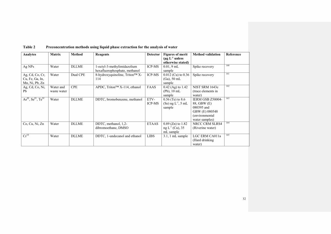
The most significant developments in analyte preconcentration for water analysis are

summarised in Tables 1 and 2.

2.3 Speciation and fractionation analysis

2.3.1 Review papers.

Most reviews of speciation analysis covered several matrices, including waters, but that110

(77 references) on Tl speciation was specific to water analysis. Recent advances in the

separation and quantification of metallic and ionic NPs were reviewed8 (80 references), as

was the use of NPs and nanoscale sorbents for the speciation of trace elements in the

environment111 (103 references). Mercury is always of interest and two reviews covered

sample preparation and quantification112 (90 references) and advances in separation and

detection techniques since 2013113 (157 references). Other reviews are included in the soils

and plants section of this ASU. For a broader overview of speciation analysis, the reader is

referred to our companion ASU114 (215 references).

2.3.2 Elemental speciation.

Faster separation was achieved115 for redox As species in river sediment pore waters by

operating an HPIC system at a flow rate of 400 µL min-1. Separation occurred within 4 mins

but analthough an additional 4 mins was required for effective column reconditioning. The

LODs with ICP-MS detection ranged from 0.05 (AsV) to 0.25 (MMAV). The accuracy of the

method was checked against the NRCC CRMs SLRS-4 (River water) and SLEW-3

(Estuarine water) and the sum of AsIII and AsV concentrations agreed with the certified total

As value. This method was considered to be suitable for the analysis of pore waters from

“poorly contaminated” sediment samples.

Methods for multielemental speciation are quite rare due to the compromise

conditions required. A Polish research group developed116 two chromatographic methods for

the separation of AsIII, AsV and CrVI in water, using a Hamilton PRP X-100 4.6 x 150 mm

23

normal bore anion-exchange column. Although both methods used isocratic elution at a

constant pH of 9.2 and a flow rate of 1.4 mL min-1, one method employed a mobile phase of

22mM (NH4)2HPO4 and 25mM NH4NO3 and the other 22mM (NH4)2HPO4 and 65mM

NH4NO3. The first mobile phase gave higher signal and a shorter analysis time (<3 mins for

elution of the analytes) whereas the second gave an improved separation resulting from the

longer elution time of 6 mins. The LODs with ICP-MS detection in reaction mode ranged

from 0.090 (AsV) to 0.16 (AsIII) µg L-1 for the first method and 0.062 (AsV) to 0.15 (CrVI) for

the second. Method validation involved the spiking of real samples at three concentration

levels but, strangely, different concentrations were used to evaluate the two methods, namely

0.5, 3.0 ad 9.0 µg L-1 for the first and 5, 25 and 50 µg L-1 for the second. All recoveries were

close to 100%. The same authors117 used the same column and HPLC-ICP-MS

instrumentation to separate AsIII, AsV, CrVI, SbIII and SbV within 15 mins. A binary elution

system of 3mM Na2EDTA at pH 4.6 and 36mM NH4NO3 at pH 9.0 at a flow rate of 1.5 mL

min-1 and injection volume 100 µL were used. The LODs ranged from 0.038 (SbV) to 0.098

(CrVI) µg L-1 and spike recoveries from 93% (AsV) to 110% (AsIII) for a 0.5 µg L-1 spike in

drinking water samples.

The speciation analysis of Cr usually involves determination of the concentration of

just one species and calculation of the other as a difference from the total concentration. A

non-chromatographic chromium speciation method was developed118 to preconcentrate

selectively and thereby separate both CrIII and CrVI. Mesoporous amino-functionalised

Fe3O4–SiO2 magnetic NPs were used to extract CrVI from a 45 mL sample at pH 5.0. The

remaining CrIII was then extracted as a complex with 4-(2-thiazolylazo) resorcinol using

CPE. The CrVI was extracted into 0.5 mL of 2.5M HCl from the magnetically-recovered NPs

whereas the CrIII cloud point phase was diluted with 600 µL of 0.1M HNO3. The Cr content

of both phases was determined by FAAS. The LODs were 3.2 µg L-1 for CrIII and 1.1 µg L-1

for CrVI. Recoveries from spiked tap, mineral and lake water samples were 91-103% for both

species at a 45 µg L-1 spike concentration.

Investigations into the presence of Gd contrast agents in the waters around Munster

University and in the Ruhr valley continued119. The sensitivity of a HILIC-ICP-MS procedure

reported previously was improved by changing the column to a Diol-functionalised HILIC

column with USN sample introduction. A binary eluent of 25% 50mM ammonium formate at

pH 3.7 and 75% acetonitrile was used to elute the analytes isocratically at a flow rate of 800

µL min-1. A 5 µL sample loop and ICP-SF-MS detection provided a LOD of 0.6pM for total

Gd, sufficient to detect the contrast agents in various stages of the water treatment process

24

and to show that species transformation products such as ionic Gd were not formed during

normal municipal water treatment processes.

An interesting non-chromatographic method120 for the determination of mercury

species in water and edible oils involved the use of magnetic Fe3O4 NPs functionalised either

with silver and then sodium 2-mercaptoethane-sulphonate to make them specific for Hg2+ or

with L-cysteine to make them specific for inorganic mercury and organo-mercury species

(i.e. total mercury). The authors used AgNO3 as a modifier in measurements by ETAAS

because the large amounts of iodine introduced during sample preparation would otherwise

have made Hg more volatile during the ashing cycle. The LOD for Hg with a

preconcentration factor of 196 was 0.01 µg L-1. It seems a pity that the authors did not take

the opportunity to extract sequentially organo-mercury species from the sample. Although

this method was not sufficiently sensitive for the analysis of uncontaminated waters, it was

successfully applied to waters from a mining site where, unsurprisingly, all the mercury was

present as Hg2+. In a CE-ICP-MS method121 for the determination of MeHg, EtHg and Hg2+

in waters, the sensitivity was improved by up to 100-fold. This was achieved by combining

extraction and preconcentration of the analytes from 500 mL samples using dispersive SPE

with field-amplified sample stacking injection, in which an amplified electric field applied at

the injection point of the capillary column enriched the analytes. Using ICP-MS detection

with a microconcentric nebuliser, the LOQs were 0.37, 0.45 and 0.26 pg mL-1 for MeHg,

EtHg and Hg2+, respectively. For 2 pg mL–1 spikes of tap water, the recoveries ranged from

92% for EtHg to 108% for MeHg and the RSD (n=3) ranged from 5-6%. Results for the

Chinese CRM GBW08603 (water) agreed well with the certified value for Hg2+.

Methods continue to be published for legacy pollutants such as organolead or

organotin compounds even though their use is banned. A rapid HPLC-ICP-MS method122 for

the speciation of Pb in water used a column packed with 5 µm C18 bonded-silica stationary

phase and sodium 1-pentanesulfonate as an ion pairing agent. This is essentially a procedure

first used in the early 1990s and improved through use of modern instrumentation which is

more tolerant to organic solvents. All the Pb species were separated in <5 mins using a binary

gradient programme consisting of 5 mg L-1 sodium 1-pentanesulfonate solution buffered to

pH 5 as an ion pairing agent and methanol. The proportion of methanol was increased from 5

to 90% in 1 min at a flow rate of 1.2 mL min-1. Under these conditions, the LOD was 0.01 µg

L-1 for Pb2+ and 0.02 µg L-1 for triethyl, trimethyl and triphenyl lead. The calibration was

linear over 0.1-10 µg Pb L-1 for 20 µL sample injections. Spike recoveries from seawaters

were 92% (trimethyl lead) to 104% (triphenyl lead). In a rapid HPLC-ID-ICP-MS method123

25

for quantification of organotin compounds in water and sediment samples, six organotin

species were eluted from a high-throughput Zorbax XDB Eclipse C18 bonded-silica in <7

mins using a binary gradient programme. Mobile phase A consisted of 0.0625% tropolone,

0.1% triethylamine and 6% glacial acetic acid (v/v) in LC-grade H2O whereas mobile phase

B was 100% acetonitrile. The mobile phase composition increased from 45% B to 55% B in

0-5 s following injection. Bond Elut SPE cartridges were used to preconcentrate the analytes

in 250 mL water samples and to remove the matrix. In contrast to the experience of other

researchers, the authors reported that the mobile phase caused no plasma instability or

baseline drift. The method LODs ranged from 1.5 ng L-1 (MBT) to 25.6 ng L-1 (TPhT) but

spike recoveries using external calibration were poor (33% for TPhT to 68% for DPhT) .

Therefore ID was necessary to compensate for these recoveries. This improved the LODs and

recoveries to 0.5 ng L-1 and 72%, respectively, for MBT and 1.2 ng L-1 and 114%,

respectively, for TBT. This made HPLC-ICP-MS with IDA a viable alternative to GC-ICP-

MS.

2.3.3 Characterisation and determination of nanomaterials.

The separation of CdSe–ZnS and InP–ZnS quantum dots124 from their dissolved ionic

species was achieved using a SEC column packed with a 5 μm particle size stationary phase

with 12.5 nm pore size. The mobile phase (1 mL min-1) consisted of a 20mM citrate buffer to

prevent agglomeration of the quantum dots, 5mM EDTA as a complexing ligand to ensure

elution of the ions, 4mM ammonium lauryl sulfate as a surfactant to reduce particle

interactions with the column and 20 mg L–1 formaldehyde as a biocide. The quantum dots and

ions were detected by ICP-MS with a linear range from 10 to 200 µg L-1. Recoveries of

known quantities injected onto the column were 97% (Cd) and 102% (Zn) for quantum dots

and between 87% (Zn) and 108% (Cd) for their ions. These good column recoveries resulted

in LODs for the quantum dots of 3.0 (Cd) to 10.0 (Zn) µg L-1. The method was therefore

suitable for following the dissolution kinetics of quantum dots in waste waters. These results

compared very well with those obtained by centrifuge ultrafiltration of the samples.

The separation of Ag ions from Ag NPs was a hot topic this year. A research group in

Taiwan used125 a 3D printer to create a 768 turn knotted-coil reactor capable of separating

dissolved Ag+ from the NPs. During method development, municipal waste waters were

spiked and the two species separated using xanthan/phosphate-buffered saline as a dispersion

medium that also stabilised the two Ag species. The ICP-MS LODs of 0.86 (Ag+) and 0.52

(Ag NPs) ng L-1 were low enough to detect Ag ions and NPs at concentrations expected in

26

samples from waste water treatment plants although, in the samples analysed, the

concentrations (n=5) of Ag NPs (311.9±21.8 ng L-1) and Ag+ (18.8±2.1 ng L-1) were

surprisingly high. Samples had to be analysed within 12 h of collection as the proportion of

silver present in the ionic form rose from 5.3% at sampling to 66.9% after 48 h due to NP

dissolution. The proposal126 to use asymmetric flow FFF-ICP-MS as an alternative to CPE

coupled with ICP-MS or ETAAS for separation and detection of Ag NPs and Ag+ might

seem strange as CPE was originally used as an alternative to asymmetric flow FFF but has

poor extraction efficiencies for hydrophilic NPs such as those with an organic coating. To

avoid loss in the FFF system, the Ag+ ions were complexed with penicillamine. With a 5 mL

sample loop and using the membrane both to preconcentrate and separate the analytes, the

LOD was 4 ng kg-1 for Ag NPs. Although originally developed for biological samples, the

method was adopted successfully for the determination of NPs in river waters with varying

humic acid contents. An alternative approach127 was the use of hollow fibre FFF together

with a minicolumn packed with Amberlite IR120 cation-exchange resin to trap Ag+ in the

radial flow. It was possible to separate and quantify Ag NPs with nominal diameters of 1.4,

10, 20, 40 and 60 nm in surface water samples with a LOD of ca. 3 µg L-1. Silver ions were

eluted from the minicolumn with 5mM Na2S2O3 at a flow rate of 1 mL min-1. The LOD was

1.6 µg L-1. It is debatable whether better results could have been obtained if dilute HNO3 had

been used as in most applications of this column. Recoveries of 10 µg L-1 spikes from lake

water ranged from 108% for Ag+ to 77.9% for 60 nm Ag NPs.


2.4.1 Atomic absorption spectrometry.

The main innovations continued to be the development of new methods that make use

of high resolution continuum source AAS. This technique was used128 in a novel approach for

determining Cl isotope ratios in mineral waters by monitoring the molecular vibrational

transitions at 262.238 nm for Al35Cl and 262.222 nm for Al37Cl. When 10 mg of Al was

added as an in–tube reactant and 20 mg of Pd as a modifier before injection of 10 µL of

sample, AlCl was formed in situ in the ETAAS furnace. Accuracy was checked using NIST

SRM 975a (Isotopic Standard for Chlorine). The precision of 2% RSD (n=20), obtained for a

200 ng spike of this SRM in water, was insufficient for discriminating natural variations in Cl

isotope ratios but suitable for tracer experiments or IDA measurements. The same instrument

in FAAS mode was used129 to determine Cd, Cu, Fe, Ni, Mn, Pb and Zn sequentially in 1+1

diluted seawater after standard additions. Forty spectra for each element were collected over a

27

3 s read time and the signal summed over 5 analytical pixels for all the elements except Mn,

which had an optimum of 3 pixels. The LODs with an air-acetylene flame ranged from 6.6

(Cu) to 142 (Pb) µg L-1. Spike recoveries from seawater ranged from 94.7% for Fe (0.25 mg

L-1 spike) to 107.8% for Pb (0.5 mg L-1 spike). Results for the Spectrapure Standards CRM

SPS-WW2 (wastewater) agreed well with the certified values.

2.4.2 Inductively coupled plasma atomic emission spectrometry.

The renaissance of the ultrasonic nebuliser continued. One was attached130 to an axial

view ICP-AES instrument for the determination of trace levels of Hf, Th and U in various

matrices including water. The USN gave slightly lower LODs than pneumatic nebulisation

with desolvation. Results for the NIST CRM 1640 (trace elements in natural water) were in

good agreement with the certified values. An USN improved131 the sensitivity of ICP-AES

for the determination of trace elements in surface waters by about an order magnitude

compared to pneumatic nebulisation. The LODs of 0.024 (Cd) to 0.05 (Cu) µg L-1 were

sufficient for the monitoring of Danube river water.

2.4.3. Inductively coupled plasma mass spectrometry.

A review of the determination of Pu in seawater by ICP-MS132(99 references) covered

matrix separation, sample preparation (coprecipitation, valence adjustment, chemical

separation) and purification procedures.

The determination of δ11B isotope ratios by MC-ICP-MS was speeded up133 simply by

using matrix-matched standards instead of matrix separation in the analysis of seawater and

porewaters. The determination of Br isotope ratios was simplified134 by removing the major

ions on Dowex® 50WX8 cation-exchange resin and evaporating the resulting solution at

90°C to preconcentrate the Br without causing fractionation. The δ81Br values measured in

the IRMM CRM BCR-403 (seawater) were consistent with those reported in the literature.

This approach was also used135 to simplify measurement of Cl isotope ratios in seawater.

Operating a MC-ICP-MS instrument at edge-mass resolution (i.e. removing interference

peaks by “aiming” the analyte peak at the edge of the detector) allowed136 the direct

measurement of 34S/32S in sulfate from environmental samples. The expanded uncertainty U

(k=2) was as low as ±0.3‰ (for a single measurement).

The ultratrace determination of REEs in saline ground waters was achieved137 by

combining Fe(OH)3 co-precipitation with an aerosol dilution system. The coprecipitation

removed 93% of the matrix and preconcentrated the REEs 15-fold and the aerosol dilution

28

reduced residual matrix effects such as oxide formation by a factor of 10. The LODs using

ICP-MS ranged from 0.05 ng L-1 for Lu to 0.6 ng L-1 for Nd. Results for the NRCC CRM

NASS-6 (seawater) agreed with values reported in the literature.

2.4.4 Laser induced breakdown spectroscopy.

The applicability of LIBS to water analysis is slowly being improved by adapting

ideas from other atomic spectroscopy methodologies. In the determination138 of Cu, Fe, Mg,

Mn, Na, Pb and Zn spikes in water samples, probing the droplet cloud generated by an USN

with the laser improved S/N and gave LODs of 0.00596 (Na) to 21.7 (Pb) mg L-1, sufficient

for the measurement of all these elements except Pb in natural waters. A preconcentration

method typically used in XRFS was applied139 to LIBS. Drying a sample drop onto a solid

substrate improved LODs such that Cu and Mn (but not Cd and Pb) could be determined in

the High Purity Standards CRM (Trace metals in drinking water) with results in good

agreement with the certified values.

2.4.5 Vapour generation techniques.

One of the advantages of photochemical vapour generation is that all chemical

species have a similar generation yield, as demonstrated by Gao et al.140 who used

multivariate optimisation to determine total As in seawater by PVG-ICP-MS. Signal

suppression by the matrix was eliminated through use of a mixture of 20% (v/v) formic and

20% acetic acid (v/v) in water as the photochemical reductants. The fact that the vapour

generation yields for AsIII, AsV, MMA and DMA were the same meant that a sample

prereduction step was unnecessary. The LOD of 3 pg g-1 represented a 15–fold improvement

over that obtained using direct solution nebulisation and was comparable to that obtained

using conventional HG-ICP-MS. Results for the NRCC CRMs NASS-6 (seawater) and

CASS-5 (nearshore seawater) agreed with the certified values. This work was replicated141 in

the determination of Sb in water and seawater. In this study, the photochemical reductants

(5% formic and 15% acetic acids (v/v)) were used after irradiation of the samples with a deep

UV (185nm) lamp. The LODs were 0.0006 ng g-1 for external calibration and 0.0002 ng g-1

with ID calibration. The recoveries of spikes from the NRCC CRMs NASS-6 (seawater) and

CASS-5 (nearshore seawater) were quantitative. Results for NIST SRM 1640a (trace

elements in water) and NRCC CRM SLRS-6 (river water) agreed with the certified values.

Mercury in high salinity petroleum production water was determined142 by PVG-ICP-AES

using a 17 W UV grid lamp with tandem gas liquid separators to reduce the amount of

29

aerosol reaching the plasma. The sample was processed on-line in a continuous flow of

1.63M formic acid at pH 1.5 with an irradiation time of 30 s to give a LOD of 1.2 µg L-1.

Recoveries of spikes from real samples varied from 79 to 121% using standard addition.

Given the effort involved, development of new multi-elemental chemical vapour

generation methods is always welcome. In one paper143, SPE with magnetic NPs

functionalised with [1,5-bis(2-pyridyl)-3-sulphophenyl methylene] thiocarbonohydrazide was

used together with a CVG-ICP-AES system fitted with a commercial combined cyclonic

spray chamber and gas-liquid separator to determine As, Bi, Cd, Co, Cr, Cu, Hg, Mn, Pd, Pt,

Sb, Se, Sn and Zn in natural waters. The NPs were loaded onto a microcolumn in a FI system

and NaBH4 used as the reductant. The calibration graphs were linear from 0.5–200 µg L-1 and

the LODs ranged from 0.01 (As) to 5.11 (Sn) µg L-1 for vapour-forming elements and from

3.16 (Mn) to 11.3 (Zn) µg L-1 for those elements conventionally nebulised, i.e. Co, Cu, Cr,

Mn and Zn. The method was validated against CRMs NRCC SLRS-4 (river water), NWRI

TMDA 54.4 (fortified lake water), Spectra Pure Standards SW2 Batch 125 (surface water)

and NIST SRM 1643e (trace elements in water).

2.4.6 X-ray spectrometry.

Rainwater was analysed144 for Co, Cr, Cu, Fe, K, Mn, Ni, Pb, S, Sr, V and Zn by

synchrotron radiation TXRFS after collection on an acrylic reflector and addition of Ga as

internal standard. The LODs from 0.08 (Ca) to 0.85 (Pb) µg L-1 were achieved with a sample

volume of 5 mL and a read time of 200 s.

At the opposite end of the instrument scale, Cd and Pb concentrations in water were

determined using a portable EDXRF instrument in the field145. The elements were

preconcentrated from a 1 L sample onto filter paper coated with immobilised TiO2. The linear

range was 1.0 to 50 µg L-1 for both elements and the method LODs 0.69 (Cd) and 0.51 (Pb)

µg L-1. The method was validated by analysis of the Chinese CRMs GBW(E)080401 (Cd in

natural water) and GBW(E)080398 (Pb in natural water) and comparison of the results with

those obtained by ICP-MS.

30

Table 1 Preconcentration methods using solid phase extraction for the analysis of water

Analytes Matrix Substrate Coating or modifying

agent

Detector Figures of Merit

(µg L-1 unless

otherwise stated)

Method Validation Reference

total As

(sum AsIII

and AsV),

MMA,

DMA

River water

and sediment

pore water

acrylamide gel ZnFe2O4 ICP-MS Passive DGT

sampler LOD not

reported

Comparison with HPIC-

ICP-MS results

146

As, Cd, Cr,

Cu, V, Zn

Environmental

waters

MWCNT Aminopropyl modified

silica

ICP-AES 0.11 (Cd) to 0.91

(Cu), 6 mL sample

IERM GSBZ

50009-88 and GSBZ

50029-94 (Environmental

Water)

147

Au Water and

waste water

Graphene oxide Precipitated FeII, FeIII

mix

FAAS 4 ng L-1, 50 mL

sample

NRCC CRM CCU-1b

(Copper concentrate)

148

Bi River and sea

water

MWCNT L-proline FI-HG-

AAS

0.7 ng L-1, 5 mL

sample

NIST SRM 1643e (trace

elements in water)

149

Cd, Cu, Pb Water,

cigarette and

fertiliser

samples

MWCNT Triethylenetetramine FAAS 0.3 (Cd) to 3.7 (Pb),

100 mL sample

NWRI CRM TMDA-53.3

(fortified water) and

TMDA-64.2 (Lake

Ontario water)

150

Cd, Pb Water MWCNT None CS-

ETAAS

0.001 (Cd) and 0.03

(Pb), 20 mL sample

NIST SRM 1643e (Trace

Elements in Water) and

ERM-CA011b (Hard

Drinking Water)

151

Cd, Co, Cu,

Fe, Mn, Ni,

Pb

Environmental

waters

Pr(OH)3 co-

precipitate

None FAAS 0.71 (Co) to 5.18

(Pb), 450 mL sample

NWRI CRM TMDA-54.4

(fortified water) and NIST

SRM 1570a (spinach

leaves)

152

Cd, Cr, Cu,

Fe, Mn, Ni,

Water Membrane filter 1-(2-pyridylazo)-2-

naphthol and Y

EDXRFS 0.3 (Cr) to 2.0 (Pb),

50 mL sample

Spike recovery and

comparison with ETAAS

153

31

Pb, Zn results

Co, Cr, Cu,

Ni, Pb, Zn

Water Dispersed graphene

oxide NPs

2-(5-bromo-2-

pyridylazo)-5-

diethylaminophenol

EDXRFS 0.07 (Ni) to 0.25

(Cr), 50 mL sample

Spike recovery 154

CrVI Sea and lake

water

Graphene membrane none TXRFS 0.08, 50 mL sample NRCC CRM CASS-4

(seawater) and NWRI EC

CRM NWTM-27.2 (lake

water)

155

Hg Natural water Silica monolith Au NPs TD-AFS 1.31 ng L-1, 4 mL

sample

Spike recovery from

seawater and analysis by

CV-AFS using U.S. EPA

method 1631

156

Hg Water Silver NPs None CS-

ETAAS

0.005, 10 mL

sample

Spike recovery 157

I Water Activated carbon

disks

None WDXRFS 29, 20 mL sample Spike recovery and

comparison with ICP-MS

158

Mo, Sb, V Environmental

water samples

Ultrasound-dispersed

Al2O3 NPs

Fe3O4 ICP-AES 0.16 ng L-1 (Sb) to

0.18 (V) ng L-1, 50

mL sample

HPS CRM CWW-TM-B

(Certified waste water)

and CWW-TM-A (waste

water standard) and other ,

CRMs (source and

material unreported)

159

32

Table 2 Preconcentration methods using liquid phase extraction for the analysis of water

Analytes Matrix Method Reagents Detector Figures of merit

(µg L-1 unless

otherwise stated)

Method validation Reference

Ag NPs Water DLLME 1-octyl-3-methylimidazolium

hexafluorophosphate, methanol

ICP-MS 0.01, 9 mL

sample

Spike recovery 160

Ag, Cd, Co, Cr,

Cu, Fe, Ga, In,

Mn, Ni, Pb, Zn

Water Dual CPE 8-hydroxyquinoline, Triton™ X-

114

ICP-MS 0.012 (Cu) to 0.36

(Ga), 50 mL

sample

Spike recovery 161

Ag, Cd, Co, Ni,

Pb

Water and

waste water

CPE APDC, Triton™ X-114, ethanol FAAS 0.42 (Ag) to 1.42

(Pb), 10 mL

sample

NIST SRM 1643e

(trace elements in

water)

162

AsIII, SeIV, TeIV Water DLLME DDTC, bromobenzene, methanol ETV-

ICP-MS

0.56 (Te) to 8.6

(Se) ng L-1, 5 mL

sample

IERM GSB Z50004-

88, GBW (E)

080395 and

GBW (E) 080548

(environmental

water samples)

163

Co, Cu, Ni, Zn Water DLLME DDTC, methanol, 1,2-

dibromoethane, DMSO

ETAAS 0.89 (Zn) to 1.82

ng L-1 (Cu), 35

mL sample

NRCC CRM SLRS4

(Riverine water)

164

CrVI Water DLLME DDTC, 1-undecanol and ethanol LIBS 3.1, 1 mL sample LGC ERM CA011a

(Hard drinking

water)

165

33

3 Analysis of soils, plants and related materials

3.1 Review papers

Element-specific reviews focused on As speciation in environmental media166 (a book

chapter with 127 references); As speciation in environmental, biological and food samples by

HPLC-ICP-MS and HPLC-HG-AFS167 (479 references); methods for the measurement of Cs

isotopes168 (122 references); Hg speciation in water, sediment and soil112 (90 references); Mn

speciation by coupled techniques169 (63 references) and Te in environmental samples170 (72

references). A review171 (73 references) of analytical strategies for the determination of As in

rice concluded that approaches currently available to obtain quantitative information on As

species are too complicated for routine use in human health risk assessment. The authors of a

review172 (146 references) on Se supplementation, bioavailability and determination highlighted

the need for improved analytical methods, together with new CRMs, for Se speciation analysis.

Two review articles concerning the analysis of plants were of interest. The first173 (119

references) provided a comprehensive overview of metal and metalloid speciation, covering

sampling and sample pre-treatment, direct and indirect analytical techniques, and recent studies

on As, Cd, Mn, Ni, Pb, Sb and Se. The second174 (81 references) discussed analytical approaches

for the study of metal binding by phytochelatins, a topic of importance for the development of

appropriate strategies for the phytoremediation of contaminated land.

A review175 (110 references) on the growth in application of non-destructive

spectroscopy with chemometric data processing to environmental samples covered vibrational

techniques (both IR and Raman) and XRFS, and included numerous examples of studies

involving soil and plant analysis.

Rabajczyk176 (113 references) provided a useful overview of analytical approaches for

the measurement of metal NPs in solid environmental samples with particular emphasis on soil

and sediments.


3.2.1 Sample dissolution and extraction

The more noteworthy examples of the many sample digestion and analyte extraction

methods published are discussed in the following section. Further examples are summarised in

Table 3.

Methods applicable to soil or sediment analysis included a purge-and-trap procedure177

for determination of acid-volatile S in river sediment which involved acidification of the sample

34

with HCl, trapping of the released H2S in 0.1 M NaOH and determination of S in the trapping

solution by ICP-AES. An ashing temperature of <500 °C was recommended178 in the

determination of Pu in soil by SF-ICP-MS because refractory silicates formed if a higher

temperature were used during sample pre-treatment. These could not subsequently be dissolved

in HNO3 and led to underestimation of the Pu content. Underestimation of analyte content due to

the presence of recalcitrant minerals was also found179 in a comparison of EDXRFS and ICP-MS

for the determination of Cr and Zr in soils. Even though hot HF-HClO4 digestion was used in the

ICP-MS method, incomplete dissolution of CrFe2O4 and ZrSiO4 probably occurred.

Methods applicable to plants included a procedure180 for Sb speciation that used a silica-

based, hydrophilic, strong-anion-exchange cartridge to separate SbIII and SbV in citric acid

extracts prior to quantification by ETAAS with PdNO3 matrix modifier. The efficiency of the

separation was verified by HPLC-ICP-MS. A rapid method181 for extraction and purification of

B in bark, wood and leaf samples for measurement of concentration by ID-ICP-MS and 11B by

MC-ICP-MS involved three stages: MAE of 100 mg sample in 10 mL of 1 M HCl-HNO3 (1+2);

cation removal using BioRad AG50W-X12 resin and removal of DOC and Si by

microsublimation. An extraction protocol182 was notable in that it allowed multiple isotope

systems to be studied simultaneously and so allowed the natural variability in B, Cd, Cu, Fe, Pb,

Sr, Tl and Zn concentrations and isotope ratios to be measured, by SF-ICP-MS and MC-ICP-MS,

respectively, in leaves, needles and mushrooms. The procedure involved high pressure acid

digestion (0.5 g sample + 5 mL HNO3) followed by a two-stage chromatographic matrix

separation using BioRad AG MP-1M and Eichrom Sr-Spec columns. A set of ‘-zero’ standards

with concentrations typical of birch leaves was processed to ensure that the procedure did not

artificially introduce isotope fractionation.

A closed-vessel microwave-assisted extraction method183 for the determination of B and

Si used NH4F as an alternative to hazardous HF. The optimised conditions, obtained using

fractional factorial design, involved the extraction of 50 mg samples with 5 mL of 100 g L-1

NH4F at 180 °C for 15 min. The procedure gave good recoveries (96-108% for B and 84-101%

for Si) from several CRMs including IRMM BCR 060 (aquatic plant), NCS DC 73350 (poplar

leaves), NRCCRM GBW 07602 and 07603 (both bush branches and leaves). A research team in

China184 built a novel dynamic MAE system in which soil samples were packed into columns

and irradiated in a microwave oven at 375 W whilst 20 mL of 20% (w/w) HNO3 was pumped

through. Leachates were collected, centrifuged and diluted prior to analysis by ICP-AES. Results

for the analysis of soils NRCCRM GBW 07401 and GBW 08303 showed close to quantitative

35

recoveries for Cu, Mn, Pb and Zn (95-112%), but low recoveries for Co, Cr and Ni (60-79%).

Other workers185 took the approach of grinding their samples, slurrying the powder with acid

(usually 6 M HNO3 but dependent on sample type) and pumping the slurry at 5 mL min-1 through

a specially designed high pressure coiled perfluoroalkoxy tube reactor within a 500 W

microwave cavity. Results for ICP-AES analysis of NIST SRM 1515 (apple leaves) were

reasonable. Although, both of these flow digestion systems were operated off-line, there is scope

for further development leading to on-line analysis.

The procedure186 chosen following a comparison of methods for the MAE of sediment for

the determination of Nd and Sr isotope ratios by HR-ICP-MS involved overnight leaching of 50

mg samples in 2 mL HNO3 + 1 mL HCl followed by addition of 1 mL HF prior to microwave

heating. The use187 of 1% HNO3 instead of enzymatic extraction with cellulase gave better

recoveries for the determination of As in NIES CRM 106 (unpolished rice flour) and NRCCRM

GBW 10015 (spinach), better mass balance with respect to total As concentrations and

maintained the integrity of the As species for determination by HPLC-ICP-MS.

Species stability during sample extraction is a perennial challenge in speciation analysis.

Difficulties encountered in the measurement188 of Tl by HPLC-ICP-MS included the reduction

of TlIII to TlI in contact with plant extracts and speciation changes on freezing. A thorough re-

evaluation of a MAE method previously used successfully for analysis of NIST SRM 2701

(hexavalent chromium in contaminated soil) by ID-HPLC-ICP-MS was necessary189 when an

unexpected and complete reduction of CrVI to CrIII occurred during analysis of contaminated soil

from Lombardia, Italy. A milder, single-step digestion (5 min at 80°C) replaced the earlier two-

stage process (5 min at 90 °C followed by 5 min at 110 °C). Numerous parameters190 such as

digestion conditions (open vs. closed vessels), digestions reagents, and even the nature of the

sample itself were all found to affect the redox speciation of Te during sample preparation, and

hence results obtained by HG-AFS. The need for standard analytical protocols was noted.

A useful study191 combined X-ray analysis with a sequential extraction procedure to

investigate the binding forms of Cu in eight Japanese soil and sediment RMs. The XANES

analysis of the residue remaining at each stage of the BCR sequential extraction revealed that

CuSO4 and elemental Cu accounted for much of the analyte isolated in the acid-soluble fraction

and not Cu associated with exchange sites on clay minerals and CaCO3, which are the nominal

target phases. The Cu in the reducible fraction originated from Fe/Mn(O)OH, and Cu in the

oxidisable fraction from organic matter and sulfides, as was expected. A new four-step

procedure192 specially adapted for the study of REE mobilisation in soil and mine tailings

involved sequential extraction into 0.05M CaNO3, 0.1M citric acid, 0.05M NH2OH.HCl and

36

1.4M HNO3. A key advantage was the ability to target soluble REE phosphates separately. These

are often abundant, especially in tailings, but would be included with other minerals in the

residual fraction by the BCR protocol. A rapid variant193 on the BCR extraction used sonication

to reduce the total time required for extraction of Zn from soil samples from 48 h to 27 min. The

operational nature of sequential extraction procedures was highlighted in a study194 of P in soil.

This showed that manipulation of sample extracts after isolation – even by filtration or dilution –

affected results obtained by ICP-AES.

3.2.2 Sample preconcentration

Numerous preconcentration procedures for specific analytes have been reported.

Methods for the analysis of soils, plants or related materials, or those developed for other sample

matrices that used soil or plant CRMs for validation, are summarised in Tables 4-6. A notable

development was the marked rise in use of switchable polarity solvents in LPME.



Response surface methodology was used195 to determine that a solution containing

0.0674 g tartaric acid + 0.1950 g citric acid + 0.0273 g sucrose, diluted to 10 mL with 0.5% (v/v)

HNO3, represented the optimal chemical modifier for the determination of Pb in plants and

water by ETAAS. Results for NIST SRM 151 (apple leaves) and NIST SRM 1570a (spinach

leaves) were similar to certified values. The LOD was 0.14 g L-1. The characteristic mass was

comparable to that obtained with classical Pd-Mg or Pd-NH4NO3 modifiers.

Interest continues in the use of TD-AAS for the rapid determination of Hg in solid

samples, with workers in the Czech Republic196 and Brazil197 exploring cheaper alternatives to

the use of commercial direct Hg analysers. Both groups designed their own furnace/quartz tube

atom cell assemblies and used them with (elderly) atomic spectrometers interfaced to digital

converters for signal output in the analysis of local soil samples.

Developments in HG-AAS included the use of gold- or silver-mercury amalgamated

cathodes198 for the electrochemical generation of stibine prior to determination by FAAS.

Method performance was comparable with the best previously reported, with a LOD of 0.007 g

L-1. The measured Sb concentration in NRCC PACS-2 (marine sediment) was not significantly

different from the certified value, based on a student t-test at 95% CI. A combination199 of

37

alkaline extraction in 0.5 M NaOH and HG-ETAAS with Ir permanent modifier was used

successfully to measure SeIV in soil, with determination of total Se by complementary techniques

and estimation of SeVI by difference.

Research teams in Brazil continued to champion CS-AAS, reporting several analytical

methods based on SS-HR-CS-ETAAS. These included procedures for the determination of: Pb in

(plant-derived) biomass200; Cr in infant formulas (verified with NIST SRM 1563a (tomato

leaves) and hence applicable to plants)201; Cd, Ni and V in spices (also validated by means of

plant CRMs)202; Cu and Hg in phosphate fertilisers203; Si in plants204; Mn, Ni, Rb and Sr in

catuaba, coffee, ginger, ginseng, guarana and mate205; and Mo and Ni in plant-derived materials

including straw and bagasse206. A feature of the latter study was the successful use of Co as an

internal standard to correct for matrix interference in the determination of Ni.

3.3.2 Atomic emission spectrometry

Developments in radiation sources for the determination of Hg included a novel CV-

APGD system207 optimised using Design of Experiments and applied to 5M HCl extracts of

mosses to generate a map of Hg concentrations in the urban area of Wrocklaw, Poland. The LOD

was 0.07 g L-1 and the RSD ≤5% (n=3). Other workers208 coupled GC with a DBD for Hg

speciation in rice. Samples were digested in methanolic KOH and then the analytes

preconcentrated by headspace SPME on a porous carbon-coated fibre for introduction to the

instrument. The LODs were 0.5 μg kg-1 for inorganic Hg, 0.75 μg kg-1 for MeHg, and 1.0 μg kg-1

for EtHg. In the absence of a rice CRM certified for Hg species, the method was validated by

spiking experiments (recoveries 90-105%) and comparison with HPLC-ICP-MS data.

Work on tungsten coil AES continues, with a new method reported209 for determination

of Mn in sludge, alloy and soil. The LOD was reduced from ca. 0.6 to <0.2 mg L-1 and the

accuracy improved by combining the signals for the 403.07, 403.31 and 403.45 nm lines.

A study130 on the determination of Hf, Th and U by axially viewed ICP-AES with USN

compared results obtained for the analyses of NIST SRM 694 (phosphate rock), NIST SRM

2710 (Montana soil) and NCS DC70319 (Tibet sediment) at several wavelengths following

MAE using three different acid mixtures. Optimal digestion conditions and spectral lines for

each analyte, in each type of sample, were recommended.

3.3.3 Atomic fluorescence spectrometry

Advances in CVG-AFS included an optimised method210 for direct determination of As in

soil. A 5-10 mg test portion was placed in a glass tube in a furnace and 0.2 mL 30% (m/v)

38

sodium formate, 0.05 mL 10% thiourea and 0.05 mL 1:1 HCl were added. The mixture was then

pyrolysed at 500 °C and the evolved gases swept into a H2-Ar flame. Results for NRCCRM

GBW07453 and GBW07450 (both soils) were almost identical to certified values. The use211 of

LiAlH4 as a solid reductant for the CVG of As, Hg and Sb was demonstrated for the first time.

Analytes were extracted from solid samples using an ionic liquid. Aliquots (10 L) of the

extracts were manually pipetted onto excess reductant in a reactor, and the resulting AsH3, Hg0

and SbH3 carried by a stream of Ar into a standard commercial AFS instrument for detection.

The LODs were 0.2, 0.5 and 0.1 g L-1 for As, Hg and Sb, respectively.

A HPLC-CV-AFS method for the determination of MeHg in rice212 was adapted from an

earlier procedure applied to water, sediment and marine biota. Modifications included the use of

a larger test portion (300 mg), treatment with HCl to reduce the extract viscosity and the

introduction of a circular plastic ‘foam breaker’ to the gas-liquid separator. Since no CRM exists

for this analysis, the procedure was validated by use of spike recovery tests and comparison with

species-specific ID-GC-ICP-MS data.


Tirek et al.213 discussed the fitness-for-purpose of ICP-MS for fulfilling EU

environmental monitoring requirements. They identified sample contamination, limited

implementation of QC programmes and lack of harmonisation between member states as key

challenges that are yet to be fully addressed.

The first report214 of the coupling of a commercial direct mercury analyser to ICP-MS

represents a useful advance in the analysis of solids. The sample was combusted, Hg species

converted to Hg0, then Hg0 collected on gold-coated sand, as carried out in conventional

procedures. However, instead of desorbing the analyte into the analyser’s single beam

spectrometer for determination by AAS, the Hg0 was flushed into a SF-ICP-MS instrument.

Calibration was achieved by introduction of Hg into the analyser. The LOD was 1.2 ng kg-1,

based on analysis of a 250 mg sediment sample. Results for NIST SRM 2709 (sediment), NIST

SRM 1547 (peach leaves) and NRCC DORM-3 (fish muscle) were 94-108% of target values

when external calibration was used, and 98-101% when IDA was used. A new FI-CVG-ICP-MS

method215 for the determination of As, Hg and Pb also provided excellent recoveries for analysis

of CRMs, NIST SRM 1547 (peach leaves) and SRM 1573a (tomato leaves), when plant samples

were introduced into the instrument in the form of a slurry containing 0.5% (m/v) powdered

sample, 0.1 % (m/v) citric acid and 2% (v/v) HCl.

39

Advances in quantitative analysis by LA-ICP-MS was the topic of a detailed review216

(174 references) that covered not only environmental but also biological and medical

applications. Approaches for calibration were compared critically and the need for more CRMs

highlighted – especially CRMs that are homogeneous on a smaller scale than is typically the case

with those currently available. Two of the review’s authors57 further explored these issues in

their study on the use of non-matrix-matched CRMs for quantification of Cd, Cu, Ni and Zn.

Using sodium tetraborate binder and silver oxide internal standard, along with collision/reaction

cell technology, it was shown that any three of the CRMs NIST SRM 1648a (urban particulate

matter), NIST SRM 2709 (San Joaquin Soil), IRMM BCR 144 (sewage sludge) and IRMM BCR

723 (road dust) could serve as calibrants for analysis of the fourth, giving results within 5% of

certified values. Another study217 – the focus of which was mainly sample preparation – also

used CRMs as calibrants, but with GeO2 internal standard. Sediment was slurried with ethanol

and finely ground (d50 <3 m) in a mill for 40 min, before drying at 40 °C and pressing into

pellets. Other workers218 proposed the use of aqueous standards dried onto filter paper as

calibrants for the LA-ICP-MS analysis of plants, and use of the 13C in the paper as an internal

standard (because of its similar concentration in paper and botanical tissue). More than 80% of

results obtained for determination of 11 elements agreed with certified values in NIST SRM

1515 (apple leaves), NIST SRM 1575 (pine needles), IRMM BCR 060 (aquatic plant) and

IRMM BCR 062 (olive leaves).

In the measurement of isotope ratios by MC-ICP-MS, Georg and Newman219 discovered

a potential limitation in the use of Tl to correct for mass bias in the determination of Hg in

sediment using an instrument fitted with high sensitivity cones. The occurrence of isobaric Hg

hydrides at the Tl isotope masses could readily be overcome by using standard cones but

highlighted the need to check for concentration-dependent hydride formation when carrying out

any analyses in which the analyte and internal standard have isotopes overlapping in mass. In an

optimised analytical procedure for the determination of Sr isotopes in plants220, the average

87Sr/86Sr ratio measured in NIST SRM 1515 (apple leaves) was 0.71398 ± 0.00004. A

procedure221 for spatially resolved Pu isotope measurement was applied successfully to nuclear

fuel particles deposited in soil around the Chernobyl Nuclear Power Plant. The use of D2 in place

of H2 in the collision cell of a MC-ICP-MS instrument improved222 measurement of 41K/39K

isotope ratios in a variety of samples, including plants. A method223 for isotope ratio

measurement of MeHg extracted from sediment avoided the isotopic fractionation that can occur

when a transient peak produced by chromatographic separation is introduced directly into a MC-

ICP-MS instrument through use of an off-line preconcentration procedure.

40

Simplifications in sample preparation made possible by the availability of ICP-MS/MS

included a single-column chromatography procedure224 for determination of 135Cs concentrations

and 135Cs/137Cs isotope ratios in soil and sediment, and a fast method225 for measuring 90Sr,

137Cs, 238Pu, 239Pu and 240Pu in soil digests. In a study226 of the quantitative determination of C, it

was suggested that routine measurement of residual C content, along with more conventional

analytes, in plant digests by ICP-MS/MS could allow the efficiency of sample digestion to be

assessed.

Analytical methods featuring chromatographic separation coupled with ICP-MS included

an ionic–liquid–enhanced HPLC-ICP-MS method227 for As and Se speciation applicable to rice;

a HPLC-VG-ICP-MS method228 for HgII and MeHg in plants in which incorporation of a VG

unit built in-house enhanced sensitivity relative to HPLC-ICP-MS by at least an order of

magnitude; and a ID-HPLC-ICP-MS method123 that could be used to separate MBT, DBT, TBT,

MPhT, DPhT and TPhT isolated from sediment extracts in 6.5 min, yielding LOD values in the

range 0.5-1.2 ng L-1. The latter method was proposed as an alternative to the more commonly

used GC-ICP-MS approach, with the advantage that there is no need for analyte derivatisation

prior to separation. A procedure229 for measurement of six polybrominated diphenyl ethers in

sewage sludge by GC-ICP-MS was validated by spike addition (recoveries 95-104%) and

comparison with ID-GC-ICP-MS data.

Continuing interest in the environmental behaviour and fate of NPs has prompted the

development of new methods. The concentrations of Ag NPs adsorbed into the structure of

Arabidopsis thaliana plants were determined230 by SP-ICP-MS following an enzymatic digestion

with Macerozyme R-10. The concentrations of Cu NPs in colloidal extracts of soil were also

determined231 by SP-ICP-MS. Another study232 used FFF-SF-ICP-MS and stable isotope

labelling to distinguish 57Fe@SiO2 engineered NPs (iron oxide NPs isotopically enriched in 57Fe

and coated with a SiO2 shell) spiked into a resuspended river sediment slurry from the natural

colloidal Fe background on the basis of their distinct isotopic fingerprints.

3.3.5 Accelerator mass spectrometry

Recent technological developments at AMS facilities should enhance capacity for

analysis of soils, plants and related material. For example, the 1 MV AMS system at the Centro

Nacional de Aceleradores, Seville, Spain233 can now be used to measure 236U routinely at

environmental levels. Improvements at the Micro Analysis Laboratory Tandem Accelerator,

University of Tokyo, Japan234 have been made for the measurement of 129I (much of it arising in

the aftermath of the Fukushima Daiichi Nuclear Power Plant accident) and 236U.

41

There have also been improvements in sample preparation for AMS. Satou et al.235

reported an improved approach that chemically separated Sr from the sample matrix then used a

mixed (1:4) SrF2 + PbF2 target to produce intense beam currents for the measurement of 90Sr in

soil. Liu et al.236 described a method for 129I measurement that required minimal sample

preparation and so could be very useful in emergency situations in which large numbers of

samples need to be analysed rapidly for contamination assessment. Stable 127I carrier was added

to Nb matrix powder, mixed with dried seaweed or sediment powder, and finally pressed directly

into a target holder.

3.3.6 Thermal ionisation mass spectrometry

Methods for isotope ratio measurement have been reported for various elements.

Application237 of a method for the extraction of Pu and U from soils to samples from around the

Fukushima Daiichi Nuclear Power Plant provided evidence that nuclear fuel had been released to

the atmosphere during the accident. In another study238, Fe3O4@SiO2 NPs were embedded in

porous poly(ethersulfone) resin functionalised with ammonium and phosphate for measurement

of Pu in soil by a single-bead TIMS method. The careful measurement of the recovery at each

stage of a procedure239 for extraction of B from plants showed that the heavier isotope 11B was

more enriched in leaves and flowers than in other tissues. A new method240 for extracting Cs

from soil and plants with use of a novel ammonium molybdophosphate-polyacrylonitrile column

gave the highest precision (2-4% at 2) 135Cs/137Cs ratios reported to date by TIMS for soil

samples containing Cs at the fg level.


A review article provided an excellent overview241 (145 references) of sample treatment

and preparation, including approaches for solid, liquid and biological specimens. The authors

considered lack of attention to the development of rigorous sample preparation protocols one of

the reasons that LIBS is not yet consider a mature technique. Another review242 (298 references)

discussed the determination of trace elements in environmental samples, including soils, ores and

water, whilst a third243 (75 references), in Chinese with English abstract, described achievements

and research trends in the application of LIBS to soil.

Developments in the application of LIBS to soils included a hemispherical plasma

confinement device244 that increased the intensity of lines for Cd, Cu, Ni, Pb and Zn two to

three-fold, thereby giving LOD values of <10 mg kg-1. Signal enhancement was also achieved245

for several analytes by carefully optimising the delay time between the two laser pulses in double

42

pulse LIBS. Spatially resolved measurements246 revealed a difference between the spectral

intensity distributions of major elements (K, Na) and those of trace elements (Cu, Pb) in plasma

derived from soil NRCCRM GBW 070008. This difference was attributed to greater self-

absorption occurring for the major elements. Analysis could be improved by judicious selection

of the signal-collecting zone in the plasma. Background removal using a wavelet transform

algorithm markedly improved247 the accuracy for measurement of Pb, reducing the RMSEP from

>303 to 26 mg kg-1.

Amongst the numerous LIBS methods published were single-element procedures for the

determination of Be248, Cr249, Mn250 and Pb251 in soil and of Cr252 and Pb251 in plants. A multi-

analyte method253 for the determination of Al, Ca, K, Mg, Mn and Na in tea was reported.

Microsampling strategies for LIBS analysis of dried sugar cane leaves were evaluated254 and a

standard protocol recommended for the determination of B, Ca, Cu, Fe, K, Mg, Mn, P, Si and

Zn. This involved rastering three equally spaced sampling lines perpendicular to the leaf midrib,

with 48 accumulated laser pulses per line. Results obtained for Ca, Fe, K, Mn, P and Si

correlated well with EDXRF data.

In common with XRFS, LIBS is being increasingly applied not only to trace element

measurements but also to the determination of bulk soil properties by proxy analysis. A PLS

model255 for prediction of soil pH was constructed based on selected spectral lines of 50 soil

samples (the calibration set) and subsequently used to predict the pH of 10 additional samples

(the validation set). Results were within 0.4 pH units of those obtained by conventional methods

for all but one sample. Use of similar modelling approaches256 allowed the estimation of the

relative proportions of sand, silt and clay in the same 60 soil samples. The potential of PLS-DA

and SVM algorithms257 for use in classification of different types of rocks and soil was

demonstrated in a study of Chinese CRMs.


Review articles included a comprehensive overview258 (108 references) of the application

of TXRFS in food analysis – including the analysis of fruit, vegetables and cereals – and a well-

written, critical and accessible introduction259 (84 references) to the use of synchrotron radiation

in plant research.

Optimisation of calibration strategies for XRFS was addressed in several articles. One

group of researchers260 established that spiking solid matrices – NIST SRM 1571 (orchard

leaves), 1633b (coal fly ash) and 4357 (ocean sediment) – with multi-element standard solutions

allowed estimation of not only the added elements but also others by interpolation. In contrast,

43

another team261 found that addition of liquid standards was unsuccessful for the determination of

S in soil and plants, at least at the relatively high concentrations likely to be encountered

following a chemical spill. It was recommended that solid CaSO4 be added directly to a well-

characterised natural soil for soil analysis and to cellulose powder for plant analysis.

In the detection and characterisation of Pu in soil particles by multiple complementary

X-ray techniques, conventional EDXRFS highlighted75 the location of the analyte and possible

inter-element associations, high-resolution XRF images were obtained of Pu hotspots, and 3D

confocal EDXRFS was used to confirm whether the Pu was part of a surface feature or

incorporated within the soil matrix.

Advances in the analysis of plants included the first simultaneous microchemical

mapping using EDXRFS262 of As and P in ferns grown hydroponically in As-enriched nutrient

solution, and a modelling study263 of factors contributing to the XRF background spectrum in

samples composed principally of light elements. A detailed evaluation264 of limitations

associated with the determination of F in solid materials by WDXRFS used rice contaminated

with F as a test sample. A flow chart was presented of analytical strategies to improve sensitivity

and accuracy in different situations.

Wider adoption of pXRFS for elemental analysis of soil or plants has continued although,

unfortunately, not all new users appear aware of previous developments in the field, resulting in

a degree of ‘reinvention of the wheel’ (i.e. repetition of well-established knowledge in newly

published articles). Amongst the more useful contributions was a study265 of the effect of

moisture on results obtained by pXRFS for Ba, Ca, Cr, Cu, Fe, Mn, Pb, Rb, Sn, Sr and Zn in a

set of 215 soil samples, which showed that the decrease in signal with increasing water content

could be modelled using the Beer-Lambert Law. Other workers266 used pXRFS to measure Al,

Ca, Fe, K, Mn, Si, Ti and Zr concentrations down the walls of trial pits in Australia and then

calculated geochemical index values that shed light on pedogenic pathways occurring at the site.

A critical comparison267 of the performance of two pXRF instruments (a XOS prototype and a

Thermo Niton XL3t) concluded that neither instrument was able to determine PTEs at

concentrations <15 mg kg-1 with good accuracy in tea and ethnic herbal medicine products.

Highly recommended for those new to the field, was an accessible introduction268 to the

measurement of plant nutrients by pXRFS.

As with LIBS, the use of XRFS together with other non-destructive types of spectrometry

for proxy analysis is increasing. For example, in the analysis of 700 samples from across Sub-

Saharan Africa, diffuse reflectance FT mid-IR spectroscopy and TXRFS were successfully

44

used269 to predict soil parameters related to nutrient binding capacity such as pH, organic matter

content and some exchangeable bases. Another study270 combined Vis-NIR DRS and pXRF data

from 116 arid soils in Spain to predict salinity, gypsum content, Ca content and CaCO3

equivalent.

45

Table 3 Digestion and extraction methods used in the analysis of soils, plants and related materials

Analyte(s) Sample Type of digestion or

extraction

Procedural notes Detector Validation Reference

Al, B, Ca, Cu, Fe,

K, Mg, Mn, Mo, P,

S, Si and Zn

Plants Two stage MAE (required

for effective solubilisation

of Si)

0.1 g sample,

Stage 1: 5 mL 1 M

HNO3 + 5 mL 30%

(v/v) H2O2, 28 min

Stage 2: 5 mL 1.5 M

NaOH, 25 min

ICP-AES NIST SRM 1515 (apple leaves),

NIST SRM 1573 (tomato

leaves), IRMM BCR 679 (white

cabbage powder), NCS DC

73349 (bush branches and

leaves)

271

Al, Cd, Co, Cr, Cu,

Fe, Mn, Mo, Ni,

Pb, Sr, V, Zn

Tea, wheat Closed PTFE vessel MAE 0.5 g sample, 2 mL

H2O2 + 3 mL HNO3

+ 2 mL H2O, 21 min

ICP-AES NIST SRM 1567a (wheat flour),

NRCCRM GBW 07602 (bush

branches and leaves), NRCCRM

GBW 08505 (tea), and spike

recovery

272

As species Rice Water bath with shaking 1 g sample, water, 60

min, 85 °C

HPLC-ICP-MS NRCCRM GBW 10043 (rice

flour) and GBW 10045 (rice)

273

As, Ba, Be, Bi, Co,

Cr, Cu, Ga, Li, Mo,

Ni, Pb, Sn, Sr, V,

Tl, U, Zn

Soil MAE 0.3 g sample, 10%

(v/v) HNO3 + 7%

(v/v) HF

ICP-MS NRCCRM GBW 07409 (soil) 274

As, Cd, Co, Cr, Cu,

Hg, Mn, Ni, Pb,

Se, Zn

Plants UAE 0.5 g sample, 10 mL

HNO3 + 3 mL HCl +

3 mL H2O2, 90 min,

40 °C

ICP-AES IRMM BCR 062 (olive leaves) 275

As, Cd, Hg, Pb Medicinal

plants

Closed vessel MAE 0.5 g sample, 4 M

HNO3, 1 h

ICP-MS (As, Cd,

Pb), CVG-ICP-

MS (Hg)

NIST SRM 1547 (peach leaves),

IRMM BCR 062 (olive leaves),

and spike recovery

276

As, Cd, Cr, Pb, Se Tea Open vessel on hot plate 1 g sample, 10 mL

HNO3, overnight at

room T then heated

to semi-dryness

ETAAS Spike recovery 277

As, Cr, Cu Wood Closed flask in oven HNO3 + H2O2, 24 h,

95 °C

ICP-MS NIST SRM 1575a (pine needles) 278

Au, Pd, Pt Sediment, Closed PTFE vessel Aqua regia ETAAS (Au), Soil and stream sediment CRMs 279

46

soil ICP-MS (Pd, Pt)

Ba, Cd, Co, Cu, Fe,

Mn, Mo, Ni, Pb,

Sb, Se, V and Zn

Mushroom MAE ICP-AES NIST SRM 1515 (apple leaves) 280

Ca, Cu, Mg, Mn Oilseed

crops

UAE 0.3 g sample, 10 mL

1.4 M HNO3, 10 min,

25 °C

FAAS Brazilian soybean RM PIATV

2/2020 and 5/2010

281

Cd, Cr, Cu, Pb, Zn Sediment UAE FAAS, ETAAS CRM and spike recovery 282

Co, Cr, Cu, Fe,

Mn, Ni, Se, and Zn

Soil,

vegetable,

nuts, grain

MAE ICP-AES NIST SRM 7001 (light sandy

soil), NIST SRM 1515 (apple

leaves)

283

Hg Sediment,

soil

Water bath 0.5 g sample, 1 mL

40% (v/v)

Universol®, 30 min,

60 °C

CV-AAS IRMM ERM CC580 (estuarine

sediment)

284

V Sediment Open vessel on hotplate 0.25 g sample, 25

mL 0.1 M Na2CO3,

10 min

ETAAS NRCC PACS-2 and MESS-3

(sediments) and spike recovery

285

47

Table 4 Preconcentration methods involving coprecipitation used in the analysis of soils, plants and related materials

Analyte(s) Matrix Carrier Detector LOD (g L-1) CRMs or other

validation

Reference

Cd, Co, Cu, Fe,

Mn, Ni, Pb

Spinach, water Praseodymium hydroxide FAAS 0.7-5.2 NIST SRM 1570a

(spinach leaves),

NWRI TM DA-

54.4 (fortified

water)

152

Co, Cu, Fe, Mn,

Ni, Pb

Spinach, water Ytterbium hydroxide FAAS 2.1-8.2 NIST SRM 1570a

(spinach leaves),

SPS WW2 (waste

water)

286

48

Table 5 Preconcentration methods involving liquid-phase microextraction used in the analysis of soils, plants and related materials

Analyte(s) Sample

matrix

Method Reagent(s) Detector LOD (g L-1) CRMs or other validation Reference

Au, Pd Sediment,

ore, water,

DLLME N-(6-morpholin-4-ylpyridine-3-yl)-

N'-phenylthiourea

FAAS 1.75 for Au,

1.65 for Pd

HPS CRM SA-C (sandy soil C) 287

Cd Fruit,

vegetables,

tobacco,

water

LLME APDC, switchable polarity solvent FAAS 0.16 NWRI TMDA 51.3 and 53.3

(fortified water), SPS WW2

(waste water), NIST SRM

1573a (tomato leaves), INCT-

OBTL-5 (tobacco leaves).

288

Cd Fruit,

vegetables,

water

LLME 1-(2-pyridylazo)-2-naphthol,

“switchable water”

ETAAS 0.0004 NRCC SLRS-4 (riverine

water), NIST SRM 1515 (apple

leaves)

289

Cd, Cu, Ni Sediment CPE 2-(5-bromo-2-pyridylazo)-5-

(diethylamino)-phenol, Triton X-

114

ICP-AES 0.066 for Cd,

0.15 for Cu,

0.19 for Ni

NIST SRM 1646a (estuarine

sediment), NIST SRM 2702

(marine sediment)

290

Cd, Pb Hair, soil,

water

LLME Deep eutectic solvent modified

magnetic NPs

FAAS 0.1 for Cd,

0.4 for Pb

Spike recovery, comparison

with ETAAS

291

Co Cereal, fruit,

lentils

LLME Diethyldithiocarbamate,

supramolecular solvent (1-

decanol/THF)

FAAS 1.89 NWRI TMDA 53.3 and 64.2

(water), SPS WW2 (waste

water), INCT-OBTL-5

(tobacco leaves), NCS

ZC73033 (scallions)

292

Cu Hair, fruit,

vegetables,

spices, water

LLME 1-(2-pyridylazo)-2-naphthol,

switchable polarity solvent

FAAS 1.8 NWRI TMDA 51.3, 53.3 and

64.2 (water), NIST SRM 1573a

(tomato leaves), INCT-OBTL-

5 (tobacco leaves), NCS

ZC8100 2b (human hair)

293

Eu, Nd,

Sm ‡

Sediment,

soil

CPE N, N, N', N'-tetraisopropyl

diglycolamide, Triton X-114 ICP-

MS/MS

Isotope ratio

measurement

NIST SRM 2709a (San Joaquin

soil)

294

Hg † Sediment IL-

VALLME

Dithizone, 1-hexyl-3-

methylimidazolium

HPLC-

CV-AFS

0.037-0.061

g kg-1

IAEA-405 (estuarine

sediment), IRRM ERM CC580

295

49

hexafluorophosphate (estuarine sediment)

Mo Plants DLLME 8-hydroxyquinoline, 1-undecanol ICP-AES 0.2 NIST 1568a (rice flour), NIST-

8433 (corn bran) and NIST-

1515 (apple leaves)

296

Pb Plants, water LLME APDC, dicationic ionic liquid,

magnetic NPs

FAAS 0.7 Spike recovery 297

Se Beer, eggs,

fruit, honey,

milk, wine

UA-IL-

DLLME 1-phenylthiosemicarbazide, 1-

hexyl-3-methylimidazolium bis

(trifluoromethylsulfonyl) imide

ETAAS 0.012 LGC 6010 (water), NIST SRM

1573a (tomato leaves)

298

‡ 143/145Nd, 147/149Sm and 151/153Eu

† inorganic Hg, MeHg, EtHg

50

Table 6 Preconcentration methods involving solid phase extraction used in the analysis of soils, plants and related materials

Analyte(s) Matrix Substrate Substrate coating/ modifying

agent or analyte complexing agent

Detector LOD (g L-1) CRMs or other

validation

Reference

Ag Fish, fruit,

water

Benzophenone Methanol, Eriochrome Cyanine R FAAS 0.8 NCS DC73323 (soil) 299

Ag Soil, water Magnetic halloysite

nanotubes

5-(p-dimethylaminobenzylidene)

rhodanine

FAAS 1.6 Spike recovery 300

Au Anodic slime,

soil, water

MWCNTs None FAAS 1.71 Spike recovery 301

Au Anodic slime,

soil, water

Diaion SP 207 2-aminobenzothiazole FAAS 3.8 CDN-GS-3D (gold

ore)

302

Cd Tea, tobacco,

water

Y-Zeolite l-cystine FAAS 0.04 Spike recovery,

comparison with ICP-

AES

303

Cd, Co,

Cu

Chicken,

honey, water

Silica gel 2-(N,N'-bis(2,3-

dihydroxybenzaldimin))

aminoethylamine

FAAS 0.65 for Cd,

1.42 for Co,

0.52 for Cu

INCT CTA-VLT-2

(tobacco leaves),

NWRI NWTM-15.2

(water)

304

Cd, Co,

Cu, Ni, Pb

Black pepper,

chilli, hemp,

water

Magnetic graphene

oxide-

poly(vinylacetate-co-

divinylbenzene)

allylamine FAAS 0.37-2.39 NIST SRM 1573a

(tomato leaves),

INCT-OBTL-5

(tobacco leaves), SPS

WW2 (waste water),

and TMDA 64.2

(water),

305

Cd, Cu Soil, water Magnetic zeolite 2-(3,4-dihydroxyphenyl)-1,3-

dithiane

FAAS Not reported Spike recovery,

comparison with

ETAAS

306

Cd, Cu,

Ni

Mushroom,

water

Amberlite XAD-4 Thermophilic bacterial strain KG9 FAAS 0.42 for Cd,

0.54 for Cu,

1.24 for Ni

NRCC-SLRS4

(riversine water),

NIST SRM 1570a

(spinach leaves

307

Cd, Cu, Fruit, sugar Magnetic NPs 2-aminobenzothiazole FAAS 0.03 for Cd, LGC RM 6010 308

51

Ni 0.009 for Cu,

0.1 for Ni

(drinking water), NIST

SRM 1515 (apple

leaves)

Cd, Cu,

Ni, Zn

Tea, water Nanoporous

pumpellyite zeolite

2-phenyl-4-(1-(2-thienyl)

methylidene)-5-oxazolone

FAAS 1.1-3.2 Tea leaf CRM 309

Cd, Cu,

Ni, Pb, Zn

Cabbage, rice,

tomato, water

MWCNTs 2-(2-benzothiazolylazo)orcinol FAAS 0.7-2.6 NIST SRM 1570a

(spinach leaves)

310

Cd, Ni, Zn Plants, tea,

water

Polyurethane foam 2-aminothiazole FAAS 3.0 for Cd,

2.0 for Ni,

3.0 for Zn

Spike recovery 311

Cd, Pb Fruit, water Benzophenone dithizone FAAS 0.2 for Cd,

1.2 for Pb

NCS DC73323 (soil)

for Cd, Zidarovo-

PMZrZ CRM206 BG

326 (polymetallic gold

ore) for Pb

312

Cd, Pb Honey,

lentils, nuts,

potato, rice,

tea, water

Magnetic NPs Thermophilic bacteria

Geobacillus galactosidasius

ICP-AES 0.06 for Cd,

0.07 for Pb

NWRI NWTM-15

(water), SCP Science

EU-L-2 (wastewater),

NCS DC73350 (poplar

leaves), NIST SRM

1643e (simulated fresh

water)

313

Cd, Pb Hair, fruit,

vegetables,

spices,

tobacco,

water

Bovine serum

albumin-CuII hybrid

nanoflowers

None SS-FAAS 0.37 for Cd,

8.8 for Pb

NWRI TMDA 53.3

and 70 (water), SPS

WW2 (waste water),

NCS DC73349 (bush

branches and leaves)

314

Cr species

*

Tea, water Cellulose acetate

membrane filter

Cochineal red A FAAS 1.4 NWRI TMDA 54.4

(lake water) and TM

25.3 (water), NIST

SRM 2710 (Montana

soil), IRMM BCR

144R (sewage sludge)

315

Cr, Cu, Pb Liver, water magnetite Shell 1: Poly(3-

(trimethoxysilyl)propyl

ICP-AES 0.029 for Cr,

0.079 for Cu,

NRCCRM GBW

080001 (tea leaves)

316

52

methacrylate

Shell 2: dithizone grafted onto

poly(allyl chloride)

0.87 for Pb

Co, Ni, Pb Fertiliser,

water

Activated carbon

cloth

EDTA FAAS 0.99 for Co,

0.91 for Ni,

4.4 for Pb

SRS WW2 (waste

water), IRMM BCR

146R (sewage sludge

amended soil)

317

Cu, Pb Cumin,

lentils,

lettuce,

potato,

strawberry

Nanosized

spongelike Mn3O4

none FAAS 2.6 for Cu,

3.0 for Pb

IRMM BCR 482

(lichen), NIST SRM

1573a (tomato leaves)

318

Ni Plants, water Ion imprinted

polymer

none ICP-AES 0.38 NCS ZC73036 (tea) 319

Ni Plants, soil,

tobacco,

water

Alumina coated

magnetite NPs

Dimethylglyoxim/SDS FAAS 4.6 Spike recovery 320

Ni Water SiO2/Al2O3/Sb2O5 sol

gel

none FAAS 0.48 NRCC MESS-3

(marine sediment)

321

Pb Rice Mercapto-grafted

silica polymer

none ETAAS 0.94 Spike recovery 322

Pb Plants, serum,

water

Nano-carbon black

particles

3-

mercaptopropyltrimethoxysilane

FAAS 1.33 NRCC MESS-3

(marine sediment)

323

Pt Soil, water Fe3O4/graphene/poly

pyrrole

nanocomposite

none FAAS 16 NIST SRM 2556 (used

auto catalyst pellets),

spike recovery

324

U Soil, water Titanium oxide

nanotubes

CuFe2O4 quantum dots ICP-AES 0.12 Spike recovery 325

* CrIII, then reduction, measurement of Cr, and estimation of CrVI by difference

53

4 Analysis of geoglogical materials

4.1 Reference materials and data quality

With the rapid increase in isotopic analytical facilities worldwide, various approaches

have been taken to satisfy the current demand for well-characterised isotopic RMs. One

popular strategy has been to take RMs originally prepared for elemental analysis and assess

their suitability as matrix-matched isotope RMs. Examples included the analysis of 24

geological RMs for Mg isotopes326, three Chinese igneous rock RMs for Fe and Hf

isotopes327 and a variety of RMs including 20 igneous and sedimentary rocks for Mo isotope

ratios328. Fourny et al.329 provided Hf-Nd-Pb-Sr isotope data on 11 rock RMs covering a wide

range of geological compositions, while another study330 published long term QC data for the

Hf-Nd-Pb-Sr isotopic composition of USGS RM BCR-2 (Columbia River Basalt).

Unfortunately, BCR-2 was not included in the compilation by Fourny et al.329, although both

papers noted a need to leach basaltic RMs prior to dissolution to obtain reproducible Pb

isotope ratios. In these examples, care was taken to control the accuracy and precision of the

analytical data as far as possible and the resulting data were compared with other published

values where available. While all these efforts are highly commendable, significant progress

in developing well-characterised RMs for the geological isotope community will only be

achieved when reliable consensus values are available, rather than just another set of data that

generally agrees with previous published values. This goal will require much more rigorous

metrological examination of data acquired in a planned exercise to avoid inter-laboratory

biases. As an interim measure, Jochum et al.331 calculated new reference values and their

uncertainties at the 95% confidence level for 19 of the most popular geological RMs accessed

in the GeoReM database. They took the most reliable published data sets available and

followed ISO guidelines as closely as possible. These new reference values, for a wide range

of major, minor and trace elements, will be known as the GeoReM preferred values.

A paucity of suitable matrix-matched calibration standards for the microanalysis of

manganese nodules prompted Jochum et al.332 to prepare a synthetic RM suitable for the

analysis of material from a wide range of different Mn-Fe deposits. This new RM, FeMnOx-

1, was examined with three LA systems (200 nm fs, and 193 nm and 213 nm ns lasers) using

different spot sizes and fluence. It was homogeneous in the nm to µm range and therefore

well suited to microanalytical applications. Repeated measurements of test portion masses of

5–100 ng had an RSD of 2-3%, comparable to those of reference glasses such as NIST SRM

610. Seven laboratories using five different bulk and microanalytical techniques were

54

involved in the characterisation of this RM. A pressed powder pellet and fused bead produced

from ultrafine chalcopyrite and pyrite RM powders333 (China National Research Centre for

Analysis) were homogeneous enough to act as in-house standards for the measurement of Os

isotope ratios in sulfides by LA-MC-ICP-MS. The pyrite fused bead showed a greater degree

of phase separation than that prepared from chalcopyrite, implying that that the Fe–S system

may be more suitable than the Cu–Fe–S system for making sulfide fused beads.

With the increased sensitivity of modern analytical instrumentation, the mass of test

portion required for quantification has decreased. However, accurate determinations can be

compromised by microheterogeneities within a sample or RM. This is often referred to as the

‘nugget effect’, especially when precious metals such as Au, Ir, Pd, Pt and Ru are the target

elements. In a novel approach, Bedard et al334 estimated the minimum mass required for a

representative sample by mapping the distribution of minerals containing precious metals in

relevant RMs, mainly sulfides, by µ-XRFS. The importance of treating RMs and unknowns

in exactly the same manner was emphasised.

Several new mineral standards have been characterised and are available on request.

A new titanite standard335, MKED1, from Queensland, Australia, with relatively high

concentrations of REEs, Th and U, was shown to be largely free of inclusions and have a

high degree of elemental and isotopic homogeneity, including very low levels of common Pb.

Comprehensive bulk sample and in situ microanalysis demonstrated its suitability as an RM

for U-Pb dating and the Nd-Sm isotope composition of titanites. Over 1400 EPMA and 700

ion probe measurements336 confirmed homogeneous distributions of Li and its isotopes in 11

ultramafic mineral separates of olivine, orthopyroxene and clinopyroxene from Cenozoic

basalts in northern China. These separates were deemed to be suitable for use as RMs for

calibration and measurement by SIMS and LA-MC-ICP-MS. A gem garnet337, GA1 from Sri

Lanka, characterised for major and trace elements using LA-ICP-MS with a spot size of 35

µm, was homogeneous for all the elements determined except V. Reference values for 40

elements were reported.

Fission track dating of apatites by direct measurement of U concentrations using LA-

ICP-MS depends on the availability of homogeneous RMs for accurate calibration. Until

recently, no suitable matrix-matched RMs were available. However, Soares et al.338 identified

two large natural apatite crystals as potential RMs for this purpose: a 1 cm3 fraction of a

Durango crystal (7.5 µg g-1 U) and a 1 cm3 Mud Tank crystal (6.9 µg g-1 U). Major element

compositions were determined by EPMA, and a combination of ID-ICP-MS and LA-ICP-MS

was used to confirm the homogenous distribution of U in the samples. The overall

55

uncertainties on the mean U concentrations of ≤1.5% RSD were relatively small compared to

the overall precision of the LA-ICP-MS measurements of ca. 4%. These results represented

an important step in establishing in situ dating routines for fission track analysis by LA-ICP-

MS and these materials will be shared with the fission-track community.

4.2 Solid sample introduction

4.2.1 Laser ablation inductively coupled plasma mass spectrometry.

Current thinking on elemental fractionation and matrix effects in laser-based sampling

techniques and ways to minimise them were the subject of a tutorial review339 (277

references). A series of experiments340 using six geological RMs helped to distinguish the

influence of the plasma on elemental fractionation from processes occurring at the ablation

site and in the mass spectrometer. The thermal state of the plasma was estimated from the

38Ar+/40Ar2+ ratio. Element-specific behaviour dominated under cool conditions but vanished

under hot plasma conditions. The more robust operating conditions obtained by tuning the

ICP for hot plasma conditions improved matrix tolerance, sample decomposition and the

degree of ionisation, while also reducing the formation of polyatomic ions. Guidance was

given for the rigorous control of low sample and auxiliary gas flows while at the same time

maintaining efficient extraction and focussing of the mass spectrometer.

Currently there is much interest in the use of LA-ICP-MS for quantitative elemental

imaging of solid samples as it offers several advantages over other techniques. For example,

LA-ICP-MS has better LODs than electron beam techniques, it is considerably cheaper than

SIMS to operate, and, because the LA is performed at atmospheric pressure, it can handle

samples with high moisture content in contrast with other techniques where samples are

placed in a high vacuum. However, there are many factors to consider when optimising a LA-

ICP-MS system for this purpose, as exemplified in experiments341 performed to optimise LA-

ICP-MS mapping of trace element concentrations in igneous minerals. Maps of

clinopyroxene and amphibole macrocrysts were produced using a 193 nm excimer laser

system with a two-volume ablation cell coupled to a quadrupole ICP-MS instrument. Evenly

ablated lines were generated from overlapping square laser beam spots of either 12 or 24 µm

edge length using a square-shaped laser aperture. The final ablated area was either square or

rectangular in shape, with side lengths of 200 µm to 2 mm, to facilitate production of trace

element maps using different data reduction approaches. Because of the excellent

reproducibility of the laser stage movement and the limited depth of ablation (<1 µm), it was

possible to re-ablate the same area many times using different instrument parameters or

56

element menus. Spatial variations in samples that appeared to be petrographically

homogeneous were resolved at a smaller scale than the beam diameter, e.g. 7-10 µm

discontinuities using a 12 µm laser beam. A method for quantitative imaging of elements in

ferromanganese nodules342 by LA-ICP-MS was developed using a 213 nm Nd:YAG laser

system with Mg as an internal standard. To overcome any artefacts from elemental

fractionation, several matrix-matched calibration standards were prepared from GSJ RM

JMn1 diluted with high-purity MnO2 powder. An area of 5x20 mm was analysed as a series

of lines at a scan speed of 100 µm s-1 and a total of 5000 peak intensities were obtained for

each element. The validity of the imaged data was confirmed by comparison with elemental

concentrations obtained by ICP-MS after dissolution of representative chips from the

nodules. A 2D plotting system for displaying the images was established in which the colours

corresponding to elemental concentration ranges could be easily changed to provide better

contrast. These applications demonstrate that LA-ICP-MS imaging is likely to provide new

information and insights about many geological processes in the future.

When performing line scans, the crucial parameters are the laser repetition rate and

scan speed, both of which will influence the quality of the image of the resulting maps. Bonta

et al.343 devised a novel method of evaluating the image quality of chemical maps based on

squares with edges between 200 and 400 µm printed on paper. Copper in the blue ink was

mapped by LA-ICP-MS and the elemental distributions compared to optical images taken

before ablation. This approach allowed quantitative determination of the image quality under

various measurement conditions and was used for method optimisation to obtain a reasonable

compromise between image quality and acquisition time.

Although many of the frontier advances in LA-ICP-MS mapping are currently in its

application to the imaging of biological materials, some of the recent developments in cell

design, aerosol transport and data acquisition reviewed by Van Malderen et al.344 (165

references) are relevant to geochemical imaging. An example is a novel two-volume LA cell

and integrated ICP torch designed to minimise aerosol dispersion for fast efficient sample

transport345. Its design incorporated a direct concentric injector consisting of a short, single–

diameter fused–silica conduit from the point of ablation, through the ICP torch into the base

of the plasma. When NIST SRM glass 612 was ablated with a 5 µm spot at a fluence of 22.1

J cm-2, resolved single-shot peak widths of 1.4, 2.9 and 4.3 ms were achieved at 50%, 10%

and 1% maximum full width, respectively. The absolute sensitivity was improved 8- to 14-

fold compared to that possible with a single-volume ablation cell. This design is subject to a

patent and has recently been adopted by a major instrument manufacturer. Another

57

authoritative review216 (175 references) considered recent advances in quantitative analysis

by LA-ICP-MS. Although this article was directed at the life sciences and environmental

research, many of the concepts discussed are equally applicable to the analysis of geological

materials, not least the concluding remarks about the need for sufficiently homogeneous RMs

to enable results to be compared.

Although low dispersion cells are expected to have impact in many fields, it was

noted344 that their adoption may be hampered by the absence of affordable, fast, sensitive,

simultaneous mass spectrometer systems. However, the high speed and quasi-simultaneous

detection capabilities of time of flight mass spectrometry (TOF-MS) are well suited to the

measurement of short transient LA signals. Gundlach-Graham et al.346 demonstrated the

performance characteristics of a low dispersion LA cell coupled to a prototype ICP-TOF-MS

instrument for 2D imaging of geological materials. An excimer LA system operating at 193

nm was used to ablate a pyrite-rich region of an Opalinus clay sample and a polished section

of a named meteorite. A laser frequency of 20 Hz was chosen to prevent pulse-to-pulse

mixing and minimise image acquisition times. As well as an improved ability to separate hf

laser-generated signals, fast-washout LA-ICP-TOF-MS provided better sensitivity because all

the ions were contained in a shorter time window, allowing imaging of major and minor

elements down to a spot size of 1.5 µm. The lowest LODs were single digit ppm for a single-

shot LA signal from a 10 µm diameter spot. A 3x1.5 mm, 45600-pixel, multi-elemental

image of the meteorite was acquired in 50 mins, compared to over 12 h using a conventional

LA-ICP-MS system operating with an ablation cell washout of 1 s and ablation rate of 1 Hz.

In a further development347, the potential of this technology for rapid, high resolution,

quantitative 3D multi-elemental imaging was demonstrated. Quantification of elements

ablated from each individual laser pulse was carried out by 100% mass normalisation.

Ablating heterogeneous samples, such as the Opalinus clay, resulted in different ablation

yields depending on the target phase. This created a complex surface morphology and posed

a problem for adequate 3D representation of the data. Neverthelesss, this study demonstrated

the potential of this technique for acquiring 3D multi-element images with high spatial

resolution more rapidly than previously reported. The analysis of fluid inclusions is another

application that is likely to benefit from the development of LA-ICP-TOF-MS, with its

advantages of rapid, quasi-simultaneous acquisition for all isotopes from 6Li to 238U in a very

short cycle time down to 30 ms. This exciting prospect was confirmed in an authoritative

comparison348 of the capabilities SF-ICP-MS and ICP-TOF-MS with those of quadrupole

ICP-MS for the analysis of fluid inclusions by LA. Although SF-ICP-MS provided improved

58

LODs over quadrupole ICP-MS, its longer acquisition times limited the number of

measureable elements and the precision attained. When ICP-TOF-MS was coupled to a fast

washout cell, marked improvements in the figures of merit for the analysis of small (<10 µm)

and multiphase fluid inclusions were observed, making it possible to discriminate signals

from different phases (liquids and solids) as well as detect a larger number of isotopes.

It is acknowledged that the use of femtosecond LA minimises elemental fractionation

compared to ablation with ns lasers because of the shorter interaction with the sample,

decreased thermal effects and the production of very small aerosol particles. In a study349 to

examine whether fractionation occurs during fs LA, several different sulfide minerals were

ablated with three different LA systems (213 nm ns solid state, 193 nm ns excimer and 200

nm fs) coupled to quadrupole or SF-ICP-MS instruments. No melting of any of the sulfides

was observed with the fs laser, in contrast to the use of ns LA which produced large amounts

of melt at both laser wavelengths. In spite of these different melting characteristics, no

downhole fractionation was observed for any of the LA systems even at the highest melt

production. Sulfur proved to be an appropriate internal standard for ns LA-ICP-MS of

sulfides, as long as the instrument was tuned for low oxide production. However, Fe was the

recommended internal standard for the 200 ns fs LA system because of variations in S

sensitivity when ablating different minerals with this system. Although matrix effects using fs

LA were shown to be negligible, the case was made for more sulfide RMs because these are

still required for the best measurement accuracy and precision.

Femtosecond LA has been used for analysis of a variety of isotope systems. Lazarov

and Horn350 demonstrated that by using a low fluence it was possible to measure Cu isotope

ratios in native copper and Cu-bearing sulfides, carbonate and oxides by fs LA (194 nm) MC-

ICP-MS with a precision of better than 0.1‰ (2 SD) without using a matrix-matched

standard. A new analytical protocol351 for determining stable Cl isotopes in halite and igneous

rocks employed a fs laser operating at 266 nm coupled to MC-ICP-MS. Chlorine was

extracted from igneous rocks by pyrohydrolysis and then precipitated as AgCl from which

pellets were prepared. Argon isotopes (36Ar/38Ar) were used to correct for mass fractionation.

Complex theoretical overlap calculations were performed to correct for isobaric interferences

from ArH+, K+ and S+ on Ar and Cl isotopes. The external δ37Cl reproducibilities of ±0.18‰

(2 SD) for halite and ±0.05‰ (2 SD) for the AgCl precipitates compared favourably with the

precision obtainable by gas source IRMS. The use of fs LA was important in this study

because ablation with a ns 193 nm excimer laser partially melted the AgCl pellets, releasing

Cl in the process. A fs laser was also chosen to minimise any fractionation in the

59

determination352 of Mg isotopes in basalt glasses by LA-MC-ICP-MS. The results revealed

that the Mg isotopic ratios were affected by changes in the mass discrimination caused by

different mass loadings in the plasma. The amount of ablated aerosol was greatly influenced

by LA parameters such as spot size, laser frequency and scanning speed. To obtain reliable

Mg isotope data it was important that the difference in Mg concentrations between the sample

and standard was no more than a factor of 3. The measurement precision of δ26Mg was better

than ±0.17‰ (2 SD).

Several studies of the use of fs LA for the bulk analysis of fused rock powders have

been reported. Kon and Hirata353 determined ten major and 34 trace elements in 34 GSJ

geological RMs by fs LA ICP-MS. The rock powders were prepared as fused glass beads

using a lithium tetraborate flux and 6Li was monitored as an internal standard. Precisions

were better than 5% for most elements. Bao et al.354 fused powdered–rock RMs without a

flux in a small (450 mm3) sealed boron nitride crucible at 1400 °C for 1 min before rapid

immersion in liquid N2; the resulting glasses were mounted in resin and polished to obtain an

even surface before analysis. Loss of volatile elements was negligible due to the rapid and

hermetic nature of the melting process. Data were generally within 15% of the preferred

values for the geological RMs. Kimura et al.355 determined Pb isotopes by fs LA-MC-ICP-

MS using multiple Faraday cups equipped with state-of-the-art high gain 1013 Ω amplifiers.

Because of the slow response of these amplifiers, a correction based on a linear correlation

between the rate of change of the signal intensity and that of the Pb isotope ratios was

applied. This improved the intermediate precisions and repeatability of the measurements,

which were approximately 2-3 times better than those obtained using MICs or FCs with 1012

Ω amplifiers. The increased sensitivity of the system with 1013 Ω amplifiers resulted in

analytical performance comparable with that of SIMS (2-0.5%, 2 SE) from the same sample

mass. In spite of claims to the contrary, it is difficult to envisage the rapid adoption of bulk

analysis by fs LA given the cost of such systems and it could be considered inappropriate use

of such facilities.

A primary application of laser ablation split-stream (LASS) ICP-MS is zircon and

monazite petrochronology. In this technique the laser aerosol is split between two ICP-MS

instruments to obtain U-Pb ages (or other geochronometers) and trace element compositions

simultaneously from very small sample volumes. Single shot LASS-ICP-MS depth

profiling356 was used to sample thin metamorphic zircon overgrowths at a spatial resolution

of <1 µm per analysis. Ages of RMs measured by this technique were accurate to within

1.5% of published values. The analysis only took 3-6 mins per grain allowing the collection

60

of the large datasets required to resolve short-duration (<106 years) zircon growth events with

confidence. Thus the high spatial and temporal resolution of single shot LASS shows great

promise as a tool to decipher petrochronological events on this timescale. The LASS depth

profiling technique was also used to obtain a continuous rim-to-core record357 of U-Pb ages

and trace element composition preserved within variably recrystallised zircon from different

rock types within a well-studied granulite domain in Canada. Distinct homogeneous domains

and heterogeneous intervening zones could be correlated with textural features observed by

CL. The response of monazite and its host rocks during the subduction of continental crust to

mantle depths was studied358 using U-Pb isotope ratios and elemental abundances measured

simultaneously by LASS ICP-MS in rocks from the Scandinavian Caledonides. All the

samples were analysed in thin section so that the U-Pb dates and trace element data could be

tied to metamorphic textures and parageneses. A tectonic history of the region was inferred

from the analysis of 69 samples.

Several different strategies have been deployed to avoid or mitigate isobaric

interference from 87Rb and other spectral interferences during the measurement of Sr isotope

ratios by LA-ICP-MS. Bolea-Fernandez et al359 explored the capabilities of an ICP-MS/MS

instrument for obtaining direct isotopic information from solid samples with high (>0.2)

Rb/Sr ratios. This instrument has an additional quadrupole located before the octopole

collision-reaction cell, providing greater control over the ions entering the cell. A mixture of

CH3F-He (1+9) in the collision-reaction cell converted Sr+ ions to the corresponding SrF+

ions, whereas Rb+ ions did not react. Instrumental mass bias was corrected by a combination

of internal correction using the Russell law, followed by external correction in a SSB

approach. Reference glass NIST SRM 610 was used as the external standard for the seven

silicate rock RMs analysed. No closer matrix-matching or additional correction was required.

Under wet plasma conditions, precisions of 0.02-0.05% RSD for 87Sr/86Sr ratios were

obtained irrespective of the matrix composition or Rb/Sr ratio of the materials examined.

Zack and Hogmalm360 also employed LA-ICP-MS/MS for on-line separation of Rb and Sr

but used O2 as the reaction gas. The precision for 87Sr/86Sr was <0.5% for a single spot. The

procedure was applied to in situ dating of micas and feldspars. Systematic investigations361 of

factors affecting the accuracy of Sr isotope determinations in apatite by LA-MC-ICP-MS

found no evidence of significant polyatomic interferences from Ca argides or dimers or any

significant interference on m/z 87 from 40Ca31P16O+. However, fractionation of elemental

Rb/Sr during ablation of apatite with a 193 nm excimer laser was shown to be significant (ca.

15%) and the accuracy of the 87Rb correction was called into question. In the revised

61

procedure, aliquots of concentrated Ca-P solutions with varying 85Rb/86Sr ratios were used to

improve the accuracy of the 87Rb correction and matrix-matched phosphate glasses were

incorporated to correct for Rb/Sr fractionation.

Other novel approaches to the analysis of geological materials by LA-ICP-MS

included an unusual method362 for the determination of trace amounts of Os. Samples were

digested using aqua regia in Carius tubes and the Os converted to OsO4, which was distilled

and trapped in 2 mL of HBr solution to convert the Os to a non-volatile Br species. The

purified Os was dissolved in 10 µL of a 0.02% sucrose–0.005% H3PO4 solution and

evaporated on a small piece of PFA film, resulting in the formation of a tiny residue. When

analysed by LA-ICP-MS, the residue provided Os signals at least 100 times greater than

those from solution ICP-MS while successfully avoiding any memory effect. The procedural

blank was 3.0 pg and the LOD 1.8 pg Os when 1 g of sample was processed by this method;

the precision was 0.6 to 9.4% RSD (n=5) depending on the RM analysed.

Instrumental developments in ICP-MS are covered in our sister ASU3 on advances in

atomic spectrometry and related techniques. It will be interesting to see whether zoom TOF-

MS363 and distance-of-flight mass spectrometry364 techniques, which are in their early stages

of development, will advance sufficiently to impact on LA measurements of geological

materials in future.

4.2.2 Laser induced breakdown spectroscopy and related techniques.

An exciting new development is Laser Ablation Molecular Isotopic Spectrometry

(LAMIS) which utilises optical emission from laser-induced plasmas for isotopic analysis. An

excellent tutorial review365 (49 references) is invaluable for those unfamiliar with the

technique. The advantages of fs ablation over ns ablation in LAMIS, such as significantly

stronger molecular emissions with lower backgrounds and fewer matrix effects because of the

lower energies of fs laser pulses, result in improved precision and accuracy. In spite of this,

the majority of published LAMIS studies used ns lasers operating at a wavelength of 1064

nm. Both LIBS and LAMIS probe the optical spectra produced in ablation plumes, so

potentially it should be possible to build a portable device incorporating both techniques for

direct measurements in the field. So far, studies of LAMIS have been limited to a few

elements and isotopes, i.e. B, C, Cl, H, N, O, Sr and Zr, of which B and C have been

examined in the greatest detail. The current sensitivity and precision of LAMIS requires

62

further improvement for most practical applications and several possibilities for such

improvements were discussed.

Several recent applications of LIBS to geological materials involved the assessment

of hydrocarbon source rocks. In a multi-elemental surface mapping of carbonaceous shale

rocks366 by LIBS, a drill core was sliced in half vertically, one half polished for LIBS

scanning and the other divided into small sections that were reduced to a powder for analysis

by XRFS and ICP-AES to validate the measurements. Local thermal equilibrium conditions

were verified for the induced plasma for a point-by-point line profile. Matrix effects were

negligible. Concentration maps for Al, Ca, Fe, K, Mg, Na and Si were constructed with a 2D

spatial resolution of 300x300 µm2. A new approach367 to measuring kerogen H:C elemental

ratios in shales and mudrocks by LIBS provided a rapid means of assessing kerogen quality

and thermal maturity with minimal sample processing. Predicted kerogen H:C ratio from the

LIBS measurements of whole rock samples were well correlated (R2=0.99) with values

determined from the elemental analysis of kerogen isolates. A study368 of different methods

of processing data acquired from LIBS measurements of sedimentary rocks concluded that

better accuracy and precision were obtained using algorithms based on support vector

regression compared to PLSR. A selection of sandstones, limestones and mudstones were

analysed for Al, Ca, Fe, Mg and Si. Mapping369 the 2D distribution of Li and other light

elements (Z<10) in pegmatite minerals by LIBS was carried out using a grid of laser spots of

125 µm diameter, spaced at 200 µm intervals, on the surface of a core sample cut with a

diamond saw blade without any additional preparation. The Li maps effectively discriminated

between the ore mineral spodumene (LiAlSi2O6), its alteration mineralogy and matrix silicate

minerals. However, full quantification of the results using Li-doped borosilicate glasses as

standards was limited by self-absorption effects that were evident when the Li2O content was

>2 wt% and especially at values >6 wt%. This demonstrated that LIBS could be a useful

complementary mapping technique to others, such as EDXRFS, because of its ability to

measure the light elements effectively. A pilot study370 showed that LIBS has potential in the

provenancing of gem stones. Nearly 570 ruby and sapphire specimens from 21 localities in

11 countries were analysed for the main database. The method utilised PLSR to build a series

of models to compare spectra. Each specimen was analysed at 30 spots and averaged to create

one spectrum per sample. Several Al peaks were removed from the spectra to allow

multivariate analysis to focus on trace element distributions. The overall success rate of

identifying the correct deposit of origin for unknown samples was >95%.

63

Many of the developments in LIBS over the last few years have been driven by the

requirements of space research. A comprehensive review371 (107 references) of the scientific

achievements of ChemCam on Mars highlighted the lessons learned from the first use of

LIBS in space. New tools were developed for data processing and element detection to take

account of the unique nature of the Mars data. ChemCam was shown to be a very versatile

instrument and its ability to survey quickly the geochemistry of several targets to facilitate

rapid understanding of an environment was a great boon for efficient use of mission time.

The experience gained on this mission will be incorporated in the instrumentation that is

scheduled to fly on board the NASA Mars2020 rover. A prototype multispectral instrument372

based on Raman, laser-induced fluorescence, LIBS and a lidar system has already been

designed and tested by NASA scientists in relation to missions to the icy moons of Mars and

Jupiter. Its ability to identify water, water-ice, dry ice and samples of hydrous minerals at

distances from 1 to 50 m were demonstrated. It could also characterise chemicals and

minerals up to 15 m away and conduct atmospheric aerosol and cloud profiling from up to 10

km distance. The ultimate aim was to use this instrument to detect chemical signatures of life

through biogenic molecules (biomarkers) and small bio-organic precursors of life.

A related innovation is a miniature LA ionisation TOF mass spectrometer developed

at the University of Bern for quantitative measurements of the elemental and mineralogical

composition of planetary surfaces. Its capability for quantitative measurements of geological

materials was assessed373 using four rock RMs (andesite, shale, clay and quartz latite) to

determine the RSFs for the instrument. These factors were close to 1 for all elements

determined and their consistency between matrices provided a sound basis for in situ

standardless measurements. Another study374 investigated the instrument’s ability to

determine stable isotope abundances and produce chemical maps of rock samples at the µm

scale. Test samples consisted of µm-size filaments of fossilised micro-organisms embedded

in aragonite veins from a harburgite. Results indicated that accurate chemical mapping of

heterogeneous rock samples could be achieved but that the isotope ratios were not

sufficiently accurate for biomarker identification. Improvements to the S/N were required.

4.3 Sample dissolution, separation and preconcentration

All geoanalysts need to be mindful of potential sources of contamination from equipment

used to produce rock powders of a suitable size fraction for dissolution. In a recent study375 of

primary and cross contamination, quartz crystals were crushed using conventional steel alloy

and tungsten carbide jaw crushers, followed by milling in agate, tungsten carbide or

64

chromium steel ring planetary ring mills. Semi-quantitative ICP-MS data for 75 elements

confirmed the accepted wisdom that for many applications a combination of crushing with a

steel jaw crusher, followed by milling in agate afforded the least contamination.

The literature is littered with investigations into suitable methods of effecting a

complete dissolution of geological materials prior to analysis. In a recent example186, four

different acid attacks were assessed for the dissolution of geological RMs prior to the

determination of Nd and Sr isotope ratios by MC-ICP-MS and trace elements by HR-ICP-

MS. A method based on microwave-assisted digestion using a mixture of HCl, HNO3 and HF

followed by evaporation of excess HF provided the best figures of merit. It should be noted,

however, that the assessment of accuracy was based on recoveries from two Chinese stream

sediments and USGS RM BCR-2 (basalt) but no values for Zr were reported. Basaltic rocks

are relatively easy to dissolve and the Zr contents, which are often associated with the

presence of resistant minerals, can be a good indicator of the effectiveness of dissolution. The

digestion of bauxite, with Al2O3 as its major component, is particularly prone to the

formation of insoluble AlF3 precipitates when a mixed HF-HNO3 attack is used. For this

reason, Zhang et al.376 investigated four alternative approaches and recommended open

vessel methods based on NH4HF2 or NH4F for multi-elemental analysis of bauxite samples

by ICP-MS.

In spite of the wealth of information available on appropriate digestion methods, there

was evidence from the GeoPT proficiency testing scheme377 that a significant number of

geochemical laboratories using acid attack dissolutions reported low results for elements such

as Y, Yb (representing the HREEs) and Zr. This was not observed in results obtained using a

fusion or sintering approach, XRFS or INAA. A detailed evaluation of the acid attack

procedures used by laboratories indicated that quantitative recoveries could be obtained using

2 ml HF per 100 g of test material, heated to 180 °C for 48 hour in a pressure bomb. It was

likely that the less rigorous conditions of acid attack used by many laboratories on a routine

basis resulted in an incomplete dissolution of resistant minerals such as zircon. It was

therefore incumbent on laboratories to identify test materials that fall outside the scope of

validation of their dissolution procedure and take appropriate action.

Several methods for the production of glasses for LA by flux-free fusion techniques

have been advocated. An iridium-strip heater was used to melt rock powders directly378. The

temperature was controlled manually by monitoring the current; the samples melted within 30

s and were then air cooled. The homogeneity of fused glasses prepared from 11 USGS and

GSJ RMs was <5% RSD (1σ, n=3) for most elements. However, in common with previous

65

studies employing this fusion technique, Pb was lost on heating, Cr was less homogeneously

distributed than the other elements, particularly when present at >150 µg g-1, and Hf, Lu and

Ta were occasionally enriched by contamination. Retention of volatile elements and reduced

contamination were achieved379 by melting rock powders without a flux in a molybdenum

capsule sealed in a graphite tube in a temperature-controlled furnace. After water cooling, the

quenched glasses were mounted in epoxy resin and polished for microscopic examination and

LA-ICP-MS analysis. Major and trace element data for a series of USGS RMs containing 47

to 73% SiO2 (m/m) were mostly within 5-10% of recommended values with a precision

generally better than 5-10%. Any heterogeneity of Cr and Ni caused by the fusion process

was smaller than the analytical uncertainties of LA-ICP-MS. This approach was similar to

that of Bao et al.354 in which 500 mg of silicate rock powders was fused in a small boron

nitride vessel before measurement of 34 trace elements and Pb isotope ratios by fs LA-MC-

ICP-MS (see section 4.2.2). The sealed melting process ensured that Pb volatilisation was

negligible so that in situ determinations of Pb isotope ratios for geological RMs with a range

of compositions were in good agreement (within 2s) with published data or values obtained

by solution MC-ICP-MS.

Aqua regia is often preferred as the digestion medium in the determination of Ag and

Au in geological samples even though low recoveries of Au have been reported by several

researchers. An experiment380 to monitor the effect of varying the ratios (v/v) from the usual

HCl:HNO3 ratio of 3:1 to 1:3 (reverse aqua regia) revealed that the recoveries of Ag and Au

exhibited inverse trends. Complete recovery of Au with excellent reproducibility was

achieved with a HCl:HNO3 ratio of 1:3. The low recoveries for samples with high Ag

contents were improved by the addition of a small volume of concentrated HCl to the cooled

digests to resolubilise the AgCl precipitate. Based on these observations, a rapid (10-15 mins)

method using reverse aqua regia digestion with IR heating was proposed for determinations

by ICP-MS. The strong memory effect of Au was overcome by preparing standards and

samples in a solution of L-cysteine in 1% (v/v) HCl.

Over the years, a wide range of absorbants and ion-exchangers have been proposed

for the separation and preconcentration of Au. Xue et al.381 synthesised a modified

polyurethane foam incorporating a cytosine ligand to extract Au from aqua regia digests of

geological samples prior to measurement by ICP-AES. They reported a LOD of 6 ng L-1 (3σ,

n=6) with an enrichment factor of 480. Other procedures for SPE of Au from environmental

samples involved the use of MWCNTs301 or extraction of its 2-aminobenzothiazole

complex302 on Diaion SP-207 resin, a brominated styrene-divinylbenzene polymer, prior to

66

FAAS detection. Preconcentration factors and LODs were 150 and 1.71 µg L-1, respectively,

for the MWCNT method and 250 and 3.8 µg L-1, respectively, using Diaion SP-207 resin.


4.4.1 Atomic absorption and atomic emission spectrometry.

For determinations of trace amounts of Cd in complex matrices, ETAAS offers several

advantages over ICP-MS including relatively few spectral interferences, good LODs and low

cost. In a procedure382 for the determination of Cd in geological materials, samples were

digested in HF-HNO3 in a sealed bomb and Pd(NO3)2 solution added as a matrix modifier to

increase the thermal stability of Cd and allow higher pyrolysis temperatures. A LOQ of 0.75

ng g-1 and characteristic mass of 0.8±0.1 pg for Cd demonstrated sufficient sensitivity for the

analysis of soil, sediment and rock samples for which the Cd content was 0.02-0.5 µg g-1.

Method accuracy was assessed by the determination of Cd in 51 geological RMs. To improve

throughput, Cui et al.383 developed a method using slurry sample introduction for trace Cd

determinations by ETAAS. Solid samples were ground to a particle size of 62 µm and a

slurry prepared in 0.5% (v/v) HNO3 containing 0.6% (v/v) Triton X-100. After the addition of

Pd(NO3)2 as a chemical modifier, the slurry was homogenised in an ultrasonic bath before

delivery to a graphite tube for analysis.

A novel adsorbant384 composed of cellulose fibre, activated carbon and Dowex

1x8 anion-exchange resin was devised for the separation and preconcentration of Au, Pd and

Pt prior to determination by GF-AAS. Geological CRMs were digested in aqua regia and

transferred to a column containing a homogenised mixture of 5.0 g Dowex 1x8 resin, 3.5 g

activated carbon and 100 mL of cellulose fibre pulp. The precious metals were eluted with

0.25M HCl and the resulting solution digested in a microwave oven to liberate the analytes

and reduce the sample volume to 5 mL. The LODs were 0.008 ng mL-1 (Au), 0.017 ng mL-1

(Pd) and 0.014 ng mL-1 (Pt) and maximum throughput was 30 samples every 8 h.

Two new optical methods were assessed385 for the detection of Au NPs in soils

and vegetation in the vicinity of gold deposits. The first was based on localised SPR, in which

electrons on the surface of the metal are excited by photons, resulting in a peak in the

absorption spectrum of a sample. The second property explored was the ability of Au NPs to

catalyse the conversion of the non-fluorescent compound I-BODIPY to its fluorescent

derivative H-BODIPY. For both methods, the LOQ was dependent on the size of the NPs, i.e.

71 ppb for 5 nm and 24.5 ppb for 50 nm NPs using the absorption method, and 74 ppb for 5

nm and 1200 ppb for 50 nm NPs with the fluorescence procedure. These LOQs demonstrated

67

a potential for deployment in the field, although the size of the target NPs would need to be

taken into account as fluorescence would be the better option for the analysis of small NPs

whereas the absorption measurements would give lower LOQs for larger NPs.

4.4.2 Inductively coupled plasma mass spectrometry.

The relatively recent introduction of an ICP-MS/MS instrument onto the market has

spawned research papers on its application in many fields. The main feature of this

instrument (often referred to – incorrectly – as a triple quadrupole system) is the insertion of

an additional quadrupole before the collision-reaction cell. This acts as a mass filter allowing

ions with only one m/z ratio to enter the cell, providing better control over reactions taking

place in the cell and thus offering new approaches to avoiding isobaric overlaps. An excellent

tutorial review13 (55 references) describing the operating principles and procedures available

for advanced method development is essential reading for those new to this technique.

Whitty-Léveillé et al.386 explored the potential of this instrument to determine Sc

(monoisotopic at m/z 45) at low concentrations in silicate minerals. Discrimination from Si-

based ions was achieved using O2 as the reaction gas and monitoring ScO+ ions at m/z 61.

The LOD of 3 ng L-1 in solution was sufficient to provide accurate results in the low mg kg-1

Sc range for a variety of RMs. Fernández et al.387 advocated ICP-MS/MS for the

determination of very low B:Ca ratios in biogenic carbonates. By introducing O2 into the

collision-reaction cell, P, S and Ti were converted to their corresponding oxides while 11B

and 46Ca, which did not react with O2, were monitored as elemental ions. In addition, some of

the carbon present reacted with the O2 enabling resolution of the large 12C peak from the 11B

signal. The ability to make interference-free measurements of 46Ca+, which is only 0.004%

abundant, meant that 11B and 46Ca could both be measured in counting mode, thereby

improving the ratio precision. As noted in section 4.2.1, ICP-MS/MS coupled to LA has been

exploited for the determination of Sr isotope ratios359, 360. Bolea-Fernandez et al.388

demonstrated an external precision of 0.05% when determining 87Sr/86Sr in digested rock

RMs using a similar methodology, i.e. a mixture of CH3F-He (1+9) as the reaction gas and

monitoring the SrF+ reaction products. Corrections for mass discrimination using a

combination of Russell’s law and SSB with NIST SRM 987 (SrCO3) were applied. Because

matrix elements were removed before they entered the reaction cell, matrix-matched

standards were not required to correct for mass bias. It is likely that many more relevant

applications will be published in the near future when the benefits of ICP-MS/MS are

realised.

68

Additional data for established and relatively new geological RMs have emerged

from several studies. The performances389 of three ICP-MS instruments (two SF and one

quadrupole system) were assessed through the trace element characterisation of six USGS

RMs. The agreement between data from this study and previously published values was best

for the RMs of mafic to intermediate compositions, i.e. BHVO-2 (basalt), BCR-2 (basalt) and

AGV-2 (andesite) for which there is a large volume of comparative data. Published data

were relatively sparse for the felsic RMs, RGM-2 (rhyolite) and G-3 (granite), and

completely unavailable for STM-2 (syenite), making the data from this study valuable for a

more complete characterisation of these RMs. A method390 for the determination of trace

amounts of Cd in geological samples used argon aerosol dilution ICP-MS to overcome

polyatomic interferences from Mo and Zr oxides and hydroxides. In this technique, the

sample aerosol from the spray chamber was diluted with argon before it reached the plasma,

resulting in less water in the plasma and reduced oxide formation. Over 90% of the sample Zr

content was eliminated during extraction of Cd by boiling with inverse aqua regia. Aerosol

dilution reduced the residual interfering oxides and hydroxides by up to 90% compared to

conventional ICP-MS without argon addition. The LOD for 111Cd was 1.6 ng g-1 and the

proposed method was applied to the determination of Cd in 81 soil, sediment and rock RMs.

Boron concentrations in nine geochemical RMs were measured391 on three different ICP-MS

instruments after extraction by a modified pyrohydrolysis technique. Blanks for the whole

procedure were 14±5 ng B and precisions were <10% for samples containing >2 µg g-1 B. A

procedure392 for the determination of chalcophile and siderophile elements in crustal rocks

using SF-ICP-MS with standard addition reported new values for Bi, Cd, Ga, Ge, In, Mo, Sb,

Sn, Tl and W abundances in six USGS RMs (AGV-2, BHVO-2, BIR-1, G-2, GSP-1 and W-

2). Poor precisions for Cd and Mo concentrations in GSP-1 were ascribed to powder

heterogeneity at the test portion size caused by a sulfide nugget effect whereas the RSDs of

>10% for Mo and W in several RMs were attributed to high analytical blanks.

A summary of newly published methods for the determination of isotope ratios by

MC-ICP-MS is given in Table 7. Many of these involve new or modified separation schemes,

including the incorporation of a low pressure, fully automated fluoropolymer

chromatography system (prepFAST™) capable of purifying Ca and Sr for isotope analysis393.

The equipment was able to process over 200 samples on the same column at a rate of over 30

samples per day for a wide range of sample matrices (rocks, bone ash, seawater). Automated

chromatographic methods based on this system are under development for a range of other

69

isotope systems and it will be interesting to see whether it has an impact on future

applications.

A review394 (177 references) examined the application of stable isotope systems such

as Cu, Li and Zn, often referred to as non-traditional isotopes, to the emerging field of

analytical ecogeochemistry. It stressed the importance of metrologically sound analytical

protocols, data-processing strategies and uncertainty considerations for the successful

detection and interpretation of small isotopic shifts. Mass spectrometric techniques for

determining 135Cs/137Cs in environmental samples were reviewed168 (123 references). Critical

issues affecting the accuracy and LODs were the effectiveness of procedures to remove

isobaric Ba interferences and eliminate peak tailing from 133Cs on 135Cs. A state-of-the-art

review395 (97 references) of isotope ratio measurements by solution MC-ICP-MS presented

guidelines for data reduction strategies and uncertainty assessments using Sr isotope ratios as

an example. Although the data set presented was based on the analysis of wood cores from

trees in Austria, many of the principles are applicable to geochemical samples.

In an interlaboratory comparison396 of Mg isotopic data, 12 Chinese rock RMs were

analysed in five laboratories using various sample dissolution and chromatography schemes

and three types of MC-ICP-MS instrument. Although 25Mg/24Mg and 26Mg/24Mg

compositions from all laboratories were in agreement within quoted uncertainties for most

rocks, there were some significant differences of up to 0.3‰ in 26Mg/24Mg for some mafic

samples. The source of these discrepancies was thought most likely to arise from the column

chemistry employed, although incomplete sample dissolution may have been another factor.

It was concluded that well characterised RMs with a range of matrices were required to

reduce such interlaboratory mass bias. In their quest for a new absolute Mg isotope RM, Vogl

et al.397 characterised three candidate solutions by sending them to three partner laboratories

for analysis, together with calibration solutions prepared from isotopically enriched and

purified Mg materials. The project’s target uncertainty of <0.5‰ relative (k=2) was achieved

and a set of Mg isotope RMs, including ERM-AE143, which is nearly identical to NIST SRM

980 in terms of its Mg isotopic composition, will be made available.

Differences in sulfur isotope ratios were found398 in well-characterised sulfate RMs

when determined by both solution and LA-MC-ICP-MS but not in sulfide samples when

analysed by LA-MC-ICP-MS. The interference of 16O2+ on 32S+ and complex matrix effects

were investigated but the cause was actually vaporisation-induced plasma fractionation

associated with the S valence state. Accurate data were obtained in both solution and LA

modes by application of an external isotope calibration, constructed using in-house and NIST

70

S isotope RMs, in combination with SSB. Matrix effects from Ca during the measurement of

S isotopes in gypsum399 were found to depend on the absolute Ca concentration rather than

the Ca:S ratio. Gypsum samples were dissolved in water at 40 °C, diluted to 0.30 mM S and

measured directly by MC-ICP-MS using a SSB procedure. An ammonium sulfate solution of

known S isotopic composition and matched S concentration was employed as the standard.

In a new protocol400 for the measurement of V isotopes by MC-ICP-MS, the

instrument was operated in medium mass resolution mode (ΔM/M ca. 4000) to separate Cr,

Ti and V isotopes from polyatomic ions of Ar, C, Cl, N, O and S. The method, based on the

analysis of synthetic solutions, achieved a precision of ±0.12‰ (comparable to that of low

resolution methods) while consuming as little as 260 ng V. When combined with ion-

exchange chromatographic separation procedures, this approach should facilitate the

determination of V isotope ratios in samples with low V contents, such as depleted

peridotites, iron meteorites and carbonates. Wu et al.401 used a similar FC configuration in

medium mass resolution mode (ΔM/M >5500) for V isotope measurements of 12 geological

RMs including igneous rocks and manganese nodules. Based on replicate analysis of solution

and rocks standards, the long-term external reproducibility for δ51V was better than ±0.1‰ (2

SD).

High precision Br isotope measurements by MC-ICP-MS represent a considerable

challenge because of isobaric interferences from 40Ar38ArH+ and 40Ar40ArH+. Wei et al.402

reported that it was possible to resolve these argides from 79Br and 81Br by using high mass

resolution and appropriate settings of the instrument’s Zoom Optics. The external precision

of 81Br/79Br in selected RMs ranged from ±0.03 to ±0.14‰. Solutions of NIST SRM 977

(bromine isotope solution) prepared in the NaBr-form produced larger signals and better

precisions than solutions prepared as HBr, reflecting loss of HBr in the nebuliser and

potential diffusive isotope fractionations in the plasma.

4.4.3 Other mass spectrometric techniques

4.4.3.1 Thermal ionisation mass spectrometry. This is still a popular technique for

determining Sr isotope ratios, especially in samples with low Sr contents. A useful review403

(79 references) summarised methods of obtaining very low blanks and high precision Sr

isotope measurements on ng samples. A new system for microsampling404 by laser cutting

followed by conventional Rb-Sr isotopic analysis of µg-sized samples by TIMS was used for

extracting calcite and white-mica domains from samples of granitic mylonites. The

71

automated cutting process minimised loss of material and the risk of handling errors while

facilitating sampling of complex shapes of almost any size.

Several studies sought to improve the double-spike technique for determining Ca

isotope ratios by MC-TIMS. Feng et al.405 investigated three double spike pairs, 42Ca–48Ca,

43Ca–48Ca and 44Ca–48Ca, using the Monte Carlo simulation technique to predict the internal

precision in peak jumping mode. Theoretical precisions were confirmed by repeat

measurements of NIST SRMs 915a and 915b (calcium carbonate) for δ44Ca, thus validating

the simulation as an effective method of predicting optimal FC configurations, ratio

combinations and integration times. However, the observed external precisions were 8-9

times poorer than the internal precisions; these were ascribed to an additional, yet unknown,

source of uncertainty. Lehn et al.406 also used a Monte Carlo error model to optimise a 43Ca–

48Ca double spike method for measuring δ44Ca/40Ca and δ44Ca/42Ca. Whilst the measured

internal precisions generally agreed with model predictions, external reproducibility for a

range of RMs including NIST SRMs 915a and 915b (calcium carbonate) was much worse

than expected. This was attributed to filament reservoir effects causing deviation from ideal

exponential mass fractionation during ionisation. They concluded that a 42Ca–43Ca double

spike should provide the most precise δ44Ca/40Ca values because the average mass difference

between the spike pair of isotopes and the measured isotopes is only 0.5 amu. In contrast to

these peak jumping methodologies, Naumenko-Dèzes et al.407 measured all Ca isotopes

simultaneously using a MC-TIMS instrument with a specially developed collector geometry.

Sample masses were kept to <1 µg Ca and measurement uncertainties were 0.06‰ for

40Ca/44Ca and 0.12‰ for 48Ca/40Ca. Deficiencies in the exponential law used to correct

instrumental mass fractionation were highlighted and the accuracy of an improved

exponential law confirmed with NIST SRMs 915a and 915b (calcium carbonate). The laser

microsampling technique described previously404 was employed to extract µg fragments of

calcite and apatite for Ca isotopic analysis408. Samples were dissolved in HNO3 with the

addition of a 42Ca-44Ca spike and loaded onto a Re filament using a parafilm dam technique

to minimise in-run fractionation. Measurements of 40Ca, 42Ca, 43Ca, 44Ca and 48Ca by TIMS

and MC-ICP-MS were reported after mass fractionation correction using the double-spike

and a Matlab model. Accurate TIMS data were achieved without chemical purification

whereas analysis by MC-ICP-MS was challenging without separation from matrix elements.

The determination of Pb isotope ratios in ng-size samples by TIMS is hampered by

the low abundance of 204Pb. This limitation was overcome409 by the use of an FC with a 1013

Ω resistor in the amplifier feedback loop for the collection of 204Pb. This resulted in a 10-fold

72

improvement in the S/N but necessitated an external gain correction using a secondary

standard and careful monitoring of the ion beam stability. Using a 207Pb–204Pb spike to

correct for instrumental mass fractionation, results for 5 ng aliquots of NIST SRM 982 (Pb

isotopic standard) had a reproducibility of 90 ppm (2 SD) for 206Pb/204Pb. Similar precision

was achieved for 5 ng portions of USGS RMs AGV-1 (andesite) and BCR-1 (basalt)

indicating that the ion-exchange procedure had no adverse effect on data quality and the

blank contribution was negligible. A different strategy was adopted by von Quadt et al.410 for

high precision zircon U-Pb geochronology by ID-TIMS in samples containing small amounts

of radiogenic Pb (<1-700 pg). The instrument was configured with FCs fitted with 1013 Ω

resistors for static collection of all the Pb isotopes except 204Pb, which was measured with the

axial secondary electron multiplier. Gain calibration factors for the 1013 Ω resistors

determined using the GSJ Nd standard JNdi-1 were crucial for the accuracy of subsequent

isotope ratio determinations. Accuracy was demonstrated by analysis of synthetic and natural

U-Pb standards and by comparison with conventional dynamic ion counting data. Although

the static FC measurements were more reproducible by a factor of 2-5, the uncertainties on

the final U-Pb ratios and derived U-Pb dates were only slightly reduced due to external

sources of uncertainty. These would need to be eliminated to fully realise the benefit of the

improved precision of the FC measurements.

Other newly published methods for the determination of isotope ratios by TIMS are

included in Table 7.

4.4.3.2 Secondary ion mass spectrometry. Detailed mapping by SIMS, in combination with

other techniques, has been employed to elucidate the origins of accessory minerals. Elemental

and isotope ratio imaging of monazite411 by NanoSIMS provided high quality sub-µm scale

images that revealed chemical domains not distinguishable by EPMA mapping, especially for

Pb and U. It also enabled accurate dating of domains that were too small for reliable

measurements by LA-ICP-MS. Maps of 208Pb/232Th offered the opportunity to correlate ages

with distinct chemical domains. Trace element data obtained by LA-ICP-MS provided

important evidence in reconstructing the petrological history of the monazite. Three zircon

RMs (Plešovice, Qinghu and Temora) were mapped for their Li abundance and isotopic

composition by SIMS in a study412 designed to understand the behaviour of Li in zircon. All

the RMs had rims 5-20 µm wide in which the Li concentration was 5 to 20 times higher than

in the zircon core. The Li contents and δ7Li values were very variable in the rims but

relatively homogenous in the cores. From rim to core, the Li concentrations decreased rapidly

73

while δ7Li values increased, suggesting that the large Li isotopic variation in the zircons

could be caused by diffusion. A tutorial review413 (215 references) on the use of isotope ratios

in cosmochemistry compared the performance of MC-ICP-MS, SIMS and TIMS for this

purpose. Because of its high spatial resolution and sensitivity for many key elements, SIMS

has proved to be indispensable for the in situ characterisation of extraterrestial materials.

Other examples of geological applications of nanoSIMS included the measurement

of stable C and O isotope compositions of methane-derived carbonates414 in rocks from

Poland. The fine spatial resolution (5 µm) of the nanoSIMS analyses revealed a very high

variability in δ13C, even in individual crystals, from very negative (–54‰) to positive (+7‰).

This indicated that these carbonates were predominately formed by the anaerobic oxidation of

biogenic methane. The C and O stable isotope compositions of these microcrystalline

cements could be used to reconstruct the diagenetic evolution of porewaters in this region.

Hauri et al.415 demonstrated that nanoSIMS was capable of high precision S isotope

measurements (32S, 33S and 34S) with a precision capable of resolving variations in Δ33S of ca.

0.4‰ (2σ) with a spatial resolution of 15 µm. Pyrite grains from metasedimentary rocks in

Ontario, Canada had δ34S values of between –9.6 and +6.3‰ and corresponding Δ33S values

of between –0.8 and +1.5‰. These results indicated that microbial sulfate reduction was

widespread in the Neoarchean era. Figures of merit obtained in this study by nanoSIMS were

comparable to those of large radius SIMS instruments, indicating the potential of these

smaller instruments.

In a study416, 417 of carbonate δ13C and δ18O records for reconstructing past climatic

conditions throughout the evolution of the Earth, a suite of Ca-Fe-Mg carbonate RMs for

calibrating δ13C and δ18O SIMS measurements was developed. The highly systematic, non-

linear nature of SIMS instrumental bias was demonstrated for minerals with compositions

along the dolomite–ankerite solid solution series.

4.4.3.3 Accelerator mass spectrometry. This technique is often used to measure cosmogenic

isotopes because of its great sensitivity. Cosmogenic 10Be forms in situ when high-energy

cosmic rays bombard rocks in the upper few metres of the Earth’s surface. Sample

preparation procedures to extract 10Be from quartz mineral separates418 were reassessed to

maximise the yield of 10Be for AMS while minimising contamination and background levels

of 10B. By using a beryl carrier and dedicated equipment to process samples with low Be

content, the optimised method routinely achieved blanks with 10Be/9Be ratios in the mid 10-16

level, an improvement of almost two orders of magnitude compared with blanks obtained

74

with commercial carriers. A study419 to extend the dating of sediments using the cosmogenic

isotope 32Si demonstrated the potential benefits of making modest improvements in detector

background levels. The design and performance of new low-background, gas-proportional

beta counters to measure 32Si (via 32P) were presented.

4.4.3.4 Noble gas mass spectrometry. In an interlaboratory comparison420 to determine the

accuracy of cosmogenic 21Ne measurements in quartz, the five participating laboratories

employed their own measurement routines to analyse CREU-1, a natural quartz standard

prepared from amalgamated vein clasts. Although the reported analytical precision for each

laboratory was as low as 2%, the 7.1% dispersion of results between laboratories was

considered to be a more realistic estimate of the accuracy of the 21Ne method at the present

time. During the development of a new analytical procedure421 for the determination of Ne in

rocks, the contribution of isobaric ions on the three Ne isotopes were studied in detail,

particularly the major interference from 40Ar2+ on 20Ne+; strategies for interference

corrections were modified accordingly. Method accuracy and precision were assessed by

measuring 21Ne in three aliquots of CREU-1; the average value was within 0.3% of the

published value with a 2.2% uncertainty.

The main advantage of the 40Ar-39Ar method over conventional K-Ar dating is that it

only relies on the ratios between five isotopes of the same element. A completely revised

workflow422 for generating accurate 40Ar-39Ar ages from raw mass spectrometer data

accounted for all sources of analytical uncertainty, including those associated with decay

constants and the air ratio. The programme can be downloaded free of charge.

4.4.4 X-ray spectrometry.

For a comprehensive review of recent advances in XRF instrumentation and

geological applications, the reader is advised to consult the ASU on XRFS5.

Advances in detector technologies and associated data processing software now

means that synchrotron XRF microscopy can be used for trace element mapping at the µm-

scale with ppm LODs. Li et al.423 demonstrated the application of megapixel SXRFS to ore

petrology by imaging six samples representative of different ore deposits related to the

extraction of Cu, Ge, Pt and U. Millisecond dwell times allowed collection of maps the size

of a thin section at resolutions of a few µm in just a few hours. It was particularly efficient at

revealing the distribution of precious metals such as Au and Pt, which tend to occur as small

inclusions of native metals and alloys, and trace contaminants that form distinct micro-

75

minerals, as well as providing information on metal speciation. All the samples analysed

revealed new features that had not been reported previously. Fisher et al.424 presented three

case studies from orogenic gold deposits in which all phases in a thin section were mapped by

SXRFS at high resolution (2-4 µm pixels) with LODs comparable to, or exceeding, EMPA

LODs for most elements. The system employed full spectral data collection so elements did

not have to be selected prior to measurement, in contrast to other imaging techniques, such as

EPMA and SIMS. The first two examples examined the variation in sulfide phases round

high-grade gold veins, while the third considered the fine-scale alternation of sulfides, in

order to shed light on the source of and deposition mechanisms of gold in such deposits.

Although megapixel SXRFS mapping is still in its infancy, it should open up new horizons in

the study of trace and major element distributions and speciation in geological materials and

offer a complementary method to other imaging techniques.

The performance of a laboratory µXRF system was assessed for 2D elemental

mapping425 of petrographic thin sections for studies of argillaceous rocks from a potential

radioactive waste repository. Different options of X-ray sources and detectors were tested to

find the optimal configuration of this system in terms of sensitivities and LODs for Cs and

Ni, which acted as surrogates for fission and corrosion products. Although laboratory µXRFS

was an excellent tool for identifying the key minerals for the uptake of Cs, careful corrections

were required for Ni because of the relatively high Ca content of the samples. The

capabilities of a semi-portable µXRF instrument were demonstrated426 through the

determination of Sr in speleothems. A smooth, highly-polished sample surface was required

together with a strategy to account for the observed matrix effects. This type of analysis

would be a suitable way of preselecting samples prior to more detailed geochemical analysis.

Over the last decade, XRF core scanning has become increasingly popular for a

variety of applications. A prototype LIBS system was compared with a commercially

available EDXRF core scanner for rapid detection427 of metalliferous zones in cores from a

tailings deposit in a former Pb-Zn mine. Both methods suffered from matrix effects; the

application of PLSR improved the results in both cases. Distributions of element

concentrations obtained by the two techniques were similar and well correlated with bulk

concentrations obtained by WDXRFS. Although both systems could detect metal-rich layers

not visible to the naked eye up to concentrations of 2.2% Cu+Pb+Zn, the LIBS core scanner

had the advantage of high spatial resolution and an ability to create 2D elemental images. A

study428 of XRF core scanning to measure palaeoenvironmental markers in cores of organic-

rich lake sediments and peat investigated the influence of organic matter, water content and

76

sample porosity. The importance of careful evaluation of the data through corroborative

evidence from other techniques was stressed.

Other, more unusual, examples of the application of XRF techniques to geological

samples included: the determination of Mn valence state and speciation in Mn ores429 by

WDXRFS; using XANES to identify the forms of Cu extracted191 from geochemical RMs by

the BCR sequential extraction scheme; and the determination of Br, Cl, F and I in marine

sediments430 by WDXRFS directly on pressed pellets without binder. Reported LODs for the

halogens were 0.5, 5, 100, and 10 µg g-1 for Br, Cl, F and I respectively for a counting time of

100 s. Quye-Sawyer et al.431 showed that handheld EDXRF instruments were capable of

rapid and quantitative determination of Al, Ba, Ca, Fe, K, Mg, Mn, Rb, Si, Sr, Ti and Zn in

carbonate rocks provided appropriate corrections, based on a set of carbonate standards, were

applied to the manufacturer’s calibration. Grain size in powdered samples and the roughness

of hand samples had no impact on measured concentrations except for Mg. However,

weathering posed a significant challenge for in situ measurements of carbonate outcrops and

the use of fresh rock chips hammered from the outcrop was advised for reliable quantitative

results.

Traditionally, XRD devices have largely been restricted to laboratories but advances

in XRD sample holders and X-ray sources have contributed to the recent development of

portable XRD instruments. A study432 of the capabilities of portable XRD for mineralogical

analysis of hydrothermal systems demonstrated that although laboratory-based systems

delivered superior results compared to the field portable unit, there was good correlation

between data from the two systems for major mineral phases; some minor and trace phases

were also detectable. Portable XRD was shown to have the potential to provide the

exploration geologist with a tool for the rapid acquisition of mineralogical data on which to

make more informed decisions during drilling programmes. The ultimate remote field

location for operating such devices is Mars, where the miniaturised XRD/XRF instrument

CheMin aboard the Curiosity rover analysed four different samples433. The primary on-board

XRD standards were mixtures of beryl and quartz. By a happy coincidence, the first XRD

measurements on Mars coincided with the 100th anniversary of the discovery of the

technique.

77

Table 7 Methods used in the determination of isotope ratios in geological

materials by ICP-MS and TIMS

78

Analyte Matrix Sample treatment Technique Analysis and figures of merit Ref

Ba Geological

materials

Decomposition in HNO3-HF, take up in HCl. Two-

column purification with AG50W-X12 cation-

exchange resin.

MC-ICP-

MS

SSB using NIST SRM3104a (Ba(NO3)2 solution).

Long-term precision for δ137Ba/134Ba better than

±0.05‰ (2SD); new data for 8 USGS and GSJ

geological RMs.

434

Ca Basalt and bone Purification using a low pressure, fully automated

fluoropolymer chromatography system (prepFAST

MC) with a proprietary Sr-Ca column designed for

wide range of sample types.

MC-ICP-

MS

Ca isotopes measured in medium resolution

mode, with SSB using in-house Ca solution and

conversion to SRM 915a scale. Typical precision

δ44Ca/42Ca 0.06‰ (2σ).

393

Cd FeMn nodule Dissolution in 6M HCl, addition of Cd double spike

before anion-exchange chromatography with

Eichrom TRU resin. Liquid-liquid extraction with n-

heptane used to remove organic resin residues eluted

with Cd.

MC-ICP-

MS

Changes in instrumental mass bias calculated

from 111Cd-114Cd double spike. Typical

procedural blanks contained <20 pg Cd. Repeat

measurements of Cd isotope RM BAM-I012 gave

ϵ 114Cd/111Cd of -13.2±0.7 (2SD, n=15), cf

literature value of -13.3±0.4

435

Cr Lunar basalts Dissolution in HNO3-HF-HCl, addition of 50Cr-54Cr

double spike and separation from matrix via a two

column chemistry utilising AG50 X8 resin

MC-ICP-

MS

Medium resolution mode, Cr double spike used to

correct for mass bias. Accuracy confirmed with

NIST SRM 979 (hydrated chromium nitrate)

436

Cr Meteorites For silicate samples, preparation was same as in ref. 437. For Fe-rich samples, an extra column containing

AG1 X8 resin was employed to remove Fe from

sample before continuing as for silicates.

MC-TIMS Mass-independent and mass-dependent Cr isotope

compositions reported. Two methodologies used

to correct for mass fractionation because

assumptions made for terrestrial samples do not

hold for extra-terrestrial samples.

437

Cu, Zn Geological

materials

Digestion in HF-HNO3-HClO4. Simplified

purification procedure using BioRad AG MP-1 resin

reduced handling time, amount of HCl used and

eliminated need for treatment with H2O2.

MC-ICP-

MS

Procedure blanks of 2 ng Cu and 23 ng Zn, with

yield of nearly 100%. Potential polyatomic

interferences from ArN2+ and ArNO+ studied.

Use of desolvating nebuliser recommended to

enhance ionisation of Zn.

438

Cu Geological RMs Dissolution in HNO3-HF and take up in HCl.

Separation on anion-exchange resin BioRad AG MP-

1M. Purified Cu fraction spiked with Ga prior to

analysis. Blank 2 ng Cu

MC-ICP-

MS

Mass bias correction using combined SSB and Ga

internal standard resulting in a 5-fold

improvement in precision of δ65Cu compared with

SSB alone.

439

Fe Geological RMs Digestion in HF-HNO3-HCl-HClO4 and purified

using a 2 column procedure with anion-exchange

resin AG1X-8. Blanks <10 ng Fe.

HR-MC-

ICP-MS

Medium to high resolution mode. SSB with in-

house high purity Fe solution; data reported

relative to IRMM-014. Long-term reproducibility

440

79

and accuracy of <0.03‰ (2s) for 56Fe/54Fe. Data

reported for 22 geological RMs.

Fe Ultramafic

minerals

Digestion in HF-HNO3, take up with HCl and

separation on AG1-X4 column with quantitative

recoveries. Addition of 57Fe-58Fe double spike, dried

down and redissolved in HNO3. Blanks <10 ng.

MC-ICP-

MS

Mass bias corrections using Fe double spike. 60Ni

monitored and used to correct for 58Ni

interference on 58Fe. Ion counter rather than

Faraday detector for 60Ni signal improved δ56Fe

reproducibility from ±0.145‰ to ±0.052‰.

441

Hf Zircon,

baddeleyite

Dissolution of ng quantities of material but no

separation from matrix elements. Method can be used

for minerals as small as ca. 24 ng.

MC-ICP-

MS

Study of isobaric interferences on 176Hf/177Hf and

methods proposed to account for them. SSB

approach with matrix-matched standards. LOQ

<2 ng g-1Hf

442

Hf Terrestrial rocks

and meteorites

Basalt samples digested in HF-HNO3, chondrites in

HF-HNO3-HClO4 (HF-HNO3 only for some types of

chrondrite) and iron meteorites in aqua regia. Two-

stage chemistry using Eichrom™ Ln resin to separate

Hf from matrix elements and then AG 1-X8 anion-

exchange resin to minimise interference from 174Yb.

Blanks were <30 pg Hf.

MC-ICP-

MS

For isotope ratios involving low abundance

isotopes 174Hf, 180W and 190Pt, uncertainties of

<100 ppm were typically achieved, by use of

Faraday amplifiers with 1012 Ω resistors and

improved separation procedures.

443

Hf Rocks and

mineral grains

Modified procedure suitable for Lu-Hf, Sm-Nd and

Rb-Sr geochronology. Mixed spikes of 176Lu-180Hf,

(also 149Sm-150Nd and 87Rb-84Sr if required) added

before digestion with HF-HNO3 and take up in HCl.

To improve the purification of Hf, HFSEs were

separated from REEs and then purified on Ln Spec

column. Sm-Nd and Rb-Sr separations could be

added easily. Blank <10 pg Hf.

MC-ICP-

MS

Instrument equipped with three FCs fitted with

1012Ω resistors for improved precision and an X-

skimmer and Jet sample cone to enhance

sensitivity. 176Hf/177Hf measurements on

geological RMs gave precisions of 5-20 ppm for

solutions containing 40 ppb Hf and 50-180 ppm

for 1 ppb solutions.

444

K Igneous rocks Digestion with HNO3-HF and take-up in HCl.

Separation from matrix elements in two-column

procedure using BioRad AG50W-X12 and then

BioRad AG50W-X* resin to achieve >99% recovery

with blanks 3-8 ng K.

MC-ICP-

MS

Single focusing instrument with hexapole

collision cell used to suppress ArH+ isobaric

interferences. Better precision K isotope ratios

achieved using D2 rather than H2 as the reaction

gas. External reproducibility of better than

±0.21‰ (2SD) for 41K/39K .

222

Li Geological RMs Digestion with HNO3-HF, final solution in 0.67M

HNO3/30% methanol (v/v). Separation on AG50W-

X8 cation-exchange resin achieved full recovery.

MC-ICP-

MS

5% NaCl rinse solution used to reduce Li

instrumental background and memory effect.

With NaCl washing, no significant mass bias

445

80

observed when measuring Li isotope ratios

making it unnecessary for strict matching of Li

concentrations in samples and standards. External

precision ±0.25‰ (2SD) for δ7Li.

Li Carbonates and

clays

Fine tuning of different digestion and column

separation procedures for carbonates and clay

matrices. Separation on BioRad AG 50W-X8 cation-

exchange resin gave >99% recovery of 10-20 ng Li.

MC-ICP-

MS

SSB approach for correcting instrumental mass

bias, with same Li concentrations in all standard

and sample solutions. External precision ±0.2‰

(2SE, n=15) for δ7Li.

446

Mg Geological RMs 12 geological RMs analysed in 5 labs using various

sample dissolution and chromatography schemes.

MC-ICP-

MS

Comparison of 26Mg/24Mg data and interlab mass

bias using 3 types of MC-ICP-MS instrument.

Mass bias determined by SSB using a pure Mg

metal standard with matched Mg concentrations.

396

Mo Geological (and

U-rich samples)

Digestion in HF-HNO3-HCl-HClO4 with take up in

HCl. Addition of Mo double spike before three-stage

ion chromatography procedure based on AG1-X8,

TRU Spec and another AG1-X8 column to obtain

high degree of purification; recoveries 42-80%.

MC-ICP-

MS

Instrument equipped with Jet cones; solutions

analysed contained ca. 30 ng ml-1 Mo. Chemical

and instrumental mass bias corrected using 97Mo-100Mo double spike. Precision 0.02‰ (2SE, n=8)

for δ98Mo.

447

Mo Rocks and iron

meteorites

Silicates digested in HF-HNO3 and Fe meteorites in

HNO3-HCl. Mo was separated from the sample

solution using a two-stage Hf-W chemical separation

technique and then further purified by two-step

anion-exchange chromatography on Eichrom AG1X8

with HF-HCl and HF-HNO3. Blank ca. 1 ng.

NTIMS For most efficient ionisation to MoO3-, sample

loaded onto Re filament and covered with

La(NO3)2. Mo trioxide ions at masses 149 and

150 used to correct for oxide interferences and

mass dependent fractionation. Precisions (2SD)

for 92Mo/96Mo, 94Mo/96Mo,95Mo/96Mo, 97Mo/96Mo

and 100Mo/96Mo were 47, 16, 10, 13 and 33 ppm

respectively.

448

Ni Iron meteorites

and geological

RMs

Aqua regia digestion for meteorites, HF-HNO3 attack

followed by aqua regia digestion for silicate samples.

Three-step ion-exchange chromatographic

purification: Dowex 50WX4 resin to separate Ni

from matrix followed by two columns containing

Eichrom 1X8 resin to separate Ni from Fe, Ti and Zn.

MC-ICP-

MS

Medium resolution mode employed. Instrumental

mass bias corrected using 63Cu/65Cu internal

normalisation or 62Ni/58Ni of sample and SSB

used to correct for instrumental drift.

Mathematical correction for 56Fe and 66Zn isobars

a critical aspect of method. Precisions for four Ni

isotope ratios equal or better than other reported

methods.

449

Nd Geological

materials

Digestion in HF-HNO3 and take up in HCl. Improved

four-step separation and purification scheme: (i) REE

MC-ICP-

MS

148Nd/144Nd used for internal normalisation plus

SSB with GSJ RM JNdi-1 (Nd oxide) as the

450

81

separation on AG50W-X8; (ii) Ce clean up on Ln

Spec; (iii) automated separation of LREE and Sm on

Ln Spec; and (iv) AG50W-X8 to remove any

organics and phosphates discharged from previous

columns. Nd recovery >99%.

reference standard. Iolite software package used

for all data reduction off-line. External precision

of 0.20 on ϵ145Nd was comparable to that obtained

by double spike techniques.

Nd, Th

and U

Carbonates Combined separation procedure for Nd, Th and U.

Sample dissolution in HNO3 with addition of 236U-229Th spike. Trace metals coprecipitated with FeCl3,

redissolved in 8M HNO3 before anion

chromatography to obtain separate fractions of REE,

Th and U, followed by a two-stage separation and

purification of Nd. Average blank 11 pg Nd.

TIMS Nd measured as NdO+with GSJ RM JNdi-1 (Nd

oxide) used to monitor instrumental offset and

correct for mass bias. Accuracy of 143Nd/144Nd

ratios confirmed using USGS RM BCR-2 (basalt)

and in-house coral RM.

451

Os Geological RMs Digestion in Carius tubes with reverse aqua regia, Os

extracted into CCl4 and back-extracted into HBr

before purification by microdistillation. Blanks were

0.-0.3 pg Os.

TIMS Static collection involving in-run measurement of

oxygen isotope ratios to correct for isobaric oxide

interferences on 186Os/188Os and 187Os/188Os. Main

Os16O3- ion beam collected with FCs fitted with

1011Ω amplifiers and 192Os16O217O – and

192Os16O218O – ion beams with FCs fitted with

1012Ω amplifiers.

452

Pt Terrestrial rocks

and meteorites



chondrite) and iron meteorites in aqua regia. One

column purification procedure based on BioRad AG

1-X8 resin. Blanks were <370 pg Pt.

MC-ICP-

MS

See Hf ref. 443 443

S Gypsum Dissolution in water at 40 °C (maximum solubility at

this temperature) and dilution to S concentration of

0.30mM.

MC-ICP-

MS

Evaluation of Ca matrix effects on S isotope ratio

measurements. Medium mass resolution mode

with SSB using Vienna Canon Diablo Troilite. Ca

matrix effects were found to depend on absolute

Ca concentration rather Ca:S ratio and were more

significant under dry compared to wet plasma

conditions.

399

S Sulfates and

sulfides

Powdered samples either pressed into a powder

without binder or leached in 2% HNO3 to give a final

sulphate concentration of ca. 3 mg L-1.

MC-ICP-

MS and

LA-MC-

ICP-MS

Because of large range of δ34S in nature, SSB

with a single isotope standard not able to provide

accurate corrections for mass bias. Likely cause

was thought to be fractionation in ICP associated

398

82

with valence state. Proposed procedure for mass

bias correction based on external calibration

provided accurate data for LA and solution

analysis.

Sr Basalt and bone See Ca, ref393 MC-ICP-

MS

Radiogenic and stable Sr isotopes measured in

low resolution mode, with SSB using NIST SRM

987 (SrCO3) and Zr doping. Typical precisions 87Sr/42Sr 0.00001 (2σ) and δ88Sr/86Sr 0.04‰ (2σ)

393

Th Silicate RMs Rock powders digested in HF-HNO3 and dissolved in

0.5M HNO3 prior to a 2-step purification using TRU-

Spec resin followed by AG1-X8. Median blank 9 pg

Th; recoveries ranged from 66 to 100%.

MC-ICP-

MS

Two-step wash procedure after every sample to

reduce Th backgrounds to acceptable levels.

Measurement of 232Th tail and its contribution at

mass 230 subtracted. SSB procedure with in-

house Th standard solution to correct for mass

bias. Intermediate precisions for 230Th/232Th in

rock samples (0.24-0.49%, 2RSD) were similar to

those achieved for synthetic solutions.

453

V Terrestrial rocks Samples digested in HF-HNO3 for 3-4 days followed

by aqua regia, HCl and HNO3 sequentially to remove

any remaining fluorides. Modified 3-step separation

procedure coupling cation- and anion-exchange

chromatography to avoid the use of expensive TRU

Spec resin. Blanks <1.5 ng V.

MC-ICP-

MS

Instrument run in medium mass resolution mode

with SSB protocol using in-house V solution as

standard. Cup configuration and instrument set

up provided improved instrument sensitivity and

so reduced amount of V required for 51V/50V

measurements. V isotope ratios of 12 RMs

reported, with long term precision of ±0.1‰

(2SD).

401

W Terrestrial rocks

and meteorites



chondrite) and iron meteorites in aqua regia. Two

stage purification based on BioRad AG 1-X8 resin to

separate W from matrix followed by clean-up using

Eichrom™ TEVA resin. Blanks were <100 pg W.

MC-ICP-

MS

See Hf ref. 443 443

W Geological RMs Tungsten double spike added prior to sample

dissolution in HF-HNO3-H2O2. Three-step anion-

exchange chromatography on AG10X8 resin to

purify samples. Yield typically 50-80%; blanks 100-

500 pg W.

MC-ICP-

MS

Double spike of 180W-183W used to correct for

mass bias and fractionation effects. External

precision of ±0.05‰ (2SD, N=171). 186W/184W

ratios for 5 USGS RMs reported.

454

83

5 Glossary of terms

2D two-dimensional

3D three-dimensional

AAS atomic absorption spectrometry

AEC anion exchange chromatography

AES atomic emission spectrometry

AFS atomic fluorescence spectrometry

amu atomic mass unit

AMS accelerator mass spectrometry

APDC ammonium pyrrolidine dithiocarbamate

APDG atmospheric pressure glow discharge

ASU Atomic Spectrometry Update

ASV anodic stripping voltammetry

BAM Federal Institute for Materials Research and Testing (Germany)

BCR Community Bureau of Reference (of the European Community) now

IRMM

C18 octadecyl bonded silica

CARIBIC Civil Aircraft for the Regular Investigation of the Atmosphere Based

on an Instrumented Container

CDN CDN Resources Laboratories Ltd (Canada)

CE capillary electrophoresis

CI confidence interval

CL cathode luminsecence

CPE cloud point extraction

CRDS cavity ring-down spectroscopy

CRM certified reference material

CS continuum source

CV cold vapour

CVG chemical vapour generation

DA discriminant analysis

DBD dielectric barrier discharge

84

DBT dibutyl tin

DCI direct concentric injector

DDTC diethyldithiocarbamate, sodium salt

DGT diffusion gradient in thin films

DLLME dispersive liquid liquid microextraction

DMA dimethylarsenic acid

DMSO dimethylsulfoxide

DOC dissolved organic carbon

DP dual pulse

DPhT diphenyl tin

DRS diffuse reflectance spectrometry

EBS elastic back scattering

EDTA ethyldiaminetetraacetic acid

EDX energy dispersive X-ray spectroscopy

EDXRF energy dispersive X-ray fluorescence

EDXRFS energy dispersive X-ray fluorescence spectrometry

EN European Committee for Standardisation

EPA Environmental Protection Agency (USA)

EPMA electron probe microanalysis

ERM European Reference Material

ETAAS electrothermal atomic absorption spectrometry

EtHg ethyl mercury

ETV electrothermal vaporisation

EU European Union

FAAS flame atomic absorption spectrometry

FC faraday cup

FFF field flow fractionation

FI flow injection

FP fundamental parameter

fs femtosecond

FT Fourier transform

FTIR Fourier transform infrared

GBW CRMs of the National Research Centre for Certified Reference

Materials (China)

85

GC gas chromatography

GF graphite furnace

GSB CRMs of the Institute for Environmental Reference Materials (of

Ministry of Environmental Protection, China)

GSJ Geological Survey of Japan

HFSE high field strength element

HG hydride generation

HILIC hydrophobic interaction liquid chromatography

HPIC high performance ion chromatography

HPLC high performance liquid chromatography

HPS High Purity Standards (USA)

HR high resolution

HREE heavy rare earth element

IAEA International Atomic Energy Agency

IC ion chromatography

ICP inductively coupled plasma

ICP-AES inductively coupled plasma atomic emission spectrometry

ICP-MS inductively coupled plasma mass spectrometry

ICP-MS/MS inductively coupled plasma mass spectrometry with a quadrupole-cell-

quadrupole design

id internal diameter

ID isotope dilution

IDA isotope dilution analysis

IERM Institute for Environmental Reference Materials (of Ministry of

Environmental Protection, China)

IL ionic liquid

INAA instrumental neutron activation analysis

INCT Institute of Nuclear Chemistry and Technology (Poland)

IOM Institute of Occupational Medicine (Scotland)

IR infrared

IRMM Institute for Reference Materials and Measurements

IRMS isotope ratio mass spectrometry

IS internal standard

LA laser ablation

86

LAMIS laser ablation molecular isotopic spectrometry

LASS laser ablation split stream

LC liquid chromatography

LGC Laboratory of the Government Chemist (UK)

LIBS laser induced breakdown spectroscopy

LLME liquid liquid microextraction

LOD limit of detection

LOQ limit of quantification

LPME liquid phase microextraction

LREE light rare earth element

MAE microwave assisted extraction

MBT monobutyl tin

MC multicollector

MCE mixed cellulose ester

MeHg methyl mercury

MIC multiple ion counter

M0 characteristic mass

MMA monomethylarsenic acid

MPhT monophenyltin

MS mass spectrometry

MSIS multimode sample introduction system

MWCNT multiwalled carbon nanotube

m/z mass to charge ratio

NASA National Aeronautics and Space Administration (USA)

NBL New Brunswick Laboratories (USA)

NCS National Analysis Centre for Iron and Steel (China)

Nd:YAG neodymium doped:yttrium aluminum garnet

NIES National Institute for Environmental Studies (Japan)

NIOSH National Institute of Occupational Safety and Health

NIR near infrared

NIST National Institute of Standards and Technology (USA)

NP nanoparticle

NRCC National Research Council (of Canada)

NRCCRM National Research Centre for Certified Reference Materials (China)

87

ns nanosecond

NTIMS negative thermal ionisation mass spectrometry

NWRI National Water Research Institute (Canada)

o.d. outer diameter

PCA principal component analysis

PESA proton electric scattering

PFA perfluoroalkyl

PGE platinum group element

PIXE particle induced X-ray emission

PLS partial least squares

PLSR partial least squares regression

PM1 particulate matter (with an aerodynamic diameter of up to 1 µm)

PM2.5 particulate matter (with an aerodynamic diameter of up to 2.5 µm)

PM10 particulate matter (with an aerodynamic diameter of up to 10 µm)

ppb parts per billion

ppm parts per million

PTE potentially toxic element

PTFE poly(tetrafluoroethylene)

PVC polyvinylchloride

PVG photochemical vapour generation

pXRF portable x-ray fluorescence

pXRFS portable x-ray fluorescence spectrometry

QA quality assurance

QC quality control

REA relaxed eddy accumulation

REE rare earth element

RM reference material

RMSEP root mean square eror of prediction

RSD relative standard deviation

RSE relative standard error

RSF relative sensitivity factor

SARM South African producers of Metallurgical and Geological Certified

Reference Materials

SD standard deviation

88

SDS sodium dodecyl sulfate

SE standard error

SEC size exclusion chromatography

SEM scanning electron microscopy

SF sector field

SIMS secondary ion mass spectrometry

SMPS scanning mobility particle sizer

S/N signal-to-noise ratio

Sp single particle

SPE solid phase extraction

SPME solid phase microextraction

SPR surface plasma resonance

SPS Spectrapure Standards (Norway)

SR synchrotron radiation

SRM standard reference material (of NIST)

SS solid sampling

SSB sample-standard bracketing

SVM support vector machine

SXRFS synchrotron X-ray fluorescence spectrometry

TBT tributyl tin

TD thermal desorption

TEM transmission electron microscopy

THF tetrahydrofuran

TIMS thermal ionisation mass spectrometry

TMAO trimethylarsenic oxide

TOF time of flight

TPhT Triphenyltin

TXRF total reflection X-ray fluorescence

TXRFS total reflection X-ray fluorescence spectrometry

UAE ultrasonic extraction

USGS United States Geological Survey

USA United States of America

USN ultrasonic nebulisation

UV ultra violet

89

VALLME vortex assisted liquid liquid microextraction

VG vapour generation

VIS visible

VOC volatile organic carbon

WDXRF wavelength dispersive X-ray fluorescence

WDXRFS wavelength dispersive X-ray fluorescence spectrometry

WMO World Meteorological Organisation

XANES X-ray absorption near edge structure

XAS X-ray absorption spectrometry

XRD X-ray diffraction

XRF X-ray fluorescence

XRFS X-ray fluorescence spectrometry

90

6 References

1 O. T. Butler, W. R. L. Cairns, J. M. Cook and C. M. Davidson, J. Anal. At. Spectrom.,

2016, 31(1), 35-89.

2 A. Taylor, N. Barlow, M. P. Day, S. Hill, M. Patriarca and M. White, J. Anal. At.

Spectrom., 2016, 31(3), 554-596.

3 E. H. Evans, J. Pisonero, C. M. M. Smith and R. N. Taylor, J. Anal. At. Spectrom.,

2016, 31(5), 1057-1077.

4 R. Clough, C. F. Harrington, S. J. Hill, Y. Madrid and J. F. Tyson, J. Anal. At.

Spectrom., 2016, 31(7), 1330-1373.

5 M. West, A. T. Ellis, P. J. Potts, C. Streli, C. Vanhoof and P. Wobrauschek, J. Anal.

At. Spectrom., 2016, 31(9), 1706-1755.

6 S. Carter, A. Fisher, R. Garcia, B. Gibson, J. Marshall and I. Whiteside, J. Anal. At.

Spectrom., 2016, 31(11), 2114-2164.

7 F. Laborda, E. Bolea, G. Cepria, M. T. Gomez, M. S. Jimenez, J. Perez-Arantegui and

J. R. Castillo, Anal. Chim. Acta, 2016, 904, 10-32.

8 S. M. Majedi and H. K. Lee, Trac-Trends Anal. Chem., 2016, 75, 183-196.

9 T. Dreier and C. Schulz, Powder Technol., 2016, 287, 226-238.

10 A. Malysheva, E. Lombi and N. H. Voelcker, Nat. Nanotechnol., 2015, 10(10), 835-

844.

11 R. Tantra, H. Bouwmeester, E. Bolea, C. Rey-Castro, C. A. David, J. M. Dogne, J.

Jarman, F. Laborda, J. Laloy, K. N. Robinson, A. K. Undas and M. van der Zande,

Nanotoxicology, 2016, 10(2), 173-184.

12 K. Tirez, C. Vanhoof, J. Bronders, P. Seuntjens, N. Bleux, P. Berghmans, N. De

Brucker and F. Vanhaecke, Env. Sci. Processes Impact., 2015, 17(12), 2034-2050.

13 L. Balcaen, E. Bolea-Fernandez, M. Resano and F. Vanhaecke, Anal. Chim. Acta,

2015, 894, 7-19.

14 W. Maenhaut, Nucl. Instr. Meth. Phys. Res. B., 2015, 363, 86-91.

15 D. Sanchez-Rodas, A. M. S. de la Campa and L. Alsioufi, Anal. Chim. Acta, 2015,

898, 1-18.

16 C. Cardell and I. Guerra, Trac-Trends Anal. Chem., 2016, 77, 156-166.

17 A. Galuszka, Z. M. Migaszewski and J. Namiesnik, Environ. Res., 2015, 140, 593-

603.

18 J. C. Soo, K. Monaghan, T. Lee, M. Kashon and M. Harper, Aerosol Sci. Technol.,

2016, 50(1), 76-87.

19 L. W. D. Mines, J. H. Park, I. A. Mudunkotuwa, T. R. Anthony, V. H. Grassian and

T. M. Peters, Aerosol Sci. Technol., 2016, 50(5), 497-506.

20 K. R. Anderson, D. Leith, M. Ndonga and J. Volckens, Aerosol Sci. Technol., 2015,

49(12), 1195-1209.

21 M. Wada, M. Tsukada, N. Namiki, W. W. Szymanski, N. Noda, H. Makino, C.

Kanaoka and H. Kamiya, Aerosol Air Qual. Res., 2016, 16(1), 36-45.

22 A. Kumar and T. Gupta, Aerosol Air Qual. Res., 2015, 15(4), 1188-1200.

23 T. Okuda, R. Isobe, Y. Nagai, S. Okahisa, K. Funato and K. Inoue, Aerosol Air Qual.

Res., 2015, 15(3), 759-767.

24 A. Kumar and T. Gupta, Aerosol Air Qual. Res., 2015, 15(3), 768-775.

25 F. X. Li, J. Schnelle-Kreis, E. Karg, J. Cyrys, J. W. Gu, J. Orasche, G. Abbaszade, A.

Peters and R. Zimmermann, Environ. Sci. Pollut. Res., 2016, 23(8), 7278-7287.

26 A. Hecobian, A. Evanoski-Cole, A. Eiguren-Fernandez, A. P. Sullivan, G. S. Lewis,

S. V. Hering and J. L. Collett, Atmos. Meas. Tech., 2016, 9(2), 525-533.

91

27 F. Rueda-Holgado, L. Calvo-Blazquez, F. Cereceda-Balic and E. Pinilla-Gil,

Microchem. J., 2016, 124, 20-25.

28 S. Osterwalder, J. Fritsche, C. Alewell, M. Schmutz, M. B. Nilsson, G. Jocher, J.

Sommar, J. Rinne and K. Bishop, Atmos. Meas. Tech., 2016, 9(2), 509-524.

29 M. Aliste and L. G. Chavez, Forensic Sci. Int., 2016, 261, 14-18.

30 T. J. Shepherd, W. Dirks, N. M. W. Roberts, J. G. Patel, S. Hodgson, T. Pless-

Mulloli, P. Walton and R. R. Parrish, Environ. Res., 2016, 146, 145-153.

31 E. Leese, J. Morton, P. H. E. Gardiner and V. A. Carolan, J. Anal. At. Spectrom.,

2016, 31(4), 924-933.

32 S. Yatkin, H. S. Amin, K. Trzepla and A. M. Dillner, Aerosol Sci. Technol., 2016,

50(4), 309-320.

33 P. Moravec, J. Smolik, J. Ondracek, P. Vodicka and R. Fajgar, Aerosol Sci. Technol.,

2015, 49(8), 655-665.

34 M. D. Minarro, P. J. Brewer, R. J. C. Brown, S. Persijn, J. van Wijk, G.

Nieuwenkamp, A. Baldan, C. Kaiser, C. Sutour, T. Mace, N. Skundric and T. Tarhan,

Anal. Methods, 2016, 8(15), 3014-3022.

35 M. C. Leuenberger, M. F. Schibig and P. Nyfeler, Atmos. Meas. Tech., 2015, 8(12),

5289-5299.

36 L. AlSioufi, A. M. S. de la Campa and D. Sanchez-Rodas, Microchem. J., 2016, 124,

256-260.

37 I. A. Mudunkotuwa, T. R. Anthony, V. H. Grassian and T. M. Peters, J. Occup. Env.

Hyg., 2016, 13(1), 30-39.

38 R. N. Andrews, M. Keane, K. W. Hanley, H. A. Feng and K. Ashley, Anal. Methods,

2015, 7(15), 6403-6410.

39 E. Grygo-Szymanko, A. Tobiasz and S. Walas, Trac-Trends Anal. Chem., 2016, 80,

112-124.

40 A. Ellis, R. Edwards, M. Saunders, R. K. Chakrabarty, R. Subramanian, A. van

Riessen, A. M. Smith, D. Lambrinidis, L. J. Nunes, P. Vallelonga, I. D. Goodwin, A.

D. Moy, M. A. J. Curran and T. D. van Ommen, Atmos. Meas. Tech., 2015, 8(9),

3959-3969.

41 C. Solis, E. Chavez, M. E. Ortiz, E. Andrade, E. Ortiz, S. Szidat and L.Wacker, Nucl.

Instr. Meth. Phys. Res. B., 2015, 361, 419-422.

42 S. C. Jantzi, V. Motto-Ros, F. Trichard, Y. Markushin, N. Melikechi and A. De

Giacomo, Spectrochim. Acta Pt. B-Atom. Spectrosc., 2016, 115, 52-63.

43 P. G. Martin, I. Griffiths, C. P. Jones, C. A. Stitt, M. Davies-Milner, J. F. W.

Mosselmans, Y. Yamashiki, D. A. Richards and T. B. Scott, Spectrochim. Acta Pt. B-

Atom. Spectrosc., 2016, 117, 1-7.

44 E. R. Pereira, L. M. Rocha, H. R. Cadorim, V. D. Silva, B. Welz, E. Carasek and J. B.

de Andrade, Spectrochim. Acta Pt. B-Atom. Spectrosc., 2015, 114, 46-50.

45 K. Nakata, Y. Okamoto, S. Ishizaka and T. Fujiwara, Talanta, 2016, 150, 434-439.

46 F. Slemr, A. Weigelt, R. Ebinghaus, H. H. Kock, J. Bodewadt, C. A. M.

Brenninkmeijer, A. Rauthe-Schoch, S. Weber, M. Hermann, J. Becker, A. Zahn and

B. Martinsson, Atmos. Meas. Tech., 2016, 9(5), 2291-2302.

47 M. E. Asgill, S. Groh, K. Niemax and D. W. Hahn, Spectrochim. Acta Pt. B-Atom.

Spectrosc., 2015, 109, 1-7.

48 M. Boudhib, J. Hermann and C. Dutouquet, Anal. Chem., 2016, 88(7), 4029-4035.

49 S. C. Yao, J. L. Xu, X. Dong, B. Zhang, J. P. Zheng and J. D. Lu, Spectrochim. Acta

Pt. B-Atom. Spectrosc., 2015, 110, 146-150.

50 M. Y. Chen, T. B. Yuan, Z. Y. Hou, Z. Wang and Y. Wang, Spectrochim. Acta Pt. B-

Atom. Spectrosc., 2015, 112, 23-33.

92

51 R. S. Pappas, N. Martone, N. Gonzalez-Jimenez, M. R. Fresquez and C. H. Watson, J.

Anal. Toxicol., 2015, 39(5), 347-352.

52 Q. He, Z. Xing, S. C. Zhang and X. R. Zhang, J. Anal. At. Spectrom., 2015, 30(9),

1997-2002.

53 J. Scancar, B. Berlinger, Y. Thomassen and R. Milacic, Talanta, 2015, 142, 164-169.

54 T. Tziaras, S. A. Pergantis and E. G. Stephanou, Environ. Sci. Technol., 2015, 49(19),

11640-11648.

55 K. Tirez, C. Vanhoof, J. Peters, L. Geerts, N. Bleux, E. Adriaenssens, E. Roekens, S.

Smolek, A. Maderitsch, R. Steininger, J. Gottlicher, F. Meirer, C. Streli and P.

Berghmans, J. Anal. At. Spectrom., 2015, 30(10), 2074-2088.

56 W. Wang, Z. M. Li, J. Xu, G. Q. Zhou, X. P. Shen and L. H. Zhai, Chin. J. Anal.

Chem., 2015, 43(5), 703-708.

57 G. Bauer and A. Limbeck, Spectrochim. Acta Pt. B-Atom. Spectrosc., 2015, 113, 63-

69.

58 P. Sommersacher, N. Kienzl, T. Brunner and I. Obernberger, Energy & Fuels, 2015,

29(10), 6734-6746.

59 P. Sommersacher, N. Kienzl, T. Brunner and I. Obernberger, Energy & Fuels, 2016,

30(4), 3428-3440.

60 F. P. Zhao, E. Repo, Y. Meng, X. T. Wang, D. L. Yin and M. Sillanpaa, J. Colloid

Interface Sci., 2016, 465, 215-224.

61 I. Benesova, K. Dlabkova, F. Zelenak, T. Vaculovic, V. Kanicky and J. Preisler, Anal.

Chem., 2016, 88(5), 2576-2582.

62 J. A. Hubbard and J. A. Zigmond, Spectrochim. Acta Pt. B-Atom. Spectrosc., 2016,

119, 50-64.

63 C. P. Jones, S. N. Lyman, D. A. Jaffe, T. Allen and T. L. O'Neil, Atmos. Meas. Tech.,

2016, 9(5), 2195-2205.

64 Z. Y. Chen, S. J. Liu, J. L. Wang and Y. Z. Chang, Chin. J. Anal. Chem., 2016, 44(3),

468-473.

65 S. L. Pathirana, C. van der Veen, M. E. Popa and T. Rockmann, Atmos. Meas. Tech.,

2015, 8(12), 5315-5324.

66 L. A. Sobrado, M. R. Fernandez, S. C. Diaz, J. R. Encinar and J. I. G. Alonso, J.

Chromatogr., 2015, 1419, 99-108.

67 S. Toyoda and N. Yoshida, Atmos. Meas. Tech., 2016, 9(5), 2093-2101.

68 R. Gemayel, S. Hellebust, B. Temime-Roussel, N. Hayeck, J. T. Van Elteren, H.

Wortham and S. Gligorovski, Atmos. Meas. Tech., 2016, 9(4), 1947-1959.

69 Y. Ozawa, N. Takeda, T. Miyakawa, M. Takei, N. Hirayama and N. Takegawa,

Aerosol Sci. Technol., 2016, 50(2), 173-186.

70 F. Drewnick, J. M. Diesch, P. Faber and S. Borrmann, Atmos. Meas. Tech., 2015,

8(9), 3811-3830.

71 J. C. Corbin, A. Othman, J. D. Allan, D. R. Worsnop, J. D. Haskins, B. Sierau, U.

Lohmann and A. A. Mensah, Atmos. Meas. Tech., 2015, 8(11), 4615-4636.

72 S. Carbone, T. Onasch, S. Saarikoski, H. Timonen, K. Saarnio, D. Sueper, T. Ronkko,

L. Pirjola, A. Hayrinen, D. Worsnop and R. Hillamo, Atmos. Meas. Tech., 2015,

8(11), 4803-4815.

73 M. Giannoni, G. Calzolai, M. Chiari, F. Lucarelli, A. Mazzinghi, S. Nava and C.

Ruberto, X-Ray Spectrom., 2015, 44(4), 282-288.

74 J. P. Gorce and M. Roff, J. Occup. Env. Hyg., 2016, 13(2), 102-111.

75 K. G. McIntosh, N. L. Cordes, B. M. Patterson and G. J. Havrilla, J. Anal. At.

Spectrom., 2015, 30(7), 1511-1517.

93

76 K. Shiota, M. Takaoka, T. Fujimori, K. Oshita and Y. Terada, Anal. Chem., 2015,

87(22), 11249-11254.

77 A. D. Jew, E. C. Rupp, D. L. Geatches, J. E. Jung, G. Farfan, L. Bahet, J. C. Hower,

G. E. Brown and J. Wilcox, Energy & Fuels, 2015, 29(9), 6025-6038.

78 J. D. Ward, M. Bowden, C. T. Resch, S. Smith, B. K. McNamara, E. C. Buck, G. C.

Eiden and A. M. Duffin, Geostand. Geoanal. Res., 2016, 40(1), 135-148.

79 S. Beccaceci, E. A. McGhee, R. J. C. Brown and D. C. Green, Aerosol Sci. Technol.,

2015, 49(9), 793-801.

80 A. Malaguti, M. Mircea, T. M. G. La Torretta, C. Telloli, E. Petralia, M.

Stracquadanio and M. Berico, Aerosol Air Qual. Res., 2015, 15(7), 2641-2653.

81 C. Perrino, M. Catrambone, C. Farao, R. Salzano, G. Esposito, M. Giusto, M.

Montagnoli, A. Marini, M. Brinoni, G. Simonetti and S. Canepari, Aerosol Sci.

Technol., 2015, 49(7), 521-530.

82 D. S. Kaul, Z. Ning, D. Westerdahl, X. J. Yin and R. A. Cary, Aerosol Air Qual. Res.,

2016, 16(6), 1345-1355.

83 B. Galfond, D. Riemer and P. Swart, Int. J. Greenh. Gas Control, 2015, 42, 307-318.

84 K. Malowany, J. Stix, A. Van Pelt and G. Lucic, Atmos. Meas. Tech., 2015, 8(10),

4075-4082.

85 L. C. Brent, W. J. Thorn, M. Gupta, B. Leen, J. W. Stehr, H. He, H. L. Arkinson, A.

Weinheimer, C. Garland, S. E. Pusede, P. J. Wooldridge, R. C. Cohen and R. R.

Dickerson, J. Atmos. Chem., 2015, 72(3-4), 503-521.

86 S. Eyer, B. Tuzson, M. E. Popa, C. van der Veen, T. Rockmann, M. Rothe, W. A.

Brand, R. Fisher, D. Lowry, E. G. Nisbet, M. S. Brennwald, E. Harris, C. Zellweger,

L. Emmenegger, H. Fischer and J. Mohn, Atmos. Meas. Tech., 2016, 9(1), 263-280.

87 J. R. Pitt, M. Le Breton, G. Allen, C. J. Percival, M. W. Gallagher, S. J. B. Bauguitte,

S. J. O'Shea, J. B. A. Muller, M. S. Zahniser, J. Pyle and P. I. Palmer, Atmos. Meas.

Tech., 2016, 9(1), 63-77.

88 J. C. Chow, X. L. Wang, B. J. Sumlin, S. B. Gronstal, L. W. A. Chen, D. L. Trimble,

S. D. Kohl, S. R. Mayorga, G. Riggio, P. R. Hurbain, M. Johnson, R. Zimmermann

and J. G. Watson, Aerosol Air Qual. Res., 2015, 15(4), 1145-1159.

89 N. Zikova, P. Vodicka, W. Ludwig, R. Hitzenberger and J. Schwarz, Aerosol Sci.

Technol., 2016, 50(3), 284-296.

90 J. S. Ma, X. Li, P. S. Gu, T. R. Dallmann, A. A. Presto and N. M. Donahue, Aerosol

Sci. Technol., 2016, 50(6), 638-651.

91 G. Baccolo, M. Clemenza, B. Delmonte, N. Maffezzoli, M. Nastasi, E. Previtali, M.

Prata, A. Salvini and V. Maggi, Anal. Chim. Acta, 2016, 922, 11-18.

92 M. Grafen, K. Nalpantidis, F. Platte, C. Monz and A. Ostendorf, Aerosol Sci.

Technol., 2015, 49(10), 997-1008.

93 M. Chiari, G. Calzolai, M. Giannoni, F. Lucarelli, S. Nava and S. Becagli, J. Aerosol

Sci, 2015, 89, 85-95.

94 A. M. Dillner and S. Takahama, Atmos. Meas. Tech., 2015, 8(10), 4013-4023.

95 M. Reggente, A. M. Dillner and S. Takahama, Atmos. Meas. Tech., 2016, 9(2), 441-

454.

96 F. Esaka, D. Suzuki, T. Yomogida and M. Magara, Anal. Methods, 2016, 8(7), 1543-

1548.

97 R. N. Andrews, H. A. Feng and K. Ashley, J. Occup. Env. Hyg., 2016, 13(1), 40-47.

98 S. Yatkin, C. A. Belis, M. Gerboles, G. Calzolai, F. Lucarelli, F. Cavalli and K.

Trzepla, Atmos. Environ., 2016, 125, 61-68.

94

99 C. Y. Kwok, O. Laurent, A. Guemri, C. Philippon, B. Wastine, C. W. Rella, C.

Vuillemin, F. Truong, M. Delmotte, V. Kazan, M. Darding, B. Lebegue, C. Kaiser, I.

Xueref-Remy and M. Ramonet, Atmos. Meas. Tech., 2015, 8(9), 3867-3892.

100 V. Crenn, J. Sciare, P. L. Croteau, S. Verlhac, R. Frohlich, C. A. Belis, W. Aas, M.

Auml;ijala, A. Alastuey, B. Artinano, D. Baisnee, N. Bonnaire, M. Bressi, M.

Canagaratna, F. Canonaco, C. Carbone, F. Cavalli, E. Coz, M. J. Cubison, J. K. Esser-

Gietl, D. C. Green, V. Gros, L. Heikkinen, H. Herrmann, C. Lunder, M. C.

Minguillon, G. Mocnik, C. D. O'Dowd, J. Ovadnevaite, J. E. Petit, E. Petralia, L.

Poulain, M. Priestman, V. Riffault, A. Ripoll, R. Sarda-Esteve, J. G. Slowik, A.

Setyan, A. Wiedensohler, U. Baltensperger, A. S. H. Prevot, J. T. Jayne and O. Favez,

Atmos. Meas. Tech., 2015, 8(12), 5063-5087.

101 L. Du and J. Turner, Sci. Total Environ., 2015, 529, 65-71.

102 A. Font, K. de Hoogh, M. Leal-Sanchez, D. C. Ashworth, R. J. C. Brown, A. L.

Hansell and G. W. Fuller, Atmos. Environ., 2015, 113, 177-186.

103 L. Cotte, M. Waeles, B. Pernet-Coudrier, P. M. Sarradin, C. Cathalot and R. D. Riso,

Deep-Sea Res. Pt. I,, 2015, 105, 186-194.

104 M. Strok, P. A. Baya and H. Hintelmann, CR. Geosci., 2015, 347(7-8), 368-376.

105 A. Rodriguez-Cea, P. Rodriguez-Gonzalez and J. I. G. Alonso, Environ. Sci. Pollut.

Res., 2016, 23(5), 4876-4885.

106 L. Pillay and A. Kindness, South Afr. J. Chem.-Suid-Afr. Tydskr. Chem., 2016, 69, 9-

14.

107 D. Y. Deng, C. B. Zheng, X. D. Hou and L. Wu, Appl. Spectrosc., Rev., 2016, 50(8),

678-705.

108 L. Okenicova, M. Zemberyova and S. Prochazkova, Environ. Chem. Lett., 2016,

14(1), 67-77.

109 I. Hagarova and M. Urik, Curr. Anal. Chem., 2016, 12(2), 87-93.

110 S. Sindern, J. Schwarzbauer, L. Gronen, A. Gortz, S. Heister and M. Bruchmann, Int.

J. Environ. Anal. Chem., 2015, 95(9), 790-807.

111 C. Bendicho, C. Bendicho-Lavilla and I. Lavilla, Trac-Trends Anal. Chem., 2016, 77,

109-121.

112 M. Amde, Y. G. Yin, D. Zhang and J. F. Liu, Chem. Spec. Bioavail., 2016, 28(1-4),

51-65.

113 L. N. Suvarapu and S. O. Baek, J. Anal. Chem. Methods, 2015, Article ID 372459.

114 C. F. Harrington, R. Clough, S. J. Hill, Y. Madrid and J. F. Tyson, J. Anal. At.

Spectrom., 2015, 30(7), 1427-1468.

115 J. Gorny, D. Dumoulin, L. Lesven, C. Noiriel, B. Made and G. Billon, J. Anal. At.

Spectrom., 2015, 30(7), 1562-1570.

116 M. Marcinkowska, I. Komorowicz and D. Baralkiewicz, Talanta, 2015, 144, 233-240.

117 M. Marcinkowska, I. Komorowicz and D. Baralkiewicz, Anal. Chim. Acta, 2016, 920,

102-111.

118 K. M. Diniz and C. R. T. Tarley, Microchem. J., 2015, 123, 185-195.

119 M. Birka, C. A. Wehe, O. Hachmoller, M. Sperling and U. Karst, J. Chromatogr.,

2016, 1440, 105-111.

120 I. Lopez-Garcia, Y. Vicente-Martinez and M. Hernandez-Cordoba, J. Anal. At.

Spectrom., 2015, 30(9), 1980-1987.

121 Y. Q. Chen, X. Cheng, F. Mo, L. M. Huang, Z. J. Wu, Y. N. Wu, L. J. Xu and F. F.

Fu, Electrophoresis, 2016, 37(7-8), 1055-1062.

122 G. J. Peng, X. Y. Zhu, J. G. Chen, X. Z. Jin, S. H. Chen and D. Y. Wei, Anal. Lett.,

2015, 48(16), 2639-2649.

95

123 D. P. Bishop, D. J. Hare, A. de Grazia, F. Fryer and P. A. Doble, Anal. Methods,

2015, 7(12), 5012-5018.

124 P. Paydary and P. Larese-Casanova, Int. J. Environ. Anal. Chem., 2015, 95(15), 1450-

1470.

125 C. K. Su, M. H. Hsieh and Y. C. Sun, Anal. Chim. Acta, 2016, 914, 110-116.

126 T. K. Mudalige, H. O. Qu and S. W. Linder, Anal. Chem., 2015, 87(14), 7395-7401.

127 Z. Q. Tan, J. F. Liu, X. R. Guo, Y. G. Yin, S. K. Byeon, M. H. Moon and G. B. Jiang,

Anal. Chem., 2015, 87(16), 8441-8447.

128 F. V. Nakadi, M. da Veiga, M. Aramendia, E. Garcia-Ruiz and M. Resano, J. Anal.

At. Spectrom., 2015, 30(7), 1531-1540.

129 E. Pena-Vazquez, M. C. Barciela-Alonso, C. Pita-Calvo, R. Dominguez-Gonzalez and

P. Bermejo-Barrera, J. Appl. Spectrosc., 2015, 82(4), 681-686.

130 C. A. Martins, G. L. Scheffler and D. Pozebon, Anal. Methods, 2016, 8(3), 504-509.

131 G. G. Vasile, N. M. Marin, J. Petre and L. V. Cruceru, J. Environ. Prot. Ecol., 2016,

17(1), 31-41.

132 L. G. Cao, W. T. Bu, J. Zheng, S. M. Pan, Z. T. Wang and S. G. Uchida, Talanta,

2016, 151, 30-41.

133 T. Yang, X. P. Bian, B. Zhu, S. Y. Jiang, X. Yan and H. Z. Wei, Anal. Methods, 2016,

8(7), 1721-1727.

134 J. S. de Gois, P. Vallelonga, A. Spolaor, V. Devulder, D. L. G. Borges and F.

Vanhaecke, Anal. Bioanal. Chem., 2016, 408(2), 409-416.

135 J. S. de Gois, M. Costas-Rodriguez, P. Vallelonga, D. L. G. Borges and F. Vanhaecke,

J. Anal. At. Spectrom., 2016, 31(2), 537-542.

136 O. Hanousek, T. W. Berger and T. Prohaska, Anal. Bioanal. Chem., 2016, 408(2),

399-407.

137 Y. T. Li, W. Guo, Z. W. Wu, L. L. Jin, Y. Q. Ke, Q. H. Guo and S. H. Hu,

Microchem. J., 2016, 126, 194-199.

138 S. L. Zhong, R. E. Zheng, Y. Lu, K. Cheng and J. S. Xiu, Plasma Sci. Technol., 2015,

17(11), 979-984.

139 N. Aras and S. Yalcin, Talanta, 2016, 149, 53-61.

140 Y. Gao, R. E. Sturgeon, Z. Mester, X. D. Hou and L. Yang, Anal. Chim. Acta, 2015,

901, 34-40.

141 Y. Gao, R. E. Sturgeon, Z. Mester, X. D. Hon, C. B. Zheng and L. Yang, Anal.

Chem., 2015, 87(15), 7996-8004.

142 B. B. A. Francisco, A. A. Rocha, P. Grinberg, R. E. Sturgeon and R. J. Cassella, J.

Anal. At. Spectrom., 2016, 31(3), 751-758.

143 M. M. L. Guerrero, E. V. Alonso, J. M. C. Pavon, M. T. S. Cordero and A. G. de

Torres, J. Anal. At. Spectrom., 2016, 31(4), 975-984.

144 M. L. Lopez, S. A. Ceppi, M. L. Asar, R. E. Burgesser and E. E. Avila, Spectrochim.

Acta Pt. B-Atom. Spectrosc., 2015, 113, 100-105.

145 X. F. Lin, S. X. Li and F. Y. Zheng, RSC Adv., 2016, 6(11), 9002-9006.

146 J. Gorny, L. Lesven, G. Billon, D. Dumoulin, C. Noiriel, C. Pirovano and B. Made,

Talanta, 2015, 144, 890-898.

147 H. Y. Peng, N. Zhang, M. He, B. B. Chen and B. Hu, Int. J. Environ. Anal. Chem.,

2016, 96(3), 212-224.

148 E. Kazemi, S. Dadfarnia and A. M. H. Shabani, Talanta, 2015, 141, 273-278.

149 B. Parodi, A. Londonio, G. Polla and P. Smichowski, Microchem. J., 2015, 122, 70-

75.

150 Z. A. Alothman, E. Yilmaz, M. A. Habila, I. H. Alsohaimi, A. M. Aldawsari, N. M.

Al-Harbi and M. Soylak, RSC Adv., 2015, 5(129), 106905-106911.

96

151 M. Krawczyk and M. Jeszka-Skowron, Microchem. J., 2016, 126, 296-301.

152 M. Soylak, A. Aydin and N. Kizil, J. AOAC Int., 2016, 99(1), 273-278.

153 S. Taguchi, M. Asaoka, E. Hirokami, N. Hata, H. Kuramitz, T. Kawakami and R.

Miyatake, Anal. Methods, 2015, 7(16), 6545-6551.

154 K. Pytlakowska, Microchim. Acta, 2016, 183(1), 91-99.

155 V. Romero, I. Costas-Mora, I. Lavilla and C. Bendicho, RSC Adv., 2016, 6(1), 669-

676.

156 J. Huber, L. E. Heimburger, J. E. Sonke, S. Ziller, M. Linden and K. Leopold, Anal.

Chem., 2015, 87(21), 11122-11129.

157 M. Krawczyk and E. Stanisz, J. Anal. At. Spectrom., 2015, 30(11), 2353-2358.

158 J. Lee, J. An, J. A. Kim and H. O. Yoon, Chemosphere, 2016, 142, 72-76.

159 L. Nyaba, J. M. Matong and P. N. Nomngongo, Microchim. Acta, 2016, 183(4), 1289-

1297.

160 S. Chen, Y. J. Sun, J. B. Chao, L. P. Cheng, Y. Chen and J. F. Liu, J. Environ. Sci.,

2016, 41, 211-217.

161 G. L. Peng, Q. He, G. M. Zhou, Y. Li, X. X. Su, M. Z. Liu and L. L. Fan, Anal.

Methods, 2015, 7(16), 6732-6739.

162 Naeemullah, T. G. Kazi, H. I. Afridi, F. Shah, S. S. Arain, K. D. Brahman, J. Ali and

M. S. Arain, Arabian J. Chem., 2016, 9(1), 105-113.

163 Y. Liu, M. He, B. B. Chen and B. Hu, Talanta, 2015, 142, 213-220.

164 S. M. Sorouraddin and S. Nouri, Anal. Methods, 2016, 8(6), 1396-1404.

165 I. Gaubeur, M. A. Aguirre, N. Kovachev, M. Hidalgo and A. Canals, J. Anal. At.

Spectrom., 2015, 30(12), 2541-2547.

166 M. I. Leybourne, K. H. Johannesson and A. Asfaw, Arsenic: Environmental

Geochemistry, Mineralogy, and Microbiology, 2014, 79, 371-390.

167 W. A. Maher, M. J. Ellwood, F. Krikowa, G. Raber and S. Foster, J. Anal. At.

Spectrom., 2015, 30(10), 2129-2183.

168 B. C. Russell, I. W. Croudace and P. E. Warwick, Anal. Chim. Acta, 2016, 890, 7-20.

169 M. Jablonska-Czapla, J. Elem., 2015, 20(4), 1061-1075.

170 N. Belzile and Y. W. Chen, Appl. Geochem., 2015, 63, 83-92.

171 B. E. S. Costa, L. M. Coelho, C. S. T. Araujo, H. C. Rezende and N. M. M. Coelho, J.

Chem., 2016, 11, Article No. 1427154.

172 M. Bodnar, M. Szczyglowska, P. Konieczka and J. Namiesnik, Crit. Rev. Food Sci.

Nutr., 2016, 56(1), 36-55.

173 E. M. Kroukamp, T. Wondimu and P. B. C. Forbes, Trac-Trends Anal. Chem., 2016,

77, 87-99.

174 N. Serrano, J. M. Diaz-Cruz, C. Arino and M. Esteban, Trac-Trends Anal. Chem.,

2015, 73, 129-145.

175 A. Gredilla, S. F. O. de Vallejuelo, N. Elejoste, A. de Diego and J. M. Madariaga,

Trac-Trends Anal. Chem., 2016, 76, 30-39.

176 A. Rabajczyk, Desalin. Water Treat., 2016, 57(3), 1598-1610.

177 J. Cmelik, Z. Nainarova and P. Rysanek, Int. J. Environ. Anal. Chem., 2015, 95(12),

1090-1098.

178 Z. T. Wang, G. S. Yang, J. Zheng, L. G. Cao, H. J. Yu, Y. Zhu, K. Tagami and S.

Uchida, Anal. Chem., 2015, 87(11), 5511-5515.

179 S. Yamasaki, A. Takeda, K. Kimura and N. Tsuchiya, Soil Sci. Plant Nutr., 2016,

62(2), 121-126.

180 R. Tisarum, J. H. Ren, X. L. Dong, H. Chen, J. T. Lessl and L. N. Q. Ma, Talanta,

2015, 144, 1171-1175.

97

181 P. Roux, D. Lemarchand, H. J. Hughes and M. P. Turpault, Geostand. Geoanal. Res.,

2015, 39(4), 453-466.

182 I. Rodushkin, N. Pallavicini, E. Engstrom, D. Sorlin, B. Ohlander, J. Ingri and D. C.

Baxter, J. Anal. At. Spectrom., 2016, 31(1), 220-233.

183 L. Husakova, I. Urbanova, T. Sidova, T. Cahova, T. Faltys and J. Sramkova, Int. J.

Environ. Anal. Chem., 2015, 95(10), 922-935.

184 J. H. Zhao, X. Yan, T. Y. Zhou, J. Wang, H. Y. Li, P. Zhang, H. Ding and L. Ding, J.

Anal. At. Spectrom., 2015, 30(9), 1920-1926.

185 T. L. Marques, H. Wiltsche, H. Motter, J. A. Nobrega and G. Knapp, J. Anal. At.

Spectrom., 2015, 30(9), 1898-1905.

186 S. Pradhan, J. Zhang, J. G. Qu and X. Yun, Anal. Lett., 2015, 48(13), 2136-2158.

187 B. A. Sadee, M. E. Foulkes and S. J. Hill, Food Addit. Contam. Part A-Chem., 2016,

33(3), 433-441.

188 M. Sadowska, E. Biadun and B. Krasnodebska-Ostrega, Chemosphere, 2016, 144,

1216-1223.

189 L. Guidotti, S. Q. Abad, P. Rodriguez-Gonzalez, J. I. G. Alonso and G. M. Beone,

Environ. Sci. Pollut. Res., 2015, 22(22), 17569-17576.

190 Y. W. Chen, A. Alzahrani, T. L. Deng and N. Belzile, Anal. Chim. Acta, 2016, 905,

42-50.

191 A. Ohta and R. Kubota, Geostand. Geoanal. Res., 2016, 40(1), 117-134.

192 M. Mittermuller, J. Saatz and B. Daus, Chemosphere, 2016, 147, 155-162.

193 B. Lesniewska, K. Kisielewska, J. Wiater and B. Godlewska-Zylkiewicz, Environ.

Monit. Assess., 2016, 188(1), 13.

194 C. A. C. do Nascimento, P. H. Pagliari, D. Schmitt, Z. Q. He and H. Waldrip,

Scientific Reports, 2015, 5, Article No. 17967.

195 A. M. S. Lima, D. Araujo and S. L. C. Ferreira, Microchem. J., 2016, 126, 368-372.

196 P. Coufalik, O. Zverina and J. Komarek, Spectrochim. Acta Pt. B-Atom. Spectrosc.,

2016, 118, 1-5.

197 L. C. Soares, F. B. Egreja, C. C. Windmoller and M. I. Yoshida, Rev. Bras. Cienc.

Solo, 2015, 39(4), 1100-1111.

198 J. Ordones, L. Fernandez, H. Romero, P. Carrera and J. Alvarado, Talanta, 2015, 141,

259-266.

199 M. Schneider, E. R. Pereira, I. N. B. Castilho, E. Carasek, B. Welz and I. B. G.

Martens, Microchem. J., 2016, 125, 50-55.

200 A. T. Duarte, A. R. Borges, A. V. Zmozinski, M. B. Dessuy, B. Welz, J. B. de

Andrade and M. G. R. Vale, Talanta, 2016, 146, 166-174.

201 A. S. Silva, G. C. Brandao, G. D. Matos and S. L. C. Ferreira, Talanta, 2015, 144, 39-

43.

202 A. Virgilio, J. F. Rego, A. I. Barros and J. A. G. Neto, J. Braz. Chem. Soc., 2015,

26(10), 1988-1993.

203 S. D. Souza, L. L. Francois, A. R. Borges, M. G. R. Vale and R. G. O. Araujo,

Spectrochim. Acta Pt. B-Atom. Spectrosc., 2015, 114, 58-64.

204 W. Boschetti, L. M. G. Dalagnol, M. Dullius, A. V. Zmozinski, E. M. Becker, M. G.

R. Vale and J. B. de Andrade, Microchem. J., 2016, 124, 380-385.

205 J. S. de Gois, T. S. Almeida, R. M. de Andrade, I. M. Toaldo, M. T. Bordignon-Luiz

and D. L. G. Borges, Microchem. J., 2016, 124, 283-289.

206 D. V. de Babos, M. A. Bechlin, A. I. Barros, E. C. Ferreira, J. A. G. Neto and S. R. de

Oliveira, Talanta, 2016, 152, 457-462.

207 K. Greda, K. Kurcbach, K. Ochromowicz, T. Lesniewicz, P. Jamroz and P. Pohl, J.

Anal. At. Spectrom., 2015, 30(8), 1743-1751.

98

208 Y. Lin, Y. Yang, Y. X. Li, L. Yang, X. D. Hou, X. B. Feng and C. B. Zheng, Environ.

Sci. Technol., 2016, 50(5), 2468-2476.

209 M. H. Gonzalez and L. N. Santos, Anal. Lett., 2015, 48(15), 2434-2445.

210 X. C. Duan, J. Y. Zhang and F. L. Bu, Spectrochim. Acta Pt. B-Atom. Spectrosc.,

2015, 111, 87-91.

211 X. D. Wen, Y. Gao, P. Wu, Z. Q. Tan, C. B. Zheng and X. D. Hou, J. Anal. At.

Spectrom., 2016, 31(2), 415-422.

212 C. C. Brombach, M. F. Ezzeldin, B. Chen, W. T. Corns, J. Feldmann and E. M.

Krupp, Anal. Methods, 2015, 7(20), 8584-8589.

213 K. Tirez, C. Vanhoof, J. Bronders, P. Seuntjens, N. Bleux, P. Berghmans, N. De

Brucker and F. Vanhaecke, Env. Sci. Processes Impact., 2015, 17(12), 2034-2050.

214 D. D. Bussan, R. F. Sessums and J. V. Cizdziel, J. Anal. At. Spectrom., 2015, 30(7),

1668-1672.

215 C. Y. Tai, S. J. Jiang and A. C. Sahayam, Food Chem., 2016, 192, 274-279.

216 A. Limbeck, P. Galler, M. Bonta, G. Bauer, W. Nischkauer and F. Vanhaecke, Anal.

Bioanal. Chem., 2015, 407(22), 6593-6617.

217 G. O. Duodu, A. Goonetilleke, C. Allen and G. A. Ayoko, Anal. Chim. Acta, 2016,

898, 19-27.

218 M. A. G. Nunes, M. Voss, G. Corazza, E. M. M. Flores and V. L. Dressler, Anal.

Chim. Acta, 2016, 905, 51-57.

219 R. B. Georg and K. Newman, J. Anal. At. Spectrom., 2015, 30(9), 1935-1944.

220 H. C. Liu, C. H. Chung, C. F. You and Y. H. Chiang, Anal. Bioanal. Chem., 2016,

408(2), 387-397.

221 S. Konegger-Kappel and T. Prohaska, Anal. Bioanal. Chem., 2016, 408(2), 431-440.

222 W. Q. Li, B. L. Beard and S. L. Li, J. Anal. At. Spectrom., 2016, 31(4), 1023-1029.

223 S. E. Janssen, M. W. Johnson, J. D. Blum, T. Barkay and J. R. Reinfelder, Chem

Geol., 2015, 411, 19-25.

224 G. S. Yang, H. Tazoe and M. Yamada, Anal. Chim. Acta, 2016, 908, 177-184.

225 M. A. Amr, A. F. I. Helal, A. T. Al-Kinani and P. Balakrishnan, J. Environ.

Radioact., 2016, 153, 73-87.

226 C. D. B. Amaral, R. S. Amais, L. L. Fialho, D. Schiavo, A. R. A. Nogueira and J. A.

Nobrega, Microchem. J., 2015, 122, 29-32.

227 G. Z. Fang, Q. H. Lv, C. C. Liu, M. M. Huo and S. Wang, Anal. Methods, 2015,

7(20), 8617-8625.

228 K. Malisova, R. Koplik and O. Mestek, Anal. Lett., 2015, 48(15), 2446-2462.

229 P. Novak, T. Zuliani, R. Milacic and J. Scancar, Anal. Chim. Acta, 2016, 915, 27-35.

230 D. P. Bao, Z. G. Oh and Z. Chen, Frontiers in Plant Science, 2016, 7, Article No. 32.

231 J. Navratilova, A. Praetorius, A. Gondikas, W. Fabienke, F. von der Kammer and T.

Hofmann, Int. J. Env. Res. Public Health, 2015, 12(12), 15756-15768.

232 B. Meermann, K. Wichmann, F. Lauer, F. Vanhaecke and T. A. Ternes, J. Anal. At.

Spectrom., 2016, 31(4), 890-901.

233 E. Chamizo, M. Christl and L. K. Fifield, Nucl. Instrum. Meth. B, 2015, 358, 45-51.

234 H. Matsuzaki, C. Nakano, Y. S. Tsuchiya, S. Ito, A. Morita, H. Kusuno, Y. Miyake,

M. Honda, A. T. Bautista, M. Kawamoto and H. Tokuyama, Nucl. Instrum. Meth. B,

2015, 361, 63-68.

235 Y. Satou, K. Sueki, K. Sasa, T. Matsunaka, T. Takahashi, N. Shibayama, D. Izumi, N.

Kinoshita and H. Matsuzaki, Nucl. Instrum. Meth. B, 2015, 361, 233-236.

236 Q. Liu, X. L. Zhao, X. L. Hou, G. Burr, W. J. Zhou, Y. C. Fu, N. Chen and L. Y.

Zhang, Radiocarbon, 58(1), 147-156.

99

237 Y. Shibahara, T. Kubota, T. Fujii, S. Fukutani, K. Takamiya, M. Konno, S. Mizuno

and H. Yamana, J. Radioanal. Nucl. Chem., 2016, 307(3), 2281-2287.

238 S. Paul, A. K. Pandey, R. V. Shah, D. Alamelu and S. K. Aggarwal, RSC. Adv., 2016,

6(4), 3326-3334.

239 Q. C. Xu, Y. L. Dong, H. Y. Zhu and A. D. Sun, Int. J. Anal. Chem., 2015, 6. Article

No. 364242.

240 M. S. Snow, D. C. Snyder, N. R. Mann and B. M. White, Int. J. Mass spectrom.,

2015, 381, 17-24.

241 S. C. Jantzi, V. Motto-Ros, F. Trichard, Y. Markushin, N. Melikechi and A. De

Giacomo, Spectrochim. Acta Pt. B-Atom. Spectrosc., 2016, 115, 52-63.

242 N. B. Zorov, A. M. Popov, S. M. Zaytsev and T. A. Labutin, Russ. Chem. Rev., 2015,

84(10), 1021-1050.

243 K. Q. Yu, Y. R. Zhao, F. Liu, J. Y. Peng and Y. He, Spectrosc. Spectr. Anal., 2016,

36(3), 827-833.

244 D. S. Meng, N. J. Zhao, M. J. Ma, Y. Wang, L. Hu, Y. Yu, L. Fang and W. Q. Liu,

Plasma Sci. Technol., 2015, 17(8), 632-637.

245 G. Nicolodelli, G. S. Senesi, R. A. Romano, I. L. D. Perazzoli and D. Milori,


246 R. X. Yi, L. B. Guo, C. M. Li, X. Y. Yang, J. M. Li, X. Y. Li, X. Y. Zeng and Y. F.

Lu, J. Anal. At. Spectrom., 2016, 31(4), 961-967.

247 R. X. Yi, L. B. Guo, X. H. Zou, J. M. Li, Z. Q. Hao, X. Y. Yang, X. Y. Li, X. Y. Zeng

and Y. F. Lu, Opt. Express, 2016, 24(3), 2607-2618.

248 A. M. Popov, M. O. Kozhnov, S. M. Zaytsev, N. B. Zorov and T. A. Labutin, J. Appl.

Spectrosc., 2015, 82(5), 739-743.

249 A. A. Ambushe, A. du Plessis and R. I. McCrindle, Bull. Chem. Soc. Ethiop., 2015,

29(3), 357-366.

250 B. H. Zhang, Y. C. Jiang, X. Y. Zhang and Z. F. Cui, Spectrosc. Spectr. Anal., 2015,

35(6), 1715-1718.

251 Z. Haider, J. Ali, M. Arab, Y. bin Munajat, S. Roslan, R. Kamarulzman and N. Bidin,

Anal. Lett., 2016, 49(6), 808-817.

252 T. B. Chen, L. Huang, M. Y. Yao, H. Q. Hu, C. H. Wang and M. H. Liu, Appl. Opt.,

2015, 54(25), 7807-7812.

253 P. C. Zheng, M. J. Shi, J. M. Wang and H. D. Liu, Plasma Sci. Technol., 2015, 17(8),

664-670.

254 M. B. B. Guerra, A. Adame, E. de Almeida, G. G. A. de Carvalho, M. A. S. Brasil, D.

Santos and F. J. Krug, J. Anal. At. Spectrom., 2015, 30(7), 1646-1654.

255 E. C. Ferreira, J. A. G. Neto, D. Milori, E. J. Ferreira and J. M. Anzano, Spectrochim.

Acta Pt. B-Atom. Spectrosc., 2015, 110, 96-99.

256 P. R. Villas-Boas, R. A. Romano, M. A. D. Franco, E. C. Ferreira, E. J. Ferreira, S.

Crestana and D. Milori, Geoderma, 2016, 263, 195-202.

257 G. Yang, S. J. Qiao, P. F. Chen, Y. Ding and D. Tian, Plasma Sci. Technol., 2015,

17(8), 656-663.

258 L. Borgese, F. Bilo, R. Dalipi, E. Bontempi and L. E. Depero, Spectrochim. Acta Pt.

B-Atom. Spectrosc., 2015, 113, 1-15.

259 P. Vijayan, I. R. Willick, R. Lahlali, C. Karunakaran and K. K. Tanino, Plant Cell

Phsiol,, 2015, 56(7), 1252-1263.

260 N. Kallithrakas-Kontos, S. Foteinis, K. Paigniotaki and M. Papadogiannakis, Environ.

Monit. Assess., 2016, 188(2), Article No. 120.

261 Y. T. Kim, J. Lee, H. O. Yoon and N. C. Woo, Microchem. J., 2016, 124, 594-599.

100

262 N. V. Campos, M. B. B. Guerra, J. W. V. Mello, C. Schaefer, F. J. Krug, E. E. N.

Alves and A. A. Azevedo, J. Anal. At. Spectrom., 2015, 30(12), 2375-2383.

263 E. V. Chuparina, A. N. Smagunova and L. A. Eliseeva, J. Anal. Chem., 2015, 70(8),

949-955.

264 J. An, J. Lee and H. O. Yoon, Microchem. J., 2015, 122, 76-81.

265 A. R. Schneider, B. Cances, C. Breton, M. Ponthieu, X. Morvan, A. Conreux and B.

Marin, J. Soils Sed., 2016, 16(2), 438-448.

266 U. Stockmann, S. R. Cattle, B. Minasny and A. B. McBratney, Catena, 2016, 139,

220-231.

267 K. G. McIntosh, D. Guimaraes, M. J. Cusack, A. Vershinin, Z. W. Chen, K. Yang and

P. J. Parsons, Int. J. Environ. Anal. Chem., 2016, 96(1), 15-37.

268 E. K. Towett, K. D. Shepherd and B. L. Drake, X-Ray Spectrom., 2016, 45(2), 117-

124.

269 E. K. Towett, K. D. Shepherd, A. Sila, E. Aynekulu and G. Cadisch, Soil Sci. Soc.

Amer., 2015 79(5), 1375-1385.

270 D. C. Weindorf, S. Chakraborty, J. Herrero, B. Li, C. Castaneda and A. Choudhury,

Eur. J. Soil Sci., 2016, 67(2), 173-183.

271 J. Barros, P. F. de Souza, D. Schiavo and J. A. Nobrega, J. Anal. At. Spectrom., 2016,

31(1), 337-343.

272 C. A. Martins, C. Cerveira, G. L. Scheffler and D. Pozebon, Food Anal. Meth., 2015,

8(7), 1652-1660.

273 L. Ma, L. Wang, J. Tang and Z. G. Yang, Food Chem., 2016, 204, 283-288.

274 K. Chandrasekaran, P. R. Mamatha and D. Karunasagar, At. Spectrosc., 2015, 36(5),

202-209.

275 G. Ahmed, D. Takuwa, I. T. Chibua, Z. Bagai, L. Morekisi, H. Shoniwa, B. Sethebe

and K. Sichilongo, Commun. Soil Sci. Plant Anal., 2016, 47(4), 512-520.

276 A. L. H. Muller, E. I. Muller, J. S. Barin and E. M. M. Flores, Anal. Methods, 2015,

7(12), 5218-5225.

277 M. H. Rashid, Z. Fardous, M. A. Z. Chowdhury, M. K. Alam, M. L. Bari, M.

Moniruzzaman and S. H. Gan, Chem. Cent. J., 2016, 10, Article No. 7.

278 S. F. Ferrarini, H. S. dos Santos, L. G. Miranda, C. M. N. Azevedo, S. M. Maia, E. S.

Chaves and M. J. R. Pires, At. Spectrosc., 2015, 36(5), 187-195.

279 S. R. Choudhury, D. C. Dutta, A. Karmakar, A. Das and Y. K. Shami, At. Spectrosc.,

2016, 37(2), 37-42.

280 H. Altundag, Fresenius Environ. Bull., 2015, 24(12A), 4452-4457.

281 V. C. D. Peronico and J. L. Raposo, Food Chem., 2016, 196, 1287-1292.

282 A. M. S. Mimura, M. A. L. Oliveira, V. S. T. Ciminelli and J. C. J. Silva, J. AOAC

Int., 2016, 99(1), 252-259.

283 H. Altundag, S. Albayrak, M. S. Dundar, M. Tuzen and M. Soylak, At. Spectrosc.,

2015, 36(4), 159-164.

284 L. L. S. Almeida, M. D. R. Oliveira, J. B. B. Silva and N. M. M. Coelho, Microchem.

J., 2016, 124, 326-330.

285 L. A. Mampuru, N. A. Panichev, P. Ngobeni, K. L. Mandiwana and M. M. Kalumba,

South Afr. J. Chem.-Suid-Afr. Tydskr. Chem., 2015, 68, 57-60.

286 M. Soylak and S. Yigit, At. Spectrosc., 2015, 36(4), 165-170.

287 Z. Bahadir, V. N. Bulut, H. Bektas and M. Soylak, RSC Adv., 2016, 6(9), 6896-6904.

288 E. Yilmaz and M. Soylak, Anal. Chim. Acta, 2015, 886, 75-82.

289 Naeemullah, M. Tuzen and T. G. Kazi, RSC Adv., 2016, 6(34), 28767-28773.

290 L. dos Santos, Q. O. dos Santos, I. Moreno, C. G. Novaes, M. J. S. dos Santos and M.

A. Bezerra, J. Braz. Chem. Soc., 2016, 27(4), 745-752.

101

291 M. Karimi, A. M. H. Shabani and S. Dadfarnia, Microchim. Acta, 2016, 183(2), 563-

571.

292 F. Aydin, E. Yilmaz and M. Soylak, RSC Adv., 2015, 5(115), 94879-94886.

293 E. Yilmaz and M. Soylak, J. Anal. At. Spectrom., 2015, 30(7), 1629-1635.

294 C. Labrecque, P. J. Lebed and D. Lariviere, J. Environ. Radioact., 2016, 155, 15-22.

295 G. Leng, W. J. Chen and Y. Wang, J. Sep. Sci., 2015, 38(15), 2684-2691.

296 J. Barros, M. A. Aguirre, N. Kovachev, A. Canals and J. A. Nobrega, Anal. Methods,

2016, 8(4), 810-815.

297 M. Shokri, A. Beiraghi and S. Seidi, Anal. Chim. Acta, 2015, 889, 123-129.

298 M. Tuzen and O. Z. Pekiner, Food Chem., 2015, 188, 619-624.

299 F. Omidi, M. Behbahani, S. J. Shahtaheri and S. Salimi, Environ. Monit. Assess.,

2015, 187(6), 10.

300 M. Amjadi, A. Samadi, J. L. Manzoori and N. Arsalani, Anal. Methods, 2015, 7(14),

5847-5853.

301 A. Duran, M. Tuzen and M. Soylak, J. AOAC Int., 2015, 98(6), 1733-1738.

302 Y. E. Unsal, M. Tuzen and M. Soylak, J. AOAC Int., 2016, 99(2), 534-538.

303 S. A. Rezvani and A. Soleymanpour, J. Chromatogr., 2016, 1436, 34-41.

304 S. Sivrikaya, M. Imamoglu, S. Z. Yildiz and D. Kara, Anal. Lett., 2016, 49(7), 943-

957.

305 M. Khan, E. Yilmaz, B. Sevinc, E. Sahmetlioglu, J. Shah, M. R. Jan and M. Soylak,

Talanta, 2016, 146, 130-137.

306 M. Shirani, A. Akbari and M. Hassani, Anal. Methods, 2015, 7(14), 6012-6020.

307 H. Alkan, R. Gul-Guven, K. Guven, S. Erdogan and M. Dogru, Pol. J. Environ. Stud.,

2015, 24(5), 1903-1910.

308 H. Bagheri, A. A. Asgharinezhad and H. Ebrahimzadeh, Food Anal. Meth., 2016,

9(4), 876-888.

309 S. Z. Mohammad, T. Shamspur, E. Shahsavani and S. Fozooni, J. AOAC Int., 2015,

98(3), 828-833.

310 A. A. Gouda and S. M. Al Ghannam, Food Chem., 2016, 202, 409-416.

311 N. B. Burham, S. M. Abdel-Azeem, S. R. Abdel-Hafeez and M. F. El-Shahat,

Desalin. Water Treat., 2015, 56(11), 3024-3035.

312 M. Behbahani, P. G. Hassanlou, M. M. Amini, F. Omidi, A. Esrafili, M. Farzadkia

and A. Bagheri, Food Chem., 2015, 187, 82-88.

313 S. Ozdemir, E. Kilinc, V. Okumus, A. Poli, B. Nicolaus and I. Romano, Bioresour.

Technol., 2016, 201, 269-275.

314 E. Yilmaz, I. Ocsoy, N. Ozdemir and M. Soylak, Anal. Chim. Acta, 2016, 906, 110-

117.

315 M. Habila, Y. E. Unsal, Z. A. Alothman, A. Shabaka, M. Tuzen and M. Soylak, Anal.

Lett., 2015, 48(14), 2258-2271.

316 L. Zhang, X. D. Gao, Z. C. Xiong, L. Y. Zhang, B. H. Yu, R. S. Zhang and W. B.

Zhang, RSC Adv., 2015, 5(72), 58873-58879.

317 Z. A. Alothman, E. Yilmaz, M. Habila and M. Soylak, Turk. J. Chem., 2015, 39(5),

1038-1049.

318 E. Yavuz, S. Tokalioglu, H. Sahan and S. Patat, Food Chem., 2016, 194, 463-469.

N. Ashouri, A. Mohammadi, M. Shekarchi, R. Hajiaghaee and H. Rastegar, Desalin.

Water Treat., 2015, 56(8), 2135-2144.

320 M. A. Karimi and M. Kafi, Arabian J. Chem., 2015, 8(6), 812-820.

321 N. B. Wutke, K. M. Diniz, M. Z. Corazza, F. M. de Oliveira, E. S. Ribeiro, B. T. da

Fonseca, M. G. Segatelli and C. R. T. Tarley, Anal. Lett., 2016, 49(5), 723-736.

102

322 R. H. Su, G. H. Ruan, Z. Y. Chen, F. Y. Du and J. P. Li, J. Sep. Sci., 2015, 38(24),

4262-4268.

323 D. M. Nanicuacua, M. G. Segatelli, M. Z. Corazzaa and C. R. T. Tarley, Anal.

Methods, 2016, 8(13), 2820-2830.

324 A. Mehdinia, M. Asiabi and A. Jabbari, Int. J. Environ. Anal. Chem., 2015, 95(12),

1099-1111.

325 W. I. Mortada, A. F. Moustafa, A. M. Ismail, M. M. Hassanien and A. A. Aboud, RSC

Adv., 2015, 5(77), 62414-62423.

326 F. Z. Teng, W. Y. Li, S. Ke, W. Yang, S. A. Liu, F. Sedaghatpour, S. J. Wang, K. J.

Huang, Y. Hu, M. X. Ling, Y. Xiao, X. M. Liu, X. W. Li, H. O. Gu, C. K. Sio, D. A.

Wallace, B. X. Su, L. Zhao, J. Chamberlin, M. Harrington and A. Brewer, Geostand.

Geoanal. Res., 2015, 39(3), 329-339.

327 T. Cheng, O. Nebel, P. Sossi and F. K. Chen, Int. J. Mass Spectrom., 2015, 386, 61-

66.

328 P.-P. Zhao, J. Li, L. Zhang, Z.-B. Wang, D.-X. Kong, J.-L. Ma, G.-J. Wei and J.-F.

Xu, Geostand. Geoanal. Res., 2016, 40(2), 217-226.

329 A. Fourny, D. Weis and J. S. Scoates, Geochem. Geophys. Geosyst., 2016, 17(3), 739-

773.

330 J. Jweda, L. Bolge, C. Class and S. L. Goldstein, Geostand. Geoanal. Res., 2016,

40(1), 101-115.

331 K. P. Jochum, U. Weis, B. Schwager, B. Stoll, S. A. Wilson, G. H. Haug, M. O.

Andreae and J. Enzweiler, Geostand. Geoanal. Res., 2016, 40(3), 333-350.

332 K. P. Jochum, S. A. Wilson, H. Becker, D. Garbe-Schonberg, N. Groschopf, Y.

Kadlag, D. S. Macholdt, R. Mertz-Kraus, L. M. Otter, B. Stoll, A. Stracke, U. Weis,

G. H. Haug and M. O. Andreae, Chem. Geol., 2016, 432, 34-40.

333 L. Zhu, Y. Liu, T. Ma, J. Lin, Z. Hu and C. Wang, J. Anal. At. Spectrom., 2016, 31(7),

1414-1422.

334 L. P. Bedard, K. H. Esbensen and S. J. Barnes, Anal. Chem., 2016, 88(7), 3504-3511.

335 C. Spandler, J. Hammerli, P. Sha, H. Hilbert-Wolf, Y. Hu, E. Roberts and M.

Schmitz, Chem. Geol., 2016, 425, 110-126.

336 B. X. Su, X. Y. Gu, E. Deloule, H. F. Zhang, Q. L. Li, X. H. Li, N. Vigier, Y. J. Tang,

G. Q. Tang, Y. Liu, K. N. Pang, A. Brewer, Q. Mao and Y. G. Ma, Geostand.

Geoanal. Res., 2015, 39(3), 357-369.

337 K. Suga, T. Hirata, M. Fukuyama and M. Ogasawara, Geochem. J., 2015, 49(4), 421-

424.

338 C. J. Soares, R. Mertz-Kraus, S. Guedes, D. F. Stockli and T. Zack, Geostand.

Geoanal. Res., 2015, 39(3), 305-313.

339 S. D. Zhang, M. H. He, Z. B. Yin, E. Y. Zhu, W. Hang and B. L. Huang, J. Anal. At.

Spectrom., 2016, 31(2), 358-382.

340 J. Fietzke and M. Frische, J. Anal. At. Spectrom., 2016, 31(1), 234-244.

341 T. Ubide, C. A. McKenna, D. M. Chew and B. S. Kamber, Chem.Geol., 2015, 409,

157-168.

342 J. Hirata, K. Takahashi, Y. V. Sahoo and M. Tanaka, Chem. Geol., 2016, 427, 65-72.

343 M. Bonta, A. Limbeck, C. D. Quarles Jr, D. Oropeza, R. E. Russo and J. J. Gonzalez,


344 S. J. M. Van Malderen, A. J. Managh, B. L. Sharp and F. Vanhaecke, J. Anal. At.

Spectrom., 2016, 31(2), 423-439.

345 D. N. Douglas, A. J. Managh, H. J. Reid and B. L. Sharp, Anal. Chem., 2015, 87(22),

11285-11294.

103

346 A. Gundlach-Graham, M. Burger, S. Allner, G. Schwarz, H. A. O. Wang, L. Gyr, D.

Grolimund, B. Hattendorf and D. Gunther, Anal. Chem., 2015, 87(16), 8250-8258.

347 M. Burger, A. Gundlach-Graham, S. Allner, G. Schwarz, H. A. O. Wang, L. Gyr, S.

Burgener, B. Hattendorf, D. Grolimund and D. Gunther, Anal. Chem., 2015, 87(16),

8259-8267.

348 M. Harlaux, O. Borovinskaya, D. A. Frick, D. Tabersky, S. Gschwind, A. Richard, D.

Gunther and J. Mercadier, J. Anal. At. Spectrom., 2015, 30(9), 1945-1969.

349 C. C. Wohlgemuth-Ueberwasser and K. P. Jochum, J. Anal. At. Spectrom., 2015,

30(12), 2469-2480.

350 M. Lazarov and I. Horn, Spectrochim. Acta Pt. B-Atom. Spectrosc., 2015, 111, 64-73.

351 C. Toyama, J. I. Kimura, Q. Chang, B. S. Vaglarov and J. Kuroda, J. Anal. At.

Spectrom., 2015, 30(10), 2194-2207.

352 M. N. Dai, Z. A. Bao, K. Y. Chen and H. L. Yuan, Chin. J. Anal. Chem., 2016, 44(2),

173-177.

353 Y. Kon and T. Hirata, Geochem. J., 2015, 49(4), 351-375.

354 Z. A. Bao, H. L. Yuan, C. L. Zong, Y. Liu, K. Y. Chen and Y. L. Zhang, J. Anal. At.

Spectrom., 2016, 31(4), 1012-1022.

355 J. I. Kimura, Q. Chang, N. Kanazawa, S. Sasaki and B. S. Vaglarov, J. Anal. At.

Spectrom., 2016, 31(3), 790-800.

356 D. R. Viete, A. R. C. Kylander-Clark and B. R. Hacker, Chem. Geol., 2015, 415, 70-

86.

357 J. H. Marsh and D. F. Stockli, Litho, 2015, 239, 170-185.

358 B. R. Hacker, A. C. Kylander-Clark, R. Holder, T. B. Andersen, E. M. Peterman, E.

O. Walsh and J. K. Munnikhuis, Chem. Geol., 2015, 409, 28-41.

359 E. Bolea-Fernandez, S. J. M. Van Malderen, L. Balcaen, M. Resano and F.

Vanhaecke, J. Anal. At. Spectrom., 2016, 31(2), 464-472.

360 T. Zack and K. J. Hogmalm, Chem. Geol., 2016, 437, 120-133.

361 W. Muller and R. Anczkiewicz, J. Anal. At. Spectrom., 2016, 31(1), 259-269.

362 Y. L. Sun, M. H. Ren, X. P. Xia, C. Y. Li and W. D. Sun, Spectrochim. Acta Pt. B-

Atom. Spectrosc., 2015, 113, 22-29.

363 E. A. Dennis, S. J. Ray, C. G. Enke and G. M. Hieftje, J. Am. Soc. Mass Spectrom.,

2015, 27(3), 380-387.

364 E. A. Dennis, S. J. Ray, C. G. Enke, A. W. Gundlach-Graham, C. J. Barinaga, D. W.

Koppenaal and G. M. Hieftje, J. Am. Soc. Mass Spectrom., 2015, 27(3), 371-379.

365 A. A. Bol'shakov, X. L. Mao, J. J. Gonzalez and R. E. Russo, J. Anal. At. Spectrom.,

2016, 31(1), 119-134.

366 T. Xu, J. Liu, Q. Shi, Y. He, G. H. Niu and Y. X. Duan, Spectrochim. Acta Pt. B-

Atom. Spectrosc., 2016, 115, 31-39.

367 J. E. Birdwell and K. E. Washburn, Energy & Fuels, 2015, 29(11), 6999-7004.

368 Q. Shi, G. H. Niu, Q. Y. Lin, T. Xu, F. J. Li and Y. X. Duan, J. Anal. At. Spectrom.,

2015, 30(12), 2384-2393.

369 M. T. Sweetapple and S. Tassios, Am. Mineral., 2015, 100(10), 2141-2151.

370 K. A. Kochelek, N. J. McMillan, C. E. McManus and D. L. Daniel, Am. Mineral.,

2015, 100(8-9), 1921-1931.

371 S. Maurice, S. M. Clegg, R. C. Wiens, O. Gasnault, W. Rapin, O. Forni, A. Cousin,

V. Sautter, N. Mangold, L. Le Deit, M. Nachon, R. B. Anderson, N. L. Lanza, C.

Fabre, V. Payre, J. Lasue, P. Y. Meslin, R. J. Leveille, L. Barraclough, P. Beck, S. C.

Bender, G. Berger, J. C. Bridges, N. T. Bridges, G. Dromart, M. D. Dyar, R. Francis,

J. Frydenvang, B. Gondet, B. L. Ehlmann, K. E. Herkenhoff, J. R. Johnson, Y.

Langevin, M. B. Madsen, N. Melikechi, J. L. Lacour, S. Le Mouelic, E. Lewin, H. E.

104

Newsom, A. M. Ollila, P. Pinet, S. Schroder, J. B. Sirven, R. L. Tokar, M. J. Toplis,

C. d'Uston, D. T. Vaniman and A. R. Vasavada, J. Anal. At. Spectrom., 2016, 31(4),

863-889.

372 M. N. Abedin, A. T. Bradley, S. K. Sharma, A. K. Misra, P. G. Lucey, C. P. McKay,

S. Ismail and S. P. Sandford, Appl. Opt., 2015, 54(25), 7598-7611.

373 M. B. Neuland, V. Grimaudo, K. Mezger, P. Moreno-Garcia, A. Riedo, M. Tulej and

P. Wurz, Meas. Sci. Tech., 2016,27(3), 13.

374 M. Tulej, A. Neubeck, M. Ivarsson, A. Riedo, M. B. Neuland, S. Meyer and P. Wurz,

Astrobiology, 2015,15(8), 669-682.

375 J. P. Sertek, S. Andrade and H. H. Ulbrich, Geostand. Geoanal. Res., 2015, 39(3),

381-397.

376 W. Zhang, L. Qi, Z. Hu, C. Zheng, Y. Liu, H. Chen, S. Gao and S. Hu, Geostand.

Geoanal. Res., 2016, 40(2), 195-216.

377 P. J. Potts, P. C. Webb and M. Thompson, Geostand. Geoanal. Res., 2015, 39(3),

315-327.

378 A. Tamura, N. Akizawa, R. Otsuka, K. Kanayama, M. Python, T. Morishita and S.

Arai, Geochem. J., 2015, 49(3), 243-258.

379 Z. W. He, F. Huang, H. M. Yu, Y. L. Xiao, F. Y. Wang, Q. L. Li, Y. Xia and X. C.

Zhang, Geostand. Geoanal. Res., 2016, 40(1), 5-27.

380 Y. Wang, L. A. Baker and I. D. Brindle, Talanta, 2016, 148, 419-426.

381 D. S. Xue, H. Y. Wang, Y. H. Liu, P. Shen and J. F. Sun, Anal. Methods, 2016, 8(1),

29-39.

382 C. Du, L. Luo, W. Guo, L. L. Jin, B. Chen and S. H. Hu, At. Spectrosc., 2015, 36(3),

141-145.

383 H. Cui, W. Guo, M. T. Cheng, P. Zhang, L. L. Jin, Q. H. Guo and S. H. Hu, Anal.

Methods, 2015, 7(20), 8970-8976.

384 D. S. Xue, H. Y. Wang, Y. H. Liu and P. Shen, Miner. Eng., 2015, 81, 149-151.

385 A. Zuber, M. Purdey, E. Schartner, C. Forbes, B. van der Hoek, D. Giles, A. Abell, T.

Monro and H. Ebendorff-Heidepriem, Sens. Actuator B-Chem., 2016, 227, 117-127.

386 L. Whitty-Leveille, E. Drouin, M. Constantin, C. Bazin and D. Lariviere,


387 S. D. Fernandez, J. R. Encinar, A. Sanz-Medel, K. Isensee and H. M. Stoll, Geochem.

Geophys. Geosyst., 2015, 16(6), 2005-2014.

388 E. Bolea-Fernandez, L. Balcaen, M. Resano and F. Vanhaecke, J. Anal. At. Spectrom.,

2016, 31(1), 303-310.

389 G. Schudel, V. Lai, K. Gordon and D. Weis, Chem. Geol., 2015, 410, 223-236.

390 Q. Xu, W. Guo, L. L. Jin, Q. H. Guo and S. H. Hu, J. Anal. At. Spectrom., 2015,

30(9), 2010-2016.

391 A. Michel, J. Noireaux and M. Tharaud, Geostand. Geoanal. Res., 2015, 39(4), 489-

495.

392 R. M. Gaschnig, R. L. Rudnick and W. F. McDonough, Geostand. Geoanal. Res.,

2015, 39(3), 371-379.

393 S. J. Romaniello, M. P. Field, H. B. Smith, G. W. Gordon, M. H. Kim and A. D.

Anbar, J. Anal. At. Spectrom., 2015, 30(9), 1906-1912.

394 J. Irrgeher and T. Prohaska, Anal. Bioanal. Chem., 2016, 408(2), 369-385.

395 M. Horsky, J. Irrgeher and T. Prohaska, Anal. Bioanal. Chem., 2016, 408(2), 351-367.

396 F. Z. Teng, Q. Z. Yin, C. V. Ullmann, R. Chakrabarti, P. von Strandmann, W. Yang,

W. Y. Li, S. Ke, F. Sedaghatpour, J. Wimpenny, A. Meixner, R. L. Romer, U.

Wiechert and S. B. Jacobsen, Geochem. Geophys. Geosyst., 2015, 16(9), 3197-3209.

105

397 J. Vogl, B. Brandt, J. Noordmann, O. Rienitz and D. Malinovskiy, J. Anal. At.

Spectrom., 2016, 31(7), 1440-1458.

398 M. J. Pribil, W. I. Ridley and P. Emsbo, Chem. Geol., 2015, 412, 99-106.

399 C. H. Liu, X. P. Bian, T. Yang, A. J. Lin and S. Y. Jiang, Talanta, 2016, 151, 132-

140.

400 S. G. Nielsen, J. D. Owens and T. J. Horner, J. Anal. At. Spectrom., 2016, 31(2), 531-

536.

401 F. Wu, Y. H. Qi, H. M. Yu, S. Y. Tian, Z. H. Hou and F. Huang, Chem. Geol., 2016,

421, 17-25.

402 H. Z. Wei, S. Y. Jiang, Z. Y. Zhu, T. Yang, J. H. Yang, X. Yan, H. P. Wu and T. L.

Yang, Talanta, 2015, 143, 302-306.

403 J. Lin, Y. S. Liu, H. H. Chen, L. Zhou, Z. C. Hu and S. Gao, J. Earth Sci., 2015,

26(5), 763-774.

404 D. Egli, W. Muller and N. Mancktelow, Terr. Nova, 2016, 28(1), 35-42.

405 L. P. Feng, L. Zhou, L. Yang, S. Y. Tong, Z. C. Hu and S. Gao, J. Anal. At.

Spectrom., 2015, 30(12), 2403-2411.

406 G. O. Lehn and A. D. Jacobson, J. Anal. At. Spectrom., 2015, 30(7), 1571-1581.

407 M. O. Naumenko-Dezes, C. Bouman, T. F. Nagler, K. Mezger and I. M. Villa, Int. J.

Mass Spectrom., 2015, 387, 60-68.

408 Q. Li, M. Thirlwall and W. Muller, Chem. Geol., 2016, 422, 1-12.

409 M. Klaver, R. J. Smeets, J. M. Koornneef, G. R. Davies and P. Z. Vroon, J. Anal. At.

Spectrom., 2016, 31(1), 171-178.

410 A. von Quadt, J. F. Wotzlaw, Y. Buret, S. J. E. Large, I. Peytcheva and A. Trinquier,


411 A. Didier, V. Bosse, J. Bouloton, S. Mostefaoui, M. Viala, J. L. Paquette, J. L.

Devidal and R. Duhamel, Contrib. Mineral Petrol., 2015, 170(5-6), 21.

412 Y. Y. Gao, X. H. Li, W. L. Griffin, Y. J. Tang, N. J. Pearson, Y. Liu, M. F. Chu, Q. L.

Li, G. Q. Tang and S. Y. O'Reilly, Sci. Rep., 2015, 5, 11.

413 S. Goderis, R. Chakrabarti, V. Debaille and J. Kodolanyi, J. Anal. At. Spectrom.,

2016, 31(4), 841-862.

414 M. J. Bojanowski, B. Baginski, C. Guillermier and I. A. Franchi, Chem. Geol., 2015,

416, 51-64.

415 E. H. Hauri, D. Papineau, J. H. Wang and F. Hillion, Chem. Geol., 2016, 420, 148-

161.

416 M. G. Śliwiński, K. Kitajima, R. Kozdon, M. J. Spicuzza, J. H. Fournelle, A. Denny

and J. W. Valley, Geostand. Geoanal. Res., 2016, 40(2), 157-172.

417 M. G. Śliwiński, K. Kitajima, R. Kozdon, M. J. Spicuzza, J. H. Fournelle, A. Denny

and J. W. Valley, Geostand. Geoanal. Res., 2016, 40(2), 173-184.

418 L. B. Corbett, P. R. Bierman and D. H. Rood, Quat. Geochronol., 2016, 33, 24-34.

419 M. E. Keillor, C. E. Aalseth, L. M. Arrigo, J. M. Brandenberger, J. M. Cloutier, G. C.

Eiden, J. E. Fast, Z. S. Finch, G. A. Gill, T. W. Hossbach, C. T. Overman, B. N.

Seiner and J. E. Strivens, J. Radioanal. Nucl. Chem., 2016, 307(3), 2313-2319.

420 P. Vermeesch, G. Balco, P. H. Blard, T. J. Dunai, F. Kober, S. Niedermann, D. L.

Shuster, S. Strasky, F. M. Stuart, R. Wieler and L. Zimmermann, Quat. Geochronol.,

2015, 26, 20-28.

421 Y. Ma, Y. Wu, D. M. Li and D. W. Zheng, Int. J. Mass spectrom., 2015, 380, 26-33.

422 P. Vermeesch, Geochim. Cosmochim. Acta, 2015, 171, 325-337.

423 K. Li, B. Etschmann, N. Rae, F. Reith, C. G. Ryan, R. Kirkham, D. Howard, D. R. N.

Rosa, C. Zammit, A. Pring, Y. Ngothai, A. Hooker and J. Brugger, Econ. Geol., 2016,

111(2), 487-501.

106

424 L. A. Fisher, D. Fougerouse, J. S. Cleverley, C. G. Ryan, S. Micklethwaite, A.

Halfpenny, R. M. Hough, M. Gee, D. Paterson, D. L. Howard and K. Spiers, Miner.

deposita., 2015, 50(6), 665-674.

425 F. Gergely, J. Osan, B. K. Szabo and S. Torok, Spectrochim. Acta Pt. B-Atom.

Spectrosc., 2016, 116, 75-84.

426 J. Buckles and H. D. Rowe, Chem. Geol., 2016, 426, 28-32.

427 K. Kuhn, J. A. Meima, D. Rammlmair and C. Ohlendorf, J. Geochem. Explor., 2016,

161, 72-84.

428 S. Chawchai, M. E. Kylander, A. Chabangborn, L. Lowemark and B. Wohlfarth,

Boreas, 2015, 45(1), 180-189.

429 V. Chubarov, D. Suvorova, A. Mukhetdinova and A. Finkelshtein, X-Ray Spectrom.,

2015, 44(6), 436-441.

430 X. L. Li, Y. M. Wang and Q. Zhang, Spectrosc. Lett., 2016, 49(3), 151-154.

431 J. Quye-Sawyer, V. Vandeginste and K. J. Johnston, J. Anal. At. Spectrom., 2015,

30(7), 1490-1499.

432 D. A. Burkett, I. T. Graham and C. R. Ward, Can. Mineral., 2015, 53(3), 429-454.

433 D. Bish, D. Blake, D. Vaniman, P. Sarrazin, T. Bristow, C. Achilles, P. Dera, S.

Chipera, J. Crisp, R. T. Downs, J. Farmer, M. Gailhanou, D. Ming, J. M. Morookian,

R. Morris, S. Morrison, E. Rampe, A. Treiman and A. Yen, IUCrJ., 2014, 1, 514-522.

434 X. Y. Nan, F. Wu, Z. F. Zhang, Z. H. Hou, F. Huang and H. M. Yu, J. Anal. At.

Spectrom., 2015, 30(11), 2307-2315.

435 K. Murphy, M. Rehkamper, K. Kreissig, B. Coles and T. van de Flierdt, J. Anal. At.

Spectrom., 2016, 31(1), 319-327.

436 P. Bonnand, I. J. Parkinson and M. Anand, Geochim. Cosmochim. Acta, 2016, 175,

208-221.

437 P. Bonnand, H. M. Williams, I. J. Parkinson, B. J. Wood and A. N. Halliday, Earth

Planet. Sci. Lett., 2016, 435, 14-21.

438 Z. Y. Zhu, S. Y. Jiang, T. Yang and H. Z. Wei, Int. J. Mass Spectrom., 2016, 393, 34-

40.

439 Q. H. Hou, L. Zhou, S. Gao, T. Zhang, L. P. Feng and L. Yang, J. Anal. At.

Spectrom., 2016, 31(1), 280-287.

440 Y. S. He, S. Ke, F. Z. Teng, T. T. Wang, H. J. Wu, Y. H. Lu and S. G. Li, Geostand.

Geoanal. Res., 2015, 39(3), 341-356.

441 V. A. Finlayson, J. G. Konter and L. Ma, Geochem. Geophys. Geosyst., 2015, 16(12),

4209-4222.

442 F. X. D'Abzac, J. Davies, J. F. Wotzlaw and U. Schaltegger, Chem. Geol., 2016, 433,

12-23.

443 S. T. M. Peters, C. Munker, F. Wombacher and B. M. Elfers, Chem. Geol., 2015, 413,

132-145.

444 R. Bast, E. E. Scherer, P. Sprung, M. Fischer-Godde, A. Stracke and K. Mezger, J.

Anal. At. Spectrom., 2015, 30(11), 2323-2333.

445 J. Lin, Y. S. Liu, Z. C. Hu, L. Yang, K. Chen, H. H. Chen, K. Q. Zong and S. Gao, J.

Anal. At. Spectrom., 2016, 31(2), 390-397.

446 K. Van Hoecke, J. Belza, T. Croymans, S. Misra, P. Claeys and F. Vanhaecke, J.

Anal. At. Spectrom., 2015, 30(12), 2533-2540.

447 V. Migeon, B. Bourdon, E. Pili and C. Fitoussi, J. Anal. At. Spectrom., 2015, 30(9),

1988-1996.

448 Y. Nagai and T. Yokoyama, J. Anal. At. Spectrom., 2016, 31(4), 948-960.

449 S. M. Chernonozhkin, S. Goderis, L. Lobo, P. Claeys and F. Vanhaecke, J. Anal. At.

Spectrom., 2015, 30(7), 1518-1530.

107

450 N. S. Saji, D. Wielandt, C. Paton and M. Bizzarro, J. Anal. At. Spectrom., 2016, 31(7),

1490-1504.

451 T. Struve, T. van de Flierdt, L. F. Robinson, L. I. Bradtmiller, S. K. Hines, J. F.

Adkins, M. Lambelet, K. C. Crocket, K. Kreissig, B. Coles and M. E. Auro,

Geochem. Geophys. Geosyst., 2015, 17(1), 232-240.

452 Z. Y. Chu, C. F. Li, Z. Chen, J. J. Xu, Y. K. Di and J. H. Guo, Anal. Chem., 2015,

87(17), 8765-8771.

453 M. Carpentier, A. Gannoun, C. Pin and O. Sigmarsson, Geostand. Geoanal. Res.,

2016, 40(2), 239-256.

454 K. Abraham, J. Barling, C. Siebert, N. Belshaw, L. Gall and A. N. Halliday, J. Anal.

At. Spectrom., 2015, 30(11), 2334-2342.

Date post:	20-Jul-2018
Category:	Documents
Upload:	vuongthuan
View:	220 times
Download:	1 times

Atomic Spectrometry Update A review of advances in ... · 1 Atomic Spectrometry Update – A review...

Documents