36

Lecture I-8 Outline
Binary phase diagrams with limited solubility in the liquid state
Classification of (intermediate) intermetallic compounds
Formation of intermetallic compounds
Gibbs energy of intermediate phases
Examples of phase diagrams with intermediate phases
Calculation of phase diagrams with intermediate phases
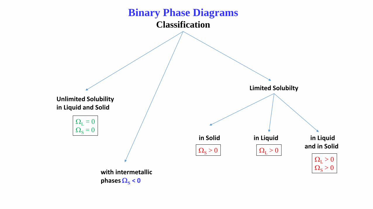
Binary Phase DiagramsClassification
WL = 0
WS = 0
Unlimited Solubilityin Liquid and Solid
Limited Solubilty
in Solid in Liquid in Liquidand in Solid
WS > 0 WL > 0
WL > 0
WS > 0with intermetallicphases WS < 0

Binary Phase Diagrams
Limited solubility in the Liquid State (WL > 0)
Regular solution
ln(gAL) = WL(1 – XA
L)2 > 0 gAL > 1
ln(gBL) = WL(1 – XB
L)2 > 0 gBL > 1 Tendency for phase separation in the liquid state
If WL> 0 a miscibility gap will form in the liquid state!

Binary Phase Diagrams
Limited solubility in the Liquid State (WL > 0)
DeHoff (2006)
WL = 0 WL = 10000 J/mol WL = 20000 J/mol

Binary Phase Diagrams
Limited solubility in the Liquid State (WL > 0)
# very different melting points
# inflection point in the liquidus curve
# retrograde solubility of Tl in Ag above 300 oC;
# very low solubility of Ag in Tl;
# Allotropic phase transition in Tl at 234 oC;
a(Tl) hexagonal P 63/mmc
ß(Tl) cubic Im-3m

Binary Phase Diagrams
Limited solubility in the Liquid State (WL > 0)
# Maximum of the liquid missibility gap at 1071 K
# WL = 2R TgmL ~ 17800 J/mol
# Eutectic point TE ~ 591 K
# below 591 K two phase mixture Pb + Zn
Zn hexagonal; Pb cubic
L1 + L2
L
L1 + Zn
Pb + Zn
TgmL
E

Binary Phase Diagrams
Limited solubility in the Liquid State (WL > 0)
●
●
●
●
●
●
A
B
C
D
F
G
A T > 1071 K homogeneous liquid L with XZn = 0.4
B L starts to segregate
XZn(L1) ~ 0.4, XZn(L2) ~ 0.92
fraction(L1) ~ 100%
C Two liquids mixture
XZn(L1) ~ 0.11, XZn(L2) ~ 0.98 (almost pure Zn melt)
fraction (L1) ~ 56 %
D The Zn-rich liquid disappears (Zn crystallizes)
Mixture of Pb-rich liquid (L1) + Zn
XZn(L1) ~ 0.06, XZn(Zn) ~ 0.999
fraction(Zn) = 38%
F Eutectic Tie-line; L1 + Pb + Zn in equilibrium
XZn(Pb) ~ 0.024, XZn(Zn) ~ 0.99
G Two phase mixture of solid Pb and solid Zn

Binary Phase Diagrams
Limited solubility in the Liquid State (WL > 0)
# Temperature of the maximum of theSolubility gap Tgm
L ~ 879 K at XPb ~0.38
# WL = 2RTgmL ~ 14600 J/mol
# B Two – liquid mixture
XPb(L1) ~ 0.13, XPb(L2) ~ 0.76
# Monotectic point M
(MM‘ – monotectic tie-line)
XPb(L1) ~ 0.016, XPb(L2) ~ 0.97 XPb(fcc) ~ 0.998
# Monotectic reaction
L2 ↔ L1 + Pb
# Below 302 K two phase mixture of Ga and Pb
Ga orthorhombic oC8 Cmca
Pb cubic cF4 F m-3m
TgmL
L1L1 + L2
L2
L
L1 + Pb
Ga + Pb
MM‘
●
B

Binary Phase Diagrams
Limited solubility in the Liquid State (WL > 0)
M
# TgmL ~ 3162 K
WL ~ 52490 J/mol
# Monotectic point M
Monotectic T = 2124 K;
# Solubility of Ag in bcc V
increases with increasing T
# Solubility of V in Ag –
negligible:
V bcc structure I m-3 m
(5+, 4+, 3+, 2+)
Ag fcc structure F m -3 m
TgmL

Binary Phase Diagrams
Limited solubility in the Liquid State (WL > 0)
# Maximum of the liquid immisibility
gap unknown →
WL probably very high
# Very high Monotectic point 3240 oC
# practically no mutual solubility
below 2000 oC

Binary Phase Diagrams
Monotetctic Reaction - DG curves

Binary Phase Diagrams
Monotectic Reactions
# temperature of the maximum of
the liquid miscibility gap 849 K
at XTl = 0.32;
# WL ~ 14100 J/mol;
# Monotectic Temperature 559 K;
# Allotropic phase transition
L1 + ß → L1 + a Tl at 234 oC;
# 2 phase mixture Ga + aTl below 30 oC.

Binary Phase Diagrams
Invariant reactions - Summary
Limited Reaction Description
Solubility
Solid Eutectic l ↔ a + ß
Eutectoid g ↔ a + ß
Peritectic l + a ↔ ß
Metatectic ß ↔ l + a
Liquid Monotectic l1 ↔ l2 + a

Binary Phase Diagrams
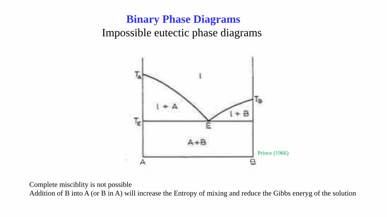
Impossible eutectic phase diagrams
Gibbs phase rule:
The invariant tie -line means that the there isno degree of freedom: the composiiton and thetemperature are fixed
Inclined tie-line in an eutectic phase diagram means thatT can be varied as a function of composition, which is notpossible.
Binary Phase Diagrams
Impossible eutectic phase diagrams
Prince (1966)
Complete misciblity is not possible
Addition of B into A (or B in A) will increase the Entropy of mixing and reduce the Gibbs eneryg of the solution

Binary Phase DiagramsClassification
WL = 0
WS = 0
Unlimited Solubilityin Liquid and Solid
Limited Solubilty
in Solid in Liquid in Liquidand in Solid
WS > 0 WL > 0
WL > 0
WS > 0with intermetallicphases WS < 0

Intermetallic Compounds
Classification
Entropy
ordered disordered
Variations in chemical composition
Stoichiometric Non-stoichiometricDefect compounds
Electronic configuration
Normal ValenceCompounds
Hume-Rotheryphases

Binary Phase DiagramsIntermediate phases - Formation
# Enthalpy stabilisation with respect to the termianl solid solutions
Strong preference for the formation of bonds between unlike atoms in the solid
De = eAB – ½ (eAA + eBB ) < 0 → WS < 0
# usually (very) different structures from the terminal solid solutions

Binary Phase DiagramsFormation of intermediate phases
WS < 0
WL = 0
# WS < 0 and WL = 0 Increase of the melting temperatures
of the solid solutions with respect to the pure components
is observed;
# congruent melting at XBCM
# Congruent melting (freezing) – the melt freezes in a solid phase
with the same composition
# Incongruent melting (freezing) – the solid and the melt do not have
the same composition
XBCM

Binary Phase DiagramsFormation of intermediate phases
Extention of the Regular solution model:
DH mix = XB(1 – XB)
WS(XB) = - a[b(1-2XB)4 + c/(d – XB)2]
The second term describes a strong tendency for
unlike bond formation
-ac/(d – XB)2 ; XB → d deep minimum
0,0 0,2 0,4 0,6 0,8 1,0
-4000
-2000
0
DH
mix
(J/m
ol)
XB
a
a+ß a+ß a
Appearance of an
intermediate phase ß
Relatively wide
compositional range
Prince (1966)
ß
WS(XB); WS(XB) < 0

Binary Phase DiagramsFormation of intermediate phases
Stoichiometric (line) compounds – compounds with
‚Infinitely‘ large curvature!!!

Binary Phase DiagramsFormation of intermediate phases
The curvature of the DG curve the ß phase determines the stability range
Prince (1966)

Binary Phase DiagramsPhase diagrams with Intermediate Phases
FeCr
s – FeCr phase
Tetragonal, P 42/mnm; 30 atoms in the unit cell
Compositional range 45 – 49 wt% Cr
Fe DHM = 13.8 kJ/mol
Cr DHM = 21.0 kJ/mol

Binary Phase DiagramsPhase diagrams with Intermediate Phases
Very large compositional range
35 – 65 wt% V!!!
Fe V
WS << 0

Binary Phase DiagramsPhase diagrams with Intermediate Phases
# Intermediate phase ß with relatively wide compositional range
# congruent melting of the ß phase for the composition X*.
# The phase diagram could be regarded as two eutectic phase
diagrams: A – X and X – B;
∂XBb/∂T ~ DHsol
ab/ T(XBß – XB
a) ∂2Gmb/∂(XB
b)2;
∂T/ ∂XBb ~ T ∂2Gm
b/∂(XBb)2 (X* – XB
a) / DHsolab ;
# very large curvature of the Gibbs free energy of the
ß phase ↔ vertical phase boundary
# very small solubility of the a phase in ß ↔
vertical phase boundary
X*
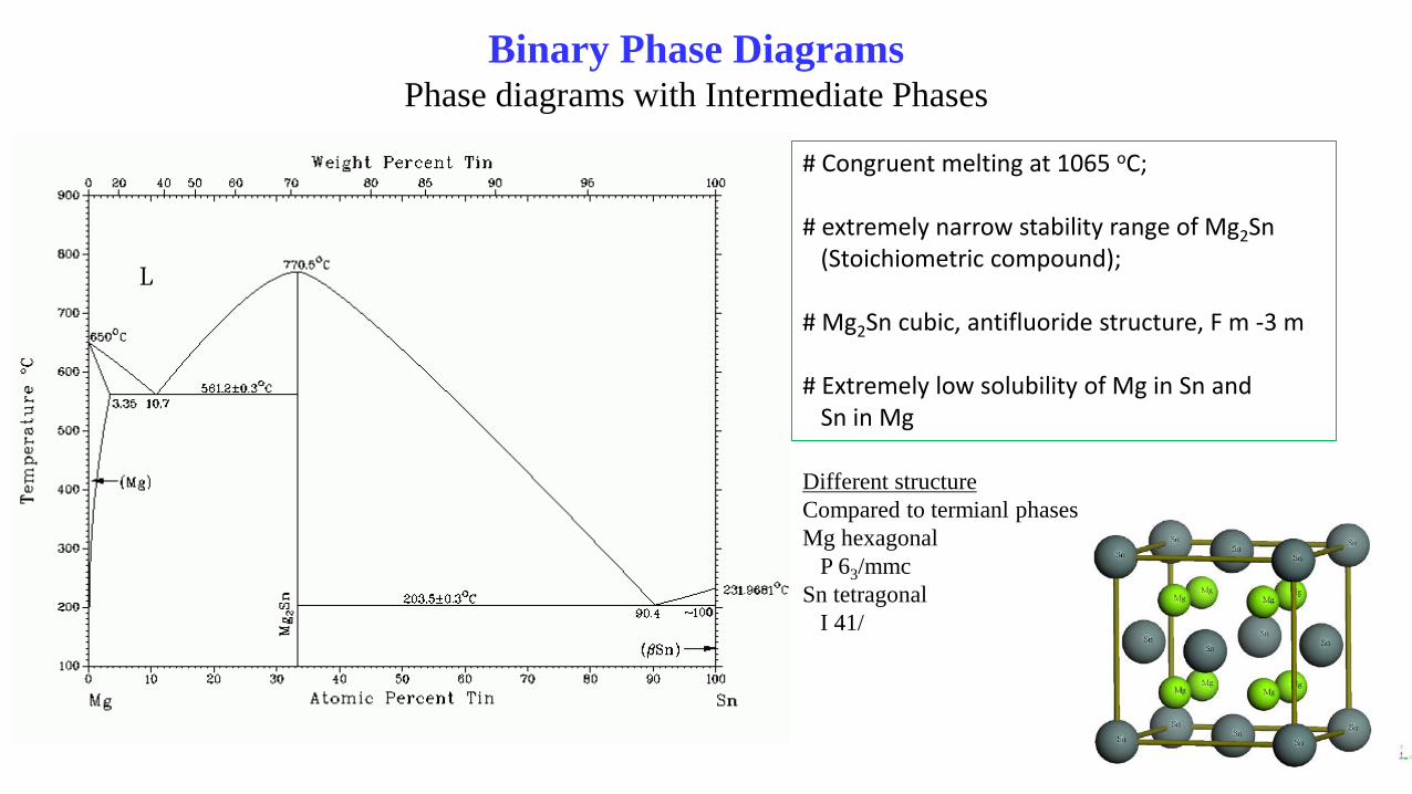
Binary Phase DiagramsPhase diagrams with Intermediate Phases
# Congruent melting at 1065 oC;
# extremely narrow stability range of Mg2Sn(Stoichiometric compound);
# Mg2Sn cubic, antifluoride structure, F m -3 m
# Extremely low solubility of Mg in Sn and Sn in Mg
Different structure
Compared to termianl phases
Mg hexagonal
P 63/mmc
Sn tetragonal
I 41/

Binary Phase DiagramsPhase diagrams with Intermediate Phases
# Congruent melting at 1065 oC
# extremely narrow stability range
(Stoichiometric compound);
# Mg2Si cubic, antifluoride structure, F m -3 m
# Extremely low solubility of Mg in Si and
Si in Mg
Mg hexagonal
P 63/mmc
Si cubic
F d -3 m

Binary Phase DiagramsPhase diagrams with Intermediate Phases
●A
●B
●
●
A Liquid with composition XSi(L) = 0.4
B L + Mg2Si
XSi(Mg2Si) = 0.333, XSi(L) = 0.45
fraction (Mg2Si) ~ 50%
C Mg2Si + Si solid state 2-phase mixture
fraction fraction (Mg2Si) ~ 89%
C

Binary Phase DiagramsPhase diagrams with Intermediate Phases
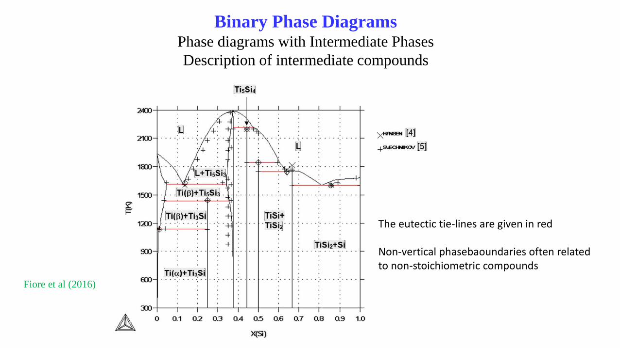
Multiple intermetallic compounds
# Ti5Si3 is congruently melting;
Larger range of stability at high temperatures
Hex P 63/mcm
# Ti3Si, Ti5Si4 and TiSi are incongruently
melting, stoichiometric compounds
# TiSi2 congruently melting
TiSi2
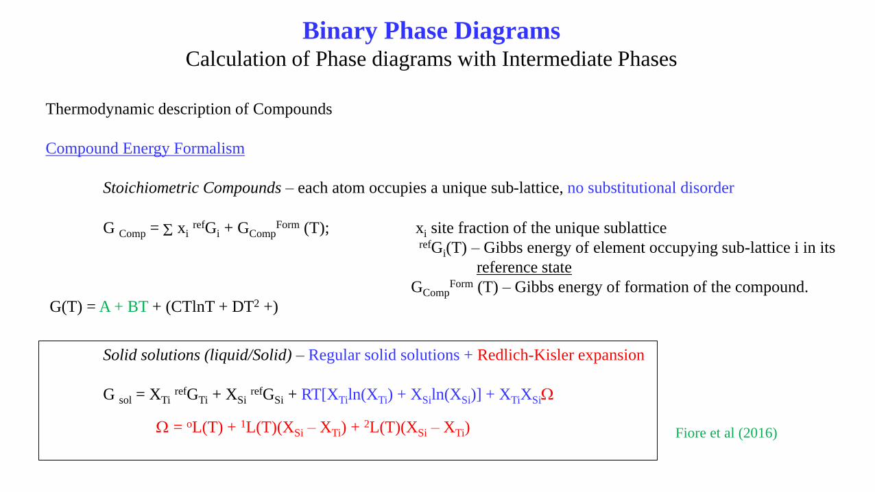
Binary Phase DiagramsCalculation of Phase diagrams with Intermediate Phases
Thermodynamic description of Compounds
Compound Energy Formalism
Stoichiometric Compounds – each atom occupies a unique sub-lattice, no substitutional disorder
G Comp = S xirefGi + GComp
Form (T); xi site fraction of the unique sublatticerefGi(T) – Gibbs energy of element occupying sub-lattice i in its
reference state
GCompForm (T) – Gibbs energy of formation of the compound.
G(T) = A + BT + (CTlnT + DT2 +)
Solid solutions (liquid/Solid) – Regular solid solutions + Redlich-Kisler expansion
G sol = XTirefGTi + XSi
refGSi + RT[XTiln(XTi) + XSiln(XSi)] + XTiXSiW
W = oL(T) + 1L(T)(XSi – XTi) + 2L(T)(XSi – XTi) Fiore et al (2016)

Binary Phase DiagramsPhase diagrams with Intermediate Phases
Description of intermediate compounds
Ti3SiSi occupies 1 sub-lattice (XSi= ¼)
Ti atoms fill 3 sub-lattices with the same sitesymmetry, each contributes XTi = ¼
Ti
Si
G Comp = S xirefGi +
Binary Phase DiagramsPhase diagrams with Intermediate Phases
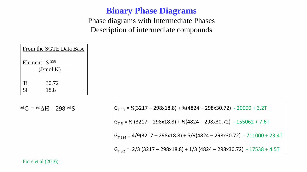
Description of intermediate compounds
From the SGTE Data Base
Element S 298
(J/mol.K)
Ti 30.72
Si 18.8
Fiore et al (2016)
GTi3Si = ¼(3217 – 298x18.8) + ¾(4824 – 298x30.72) - 20000 + 3.2T
GTiSi = ½ (3217 – 298x18.8) + ½(4824 – 298x30.72) - 155062 + 7.6T
GTi5S4 = 4/9(3217 – 298x18.8) + 5/9(4824 – 298x30.72) - 711000 + 23.4T
GTiSi2 = 2/3 (3217 – 298x18.8) + 1/3 (4824 – 298x30.72) - 17538 + 4.5T
refG = refDH – 298 refS

Binary Phase DiagramsPhase diagrams with Intermediate Phases
Description of intermediate compounds
Fiore et al (2016)
Solid solutions
Binary Phase DiagramsPhase diagrams with Intermediate Phases
Description of intermediate compounds
The eutectic tie-lines are given in red
Non-vertical phasebaoundaries often relatedto non-stoichiometric compounds
Fiore et al (2016)

Binary Phase DiagramsPhase diagrams with Intermediate Phases
CuZn
# five peritectic reactions
l + a ↔ ß
l + ß ↔ g
l + g ↔ d
l + d ↔ e
l + e ↔ h
# only the e phase is stoichiometric and
has a vertical phase boundary
# the other intermediate phases (solid
Solutions) have inclined phase boundaries,
because the curvatures of the Gibbs energy
curves are not so steep


